Modelling water temperature dynamics for eelgrass (Zostera marina) areas in the nearshore Scotian Shelf

Water temperature is an important environmental factor for many ecological processes in coastal ecosystems. Here, we study water temperature dynamics at a set of study sites on the Atlantic coast of Nova Scotia where eelgrass beds are found. The central emphasis is to predict temperature on scales relevant to coastal ecosystem processes using a high-resolution nearshore oceanographic model based on the Finite Volume Community Ocean Model (FVCOM). The model predictions were evaluated against observed temperature time series at six sites for three years from 2017-2019; the evaluation indicates that the model was able to replicate the temperature variation on time scales from hours to seasonal. We also used various biologically tailored temperature metrics relevant to eelgrass condition, including mean seasonal values and variability, daily ranges, growing degree day (GDD), and warm events, to validate the model against time series observations to better understand the temperature regime at the study sites. Frequency resolved Willmott skill scores were >0.7, and the temperature metrics were well predicted with the exception of a bias in GDD at some of the shallow sites. The eelgrass sites have a wide range of temperature conditions. Mean water temperature in the summer differed by more than 7°C between the shallowest and the deepest sites, and the rate of heat accumulation was fastest at shallow sites which had ≥ 12 extreme warm events per year. While the amplitude of the temperature variations within the high frequency band (<48 hr) was greater in shallower sites, temperature changes on meteorological time scales (48 hr to 60 days) were coherent at all sites, suggesting the importance of coast-wide processes. The results of this study demonstrated that our high resolution numerical model captured biologically relevant temperature dynamics at different time scales and over a large spatial region, and yet still accurately predicted detailed temperature dynamics at specific nearshore sites. Thus, the model can provide important insights into coastal temperature dynamics that are potentially useful for conservation planning and understanding the implications of future change.

1 Introduction

Nearshore temperature dynamics can be highly heterogeneous both spatially and temporally, due to the complex interplay of air-sea heat fluxes with localized geometry, atmospheric forcings that influence water currents and mixing, and its interaction with shelf and deep ocean physical processes. In turn, these highly variable temperature regimes have potentially significant effects on valued ecosystem components and influence coastal ecosystem processes. Eelgrass (Zostera marina) ecosystems provide important ecosystem services such as shoreline protection, water filtration, carbon storage, and fisheries maintenance (Fourqurean et al., 2012; Nordlund et al., 2016). Light, temperature, and nutrients all influence eelgrass growth and production (Lee et al., 2007; Enríquez et al., 2019). In this study, we focus on nearshore temperature dynamics which is a direct and indirect structuring elements for seagrass ecosystems, and of particular interest in the context of climate change. Previous work has shown that temperature effects on eelgrass are multi-faceted (Krumhansl et al., 2021; Wong and Dowd, 2023). Eelgrass is also susceptible to marine heatwaves that originate offshore but propagate into, and are exacerbated by, nearshore conditions (Marbà and Duarte, 2010; Moore et al., 2014; Strydom et al., 2020; Wiberg, 2023). Understanding the relationship of coastal ecosystem processes with the physical environment requires high resolution physical data across large spatial scales. Unfortunately, in the nearshore zone it is often not feasible to obtain this information from in-situ measurements or satellite data due to limitations in data resolution and spatial scales. Hence, we must rely on properly calibrated and validated numerical ocean models. Despite advances in oceanographic model developments, predicting temperature accurately and capturing its variability on the small but important spatial and temporal scales characteristic of the nearshore is difficult. The reasons include accurately representing advective processes due to complex coastlines and bathymetry, adequately resolving air-sea heat exchange and absorption, and ensuring proper dynamical coupling with the adjacent shelf. Furthermore, model predictions are most useful if they are evaluated using ecologically meaningful temperature metrics that are linked to target ecosystems or species.

Our study region is the Atlantic coast of Nova Scotia, Canada. Water temperature over the Scotian Shelf has strong spatial and seasonal variability, with the main controlling mechanism being the air-sea heat flux (sum of the flux of solar heating, sensible heat, latent heat and longwave radiation) that accounts for about 85% of the observed temperature variability (Umoh and Thompson, 1994). Cold water upwelling yields an important temperature signal in summer, and horizontal advection and vertical mixing have relatively smaller contributions. Additionally, large scale variations in water temperature over the Scotian Shelf are related to the two dominant equatorward flows over the Scotian Shelf (Thompson et al., 1988; Petrie, 2007; Brickman et al., 2018). The first is the inner-shelf current along the Atlantic coast, fed by a branch of the outflow from Gulf of St. Lawrence; and the second is the current along the shelf break, that is an extension of the Labrador Current (Sutcliffe et al., 1976). The two seasonally varying currents are topographically steered by banks, basins and channels, leading to variations in water temperature (Petrie and Drinkwater, 1993; Drinkwater, 1996; Hannah et al., 1996; Wu et al., 2016).

Numerical models of the physical oceanography in this region have emphasized the Scotian Shelf, but largely ignored the nearshore due to the difficulty in adequately resolving it, despite its importance to many valued ecosystem components such as eelgrass. During the last four decades, numerical models have been developed for the Scotian Shelf based on various types of circulation models with different model resolutions. For example, using finite element models, Han et al. (1999) and Hannah et al. (2001) investigated the seasonal variation of the circulation over the shelf with model resolution that varied from 2 km over the coastal waters to 30 km in the deep ocean. Using a nested-grid modelling system, Sheng et al. (2006) studied the response of the upper ocean to storms using a model resolution over the shelf of about 7 km. Using an ice-ocean coupled model based on the Princeton Ocean Model, Wu et al. (2012) developed a circulation model with a horizontal resolution of about 10 km, while Katavouta et al. (2016) developed an ocean circulation model based on the Nucleus for European Modeling of the Ocean (NEMO) with a horizontal resolution of 2.8 km. These models represent well the key dynamics driving large-scale temperature variations over the Scotian Shelf, but cannot accurately represent nearshore processes due to the relatively coarse model resolution used. More recently, Feng et al. (2022) developed a model based on the Finite Volume Community Ocean Model (FVCOM) for the eastern shore island area of the Scotian Shelf, however the spatial variation of water temperatures in the target eelgrass areas in this study were still not adequately resolved. The challenge to accurately modelling the nearshore temperature is the complicated bathymetry and coastlines. This requires spatial resolution down to a few meters to achieve reasonable temperature predictions, and to accurately represent the nearshore dynamics (Lynge et al., 2010; Poje et al., 2010; McWilliams, 2016).

The eelgrass areas used for this study are characterized by irregular coastlines, deep bays with steep shorelines, shallow bays with elevated intertidal flats and tidal channels, and many islands and headlands with strong tidal flows. Consequently, these eelgrass beds inhabit a wide range of environmental conditions, from shallow, warm, protected waters to deep, cool, exposed waters (Wong, 2018; Krumhansl et al., 2021). Eelgrass beds also experience high temporal variability in water temperature from not only localized processes such as air-sea heat fluxes (i.e., local forcing), but also tidal and wind driven advective heat fluxes originating on the shelf (i.e., remote forcing) (Wong et al., 2013; Wong and Dowd, 2021). To understand the dynamics of water temperature in the eelgrass areas, in this study we develop a high resolution numerical oceanographic model which uses an unstructured mesh that allows for very high spatial resolutions at sites of interest. This allows us to represent the complex coastline and bathymetry and to provide accurate water temperature predictions where needed. Using the model results, we examine ecologically meaningful temperature metrics (i.e., mean temperature, heat accumulation, daily temperature range, thermal physiological threshold exceedances) that are known to influence seagrass growth and productivity (Krumhansl et al., 2021; Wong and Dowd, 2023). Finally, a simple heat budget is developed to identify the primary mechanisms underlying the temperature dynamics at select study sites.

2 Materials and methods

2.1 Model configuration

The ocean model used in this study is the FVCOM 4.4, which is a finite-volume, unstructured grid ocean model (Chen et al., 2007, 2003). The model has a free surface, uses sigma coordinates in the vertical direction, and employs a mode time split. FVCOM solves the three-dimensional momentum, continuity, temperature and salinity equations by computing fluxes between unstructured triangular elements. The unstructured mesh system in the model is able to fit complex coastlines and enables a seamless transition between small-scale processes in eelgrass areas and large-scale processes in the adjacent shelf and open ocean, while maintaining computational efficiency. The model domain and model grid size are shown in Figure 1. The model mesh includes 176755 nodes and 335819 elements. The horizontal resolution of the model mesh varies from 1-2 km in the open shelf to 10 m in the near-shore waters. An example of where locally very high resolution is important is Port l’Hebert, where the water temperature is strongly associated with the water advection through a narrow channel with the width less than 100 m (Figure 1A).

Figure 1

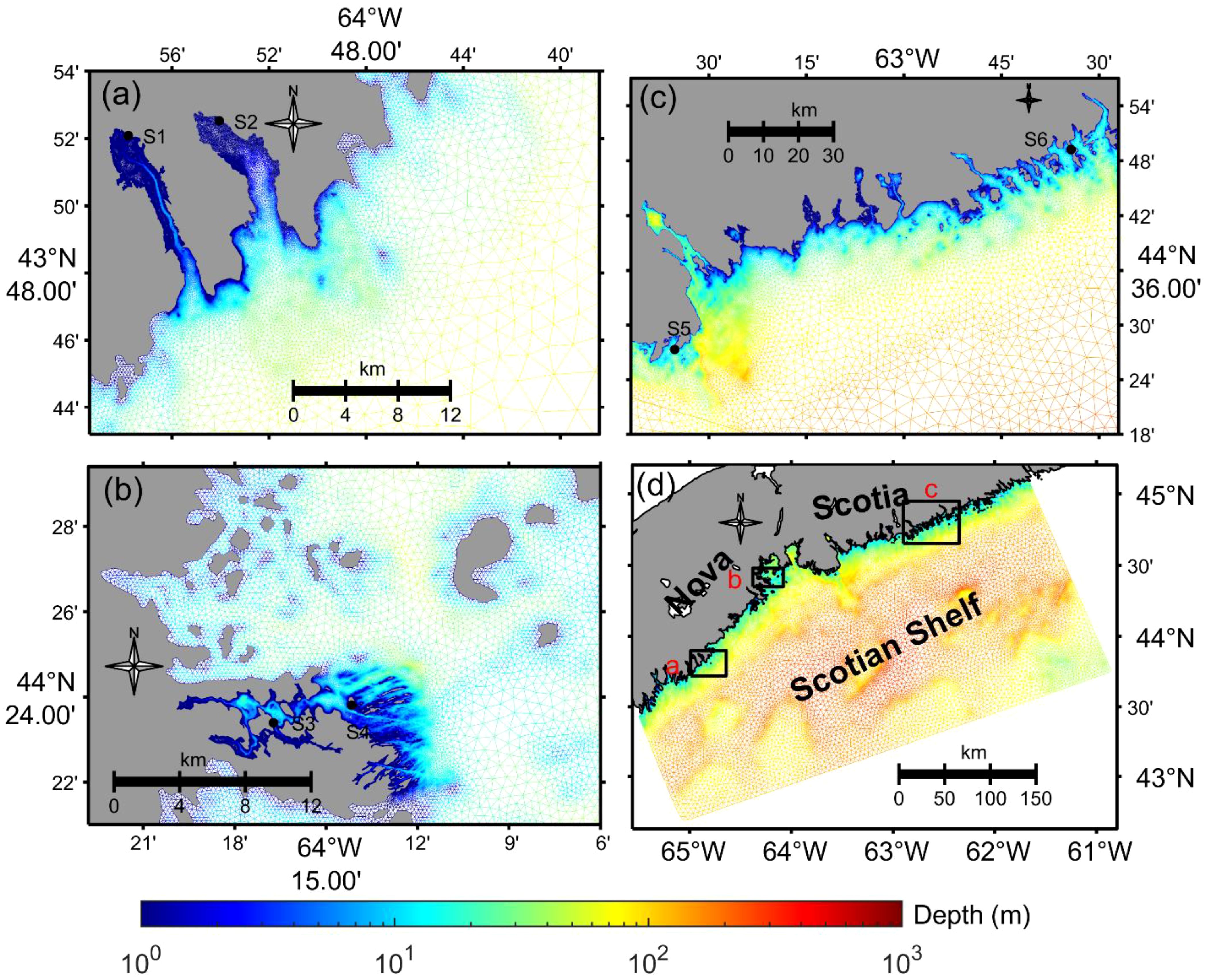
Figure 1 Map showing the model domain, depth, and the computational mesh, along with the eelgrass study sites: Model domain (D) and details of the model mesh resolutions for core study areas (A-C). The locations of all study sites are the sites listed in Table 1. The designations S1-S6 refer to Port l’Hebert, Port Joli, Mason’s Island, Sacrifice Island, Sambro, and Taylor Head, respectively.

The model bathymetry is based on high resolution survey data (10 m in our study areas) from the Canadian Hydrographic Service (CHS). The model bathymetry is further smoothed in elements where the Haney number (a measure of the horizontal pressure gradient (HPG) error, Haney, 1991) is larger than 6. The bathymetry smoothing was locally within the depth of a node and those of the neighbor nodes (5-7 nodes). The aim of the smooth is to avoid large errors caused by the HPG over steep slopes induced by the sigma levels. It is worthy to note that the bathymetry is smoothed locally, the water depth of an element with the Haney number larger than 6 is averaged with its depth and the depth of elements around it. The water column with the minimum water depth of 0.1 m is divided into 30 layers in the vertical. In this study, a generalized sigma coordinate system was used (Chen et al., 2012). For water depths shallower than 60 m, the sigma levels are uniformly distributed through the water column. For water depths deeper than 60 m, we used a generalized coordinate system to resolve the bottom boundary layer and to reduce the horizontal pressure gradient error: 10 uniform layers in the surface layer with an interval of 2 m, 5 uniform layers in the bottom layer with a 2 m interval, and 15 levels stretched to span the center of the water column. Vertical turbulent mixing is modelled with the General Ocean Turbulence Model (GOTM) using a k-ϵ formulation (Umlauf and Burchard, 2005), and the horizontal diffusion is parameterized as the Smagorinsky diffusivity with a coefficient of 0.1. The heat flux is calculated with Coupled Ocean–Atmosphere Response Experiment (COARE) 2.6 (Webster and Lukas, 1992).

The temperature and salinity of the model are initialized from the daily reanalysis results of GLORYS12v1 with 1/12° resolution (Jean-Michel et al., 2021). The open boundary conditions employ a one-way nesting scheme with variables (water elevations, temperature, salinity and currents) from GLORYS12v1. The tidal components are also included through the nesting; the tidal water elevations and tidal currents of eight major tidal constituents (M2, S2, N2, K2, O1, K1, P1, and Q1) are from the tidal dataset of TPXO9 (Egbert et al., 1994; Egbert and Erofeeva, 2002). Surface atmospheric forcing consists of wind at 10 m above the ocean surface, air temperature at 2 m, relative humidity at 2 m, precipitation, evaporation, shortwave radiation, and longwave radiation. We obtained these forcings with 1/4° resolution from ERA5 reanalysis datasets from the European Centre for Medium-Range Weather Forecasts. The FVCOM model as configured above outputted hourly 3D total currents, temperature, and sea level for the period of 2016 – 2022.

2.2 In-situ observations for model validation

Bottom water temperature and water pressure (i.e., sea level) were recorded at six eelgrass sites along the Atlantic coast of Nova Scotia, Canada (Figure 1, Table 1). These sites represent a range of environmental conditions over which eelgrass beds occur, including gradients of temperature, light, sediment properties, and water movement, all influenced by tidal currents, winds, waves, and bathymetry (Bakirman and Gumusay, 2020; Krumhansl et al., 2020, 2021; Wong and Dowd, 2021). Port l’Hebert, Port Joli, and Mason’s Island are the shallower sites (mean depth at high tide< 2 m) with muddy/silty sediments, low current speed, and low exposure to waves and offshore processes (Table 1, Figure 1). Other beds (Sacrifice Island, Taylor Head, and Sambro) were located in deeper water (mean depth at high tide > 3 m), with sandy sediments, higher current speeds, and higher exposure to waves and offshore dynamics (Table 1, Figure 1) (Krumhansl et al., 2020; Wong and Dowd, 2021).

Table 1

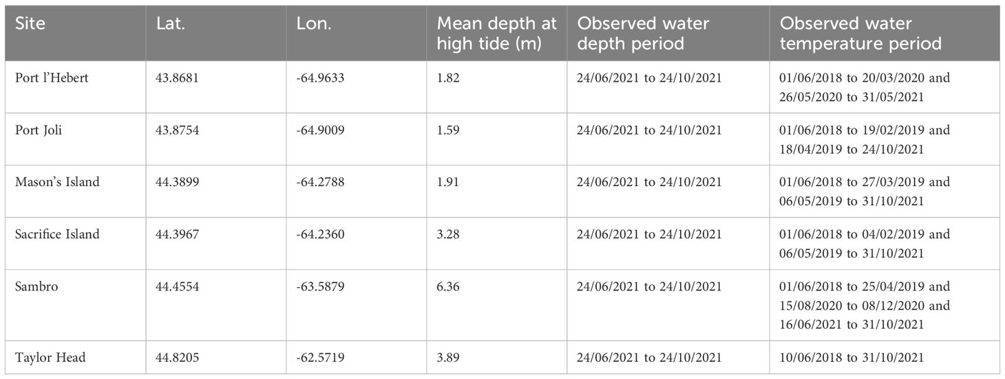
Table 1 Location, mean depth, and the period of observations at the six eelgrass sites.

Water depth was calculated from water pressure measurements made at 10 cm above the bed at 10 minutes intervals using HOBO pressure sensors (Onset Corp) during 24 July 2020 to 24 November 2021, and used for observing sea level variation. We used the water temperature records by HOBO tidbit temperature loggers (Onset Corp) at 10 cm above the bed and logged data every 15 minutes from 1 June 2018 to 31 October 2021, and used these data for model validation. The observed data were generally recorded continuously although some logistical challenges resulted in shorter deployments at some sites (Table 1). All the loggers were placed directly in the eelgrass beds to record the actual conditions that the eelgrass experiences. At some shallow sites, this meant that loggers were periodically exposed to the air at very low tides, as were the seagrass beds. Temperature recordings from exposure were thus sometimes higher (>30 °C) and lower (below freezing) than expected if the loggers had remained submerged. Extreme air temperatures have been shown to impact seagrasses (Park et al., 2016), so we elected to retain these temperatures.

2.3 Data analysis

2.3.1 Validation of water level

The tidal components of sea level from FVCOM are compared to those from sea level records at the eelgrass sites for five selected dominant principal tidal constituents (O1, K1, N2, M2, and S2 with periods of 25.84 hr, 23.92 hr, 12.66 hr, 12.42 hr, 12.00 hr, respectively), four overtides (M4, S4, M6, and M8 with periods of 6.21 hr, 6.00 hr, 4.14 hr, 3.11 hr, respectively), and one compound tide (2MK5 with period of 4.93 hr) with a signal-to-noise ratio greater than 2. The amplitudes and phases of the tidal constituents are calculated using the T-Tide toolbox of Pawlowicz et al. (2002).

2.3.2 Prediction of temperature variations

The temperature time series from both the observations and model predictions were processed to isolate signals in different frequency bands, specifically: (i) low frequency (changes occurring over with periods > 60 days); (ii) middle frequency (changes that occur with periods ranging from 48 hr to 60 days); and (iii) high frequency (temperature changes that occur with periods ≤ 48 hr). This corresponds to the time series decomposition

$\begin{array}{ll}T(t)=T_{seas}(t)+T_{met}(t)+T_{tidal}(t)& (1)\end{array}$

where t is time, T(t) is the original temperature series, T_seas (t) is the low frequency seasonal cycle, T_met (t) is the mid frequency meteorological band variations, and T_tidal (t) includes the high frequency with tidal and daily periods. Note that spectral gaps typically exist between these bands. Low frequency temperature changes, T_seas (t), are related to seasonal and annual cycles (on the order of months to years). Middle frequency temperature variations, T_met (t), are associated with meteorological events such as storms and wind driven upwelling events that advect cold deeper water onshore and rapidly drop the temperature (Platt, 1971), or any processes with time scales of days to weeks. High frequency temperature changes, T_tidal (t), are usually related to tidal exchanges and daily heating and cooling processes (period of 10 - 48 hr). Overtides also contribute to high frequency temperature variation, and are usually harmonics of the principal tidal constituents with periods of 3-10 hr. The analysis was carried out as follows. T_seas (t) was determined by fitting polynomial functions to the raw temperature data at each site that captured the seasonal cycle. To fit the seasonal cycle (Equation 1) we chose a polynomial rather than sinusoids since the typical shape of the seasonal cycle was non-sinusoidal and readily captured with a low order polynomial. Otherwise, it would have required the superposition of a number of sinusoids and different frequencies (plus an offset or trend) in order to capture the shape properly. The de-seasonalized time series, or anomalies, were then calculated by subtracting the fitted seasonal cycle, T_seas (t), from the original temperature time series, T (t). This yields the temperature anomaly T_met (t) + T_tidal (t). A low-pass filter was then applied to the temperature anomaly time series to obtain the meteorological (mid frequency) band, T_met (t). The high frequency (tidal/daily) band, T_tidal (t), was then calculated by subtracting the T_met (t) from the temperature anomaly.

Time series of the three different frequency bands at each site were compared for the observations and model predictions using the Willmott skill (WS, Willmott, 1981), defined as:

$\begin{array}{ll}WS=1-MSE/\langle {(\left|m-\langle o\rangle \right|+\left|o-\langle o\rangle \right|)}^2\rangle & (2)\end{array}$

where $MSE=\langle {(m-o)}^2\rangle$ is the mean square error, m and o are time series of the modelled and observed variables, respectively, and $\langle \rangle$ represents a mean. The highest (1) and lowest (0) values of WS show perfect agreement and complete disagreement between the model predictions and observations, respectively. This method has been used previously for assessment of numerical models for simulation of different parameters in aquatic environments (e.g., Warner et al., 2005; Wilkin, 2006; Liu et al., 2009). In addition to this frequency resolved WS, summary statistics of the bottom water temperature including mean, maximum, and minimum temperatures, standard deviation (SD), and the 95^th percentile are used to compare the model predictions and observations.

2.3.3 Spectral analysis of water temperature

A power spectral analysis of the bottom water temperature at each site for both the observed data and model predictions was performed. These analyses help with identifying the dominant frequencies of the water temperature variation (e.g., diurnal tides, solar heating and cooling, semi-diurnal tides, overtides and compound tides in shallow waters), as well as assessing the capability of the model in computing them as compared to those found in the observations.

2.3.4 Eelgrass specific temperature metrics

Model accuracy in prediction of water temperature metrics ecologically relevant for eelgrass were also evaluated and include: growing degree days (GDD); warm water events that exceed physiological thresholds; and daily temperature range.

The thermal integral, known as growing degree days (GDD), has been used in horticulture and fish studies to predict growth and development (Neuheimer and Taggart, 2007). GDD quantifies heat accumulation over time in a system and has been shown to influence eelgrass productivity and resilience (Krumhansl et al., 2021; Wong and Dowd, 2023). Here, GDD from model predictions and from in-situ observations is estimated by:

$\begin{array}{ll}GDD(t)={\displaystyle {\int }_{t_0}^{t}max((T_{max}+T_{min})/2-T_{base},0)}dt& (3)\end{array}$

Where, when a full year of observed data available at all sites, $T_{max}$ and $T_{min}$ are the daily maximum and minimum temperature, respectively, and $T_{base}$ is a prescribed base temperature. GDD is calculated for 01 June 2018 ($t_0$) to 25 April 2019 where almost a full year of observed data are available at all sites. Eelgrass photosynthesis increases rapidly from 0 to 5°C, while a maximum in the ratio of photosynthesis to respiration (P:R) occurs at 5°C (Biebl et al., 1971; Marsh et al., 1986). Therefore, we elected to use 5°C as $T_{base}$ in our calculations of GDD, as done previously in Krumhansl et al. (2021).

We also calculated the frequency and duration of warm water events that exceeded known physiological thermal thresholds for eelgrass using both the model predictions and the observed data. We used three different temperature thresholds (T_th) of 20°C, 23°C, and 27°C. The 23°C temperature is typically considered the physiological threshold for temperate eelgrass above which respiration begins to outpace photosynthesis, causing reduced or even negative P:R ratios that result in reduced eelgrass growth and survival (Lee et al., 2007). However, eelgrass is highly adaptable, and plants in warm conditions likely have higher temperature thresholds while plants in cooler conditions have lower ones. We thus also used 20°C and 27°C as thresholds. Individual warm water events were identified as those occurring above the temperature thresholds for ≥ 2 hr, with distinct events separated by ≥ 3 days, akin to the definition for marine heatwaves (Oliver et al., 2018; Krumhansl et al., 2021).

Finally, to estimate the daily temperature range, the difference between the daily 90^th and 10^th percentiles are calculated and compared between the model predictions and observed data. The probability density of the daily temperature ranges are also calculated using kernel density estimation.

2.3.5 Nearshore heat balance

A simple heat budget is applied to the FVCOM model results to estimate the relative contributions of different processes that can contribute to the warming or cooling of the water in the immediate region around 2 selected eelgrass sites with different physical dynamics. Here the heat budget is applied following standard approaches for the coastal regions (Dever and Lentz, 1994; Lemagie et al., 2021, 2020). The heat budget in a generic form may be expressed as

$\begin{array}{ll}\frac{\partial \overline{T}}{\partial t}=\frac{Q}{\rho C_{p}H}+\frac{1}{H}{\displaystyle {\int }_{-H}^0\stackrel{\rightharpoonup }{u}·\nabla Tdz+\epsilon }& (4)\end{array}$

where $\overline{T}$ is the mean temperature in the box surrounding the site extended to the shoreline (i.e., depth and laterally averaged water temperature, Supplementary Figure S7), $Q$ is the surface heat flux, $\rho$= 1024.6 kg m^-3 is the reference density of seawater, $C_P$ = 4002.5 J kg^-1° C^-1 is its heat capacity, H is the depth, and $\stackrel{\rightharpoonup }{u}$ is the horizontal velocity. The left-hand side of Equation 4 shows the rate of temporal change in the heat content, or temperature tendency, of the region ($\delta T^{Avg}$). The first term on the right-hand side is the heat flux through the surface ($\delta T^{SHF}$), and the second term estimates the advective heat flux ($\delta T^{Adv}$). Finally, the last term is the residual of the balance ($\epsilon$), which could be due to processes such as mixings, eddies, or other complex three-dimensional processes that were not captured by this simple heat budget. To evaluate the contribution of each term on the temperature change over the region, each term in Equation 4 is expressed as an equivalent temperature change in units of °C hr^-1. The heat budget is also integrated over time to assess the variation of each term for different seasons. When a triangular cell is treated as dry, the water temperature (salinity) is calculated as a wet triangular cell except the flux through the boundaries of this triangle is zero. Freshwater inputs are quite small for all the study sites and are not included in the model.

3 Results

3.1 Sea level

Figure 2 shows the amplitude and phase of sea level for selected tidal constituents at Port l’Hebert and Taylor Head (selected as representative shallow and deep sites, respectively, with the remaining sites presented in Supplementary Figure S1). Of all the principal tidal constituents, the M2 tide has the largest amplitude (> 0.55 m) across all the sites. Shallower sites [Port l’Hebert (Figure 2B), Port Joli (Supplementary Figure S1B), and Mason’s Island (Supplementary Figure S1D)] are generally associated with higher amplitude of harmonic constituents than the deeper sites [Taylor Head (Figure 2D), Sacrifice Island (Supplementary Figure S1J), and Sambro (Supplementary Figure S1L)]. While there are differences between the modelled and observed phase for principal tidal constituents (< 30°) (Figures 2E-H; Supplementary Figure S1E-H, S1M-P), the errors in prediction of amplitude and phases of the principal and harmonic tidal constituents are generally within the error standard deviation associated with their calculations (Figures 2; Supplementary Figure S1).

Figure 2

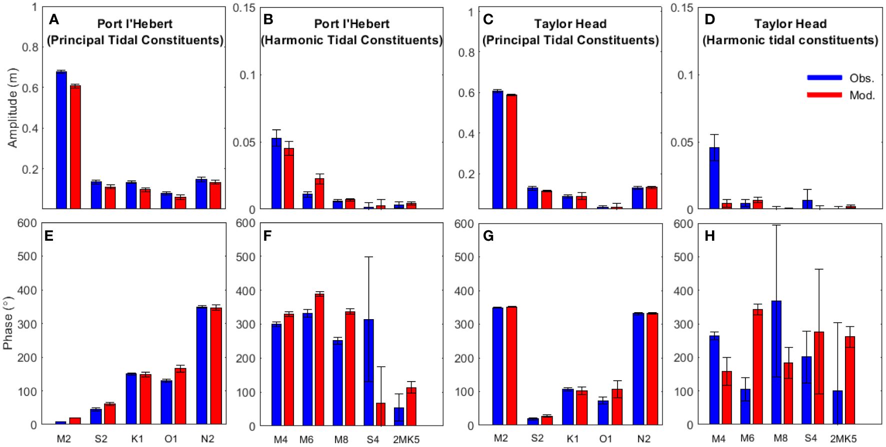
Figure 2 Amplitude (top) and phase (bottom) of sea level for five select principal tidal constituents (M2, S2, K1, O1, and N2; panels A, E, C, G) and five harmonic tidal components (M4, M6, M8, S4, and 2MK5; panels B, F, D, H) from observed data (blue) and model results (red) for 2 select sites: Port l’Hebert, a shallow site (panels A, B, E, F) and Taylor Head, a deep site (panels C, D, G, H). Length of the error bars show the standard deviation.

3.2 Water temperature variations

Comparison of the bottom water temperature from the model and observations (Figures 3, 4; Supplementary Figures S2-S5) shows that the model can predict the time series of the observed data, as well as the temperature variations at different frequencies, with Willmott skill greater than 0.7 (Table 2). In comparisons of the low frequency time series, the model consistently overestimates summer water temperatures at Port l’Hebert [max 7.2°C for the observed data (Figure 3A) and 1.7-2.5°C for the of low frequency data (Figure 3B)] and Port Joli [max 4.4°C for the observed data (Supplementary Figure S2A) and 0.5-3.1°C for the low frequency data (Supplementary Figure S2B)], the two shallow sites. Note that some discrepancies for the observed data at these sites are influenced by temperature spikes associated with the sensors being exposed briefly to air (as noted above). In contrast, the model underestimated summer water temperature at the deeper sites (Figures 4A, B; Supplementary Figures S3A, B, S4A, B, S5A, B) with the maximum discrepancy of 6.6°C at Sacrifice Island (Supplementary Figures S4A, B). The model predictions of time series of the middle and high frequency temperature variations were generally within 2°C of those observed (Figures 3C, D, 4C, D; Supplementary Figures S3C, D, S4C, D, S5C, D), with the maximum discrepancies of 4.7°C at Sambro (Supplementary Figures S5C, D).

Figure 3

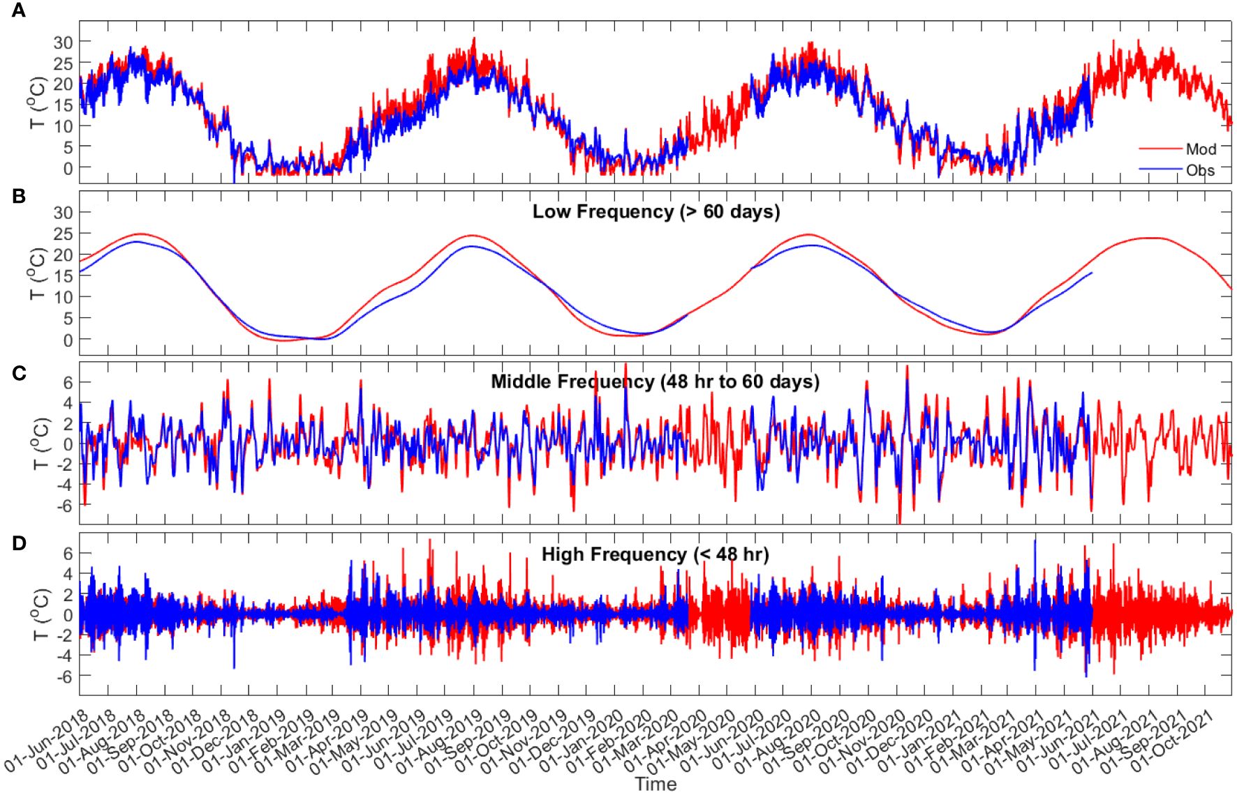
Figure 3 Port l’Hebert bottom water temperature time series (A), and time series of the bottom water temperature in low (> 60 days (seasonal band); (B), middle (48 hr to 60 days (meteorological band); (C), and high [< 48 hr; (D)] frequencies from observation data (blue) and model results (red).

Figure 4

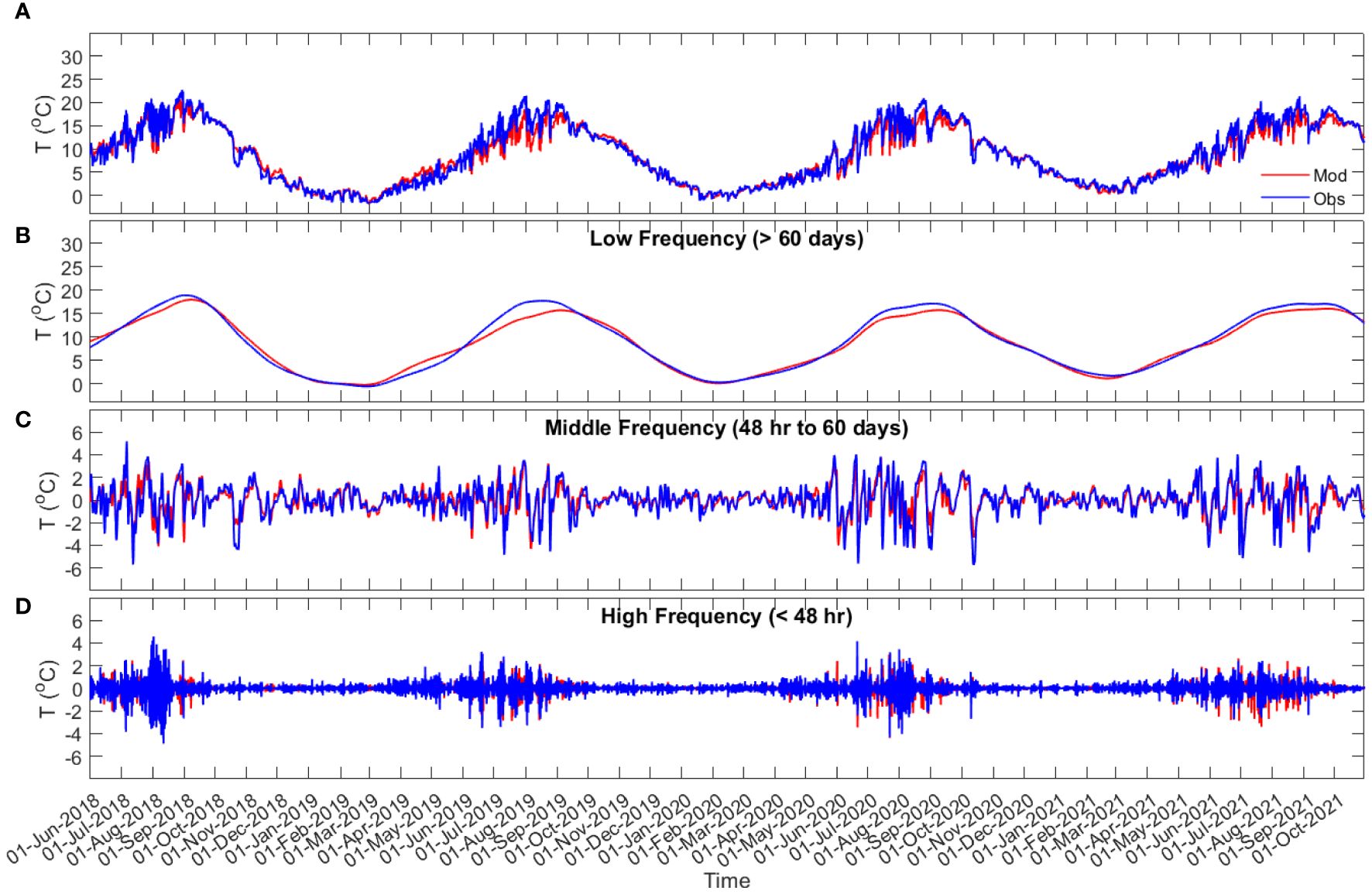
Figure 4 Taylor Head bottom water temperature time series (A), and time series of the bottom water temperature in low (> 60 days (seasonal band); (B), middle (48 hr to 60 days (meteorological band); (C), and high [< 48 hr; (D)] frequencies from observation data (blue) and model results (red).

Table 2

Table 2 Average Willmott skill score for the bottom water temperature prediction decomposed by frequency.

Across all sites, the bottom water temperature showed a seasonal trend of increasing water temperature during the spring with a maximum in August, and declining throughout the fall to a winter minimum in February (Figures 3, 4; Supplementary Figures S2-S5). The largest seasonal ranges (> 32°C) were at Port l’Hebert and Port Joli with an observed summer maximum of 28.81°C and 29.57°C, respectively, and a winter minimum of -3.97°C and -3.89°C, respectively (Table 3), again being influenced by air exposure of the recorders. The lowest seasonal range (22.14°C) was observed at Sambro (Supplementary Figures S5A, B). Temperature changes within the meteorological band at Port l’Hebert (Figure 3C) and Port Joli (Supplementary Figure S2C) were similar and did not show large inter-seasonal variations. The highest amplitude within the meteorological band (peaks usually > 1°C; SD > 1.7°C) was also calculated in these two sites relative to others, with minimum amplitudes (generally< 2°C; SD< 1°C) in Mason’s Island (Supplementary Figure S3C) and Sacrifice Island (Supplementary Figure S4C). Large consistent drops (~6°C) in the meteorological band at Sambro (Supplementary Figure S5C) could be attributed to the high winds in fall.

Table 3

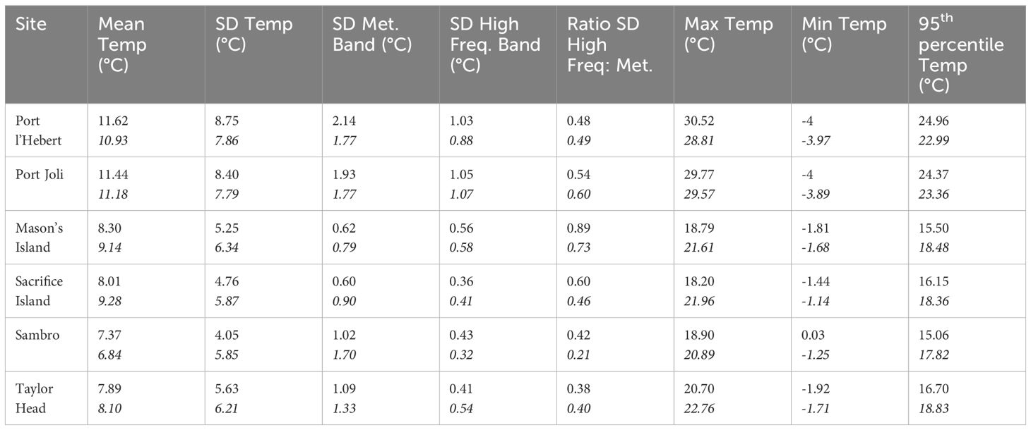
Table 3 Summary statistics of the bottom water temperature for the period 01/06/2018 to 31/05/2021 from model results and observation data (bottom row for each site in italics) at each site including mean, maximum, and minimum temperatures, temperature variability (standard deviation (SD)), and the 95^th percentile temperature.

As with the variations found in the meteorological band, the highest amplitudes of the temperature variations within the high frequency band were at Port l’Hebert (Figure 3D) and Port Joli (Supplementary Figure S2D). Of the deeper sites, Mason’s Island (Supplementary Figure S3D) and Sacrifice Island (Supplementary Figure S4D) show the highest and lowest amplitudes of variations, respectively. Inter-seasonal changes within the high frequency band were evident in all the sites with the highest amplitudes during June to September, which could be an indicator of increased heating and cooling related to solar heating and tides during warmer periods, or due to the establishment of localized horizontal temperature gradients. The highest (8.0°C) and the lowest (2.3°C) values of the summer peaks in the high frequency band were in Port Joli and Sacrifice Island, respectively. The highest (1.05°C) and the lowest (0.36°C) SD in the high frequency band from the model results were also obtained in Port Joli and Sacrifice Island, respectively (Table 3). The ratios of the standard deviation of the high frequency to meteorological band was less than 1 in all the sites from both the model results and observations (Table 3), which shows that the processes within the meteorological band can dominate the temperature dynamics at these eelgrass sites.

The model calculation of the summary statistics (time series during 01/06/2018 to 31/05/2021) of the bottom water temperature are within 2°C of the observed data in most sites (Table 3). The warmest mean bottom water temperature was in Port l’Hebert and Port Joli (11.62°C and 11.44°C, respectively) and the coldest mean temperature was in Sambro and Taylor Head (7.37°C and 7.89°C, respectively) from the model calculations. The highest maximum temperature, the highest 95^th percentile temperature, and the lowest minimum temperatures calculated from both the model and observed data were found at Port l’Hebert and Port Joli. These sites also have the highest standard deviation of the temperature, which is an indicator of having the highest temperature variations among all the sites.

3.3 Spectral analysis

Spectral analysis of the bottom water temperature shows that the model can reproduce the dominant water temperature variations found in each observed time series from the eelgrass sites (Figure 5). Dominant frequencies are associated with the meteorological band (>48 hr) followed by diurnal variations, which also includes diurnal tides as well as temperature variation from solar heating, and finally semi-diurnal tides (~12 h). The presence of these frequencies at all sites in the power spectra of bottom water temperature indicates the strong effect of these processes on temperature dynamics. From the power spectra, the influence of solar and tidal heating at the shallower sites (i.e., Port l’Hebert (Figure 5A), Port Joli (Figure 5B), and Mason’s Island (Figure 5C) with mean depth at high tide< 2 m; Table 1) was greater than the other sites (i.e., Sacrifice Island (Figure 5D), Sambro (Figure 5E), and Taylor Head (Figure 5F), mean depth at high tide >3m; Table 1). Peaks at frequencies associated with overtides (periods of 3-10 hr) were evident at most sites (we note the model underestimation in most sites). The most significant overtides occurred at Port l’Hebert, Port Joli, and Mason’s Island due to the relatively strong bottom friction, while overtides were less evident in the temperature spectrum of Sacrifice Island, and were negligible in Taylor Head and Sambro, the deepest sites.

Figure 5

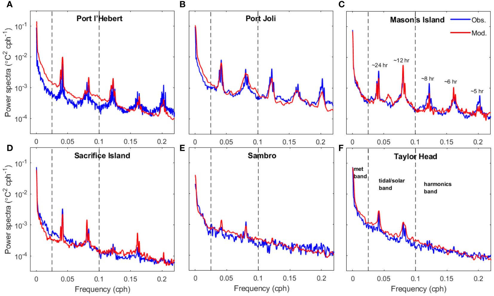
Figure 5 Power spectra of bottom water temperature from observed data (blue) and model results (red) at Port l’Hebert (A), Port Joli (B), Mason’s Island (C), Sacrifice Island (D), Sambro (E), and Taylor Head (F). Dashed lines show the limits of the low, middle, and high frequency bands considered (see panel F). The periods associated with the peaks in frequencies are shown in panel C.

3.4 Eelgrass specific temperature metrics

3.4.1 Summary statistics for the growing season

To highlight the differences among sites for eelgrass growth, summary statistics in the summer growing period were calculated. These metrics were averaged over summer periods (June 1-Sept 15) between 01/06/2018 and 31/05/2021) (Table 4). From the model calculations, the warmest temperatures were at Port l’Hebert and Port Joli (22.14°C and 21.57°C, respectively) and the coldest temperatures at Sambro (9.19°C), while intermediate temperatures were found at Mason’s Island, Sacrifice Island, and Taylor Head (13.64°C, 12.43°C, and 12.70°C, respectively). Model calculations and observed data also show the highest maximum temperature and 95^th percentile temperature at Port l’Hebert and Port Joli, but the lowest minimum temperature in Sambro and Taylor Head. Generally, the model calculation of the summary statistics during the summer growing period are within 2°C of the observed data (Table 4).

Table 4

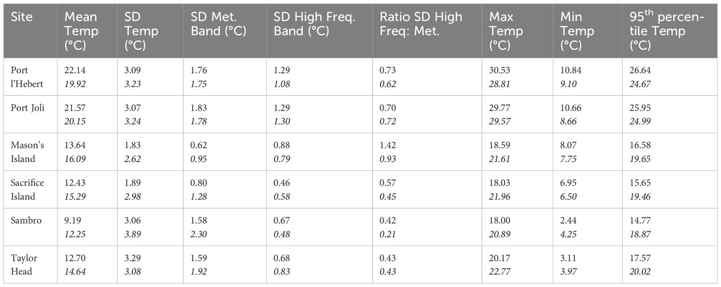
Table 4 Summary statistics of the bottom water temperature from model results and observation data (bottom row for each site in italics) during the summer growing periods (time series of summer periods of June 1-Sept 15 between 01/06/2018 and 31/05/2021) at each site including mean, maximum, and minimum temperatures, temperature variability [standard deviation (SD)], and the 95^th percentile temperature.

3.4.2 Growing degree day

Figure 6 shows plots GDD during 01 June 2018 to 25 April 2019 at all sites (Table 1). The discrepancies between the GDD from the model predictions and those from the observations are< 19% and strongly influenced by the bias in the mean temperature between model and observations in the bottom water time series (Figures 4A, 5A; Supplementary Figures S2A-S5A). The largest discrepancies were observed for Mason’s Island and Sacrifice Island. Heat accumulation varies across the sites, with heat accumulating earliest and fastest at Port l’Hebert and Port Joli, at intermediate levels for Mason’s Island, Sacrifice Island, and Taylor Head, and being latest and slowest at Sambro. Maximum heat accumulation was highest at Port l’Hebert and Port Joli, and lowest at Sambro. Heat accumulation was associated with depth, with heat accumulation reaching highest maximums and having highest rates of accumulation (i.e., initial slope in GDD) at shallow sites (Port l’Hebert, Port Joli) as compared to deeper sites. Accumulation of heat happened in the spring, summer, and fall from both model and observed data with negligible accumulation in winter, starting in December, when the temperature dropped below the set threshold of 5°C used in the GDD calculation (Equation 3) (Figure 6).

Figure 6

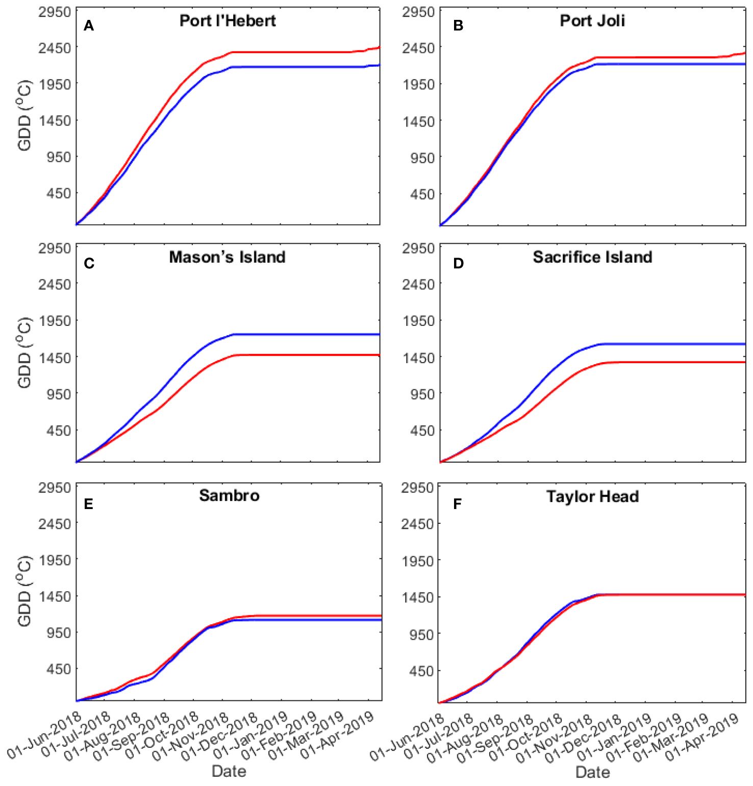
Figure 6 Growing degree days at Port l’Hebert (A), Port Joli (B), Mason’s Island (C), Sacrifice Island (D), Sambro (E), and Taylor Head (F) from the model (red) and observations (blue) for the growing season period 01/06/2018 to 25/04/2019.

3.4.3 Warm water events

Warm water events, where the bottom water temperature is > 20°C, 23°C, or 27°C for > 2 hr and each event is separated by > 3 days, is calculated from 10/06/2018 to 31/05/2021 (Figure 7). This period covers three summer seasons with the observed data available from all sites except for summer 2019 in Sambro, where the warm events are less likely due to the large depth (Krumhansl et al., 2020; Wong and Dowd, 2021). From the observations and the model results, the warm water events only occurred at Port Joli and Port l’Hebert based on both the 23°C and 27°C criteria (Figures 7B, C, E, F), while other sites also experience warm events based on 20°C criteria (Figures 7A, D). Based on 23°C, an average of 15.3 events year^-1 in Port Joli (from observations and model), and 16.3 and 11.3 events year^-1 from model and observations, respectively, in Port l’Hebert (Figure 7B) were evident. These events occurred during June to September (Figure 4A; Supplementary Figure S2A) with an average duration of 12.7 and 6.78 hr per event from model and observations, respectively, in Port Joli and 16.9 and 10.7 hr per event from model and observations, respectively, in Port l’Hebert. It is notable that the calculated numbers of warm events were highly dependent on the definition of these events (e.g., duration, length, and separation of events) due to high temporal variations of temperature. That is, a small change in the definition could result in quite different values, e.g. based on a 27°C threshold from the model results, an average of 3 events year^-1 with an average duration of 3.7 hr occurred in Port Joli, and an average of 5.3 events year^-1 with an average duration of 5.5 hr occurred in Port l’Hebert. The duration and number of events based on 20°C criteria were much higher than those based on 23°C and 27°C. Specifically, short durations of warm events (≤ 3 hr) based on 20°C are observed in the sites that are deeper than Port l’Hebert and Port Joli (the model did not predict warm events in Mason’s Island, Sacrifice Island, and Sambro). The discrepancies in the mean duration of events between the model results and those from the observed data were generally within the standard deviation of calculations (Figures 7D–F).

Figure 7

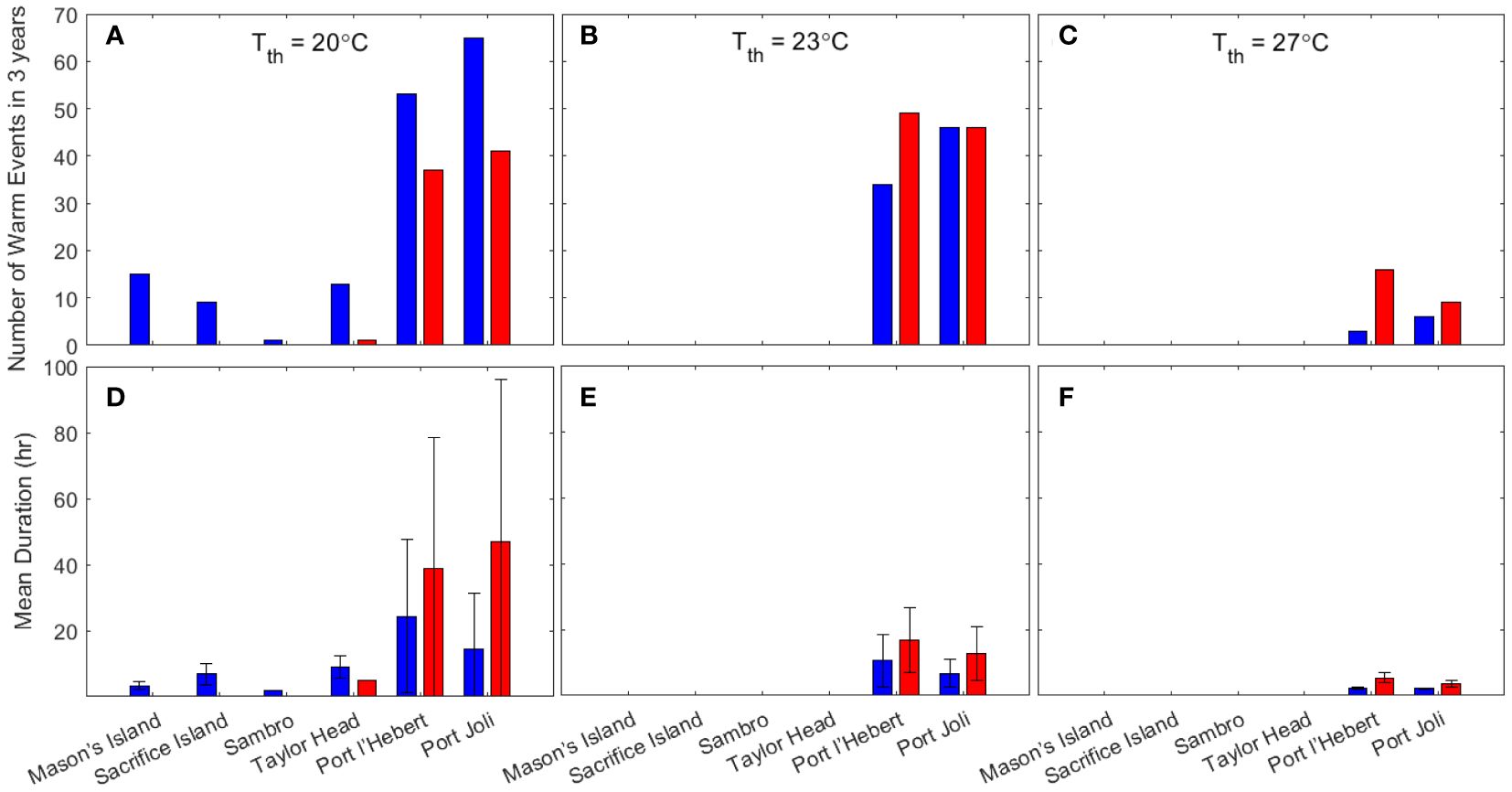
Figure 7 Number (A–C) and duration (D–F) of warm events (for ≥ 2 hr; distinct events are separated by ≥ 3 days) when the bottom water temperature is greater than the threshold temperature (T_th) of 20°C (A, D), 23°C (B, E) and 27°C (C, F) for the growing seasonal period 10/06/2018 to 31/05/2021 from the model (red) and observations (blue). The length of the error bars in D-F correspond to the standard deviations.

3.4.4 Daily temperature variabilities

Figure 8 compares the daily bottom water temperature range and its probability density estimate (via kernel density estimation) for the eelgrass sites. Shallow sites in general experienced higher daily temperature variations with lower peak probability and greater spread than the deeper sites, e.g., maximum monthly average of daily range in Port l’Hebert (Figure 8A) and Port Joli (Figure 8C) was 5°C, compared to< 3°C in Sambro (Figure 8I) and Taylor Head (Figure 8K). A daily temperature range of > 10°C also occurred occasionally in Port l’Hebert and Port Joli. While the daily variations show a seasonal trend across all sites, with increased values during the warm seasons (June-September), shallower sites can experience daily variations > 5°C during the winter seasons. Daily temperature variations can be due to daily solar heating and cooling and tidal advection (Krumhansl et al., 2020), as well as occasional wind driven changes that can amplify water temperature changes.

Figure 8

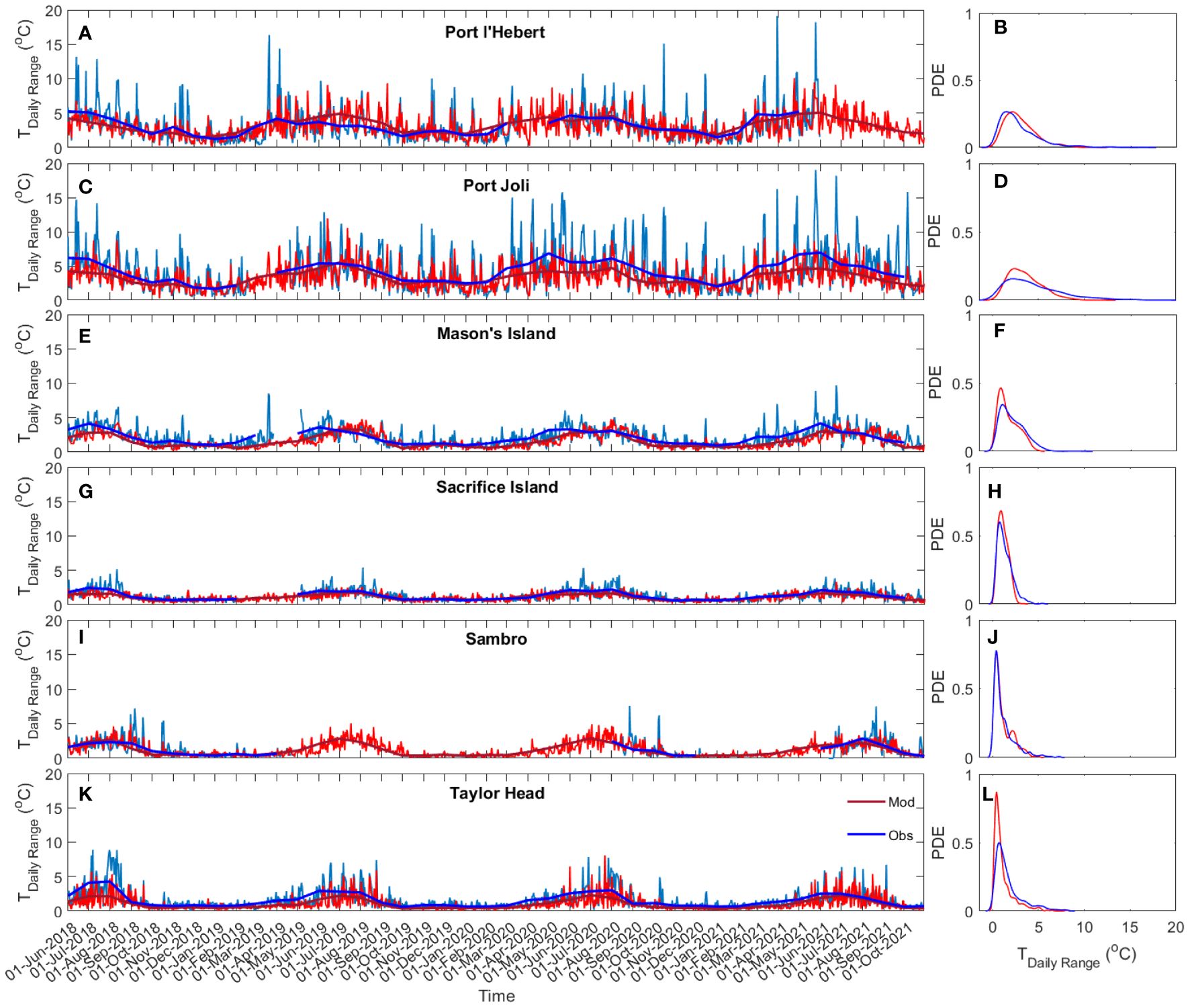
Figure 8 Time series (A, C, E, G, I, K) and probability density estimate (PDE; B, D, F, H, J, L) of daily bottom water temperature range at Port l’Hebert (A, B), Port Joli (C, D), Mason’s Island (E, F), Sacrifice Island (G, H), Sambro (I, J), and Taylor Head (K, L) from observed data (light and dark blue showing daily and monthly average, respectively) and model results (light and dark red: daily and monthly average, respectively).

3.5 Heat balance

The heat balance during the three years from 2019 to 2021 was calculated using model results at Port l’Hebert and Taylor Head to illustrate the seasonal contribution of different factors to temperature changes at these two sites that contrast in both depth and exposure (daily-averaged values shown in Figure 9 and note the scale difference in the y-axes between the two sites). While a seasonal variability is evident in the change in the heat content at both sites ($\delta T^{Avg}$; Figures 9A, C), with the maximum values during the warm seasons (~June-September), $\delta T^{Avg}$ values at Port l’Hebert are greater than those at Taylor Head. Specifically, $\delta T^{Avg}$ at Taylor Head is negligible during colder seasons (~November-February) with maximum daily-averaged values less than 0.03°C hr^-1. These observed variabilities in temperature change are consequence of the contributing factors to the overall heat content at each site (Equation 4).

Figure 9

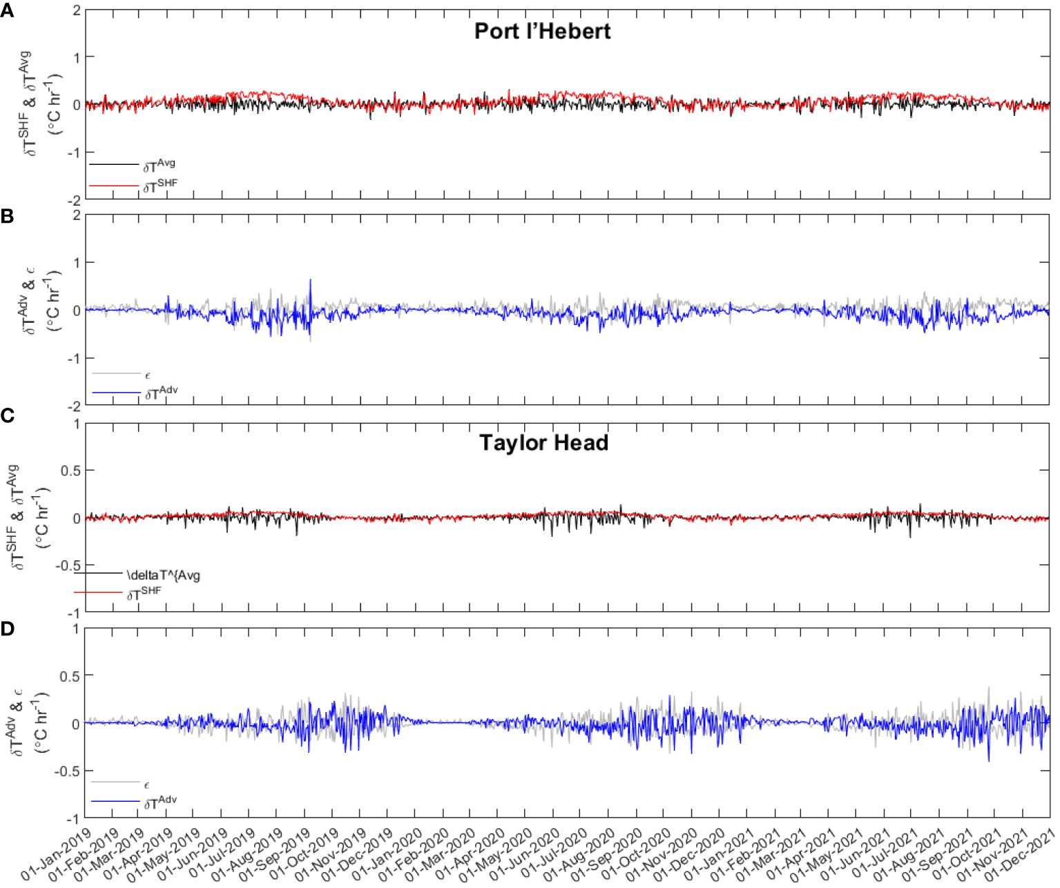
Figure 9 Daily averaged temporal change in the heat content ($\delta T^{Avg}$; black), surface heat flux ($\delta T^{SHF}$; red), advective flux ($\delta T^{Adv}$; blue), and heat budget balance residual ($ϵ$; grey) at Port l’Hebert (A, B) and Taylor Head (C, D). Note the scale difference in the y-axes between the two sites.

Heat flux through the surface ($\delta T^{SHF}$) shows a seasonal variability with higher values during the warm seasons (Figures 9A, C) at both sites. Higher $\delta T^{SHF}$ at Port l’Hebert compared to Taylor Head (e.g., maximum summer daily-averaged values of > 0.25°C hr^-1 vs< 0.1°C hr^-1, respectively) could be due to the difference in the depth of the sites as the surface heat flux per unit area at these two sites are comparable (Supplementary Figure S6). Low values of $\delta T^{SHF}$ in the winter at Taylor Head (maximum daily-averaged values< 0.05°C hr^-1) indicates negligible contribution of surface heat flux in the cold seasons at this site. The advective flux at both sites ($\delta T^{Adv}$) (Figures 9B, D) show also seasonal variations with peak values during warm seasons.

Figure 10 shows the monthly mean of each term in the heat budget at both sites computed from daily-averaged values for 3 years (2019-2021). The monthly temperature change ($\delta T^{Avg}$) was small, for any year, at the sites. In all years, the mean temperature change in the warmer months (<0.02°C hr^-1) was 1-2 orders of magnitude smaller than the contribution to the temperature change from the mean surface heat flux (0.2°C hr^-1 and 0.05°C hr^-1, at Port l’Hebert and Taylor Head, respectively). Monthly mean contribution from advective fluxes in the warm months appeared to anti-correlate with the incoming surface heat flux showing that these processes largely compensate for each other at the study sites.

Figure 10

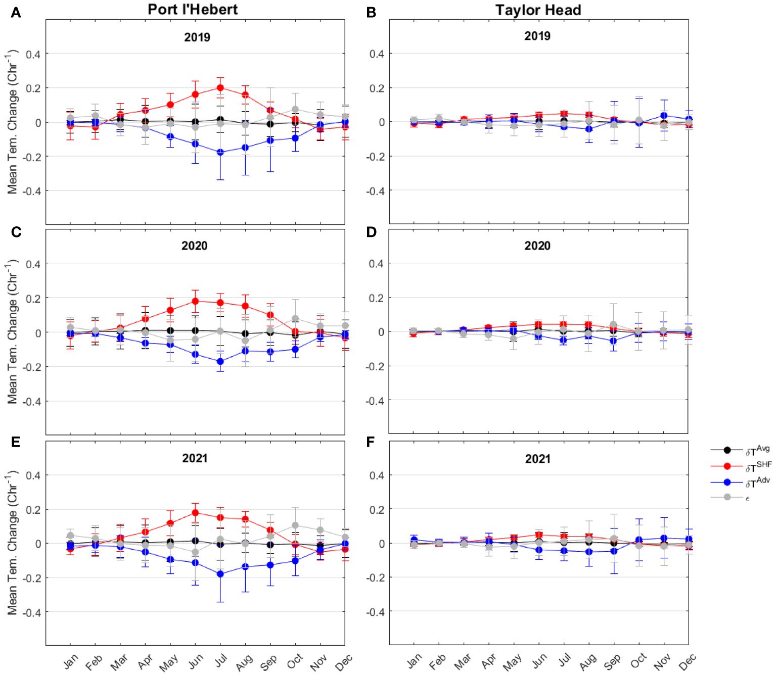
Figure 10 Monthly mean of each term in heat budget (change in the heat content of the cross section ($\delta T^{Avg}$; black), surface heat flux ($\delta T^{SHF}$; red), advective flux ($\delta T^{Adv}$; blue), and heat budget balance residual ($ϵ$; grey) at Port l’Hebert (A, C, E) and Taylor Head (B, D, F) in 2019 (A, B), 2020 (C, D), and 2021 (E, F). The length of the error bars show the standard deviation.

Monthly mean magnitude of each term in the heat budget show similar values during the 3 years of the calculation, which suggests little interannual variability at both sites (Figure 10). The monthly contribution of the residuals in the heat budget (Figures 9C, D) was generally less than the leading term at both sites throughout the 3 years (Figure 10). The residuals could be due to factors not represented well in the simple formulation used in this study (e.g., eddies or other complex 3D processes; Equation 4).

4 Discussion and conclusions

We investigated temperature dynamics in nearshore regions of the Atlantic coast of Nova Scotia on time and space scales relevant for coastal ecosystem processes. Time series of water temperature from observations and FVCOM numerical model results for June 2018 to May 2021 at six different eelgrass sites were used for validation and characterization of temperature regime. We demonstrated that the numerical model can generally predict well the key attributes of temperature relevant to eelgrass ecosystems, and do so across large spatial scales, in this case the whole Atlantic coast of Nova Scotia. We therefore argue that validating models against observations using biologically ‘fit for purpose’ temperature metrics is important to ensure that relevant attributes are well predicted, such as thermal exceedances, heat accumulation, heat wave events and daily temperature variation. Moreover, a properly calibrated and validated numerical model allows for detailed site-specific characterization of the temperature regime, as was demonstrated for the various study site. It can also help identify at-risk areas for target ecosystems resulting from temperature stress, now and in the future (Krumhansl et al., 2020; Wong and Dowd, 2021).

An overall good agreement between the numerical model predictions and the observed temperature was found. The model simulated time series of the water temperature had a Willmott skill > 0.7, and we were able to assess this in a frequency dependent manner, a feature which extends the Willmott skill score concept (Equation 2). Summary statistics during the summer growing period from the model were within 2°C of the recorded data in most sites (Table 4). The discrepancies between growing degree day from the model calculation and the observations (≤ 19%) were consistent with the systematic differences in the time series of water temperature. While the number and duration of warm events highly depended on the definition used (e.g., duration, length, and separation of events) due to the high temporal variation of temperature, the discrepancies in the mean duration of events between the model results and those from the observed data were generally within the error standard deviation of calculations.

The main discrepancies between the model and the observations were in the summer temperatures at the shallow sites (Port l’Hebert and Port Joli), which were consistently overestimated. It is important to identify such biases and consider their implications when using numerical models predictions to assess ecological implications of various temperature processes (e.g., growing degree days is quite sensitive to this discrepancy). Potential reasons are the following. Firstly, model bathymetries in the tidal channels may be too shallow, which would significantly limit exchange processes, in particular a decrease in the inward advection of cold offshore water and overestimated water temperature in the inner bay. Also, any local smoothing of bathymetry would lower the resolution of channels which ventilate the shallow intertidal flats and hence affect the temperature dynamics there. Secondly, the horizontal resolution of the air forcing (e.g., air-sea heat fluxes) from ERA5 is 31 km, which is relatively coarse compared to the model resolution used in this study. Hence, some coastal bays (e.g., Port l’Hebert and Port Joli) are represented as being on land in ERA5, which may cause artificially high water temperatures in summer (note the coarse ERA5 resolution can lead to underestimation of water temperature in deeper exposed sites by not underrepresenting the land). Thirdly, the overestimated water temperature in summer could also be caused by the uncertainty in solar radiation attenuation properties in the bottom layer, where the solar radiation not only heats the water, but also the bottom sediment due to the shallow water depth. Since the amount of the solar energy stored in the sediment is unknown, we considered all the solar energy as being distributed through the water column. To examine this process, we ran the model with different water column attenuation coefficients for solar radiation and found that the model performance can be improved by tuning them, however, development of a realistic attenuation parameterization in the bottom layer is beyond the scope of the present paper.

Previous studies have suggested that short-term, sub-seasonal temperature processes (i.e., warming events, wind events, upwelling) can play an important role in eelgrass growth and productivity (Wong et al., 2013, 2020, 2021; Krumhansl et al., 2021). However, it is important to note that the ecological function of seagrass beds is also influenced by the underwater light environment and its variations (Enríquez et al., 2019), which can act separately and together with temperature effects. The characterization of the temperature regime for our study sites indicated a similar seasonal variation in the bottom water temperature, but variability on sub-seasonal scales was markedly different across the sites. Higher water temperature in the high frequency band (<48 hr; Table 3; Figures 4D, 5D; Supplementary Figures S2D-S5D), larger dominance of solar heating and diurnal tides relative to the semi-diurnal tides (Figure 2), and relatively higher daily temperature range (Figures 8; Supplementary Figure S6) indicate a greater impact of processes on time scales< 48 hr at shallow sites (Port l’Hebert, Port Joli, Mason’s Island) compared to the other sites. Temperature variations in the meteorological band that were observed in all the sites (Figures 4C-5C; Supplementary Figures S2C-S5C) can be due to local wind events as well as coast-wide processes such as storms and wind-driven coastal upwellings. A coastal upwelling index based on Ekman transport and upwelling favorable winds (Petrie et al., 1987) has shown strong coherence with the meteorological temperature band in eelgrass sites at the eastern Scotian Shelf (Krumhansl et al., 2021), which can transfer cool nutrient rich water to the surface and support eelgrass growth and photosynthesis during periods of nutrient limitation (Sandoval-Gil et al., 2019).

Extended high temperature can have negative impacts on eelgrass health. Physiological impacts on eelgrass occur within 1-7 days when temperatures are 19-28°C (Evans et al., 1986; Gao et al., 2017), or as short as 15 min at > 30°C. Our results showed > 2 hr warm water events occurred only at Port Joli and Port l’Hebert based on 23°C (optimum temperature for photosynthesis; > 12 events year^-1) and 27°C thresholds, while other sites experienced these events based on a 20°C criteria. In shallow sites, these events are likely due to long periods of solar heating over the extensive shallow flats (Wong et al., 2013). Warm water events based on the 23°C threshold typically lasted > 10 hr. The high frequency of warm events in the eelgrass sites in this study suggest that these eelgrass frequently experienced physiologically unfavorable conditions. Alternatively, anomalous warming can result in persistent changes in eelgrass bed characteristics across multiple clonal generations and years (DuBois et al., 2020). Previous studies show that these events are typical on the Atlantic coast of Nova Scotia (Wong et al., 2013; Wong, 2018; Krumhansl et al., 2021), and that eelgrass can thermally adapt to varying temperature regimes, similar to other seagrass species (Marin-Guirao et al., 2016).

The simple heat balance analysis contrasting a shallow protected bay (Port l’Hebert) and a deeper exposed (Taylor Head) site showed that while the maximum annual changes in the heat content at the shallow site are greater than those at the deep site, the surface heat flux is the main contributor to the temperature variations during summer growing seasons at both sites (Figure 10). Monthly mean contribution of the advective fluxes in both sites was negative and buffering the surface heating in the warm months. Higher values of surface heat flux (related to daily heating and cooling) and advective flux (related to tidal exchanges), which are of the high frequency temperature changes, during warm months can be an indicator of higher amplitudes of temperature variations within the high frequency during these periods. Monthly mean magnitude of the contributing terms in the heat budget showed small interannual variabilities at both sites. Heat budgets are an important way to determine to what degree a study site is dominated by local processes versus being driven by offshore ocean dynamics, with potential implications for understanding ecosystem functioning. They are readily computed from numerical model output, but difficult to obtain directly from temperature observations.

In summary, the FVCOM model developed for this study was able to reasonably predict water temperature variations and thermal metrics relevant to eelgrass condition. The representation of nearshore dynamics and its impact on coastal water temperature across large spatial scales can only be achieved by using targeted calibrated and validated high resolution numerical models. Furthermore, we argue that the validation process for these models should be targeted to the ecosystem process of interest, using specific variables (e.g. temperature) and biologically tailored metrics. In this way, we can improve our general understanding of the interaction between the physical and biological processes in the coastal environments, as well as by taking into account other key physical drivers such as light. It is hoped that results of this study, and the numerical model developed here, can contribute towards the understanding, conservation and protection of coastal ecosystems, and the maintenance of their functioning and resilience in this era of climate change.

Data availability statement

The original contributions presented in the study are included in the article/Supplementary Material. Further inquiries can be directed to the corresponding author.

Author contributions

AJ: Conceptualization, Data curation, Formal Analysis, Methodology, Software, Validation, Visualization, Writing – original draft, Writing – review & editing, Supervision. YW: Conceptualization, Data curation, Funding acquisition, Investigation, Methodology, Project administration, Resources, Software, Supervision, Writing – original draft, Writing – review & editing. MW: Conceptualization, Data curation, Funding acquisition, Investigation, Methodology, Project administration, Resources, Supervision, Writing – original draft, Writing – review & editing. MD: Conceptualization, Formal Analysis, Methodology, Supervision, Writing – original draft, Writing – review & editing.

Funding

The author(s) declare financial support was received for the research, authorship, and/or publication of this article. MD was supported by an NSERC Discovery grant.

Acknowledgments

We thank L Zhai, RHorwitz, and YMa at the Bedford Institute of Oceanography for insightful reviews.

Conflict of interest

The authors declare that the research was conducted in the absence of any commercial or financial relationships that could be construed as a potential conflict of interest.

Publisher’s note

All claims expressed in this article are solely those of the authors and do not necessarily represent those of their affiliated organizations, or those of the publisher, the editors and the reviewers. Any product that may be evaluated in this article, or claim that may be made by its manufacturer, is not guaranteed or endorsed by the publisher.

Supplementary material

The Supplementary Material for this article can be found online at: https://www.frontiersin.org/articles/10.3389/fmars.2024.1374884/full#supplementary-material

References

Bakirman T., Gumusay M. U. (2020). A novel GIS-MCDA-based spatial habitat suitability model for Posidonia oceanica in the Mediterranean. Environ. Monit. Assess. 192. doi: 10.1007/s10661-020-8198-1

PubMed Abstract | CrossRef Full Text | Google Scholar

Biebl R., McRoy C. P., Marsh J. A., Dennison W. C., Alberte R. S. (1971). Effects of temperature on photosynthesis and respiration in eelgrass (Zostera marina L.). J. Exp. Mar. Bio. Ecol. 101, 257–267. doi: 10.1016/0022-0981(86)90267-4

CrossRef Full Text | Google Scholar

Brickman D., Hebert D., Wang Z. (2018). Mechanism for the recent ocean warming events on the Scotian Shelf of eastern Canada. Continental Shelf Res. 156, 11–22. doi: 10.1016/j.csr.2018.01.001

CrossRef Full Text | Google Scholar

Chen C., Beardsley R. C., Cowles G., Qi J., Lai Z., Gao G., et al. (2012). An unstructured-grid, finite-volume community ocean model: FVCOM user manual (Cambridge, MA, USA: Sea Grant College Program, Massachusetts Institute of Technology).

Google Scholar

Chen C., Huang H., Beardsley R. C., Liu H., Xu Q., Cowles G. (2007). A finite volume numerical approach for coastal ocean circulation studies: Comparisons with finite difference models. J. Geophys. Res. Ocean 112. doi: 10.1029/2006JC003485

CrossRef Full Text | Google Scholar

Chen C., Liu H., Beardsley R. C. (2003). An unstructured grid, finite-volume, three-dimensional, primitive equations ocean model: application to coastal ocean and estuaries. J. Atmos. Ocean. Technol. 20, 159–186. doi: 10.1175/1520-0426(2003)020<0159:AUGFVT>2.0.CO;2

CrossRef Full Text | Google Scholar

Dever E. P., Lentz S. J. (1994). Heat and salt balances over the northern California shelf in winter and spring. J. Geophys. Res. Ocean. 99, 16001–16017. doi: 10.1029/94JC01228

CrossRef Full Text | Google Scholar

Drinkwater K. F. (1996). Atmospheric and oceanic variability in the Northwest Atlantic during the 1980s and early 1990s. J. Northwest Atlantic Fishery Sci. 18. doi: 10.2960/J.v18.a6

CrossRef Full Text | Google Scholar

DuBois K., Williams S. L., Stachowicz J. J. (2020). Previous exposure mediates the response of eelgrass to future warming via clonal transgenerational plasticity. Ecology 101, 1–12. doi: 10.1002/ecy.3169

CrossRef Full Text | Google Scholar

Egbert G. D., Bennett A. F., Foreman M. G. G. (1994). TOPEX/POSEIDON tides estimated using a global inverse model. J. Geophys. Res. Ocean. 99, 24821–24852. doi: 10.1029/94JC01894

CrossRef Full Text | Google Scholar

Egbert G. D., Erofeeva S. Y. (2002). Efficient inverse modeling of barotropic ocean tides. J. Atmos. Ocean. Technol. 19, 183–204. doi: 10.1175/1520-0426(2002)019<0183:EIMOBO>2.0.CO;2

CrossRef Full Text | Google Scholar

Enríquez S., Olivé I., Cayabyab N., Hedley J. D. (2019). Structural complexity governs seagrass acclimatization to depth with relevant consequences for meadow production, macrophyte diversity and habitat carbon storage capacity. Sci. Rep. 9, 14657. doi: 10.1038/s41598-019-51248-z

PubMed Abstract | CrossRef Full Text | Google Scholar

Evans A. S., Webb K. L., Penhale P. A. (1986). Photosynthetic temperature acclimation in two coexisting seagrasses, Zostera marina L. and Ruppia maritima. Aquatic Botany. 24, 185–197. doi: 10.1016/0304-3770(86)90095-1

CrossRef Full Text | Google Scholar

Feng T., Stanley R. R. E., Wu Y., Kenchington E., Xu J., Horne E. (2022). A high-resolution 3-D circulation model in a complex archipelago on the coastal scotian shelf. J. Geophys. Res. Ocean. 127, 1–23. doi: 10.1029/2021JC017791

CrossRef Full Text | Google Scholar

Fourqurean J. W., Duarte C. M., Kennedy H., Marbà N., Holmer M., Mateo M. A., et al. (2012). Seagrass ecosystems as a globally significant carbon stock. Nature Geoscience. 5 (7), 505–509. doi: 10.1038/ngeo1477

CrossRef Full Text | Google Scholar

Gao Y., Fang J., Du M., Fang J., Jiang W., Jiang Z. (2017). Response of the eelgrass (Zostera marina) to the combined effects of high temperatures and the herbicide, atrazine. Aquatic Botany. 142, 41–47. doi: 10.1016/j.aquabot.2017.06.005

CrossRef Full Text | Google Scholar

Haney R. L. (1991). On the pressure gradient force over steep topography in sigma coordinate ocean models. J. Phys. Oceanogr. 21, 610–619. doi: 10.1175/1520-0485(1991)021<0610:OTPGFO>2.0.CO;2

CrossRef Full Text | Google Scholar

Hannah C. G., Loder J. W., Wright D. G. (1996). “Seasonal variation of the baroclinic circulation in the Scotia-Maine region,” in Buoyancy Effects on Coastal and Estuarine Dynamics. Eds. Aubrey D. G., Friedrichs C. T. (American Geophysical Union), 7–29. doi: 10.1029/CE053p0007

CrossRef Full Text | Google Scholar

Hannah C. G., Shore J. A., Loder J. W. (2001). Seasonal circulation on the Western and Central Scotian shelf. J. Phys. Oceanogr. 31, 591–615. doi: 10.1175/1520-0485(2001)031<0591:SCOTWA>2.0.CO;2

CrossRef Full Text | Google Scholar

Jean-Michel L., Eric G., Romain B.-B., Gilles G., Angélique M., Marie D., et al. (2021). The copernicus global 1/12° Oceanic and sea ice GLORYS12 reanalysis. Front. Earth Sci. 9. doi: 10.3389/feart.2021.698876

CrossRef Full Text | Google Scholar

Katavouta A., Thompson K. R., Lu Y., Loder J. W. (2016). Interaction between the tidal and seasonal variability of the Gulf of Maine and Scotian shelf region. J. Phys. Oceanogr. 46, 3279–3298. doi: 10.1175/JPO-D-15-0091.1

CrossRef Full Text | Google Scholar

Krumhansl K. A., Dowd M., Wong M. C. (2020). A characterization of the physical environment at eelgrass (Zostera marina) sites along the Atlantic coast of Nova Scotia. Can. Tech Rep. Fish Aquat Sci., 213 p.

Google Scholar

Krumhansl K. A., Dowd M., Wong M. C. (2021). Multiple metrics of temperature, light, and water motion drive gradients in eelgrass productivity and resilience. Front. Mar. Sci. 8. doi: 10.3389/fmars.2021.597707

CrossRef Full Text | Google Scholar

Lee K.-S., Park S. R., Kim Y. K. (2007). Effects of irradiance, temperature, and nutrients on growth dynamics of seagrasses: A review. J. Exp. Mar. Bio. Ecol. 350, 144–175. doi: 10.1016/j.jembe.2007.06.016

CrossRef Full Text | Google Scholar

Lemagie E., Kirincich A., Lentz S. (2020). The summer heat balance of the Oregon inner shelf over two decades: mean and interannual variability. J. Geophys. Res. Ocean. 125, 1–18. doi: 10.1029/2019JC015856

CrossRef Full Text | Google Scholar

Lemagie E., Kirincich A., Lentz S. (2021). The summer heat balance of the Oregon inner shelf over two decades: mean and interannual variability. J. Geophys. Res. Ocean. 126, 1–18. doi: 10.1029/2020JC016720

CrossRef Full Text | Google Scholar

Liu Y., MacCready P., Hickey B. M., Dever E. P., Kosro P. M., Banas N. S. (2009). Evaluation of a coastal ocean circulation model for the Columbia river plume in summer 2004. J. Geophys. Res. Ocean. 114, 1–23. doi: 10.1029/2008JC004929

CrossRef Full Text | Google Scholar

Lynge B. K., Berntsen J., Gjevik B. (2010). Numerical studies of dispersion due to tidal flow through Moskstraumen, northern Norway. Ocean Dyn. 60, 907–920. doi: 10.1007/s10236-010-0309-z

CrossRef Full Text | Google Scholar

Marbà N., Duarte C. M. (2010). Mediterranean warming triggers seagrass (Posidonia oceanica) shoot mortality. Glob. Change Biol. 16, 2366–2375. doi: 10.1111/j.1365-2486.2009.02130.x

CrossRef Full Text | Google Scholar

Marin-Guirao L., Ruiz J. M., Dattolo E., Garcia-Munoz E., Procaccini G. (2016). Physiological and molecular evidence of differential short-term heat tolerance in Mediterranean seagrasses. Nat. Sci. Rep. 6, 28615. doi: 10.1038/srep28615

CrossRef Full Text | Google Scholar

Marsh J. A., Dennison W. C., Alberte R. S. (1986). Effects of temperature on photosynthesis and respiration in eelgrass (Zostera marina L.). J. Exp. Mar. Bio. Ecol. 101, 257–267. doi: 10.1016/0022-0981(86)90267-4

CrossRef Full Text | Google Scholar

McWilliams J. C. (2016). Submesoscale currents in the ocean. Proc. R. Soc A Math. Phys. Eng. Sci. 472, 20160117. doi: 10.1098/rspa.2016.0117

CrossRef Full Text | Google Scholar

Moore K. A., Shields E. C., Parrish D. B. (2014). Impacts of varying estuarine temperature and light conditions on zostera marina (Eelgrass) and its InteractionsWith Ruppia maritima (Widgeongrass). Estuaries Coasts 37, 20–30. doi: 10.1007/s12237-013-9667-3

CrossRef Full Text | Google Scholar

Neuheimer A. B., Taggart C. T. (2007). The growing degree-day and fish size-at-age: The overlooked metric. Can. J. Fish. Aquat. Sci. 64, 375–385. doi: 10.1139/f07-003

CrossRef Full Text | Google Scholar

Nordlund L.M., Koch E. W., Barbier E. B., Creed J. C. (2016). Seagrass ecosystem services and their variability across genera and geographical regions. PloS One 11, e0163091. doi: 10.1371/journal.pone.0163091

PubMed Abstract | CrossRef Full Text | Google Scholar

Oliver E. C. J., Donat M. G., Burrows M. T., Moore P. J., Smale D. A., Alexander L. V., et al. (2018). Longer and more frequent marine heatwaves over the past century. Nat. Commun. 9, 1324. doi: 10.1038/s41467-018-03732-9

PubMed Abstract | CrossRef Full Text | Google Scholar

Park S. R., Kim S., Kim Y. K., Kang C. K., Lee K. S. (2016). Photoacclimatory responses of Zostera marina in the intertidal and subtidal zones. PLoS One. 11 (5), e0156214. doi: 10.1371/journal.pone.0156214

PubMed Abstract | CrossRef Full Text | Google Scholar

Pawlowicz R., Beardsley B., Lentz S. (2002). Classical tidal harmonic analysis including error estimates in MATLAB using T_TIDE. Comput. Geosci. 28, 929–937. doi: 10.1016/S0098-3004(02)00013-4

CrossRef Full Text | Google Scholar

Petrie B. (2007). Does the North Atlantic Oscillation affect hydrographic properties on the Canadian Atlantic continental shelf? Atmosphere-ocean 45, 141–151. doi: 10.3137/ao.450302

CrossRef Full Text | Google Scholar

Petrie B., Drinkwater K. (1993). Temperature and salinity variability on the Scotian Shelf and in the Gulf of Maine 1945–1990. J. Geophys. Res. Ocean. 98, 20079–20089. doi: 10.1029/93JC02191

CrossRef Full Text | Google Scholar

Petrie B., Topliss B. J., Wright D. G. (1987). Coastal upwelling and eddy development off Nova Scotia. J. Geophys. Res. Ocean. 92, 12979–12991. doi: 10.1029/JC092iC12p12979

CrossRef Full Text | Google Scholar

Platt T. (1971). The annual production by phytoplankton in St. Margaret’s Bay, Nova Scotia. ICES J. Mar. Sci. 33, 324–333. doi: 10.1093/icesjms/33.3.324

CrossRef Full Text | Google Scholar

Poje A. C., Haza A. C., Özgökmen T. M., Magaldi M. G., Garraffo Z. D. (2010). Resolution dependent relative dispersion statistics in a hierarchy of ocean models. Ocean Model. 31, 36–50. doi: 10.1016/j.ocemod.2009.09.002

CrossRef Full Text | Google Scholar

Sandoval-Gil J. M., del Carmen Ávila-López M., Camacho-Ibar V. F., Hernández-Ayón J. M., Zertuche-González J. A., Cabello-Pasini A. (2019). Regulation of nitrate uptake by the seagrass zostera marina during upwelling. Estuaries Coasts 42, 731–742. doi: 10.1007/s12237-019-00523-3

CrossRef Full Text | Google Scholar

Sheng J., Zhai X., Greatbatch R. J. (2006). Numerical study of the storm-induced circulation on the Scotian Shelf during Hurricane Juan using a nested-grid ocean model. Prog. Oceanogr. 70, 233–254. doi: 10.1016/j.pocean.2005.07.007

CrossRef Full Text | Google Scholar

Strydom S., Murray K., Wilson S., Huntley B., Rule M., Heithaus M., et al. (2020). Too hot to handle: unprecedented seagrass death driven by marine heatwave in a World Heritage Area. Glob. Change Biol. 26, 3525–3538. doi: 10.1111/gcb.15065

CrossRef Full Text | Google Scholar

Sutcliffe W., Loucks R. H., Drinkwater K. F. (1976). Coastal circulation and physical oceanography of the Scotian Shelf and the Gulf of Maine. J. Fish. Res. Board Can. 33, 98–115. doi: 10.1139/f76-012

CrossRef Full Text | Google Scholar

Thompson K. R., Loucks R. H., Trites R. W. (1988). Sea surface temperature variability in the shelf-slope region of the Northwest Atlantic. Atmosphere-Ocean 26, 282–299. doi: 10.1080/07055900.1988.9649304

CrossRef Full Text | Google Scholar

Umlauf L., Burchard H. (2005). Second-order turbulence closure models for geophysical boundary layers. A Rev. Recent work. Cont. Shelf Res. 25, 795–827. doi: 10.1016/j.csr.2004.08.004

CrossRef Full Text | Google Scholar

Umoh J. U., Thompson K. R. (1994). Surface heat flux, horizontal advection, and the seasonal evolution of water temperature on the Scotian Shelf. J. Geophysical Res.: Oceans 99, 20403–20416. doi: 10.1029/94JC01620

CrossRef Full Text | Google Scholar

Warner J. C., Geyer W. R., Lerczak J. A. (2005). Numerical modeling of an estuary: A comprehensive skill assessment. J. Geophys. Res. Ocean 110. doi: 10.1029/2004JC002691

CrossRef Full Text | Google Scholar

Webster P., Lukas R. (1992). TOGA COARE: the coupled ocean–atmosphere response experiment. Bull. Amer. Meteor. Soc 73, 1377–1416. doi: 10.1175/1520-0477(1992)073<1377:TCTCOR>2.0.CO;2

CrossRef Full Text | Google Scholar

Wiberg P. L. (2023). Temperature amplification and marine heatwave alteration in shallow coastal bays. Front. Mar. Sci. 10. doi: 10.3389/fmars.2023.1129295

CrossRef Full Text | Google Scholar

Wilkin J. L. (2006). The summertime heat budget and circulation of southeast New England shelf waters. J. Phys. Oceanogr. 36, 1997–2011. doi: 10.1175/JPO2968.1

CrossRef Full Text | Google Scholar

Willmott C. J. (1981). On the validation of models. Phys. Geogr. 2, 184–194. doi: 10.1080/02723646.1981.10642213

CrossRef Full Text | Google Scholar

Wong M. C. (2018). Secondary production of macrobenthic communities in seagrass (Zostera marina, eelgrass) beds and bare soft sediments across differing environmental conditions in Atlantic Canada. Estuaries Coasts 41, 536–548. doi: 10.1007/s12237-017-0286-2

CrossRef Full Text | Google Scholar

Wong M. C., Bravo M. A., Dowd M. (2013). Ecological dynamics of Zostera marina (eelgrass) in three adjacent bays in Atlantic Canada. Bot. Mar. 56, 413–424. doi: 10.1515/bot-2013-0068

CrossRef Full Text | Google Scholar

Wong M. C., Dowd M. (2021). Sub-seasonal physical dynamics of temperature, light, turbidity, and water motion in eelgrass (Zostera marina) beds on the Atlantic coast of Nova Scotia. Canada. Can. Tech. Rep. Fish. Aquat. Sci. 3447, 74.

Google Scholar

Wong M. C., Dowd M. (2023). The role of short-term temperature variability and light in shaping the phenology and characteristics of seagrass beds. Ecosphere 14, e4698. doi: 10.1002/ecs2.4698

CrossRef Full Text | Google Scholar

Wong M. C., Griffiths G., Vercaemer B. (2020). Seasonal response and recovery of eelgrass (Zostera marina) to short-term reductions in light availability. Estuaries Coasts 43, 120–134. doi: 10.1007/s12237-019-00664-5

CrossRef Full Text | Google Scholar

Wong M. C., Vercaemer B. M., Griffiths G. (2021). Response and recovery of eelgrass (Zostera marina) to chronic and episodic light disturbance. Estuaries Coasts 44, 312–324. doi: 10.1007/s12237-020-00803-3

CrossRef Full Text | Google Scholar

Wu Y., Sheng J., Senciall D., Tang C. (2016). A comparative study of satellite-based operational analyses and ship-based in-situ observations of sea surface temperatures over the eastern Canadian shelf. Satellite Oceanogr. Meteorol. 1, 29–38. doi: 10.18063/SOM.2016.01.003

CrossRef Full Text | Google Scholar

Wu Y., Tang C., Hannah C. (2012). The circulation of eastern Canadian seas. Prog. Oceanogr. 106, 28–48. doi: 10.1016/j.pocean.2012.06.005

CrossRef Full Text | Google Scholar