FCFormer: fish density estimation and counting in recirculating aquaculture system

In intelligent feeding recirculating aquaculture system, accurately estimating fish population and density is pivotal for management practices and survival rate assessments. However, challenges arise due to mutual occlusion among fish, rapid movement, and complex breeding environments. Traditional object detection methods based on convolutional neural networks (CNN) often fall short in fully addressing the detection demands for fish schools, especially for distant and small targets. In this regard, we introduce a detection framework dubbed FCFormer (Fish Count Transformer). Specifically, the Twins-SVT backbone network is employed first to extract global features of fish schools. To further enhance feature extraction, especially in the fusion of features at different levels, a Bi-FPN aggregation network model with a CAM Count module is incorporated (BiCC). The CAM module aids in focusing more on critical region features, thus rendering feature fusion more cohesive and effective. Furthermore, to precisely predict density maps and elevate the accuracy of fish counting, we devised an adaptive feature fusion regression head: CRMHead. This approach not only optimizes the feature fusion process but also ensures superior counting precision. Experimental results shown that the proposed FCFormer network achieves an accuracy of 97.06%, with a mean absolute error (MAE) of 6.37 and a root mean square error (MSE) of 8.69. Compared to the Twins transformer, there's a 2.02% improvement, outperforming other transformer-based architectures like CCTrans and DM_Count. The presented FCFormer algorithm can be effectively applied to fish density detection in intelligent feeding recirculating aquaculture system, offering valuable input for the development of intelligent breeding management systems.

1 Introduction

In recirculating aquaculture system (Xiao et al., 2018), fish density estimation and counting is an important task, accurate estimation of fingerlings quantity is one of the most challenging aspects of aquaculture (Li et al., 2020; Zhou et al., 2022). Currently, there is a significant amount of research focused on the detection of sparse underwater fish schools, achieving high detection accuracy, with the primary challenge being the detection of fish occlusion (Li et al., 2021a). Quantifying the number of fish within a school with precision serves multiple purposes. Monitoring of fish state and behavior during cultivation may help to improve profitability for producers and also reduce the threat of severe loss because of disease and stress incidents (Liao et al., 2022). This reduces environmental pollution stemming from excessive bait usage, as outlined by (Feng et al., 2022), and aids in the development of scientifically robust aquaculture strategies. Additionally, accurate assessment of fish populations is particularly crucial in various ecological applications, management efforts, and conservation activities (Říha et al., 2023).

In recent times, machine vision has made significant advancements in the field of aquatic animal counting, particularly excelling in efficient and precise counting (Zion and Agriculture, 2012). However, challenges persist in overcoming issues such as fish overlap, lighting conditions, and viewing angles (Zeng et al., 2023). To address these challenges, some methods combining image processing with acoustic echoes to achieve automatic estimation of tuna fish quantities (Puig-Pons et al., 2019). Furthermore, other approaches employ strategies such as image processing (Toh et al., 2009), contour analysis (Labuguen et al., 2012), and shape analysis for live fish counting (Fabic et al., 2013) and classification (Awalludin et al., 2020), demonstrating promising results (Albuquerque et al., 2019) and potential (Morais et al., 2005; Abe et al., 2021). Although these existing methods perform well under low-density conditions, as fish densities increase, the issue of occlusion between fish schools becomes pronounced, leading to a gradual decline in performance and making it challenging to meet practical application requirements.

For fish population estimation, convolutional neural networks (CNNs) have traditionally dominated the methodology (Lecun et al., 2015; Kamilaris et al., 2018; Li et al., 2021b). Zhang et al. (2020b) integrated multi-column CNNs and dilated CNNs to form a deep mixed neural network, it can achieve real-time, accurate, objective, and non-destructive density estimation of underwater fish populations, with an accuracy of 95.06% and a Pearson correlation coefficient of 0.99. Lainez and Gonzales (2019) implemented automatic fish species counting using image processing, achieving 99.63% average accuracy in different image segments through CNNs. By adjusting the detection threshold, precise detection and counting of various quantities of fish were realized. Babu et al. (2023) explored the application of machine learning in fish fry counting, using Single Shot Detector (SSD) and Faster Region-based Convolutional Neural Network (Faster R-CNN) models to enhance the counting accuracy. The Mean Absolute Percentage Error (MAPE) of 2 is less than 10%, with the SSD model demonstrating a MAPE of less than 5%.Zhao et al. (2022) proposed a lightweight model, LFCNet, for fish counting. Through the use of density map regression and Ghost modules, it achieved accurate counting of high-density fish, with a 73.8% reduction in parameters and a 64.9% reduction in floating-point operations. Zhang et al. (2020a) adopted image density grading and local regression to precisely estimate biomass, realize accurate feeding, and improve aquaculture outcomes. This approach effectively handled fish images with complex environments, and shows good accuracy, a Mean Squared Error (MSE) of 0.2985, a Root Mean Squared Error (RMSE) of 0.6105, and a coefficient of determination of 0.9607. Yu et al. (2022) introduced a deep learning network model based on multi-modules and attention mechanism (MAN) for counting cultured fish. Experimental results indicated that the accuracy is 97.12% and the error is 3.67%. Compared to MCNN and CNN, the accuracy of MAN increased by approximately 1.95% and 2.76%, respectively, while the error rate decreased by 30.23% and 41.09%. Zhao et al. (2018) Aiming at live fish identification in aquaculture, a practical and efficient semi-supervised learning model, based on modified deep convolutional generative adversarial networks (DCGANs), in tests with two datasets the feasibility and reliability of the presented model for live fish identification were proved with respective accuracies of 80.52%, 81.66%, and 83.07% for the ground-truth dataset and 65.13%, 78.72%, and 82.95% for the Croatian fish dataset. Respectively, Convolutional neural networks typically employ convolution operations to capture local features; however, they often fall short in encapsulating global feature information across an entire image. To address this challenge, attention mechanisms have demonstrated immense potential in processing global features.

The advent of the attention mechanism has proven adept at handling global features (Vaswani et al., 2017). Recent research has been focused on designing diverse attention mechanisms to address variations in scale and density (Mo et al., 2022; Liang et al., 2022b). Algorithms based on attention mechanisms, such as the Twins Transformer (Chu et al., 2021), have demonstrated superior performance across various tasks. This study intends to enhance the Twins Transformer network for the estimation and counting detection of fish shoal density. Compared to Convolutional Neural Networks, this method is more proficient in accurately identifying the location and contours of fish shoals.

Based on this, the paper introduces an improved network model called FCFormer, which is built upon the Twins Transformer. This model makes full use of the bright, shadow-free sample images generated by scattered light rays and incorporates multiple optimizations to the Transformer network. Traditional density map regression approaches often suffer from diminished accuracy when dealing with highly clustered fish swarms and distant small objects, primarily due to insufficient feature extraction and weak model generalization capabilities (Yu et al., 2022). To address the above issues, the FCFormer employs a meticulously designed BiCC aggregation network, augmented with a CAM module, to efficaciously amalgamate low- and high-level features. This integration not only amplifies the feature repertoire, but also, improves the quality and counting accuracy of density maps by promoting fine-grained feature learning. Additionally, FCFormer integrates CRMHead, an efficient regression counting model, for predicting density maps. This approach carefully balances counting precision with model efficiency, ensuring high accuracy alongside suitability for real-time or resource-limited application contexts. Meanwhile, FCFormer is capable of generalizing to different real-world scenarios of various fish schools. The main contributions of this paper are as follows:

(1) A fish dataset was curated, and the best recognition results were achieved on this challenging dataset. Experimental results reveal that the proposed FCFormer network achieves a counting accuracy of 97.06%.

(2) A high-performance fish group counting model named FCFormer was constructed using the Twins Transformer. It can extract semantic features with global context information.

(3) An effective feature aggregation module and a simple regression head were designed. These two design components enhance feature extraction and yield accurate regression results.

2 Materials and methods

2.1 Experimental materials

The experiments were conducted at the Intelligent Feeding Recirculating Aquaculture System Laboratory of the Information Technology Research Center, Beijing Academy of Agriculture and Forestry Sciences. Figure 1 shows the data collection platform, which consists of four aquaculture tanks each 1.2 meters high, 4 meters in diameter, and 1.0 meter in water depth, equipped with oxygenators, ozonizers, microfilters, pump tanks, bio-tanks, water quality sensors, and other equipment. The test subjects were sea bass, each weighing (400 ± 100) grams. In the experiment, the breeding density of the sea bass was controlled at (16 ± 1) kg/m³, while maintaining the water temperature within the range of (19 ~ 21) °C.

Figure 1

Figure 1 Data collection platform. (A) Recirculating water data collection system. (B) Experimental site.

In this paper, the task of fish density estimation and counting detection faces multiple challenges, specifically manifested in the following aspects:

(1) Fish Occlusion: Fish within the school may obstruct each other, causing only parts of some fish to be visible in the image, as shown in Figure 2A. Additionally, manual data labeling presents certain difficulties, often leading to incorrect and missed labels.

(2) Rapid Movement of Fish: Rapidly moving fish leave blurry traces in the image, making it difficult to accurately detect and track them.

(3) Small and Blurry Issues in Long-Distance Detection: When fish schools are far from the camera, they appear very small and blurry in the image, and the size differences caused by varying distances further increase the difficulty of detection, as illustrated by the red box in Figure 2B.

Figure 2

Figure 2 Challenges in fish density estimation and counting detection tasks. (A) Severe occlusion. (B) Small and blurry targets at long distances.

2.2 Image and data processing

This study employed Hikvision cameras with a resolution of 3 million pixels and a frame rate of 30fps. The cameras were positioned overhead at a 45° angle to the water surface to address issues such as water reflection, fish overlapping and their shadows. During the experiments, three spotlights were used to illuminate the center of the fish tank from various angles.

Additionally, to make image features more distinct, the display settings of the Hikvision cameras were adjusted. The brightness, contrast, and saturation were set to +100, +70, and 50%, respectively, enhancing the color and sharpness of image edges. Digital noise reduction in expert mode was used for image enhancement, with both temporal noise reduction and spatial noise reduction set to 60%. Wide dynamic range was also activated to better capture the image effects of bright and dark objects under poor lighting conditions.

2.3 Image annotation and dataset generation

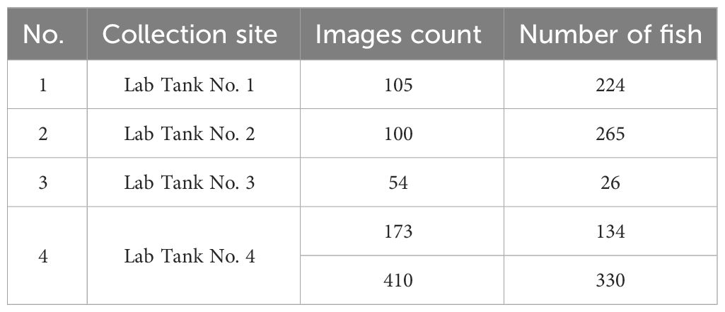
The data were collected from four fish tanks, with tank No. 4 sampled twice. The number of fish in each pond varied, leading to the data being divided into five groups based on these counts. The groups were represented by 173, 105, 100, 410, and 54 images of fish counting, respectively. Each image was manually annotated using the LabelMe tool, with a frame extracted every five seconds from the video, totaling 842 images of fish schools. Three master's students took approximately three weeks to annotate the dataset, marking an estimated total of 205,806 fish. Detailed information about the dataset is presented in Table 1.

Table 1

Table 1 Description of the fish school counting dataset.

This research faced the complex challenge of determining the position and the count of fish within schools. To address this issue, a method of marking the center of each fish was employed (Figure 3A). For partially obscured fish, the central point of their most exposed part was marked as accurately as possible (Figures 3B–E), although a small portion of fish were too heavily obscured to be annotated (Figure 3F). Each annotation label recorded the position of the respective fish, and the number of labels in the images indicated the quantity of fish in the school.

Figure 3

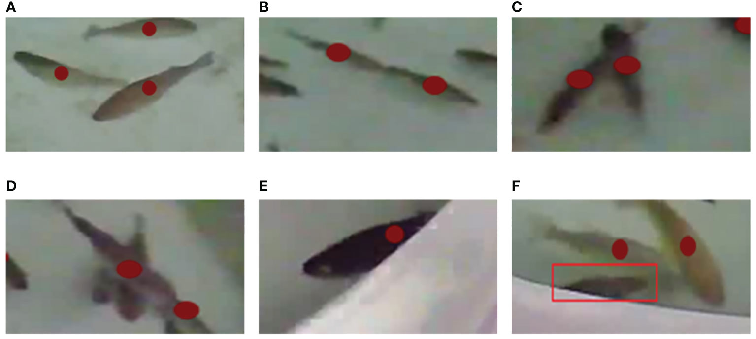
Figure 3 Examples of image annotations. (A) No overlapping. (B) Two fish overlapping to form a line. (C) Two fish crossing in a V shape. (D) Two fish intersecting in a V shape. (E) Majority of fish body exposed and annotated. (F) Only a small part of fish body exposed and not annotated.

2.4 Real ocean data set

To investigate the generalization capabilities of the FCFormer model across diverse datasets and real-world scenarios, we deliberately selected additional datasets characterized by varied environmental conditions and fish species for evaluation. Furthermore, the capacity for generalization across distinct scenarios is critically imperative for the model's extensive deployment in the aquaculture industry, given that real-world conditions frequently surpass the complexity and variability encountered in laboratory or specific dataset contexts. The experimental video data utilized in this study were sourced from "Deep Blue No. 1," an offshore aquaculture cage located in the Yellow Sea of China, courtesy of Rizhao Wanze Feng Fisheries Co., Ltd. The aquaculture involved adult Atlantic salmon, with all collected videos comprising underwater footage of this species, as shown in Figure 4.

Figure 4

Figure 4 Underwater adult Atlantic salmon pictures.

3 Fish school density estimation and counting network

3.1 Network architecture

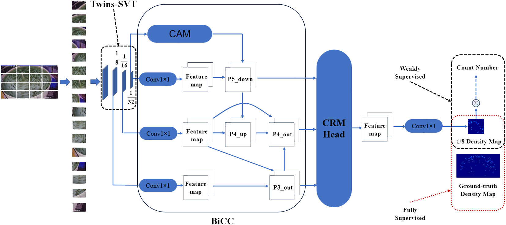
The entire process is systematically organized to effectively estimate the quantity of fish in the image, encompassing key steps including object detection, feature extraction, attention mechanisms, and density map regression. Initially, the input image is segmented into fixed-size image blocks. These blocks are subsequently flattened into a 1D sequence of vectors. Following this, the Twins-SVT backbone is employed to extract global features from the sequence. The extracted 1D sequences from each stage are then reshaped into 2D feature maps. To further refine the features, these 2D maps undergo feature extraction through a Weighted Bidirectional Feature Pyramid Network, coupled with a Class Activation Map module (BiCC). The refined features are subject to an element-wise summation. In the final stages, a CRMHead module is engaged to regress the density map. It is notable that FCFormer supports two supervision modes: in full-supervision mode, the regression result directly yields the density map, whereas in weak-supervision mode, the sum of all predicted pixel values in the density map is utilized as the fish count for regression. The model architecture, illustrating this comprehensive process, is depicted in Figure 5.

Figure 5

Figure 5 FCFormer network architecture.

3.1.1 2D image to 1D sequence

Prior to entering the Transformer backbone, the 2D image is reshaped into a 1D sequence. Following a similar image processing method as described in CCTrans (Tian et al., 2021), the input image is denoted as: $I\in R^{H\times W\times 3}$ (with H, W, and 3 representing height, width, and channel dimensions). Subsequently, it is divided into $K\times K$ image blocks, each sized at $\frac{H}{K}\times \frac{W}{K}\times 3$. These 2D image blocks are then seamlessly flattened into a 1D block sequence $x\in R^{N\times D}$ (where $N=\frac{H\times W}{K^2}\times 3$, $D=K\times K$). Next, a learnable projection, denoted as $f$: $xi\to ei\in R^D(i=1,\dots N)$, is applied to the sequence x to perform block embedding, resulting in the sequence $e\in R^{N\times D}$. As a result, the spatial and channel characteristics of the i-th image block, denoted as $x_i$, are transformed into the features of the i-th embedded vector, denoted as $e_i$.

3.1.2 Twins-SVT backbone

Twins-SVT combines local self-attention and global attention mechanisms, achieving image feature processing through the introduction of Spatially Separable Self-Attention (SSSA). SSSA comprises Local Spatial Attention (LSA) and Global Subsampling Attention (GSA), as illustrated in Figure 6. This combination enables the model to capture both local and global information simultaneously. By incorporating global attention after local self-attention, Twins-SVT addresses the issue of diminishing receptive fields while delivering exceptional performance in prediction tasks. Its notable advantages lie in its efficiency and ease of implementation, holding significant potential for application across various visual tasks.

Figure 6

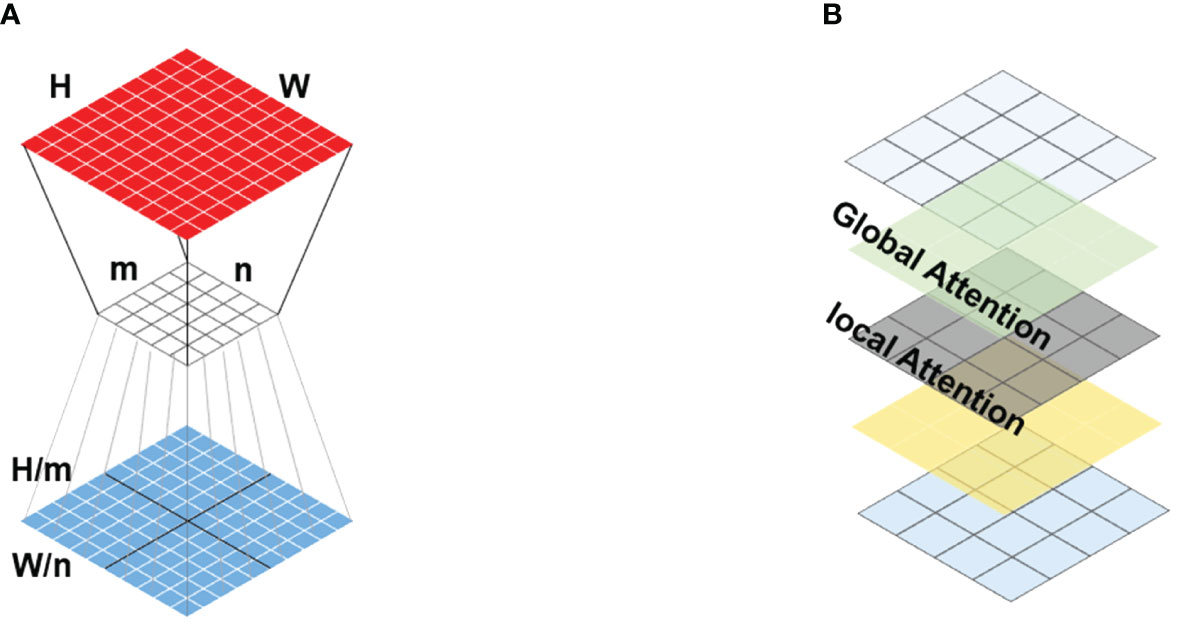
Figure 6 Channel attention structure diagram. (A) Twins-SVT interleaves locally-grouped attention (LSA) and global sub-sampled attention (GSA). (B) Schematic view of the locally-grouped attention (LSA) and global sub-sampled attention (GSA).

Formally, spatially separable self-attention (SSSA) can be expressed as Equations 1–4:

$\begin{array}{ll}{\dot{z}}_{ij}^l=LSA(LayerNorm(z_{ij}^{l-1}))+z_{ij}^{l-1}& (1)\end{array}$

$\begin{array}{ll}{z}_{ij}^l=FFN(LayerNorm({\dot{z}}_{ij}^l))+{\dot{z}}_{ij}^l& (2)\end{array}$

$\begin{array}{ll}{\dot{z}}^{l+1}=GSA(LayerNorm(z^l))+z^l& (3)\end{array}$

$\begin{array}{ll}{z}^{l+1}=FFN(LayerNorm({\dot{z}}^{l+1}))+{\dot{z}}^{l+1}& (4)\end{array}$

$$i\in \left\{1,2,\dots .,m\right\},j\in \left\{1,2\dots .,n\right\}$$

3.1.3 The Bi-FPN pyramid aggregation network with the CAM count module (Bicc)

Traditional feature pyramid networks typically adopt a unidirectional structure, either top-down or bottom-up, which can lead to the loss of crucial details or contextual information in information propagation and feature fusion. This limitation hampers their ability to effectively extract the contour information of objects like fish schools. In the backbone network, the frequent employment of down-sampling for deep feature extraction leads to a diminishment, or even disappearance, of the feature information of small objects as the feature hierarchy increases. To address these issues, this paper introduces a Bi-FPN aggregation network with the CAM module. In the backbone network, the top-level feature extraction layer is removed, a common choice in many studies (Li et al., 2018), which reduces network complexity while preventing irrelevant information from entering the subsequent channel feature fusion stage. Bi-FPN (Tan et al., 2020) incorporates a bidirectional, bottom-up, and top-down feature network structure. It introduces lateral connections between feature pyramids at each level, enabling feature information to flow freely within the network. This bidirectional connection design aids in better fusing features from different levels and maintaining a balance between low-level and high-level features.

To address the issue of different input features having varying degrees of influence on the output features at their respective resolutions, additional weights are introduced for each input feature. This allows the network to learn and quantify the importance of each feature. Building upon this concept, this paper employs a concise and efficient weighted feature fusion mechanism. There are three methods for weighted feature fusion: Unbounded fusion, SoftMax-based fusion, and Fast normalized fusion. In this case, Fast normalized fusion, a weighted feature fusion method, is chosen due to its fast-training speed, high efficiency and relative stability. It can be represented as:

$\begin{array}{ll}O={\displaystyle {\sum }_i}\frac{w_i}{ϵ+{\displaystyle {\sum }_j{w}_j}}{I}_i& (5)\end{array}$

Equation 5 defines the output $O$ as a weighted sum of the input vecto0r $I_i$, where the weights $w_i$ are assured to be non-negative, typically achieved through the application of a Rectified Linear Unit (ReLU) activation function. Additionally, to circumvent potential numerical instability caused by a zero denominator, a minuscule constant $ϵ$ (valued at 0.0001) is introduced. The normalized weights $\frac{w_i}{ϵ+{\displaystyle {\sum }_j{w}_j}}$ensure that their sum is unity, thereby permitting interpretation as a probability distribution.

We use Equations 6, 7 to describe the fusion of two features as illustrated in Figure 4:

$\begin{array}{ll}{p}_4\_up=Conv(\frac{w_1·b+w_2·resize(p_5\_down)}{w_1+w_2+ϵ})& (6)\end{array}$

$\begin{array}{ll}{p}_4\_out=Conv(\frac{w_1^{\prime }·b+w_2^{\prime }·p_4\_up+w_3^{\prime }·resize(p_3\_out)}{w_1^{\prime }+w_2^{\prime }+w_3^{\prime }+ϵ})& (7)\end{array}$

In this context, we have two features: 'p4_up,' representing the intermediate feature from the top-down channel, and 'p4_out,' representing the output feature from the bottom-up channel. The 'resize' operation is employed, which can encompass either down sampling or up sampling, to harmonize the resolutions of these features. The parameter 'w' and ' $w\text{'}$' are learned parameter utilized to discern the relative importance of distinct features during the fusion process. To enhance efficiency further, feature fusion is executed through depth wise separable convolutions, with batch normalization and activation functions introduced following each convolution operation.

While the aforementioned architecture significantly enhances the network's multi-scale representation capability, it does not fully consider potential conflicting information between features at different scales. The lack of contextual information can limit further performance improvement, especially concerning small objects, which are susceptible to interference from conflicting information. Therefore, this paper introduces an approach to inject the CAM module from top to bottom into the Bi-FPN to introduce contextual information. This CAM module employs dilated convolutions with different dilation rates to capture contextual information from various receptive fields. The specific structure is illustrated in Figure 7.

Figure 7

Figure 7 CAM module structure.

3.1.4 CRMHead

Taking inspiration from feature selection and the divide-and-conquer approach (Chen et al., 2021; Dai et al., 2021; Li et al., 2023), this paper introduces a Feature Adaptive Fusion Regression Head (CRMHead). The core idea of this method is to adaptively select the appropriate feature layers for targets of different scales. In essence, CRMHead aims to intelligently fuse the three feature layers in the FPN, allowing high-level features to focus on detecting large objects and low-level features to focus on detecting small objects. Two linear layers are then designed for regression, using 1x1 convolutions for local channel awareness, followed by BN (Batch Normalization) and ReLU (Rectified Linear Unit) layers. Similarly, global channel awareness is achieved by adding global pooling operations before local channel awareness. The formula for feature adaptive fusion is defined as Equations 8, 9:

$\begin{array}{ll}F=W(f_1{w}_1+f_2(1-w_1))+(1-W)(f_2{w}_2+f_3(1-w_2))& (8)\end{array}$

$\begin{array}{ll}{w}_i=Sig\mathrm{mod}(L(f_i)+G(f_{i+1}))& (9)\end{array}$

Here, $f_1$ , $f_2$, $f_3$ represent the three output feature maps obtained after fusion in the BiCC (Bi-FPN with CAM Count module) network. F represents the fused feature, $L(f_i)$ represents the local perception channel of $f_i$, and $G(f_{i+1})$ signifies the global perception channel.

3.2 loss function

Different loss functions are employed for strong supervision in density regression and weak supervision in count regression. Strong supervision entails reading the annotated positions of each fish in the density map. Weak supervision, on the other hand, involves solely reading the total number of fish in the fish school from the density map without the need to know the specific positions of each fish.

For the loss function in strong supervision, the DM_Count loss function (Wang et al., 2020a) is utilized, which comprises three components: counting loss, Optimal Transport (OT) loss, and Total Variation (TV) loss. The overall loss for a predicted density map D and its ground truth density map is expressed as Equation 10:

$\begin{array}{ll}\ell (z,\widehat{z})={\ell }_C(z,\widehat{z})+{\lambda }_1{\ell }_{OT}(z,\widehat{z})+{\lambda }_2\mid \mid z\mid {\mid }_1{\ell }_{TV}(z,\widehat{z})& (10)\end{array}$

Here, $z$and $\widehat{z}$represent the fish counts in $D$and $D^{\text{'}}$, ${\lambda }_1$and ${\lambda }_2$are the loss coefficients, $\mid \mid z\mid {\mid }_1$denotes the vector norm of ${\ell }_{TV}$, In the experimental process, ${\lambda }_1$is set to 0.1, ${\lambda }_2$is set to 0.01.

For the loss function in weak supervision, a smooth ${\ell }_1$loss is used as a replacement for ${\ell }_1$loss. Due to significant variations in fish school counts across different images and the sensitivity of ${\ell }_1$to outliers, the weak supervision loss function is defined as Equation 11:

$\begin{array}{ll}{\ell }_C=smoot{h}_{{\ell }_C}(D,D^{\text{'}})& (11)\end{array}$

3.3 Evaluation metrics

The experiment uses Mean Absolute Error (MAE), Mean Squared Error (MSE), Mean Absolute Percentage Error (NAE), and accuracy to measure the performance of the proposed network. MAE and MSE are common metrics used to evaluate the performance of prediction networks, typically in regression problems. MAE is one of the most basic evaluation metrics, representing the average absolute error between predicted values and actual values, reflecting the accuracy of the estimation. MSE is the average of the squared differences between predicted and actual values, where larger errors in training affect MSE, making it a measure of the network’s stability. NAE (Wang et al., 2020b), considers not only the error between the predicted and actual values but also the error in relation to the actual values, offering a more comprehensive evaluation of network performance. Accuracy directly reflects the network’s performance under simplified conditions. These are represented by Equations 12–15:

$\begin{array}{ll}MAE=\frac{1}{N}{\displaystyle \sum _{i=1}^N\mid P_i}-G_i\mid & (12)\end{array}$

$\begin{array}{ll}MSE=\sqrt{\frac{1}{N}{\displaystyle \sum _{i=1}^N\mid P_i-G_i{\mid }^2}}& (13)\end{array}$

$\begin{array}{ll}NAE=\frac{1}{N}{\displaystyle \sum _{i=1}^N\frac{\mid P_i-G_i\mid }{G_i}}& (14)\end{array}$

$\begin{array}{ll}Accuracy=(1-\frac{100}{N}{\displaystyle \sum _{i=1}^N\frac{\mid P_i-G_i\mid }{G_i}})& (15)\end{array}$

Here, N is the number of images tested, $P_i$is the predicted number of fish in the i-th image, and $G_i$is the actual number of fish in the i-th image.

4 Experimental and discussion

4.1 Training parameter configuration

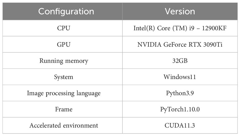
To substantiate the efficacy of the proposed algorithm, all computational experiments were executed with consistent hyperparameters. These encompassed a mini-batch size of 12 to leverage the stochastic gradient descent, utilization of the Adam optimization algorithm with weight decay regularization to facilitate sparse convergence, a fine-tuned learning rate of 1e-5 for precise gradient updates, and an extensive training duration across 1000 epochs to ensure robust model generalization. The precise configurations of the computational resources, including the high-performance CPU and GPU specifications, expansive memory capacity, and the software environment tailored for deep learning tasks, are comprehensively delineated in Table 2.

Table 2

Table 2 Lab environment.

4.2 Results analysis

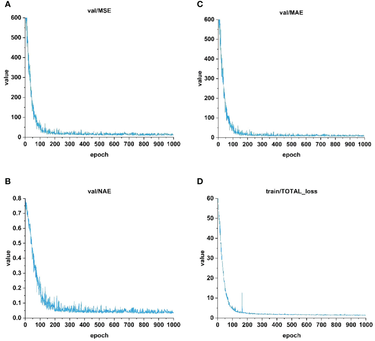
In order to comprehensively evaluate the effectiveness of the FCFormer model proposed in this paper, we analyze the performance of the model in the training and verification process in detail, with particular attention to the model’s ability to handle different density fish scenes. Figures 7, 8 and Table 3 show the key indicators of model performance, including the changes of MAE, MSE, NAE and loss values, as well as the performance of the model in different density scenarios.

Figure 8

Figure 8 Curve changes of MAE, MSE, NAE and loss. (A) MSE. (B) MAE. (C) NAE. (D) Loss.

Table 3

Table 3 Experimental results at different densities.

Figure 8 illustrates the variations in MAE, MSE, NAE, and loss curves during the validation and training processes. In the initial stages of the model, the metrics and loss values on the validation set were relatively high but started to decrease sharply after several training epochs. By the time 90 training iterations were completed, the MAE, MSE, NAE values, and loss had stabilized. Up to 1000 iterations, with increasing epochs, the errors exhibited slow oscillations and approached stability. The final MAE, MSE, and NAE values were 6.37, 8.69, and 2.94, respectively. However, due to the inherent complexity of the dataset, further error reduction became challenging. As the errors gradually decreased and stabilized, the model converged, yielding training results in line with expectations.

The performance of FCFormer under different density scenarios is outlined in Table 3. It is evident that FCFormer performs exceptionally well in sparse and moderate-density scenarios, exhibiting lower MAE and MSE along with higher accuracy. However, detecting fish schools in slightly denser scenarios poses a greater challenge. This challenge arises as such scenarios feature a significant number of smaller-sized and occluded fish targets, potentially obstructing effective feature extraction. Despite these challenges, FCFormer continues to showcase commendable detection performance even as the number of fish schools increases, attributed to BiCC’s effective extraction of more detailed information.

The trained model is used to generate high-quality fish school density maps, with the final density maps being 1/8 of the original images. Figure 9 displays a set of relatively poorer results and five sets of relatively better results. Apart from the counting results, the five sets of predicted density maps closely match the ground truth density maps, providing an overall representation of the fish school distribution. However, there are still a few instances of poorer results in the experimental outcomes. Upon analysis, it was found that severe occlusion of some fish schools and mislabeling issues in the test samples, such as omissions or incorrect annotations, contributed to these challenges. Addressing these labeling issues can further enhance the model’s robustness and accuracy.

Figure 9

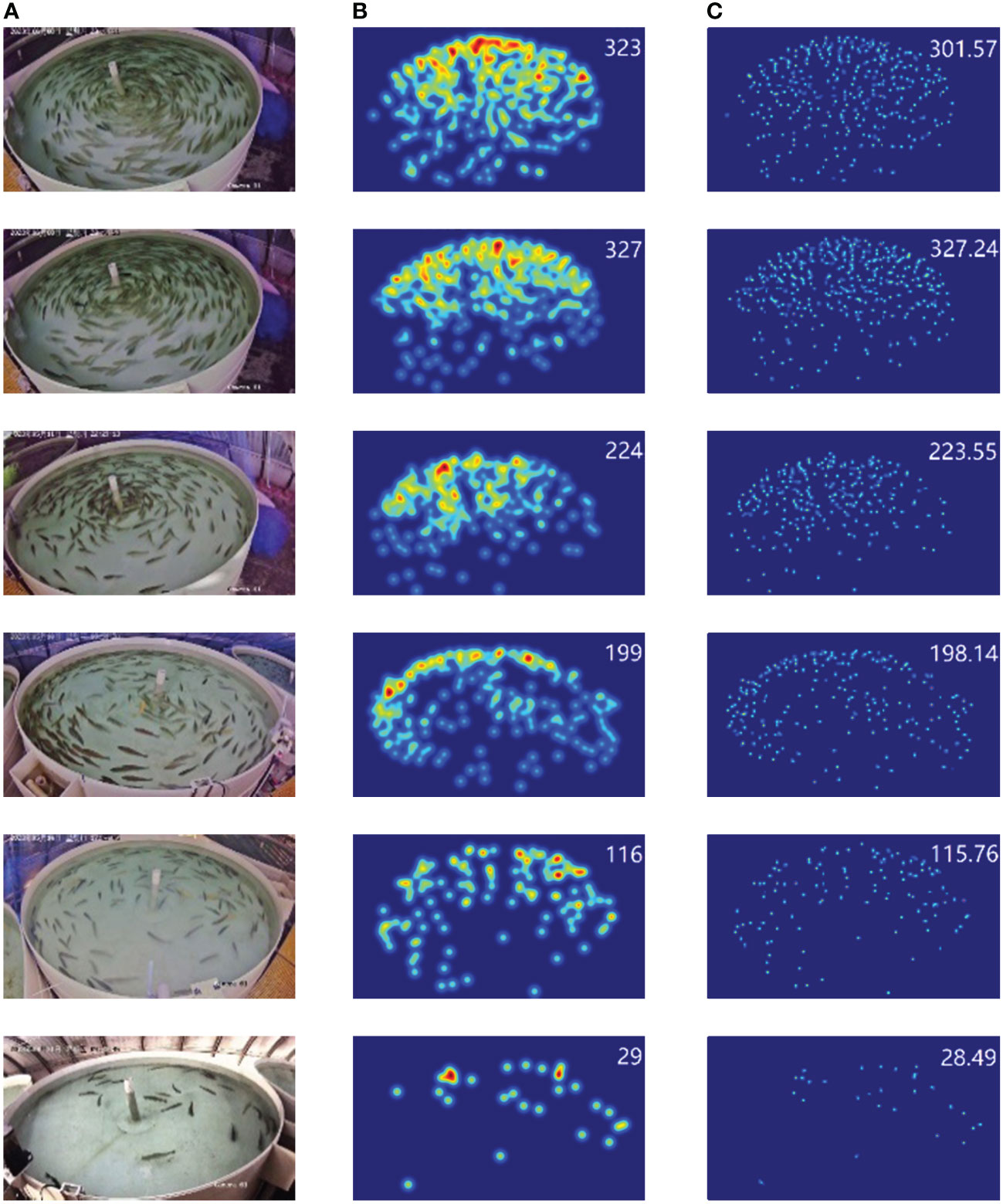
Figure 9 Fish count results and density plots. (A) Original image. (B) Ground truth. (C) Prediction.

4.3 Comparison with other networks

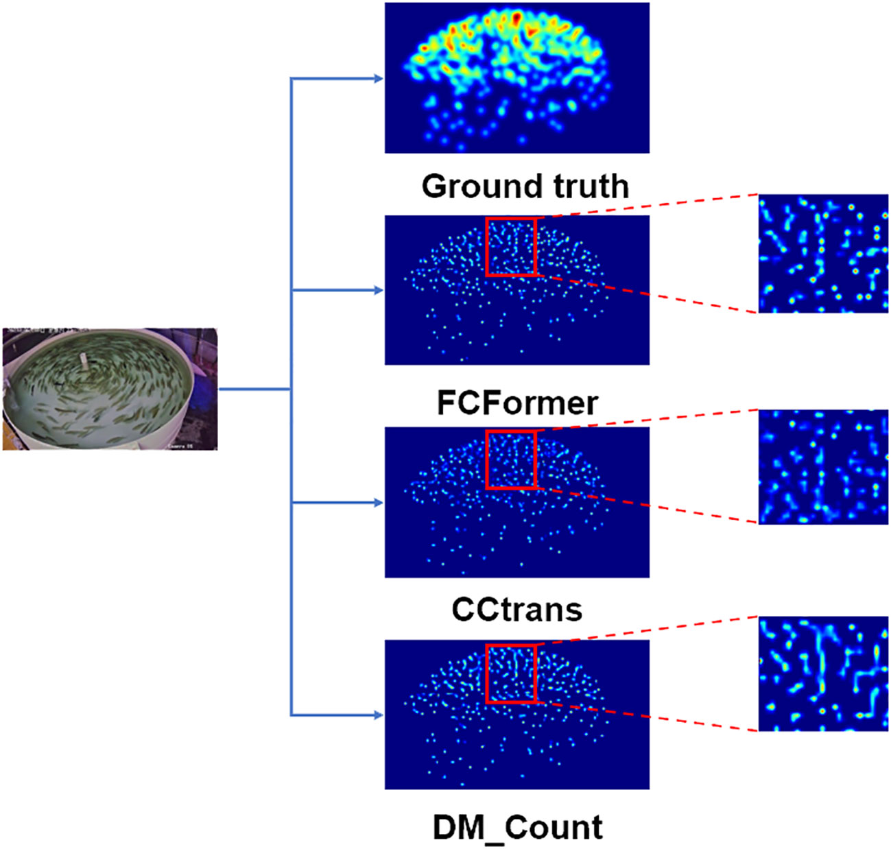
The quality comparison of the density maps is shown in Figure 10. Clearly, FCFormer produces higher-quality density maps with a stronger capability to extract features of tiny fish targets in the distance. This is attributed to the CAM module that integrates multi-scale dilated convolution features, enabling the acquisition of rich contextual information for feature enhancement.

Figure 10

Figure 10 Comparison of the quality of density maps generated by different models.

The trained model is used to generate high-quality fish school density maps, with the density map size matching that of the corresponding input images. Density map predictions were made for five groups of fish schools at different densities and compared to the ground truth density maps. Additionally, the density predictions from the FCFormer model were compared with those from CCTrans and DM_Count. The quality comparison results of the density maps are shown in Figure 11. Figures 11A and B display original fish images from five different density levels along with their corresponding ground truth. Figure 11C–E show the respective predicted density maps generated by FCFormer, CCTrans, and DM_Count, Respectively, the ground truth values and model predictions are displayed in the upper right corner of the density maps. The results indicate that under various density scenarios, the predicted density maps by all models exhibit good accuracy and accurately reflect the distribution of fish school density. This highlights the feasibility of density map regression-based methods in fish counting. Furthermore, the density maps generated by FCFormer closely resemble the ground truth, attributed to BiCC’s effective extraction of more detailed information.

Figure 11

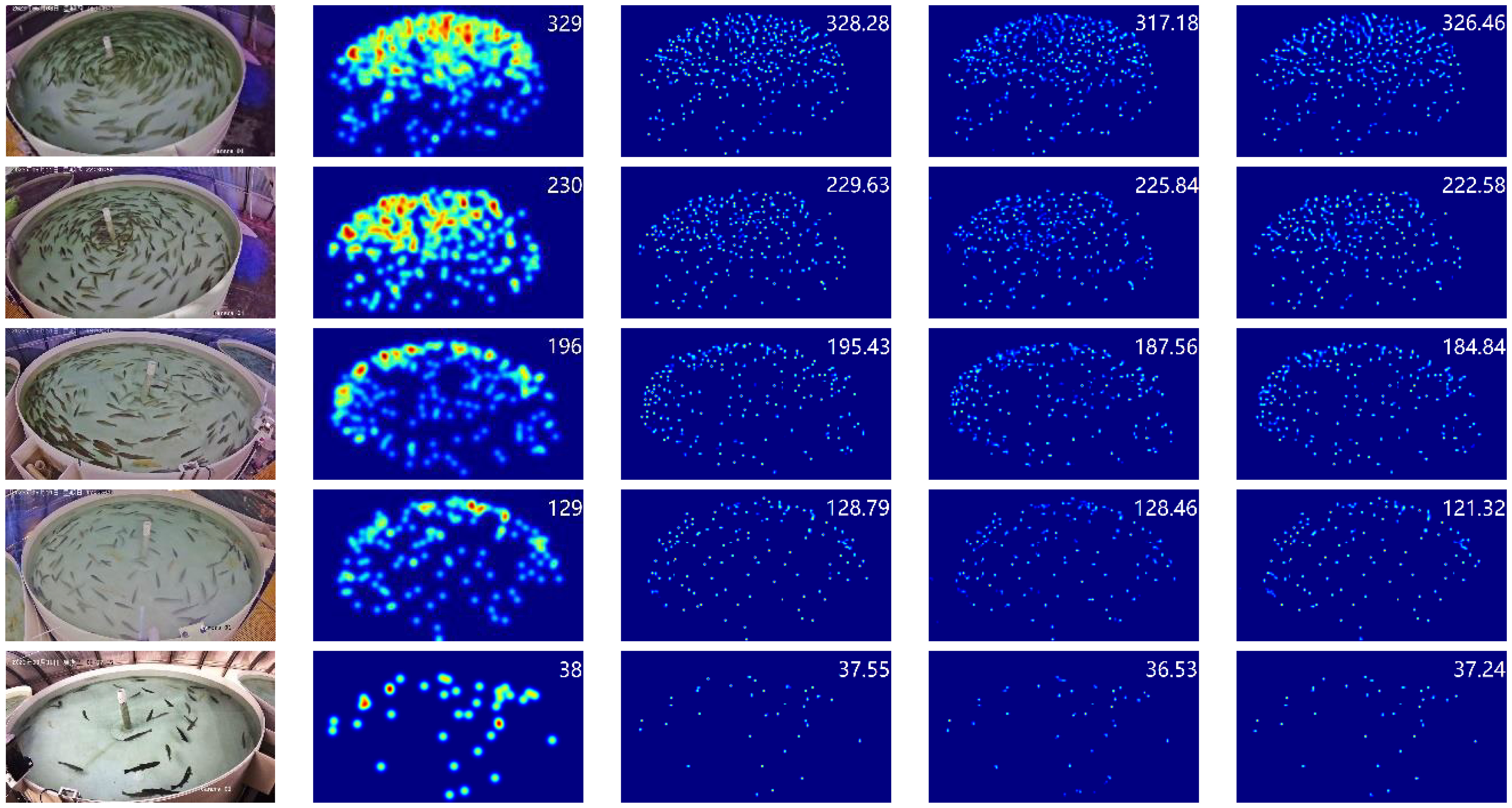
Figure 11 Fish counting results and density maps of different densities for each model. (A) Original image. (B) Ground truth. (C) FCFormer. (D) CCTrans. (E) DM_Count.

To provide a more intuitive representation of FCFormer’s counting performance, an error analysis was conducted between the model predictions and ground truth values for FCFormer, DM_Count, and CCTrans on 278 test images. As shown in the box plot in Figure 12A, the two black short lines outside the red box represent the maximum and minimum error values, the top and bottom of the box represent the upper and lower quartiles, and the middle line is the median line. The “×” represents the average value marker. It can be observed that FCFormer has the lowest upper and lower bounds for errors, and both the quartiles and the average value are the smallest. Figure 12B shows that 77% of the errors remain within the range of -10 to 10, indicating that FCFormer has low data fluctuations and excellent stability. Therefore, FCFormer outperforms other methods in terms of stability and accuracy.

Figure 12

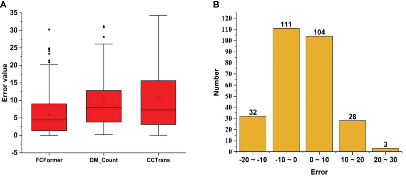
Figure 12 Error analysis between network prediction results and Ground truth. (A) Box plot comparison results of each networks test (B) FCFormer error ratio graph between real value and estimated value.

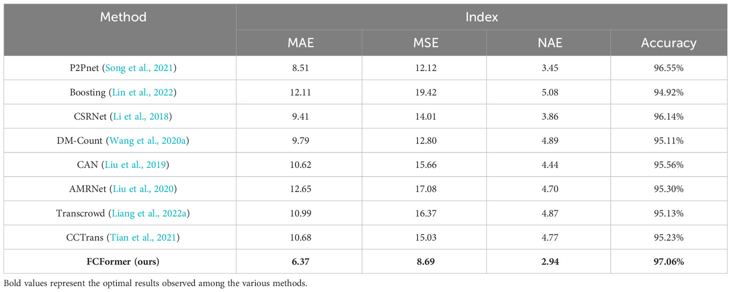
To validate the performance of various fish school counting models, this study selected multiple models for comparative analysis of methods and accuracy. The prediction results of each model are shown in Table 4. The proposed fish school counting method based on FCFormer outperforms other comparative methods. Compared to two other transformer-based models, CCTrans and TransCrowd, FCFormer achieved an improvement in counting accuracy of 2.09% and 2.19%, respectively. This indicates a clear advantage of the proposed research method.

Table 4

Table 4 Comparative experiment.

4.4 Ablation study results analysis

In this paper, ablation experiments were conducted on the CRMHead module①, Bi-FPN②, and CAM module③, as shown in Figures 13A, B, and Table 5. Twins-SVT was chosen as the baseline model, which achieved an accuracy of 95.04%. When the CRMHead module, Bi-FPN, and CAM module were sequentially added, the model’s accuracy reached 97.06%. The results indicate that each added module played a role in improving accuracy.

Figure 13

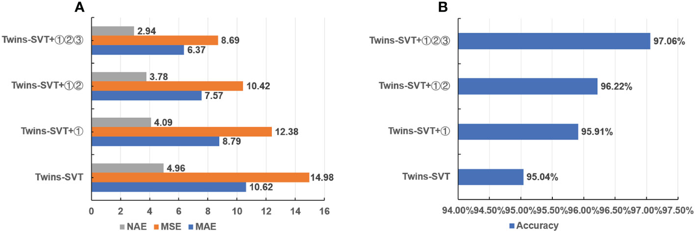
Figure 13 Comparison chart of ablation experiments. (A) Ablation experiment NAE, MSE, MAE comparison chart. (B) Ablation experiment accuracy comparison chart.

Table 5

Table 5 FCFormer ablation experiment.

4.5 Supplementary experiment

In the testing of the FCFormer model within the “Deep Blue No.1” aquaculture net cage, the experimental results are shown in Table 6, demonstrating the model’s high precision and minimal error. These results substantiate FCFormer’s robust generalization capabilities and its potential applicability in authentic aquaculture settings. As illustrated in Figure 14, the generated density maps provide a clear visualization of the model’s capacity to accurately identify and count Atlantic salmon amidst complex backgrounds and under varying lighting conditions. Collectively, these findings affirm that the FCFormer model not only excels on benchmark datasets but also its high accuracy and low error rates in real-world application scenarios further validate the model’s generalization capacity and the feasibility of its practical implementation.

Table 6

Table 6 The experimental results of FCFormer on real ocean data sets.

Figure 14

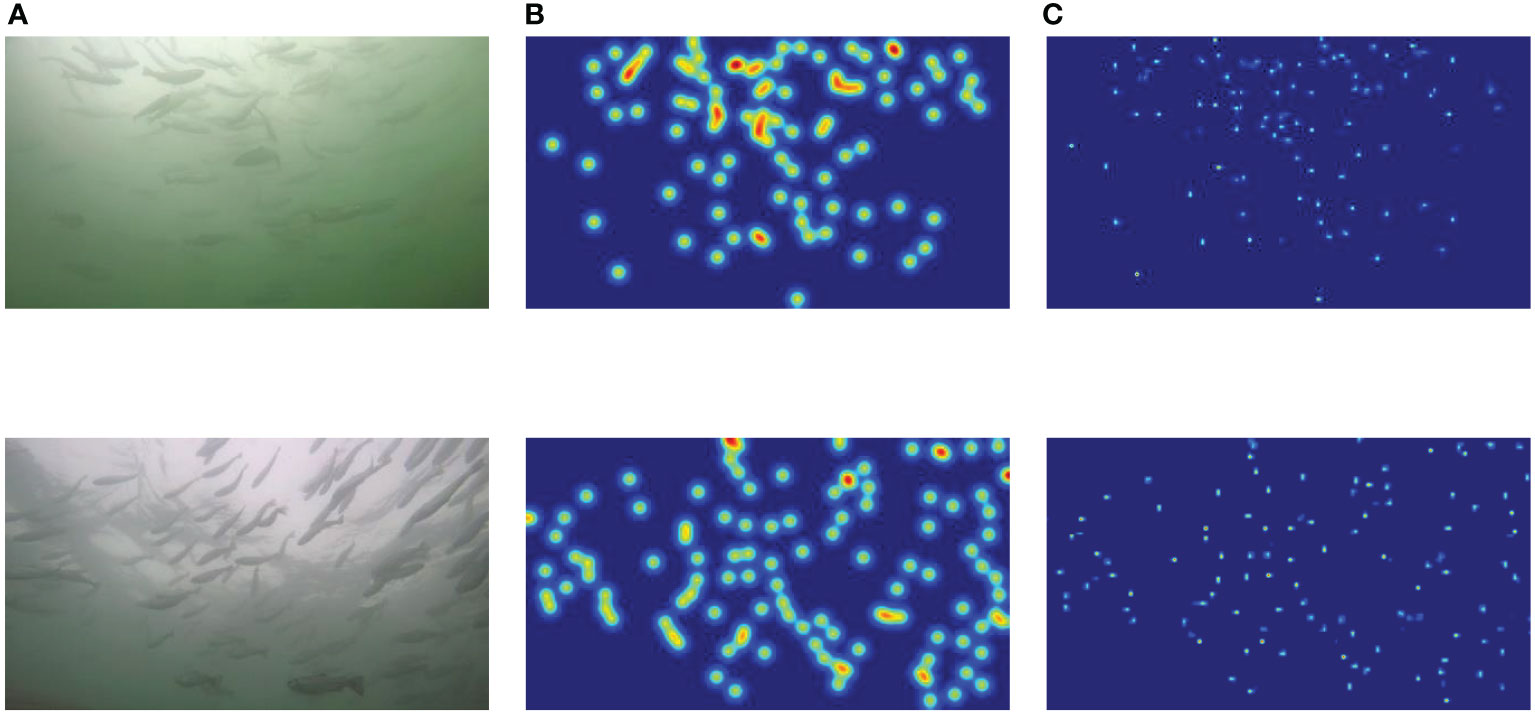
Figure 14 Adult Atlantic salmon count results and density plots. (A) Original image. (B) Ground truth. (C) Prediction.

4.6 Future works

While FCFormer has achieved good results in fish school counting, there are several areas for improvement in this study:

(1) Due to experimental constraints, the dataset had a relatively uniform and single background, collected from only four fish tanks. To enhance the algorithm’s robustness, it is necessary to conduct more experiments in a wider range of fish tanks and more complex background environments.

(2) Despite FCFormer’s performance being superior to other comparative methods, there is still room for improvement. Future efforts should focus on addressing occlusion issues.

(3) Given the practical applications of counting tasks, it could be beneficial to validate FCFormer’s effectiveness in a broader ecosystem to further demonstrate the model’s generality and adaptability.

(4) Although FCFormer performs well on specific data sets, in practical applications, especially in real-time monitoring or management of ecosystems, the deployment of models is crucial. In the future, we will explore model compression and acceleration techniques so that FCFormer can run efficiently on resource-constrained devices and meet the requirements of real-time processing.

5 Conclusion

In response to the challenges posed by fish school detection and the recognition of distant small targets, this paper proposed a fish school detection algorithm, FCFormer, based on density map regression. The design incorporated a BiCC aggregation network with a CAM Count module, which not only enhanced the fusion of low-level and high-level features but also significantly improved the quality of the density maps by extracting better features. Subsequently, efficient regression counting model CRMHead was employed for density map prediction, resulting in an accuracy rate of 97.06% for FCFormer. This represented a 2.02% improvement over the Twins transformer baseline and outperformed other comparative models. Moreover, this model demonstrated excellent applicability and could be applied in intelligent feeding recirculating aquaculture systems, providing a reliable algorithmic reference for precise fish school counting.

Data availability statement

The raw data supporting the conclusions of this article will be made available by the authors, without undue reservation.

Author contributions

KZ: Conceptualization, Formal analysis, Investigation, Methodology, Software, Writing – original draft. XY: Data curation, Writing – original draft. CY: Investigation, Visualization, Writing – original draft. TF: Resources, Supervision, Writing – original draft. PM: Software, Validation, Writing – original draft. WH: Data curation, Visualization, Writing – original draft.

Funding

The author(s) declare financial support was received for the research, authorship, and/or publication of this article. The research was funded by the National Key Research and Development Program of China (2022YFD2001701), the National Natural Science Foundation of China (32373184), the Beijing Natural Science Foundation, China (6212007).

Conflict of interest

The authors declare that the research was conducted in the absence of any commercial or financial relationships that could be construed as a potential conflict of interest.

Publisher’s note

All claims expressed in this article are solely those of the authors and do not necessarily represent those of their affiliated organizations, or those of the publisher, the editors and the reviewers. Any product that may be evaluated in this article, or claim that may be made by its manufacturer, is not guaranteed or endorsed by the publisher.

References

Abe S., Takagi T., Torisawa S., Abe K., Habe H., Iguchi N., et al. (2021). Development of fish spatio-temporal identifying technology using segnet in aquaculture net cages. Aquac. Eng. 93, 102146. doi: 10.1016/j.aquaeng.2021.102146

CrossRef Full Text | Google Scholar

Albuquerque P. L. F., Garcia V., Junior A. D. S. O., Lewandowski T., Detweiler C., Gonçalves A. B., et al. (2019). Automatic live fingerlings counting using computer vision. Comput. Electron Agric. 167, 105015. doi: 10.1016/j.compag.2019.105015

CrossRef Full Text | Google Scholar

Awalludin E., Muhammad W. W., Arsad T., Yussof W. H. W. (2020). Fish larvae counting system using image processing techniques. J. Of Physics: Conf. Ser. 1529, 052040. doi: 10.1088/1742-6596/1529/5/052040

CrossRef Full Text | Google Scholar

Babu K. M., Bentall D., Ashton D. T., Puklowski M., Fantham W., Lin H. T., et al. (2023). Computer vision in aquaculture: A case study of juvenile fish counting. J. R Soc. N Z 53, 52–68. doi: 10.1080/03036758.2022.2101484

CrossRef Full Text | Google Scholar

Chen Q., Wang Y., Yang T., Zhang X., Cheng J., Sun J. (2021). “You only look one-level feature,” in Proceedings Of The Ieee/Cvf Conference On Computer Vision And Pattern Recognition. IEEE 13039–13048.

Google Scholar

Chu X., Tian Z., Wang Y., Zhang B., Ren H., Wei X., et al. (2021). Twins: revisiting the design of spatial attention in vision transformers. Adv. Neural Inf Process Syst. 34, 9355–9366. doi: 10.48550/Arxiv.2104.13840

CrossRef Full Text | Google Scholar

Dai Y., Gieseke F., Oehmcke S., Wu Y., Barnard K. (2021). “Attentional feature fusion,” in Proceedings Of The Ieee/Cvf Winter Conference On Applications Of Computer Vision. IEEE 3560–3569.

Google Scholar

Fabic J., Turla I., Capacillo J., David L., Naval P. (2013). “Fish population estimation and species classification from underwater video sequences using blob counting and shape analysis,” in 2013 Ieee International Underwater Technology Symposium (Ut). 1–6 (Tokyo,Japan: Ieee).

Google Scholar

Feng S., Yang X., Liu Y., Zhao Z., Liu J., Yan Y., et al. (2022). Fish feeding intensity quantification using machine vision and A lightweight 3d resnet-glore network. Aquac. Eng. 98, 102244. doi: 10.1016/j.aquaeng.2022.102244

CrossRef Full Text | Google Scholar

Kamilaris A., Prenafeta-Boldú F. X. J. C., Agriculture E. I. (2018). Deep learning in agriculture: A survey. Comput. Electron Agric. 147, 70–90. doi: 10.1016/j.compag.2018.02.016

CrossRef Full Text | Google Scholar

Labuguen R., Volante E., Causo A., Bayot R., Peren G., Macaraig R., et al. (2012). “Automated fish fry counting and schooling behavior analysis using computer vision,” in 2012 Ieee 8th International Colloquium On Signal Processing And Its Applications. 255–260 (Malacca,Malaysia: Ieee).

Google Scholar

Lainez S. M. D., Gonzales D. B. (2019). “Automated fingerlings counting using convolutional neural network,” in 2019 Ieee 4th International Conference On Computer And Communication Systems (Icccs). 67–72 (Singapore: Ieee).

Google Scholar

Lecun Y., Bengio Y., Hinton G. J. N. (2015). Deep learning. Nature 521, 436–444. doi: 10.1038/nature14539

PubMed Abstract | CrossRef Full Text | Google Scholar

Li D., Hao Y., Duan Y. J. R. I. A. (2020). Nonintrusive methods for biomass estimation in aquaculture with emphasis on fish: A review. Rev. Aquac 12, 1390–1411. doi: 10.1111/raq.12388

CrossRef Full Text | Google Scholar

Li Z., Liu F., Yang W., Peng S., Zhou J. J. I. T. O. N. N., Systems L. (2021b). A survey of convolutional neural networks: analysis, applications, and prospects. IEEE Trans. Neural Netw. Learn Syst. 33, 6999–7019. doi: 10.1109/TNNLS.2021.3084827

CrossRef Full Text | Google Scholar

Li D., Miao Z., Peng F., Wang L., Hao Y., Wang Z., et al. (2021a). Automatic counting methods in aquaculture: A review. J. World Aquac Soc. 52, 269–283. doi: 10.1111/jwas.12745

CrossRef Full Text | Google Scholar

Li Y., Zhang X., Chen D. (2018). “Csrnet: dilated convolutional neural networks for understanding the highly congested scenes,” in Proceedings Of The Ieee Conference On Computer Vision And Pattern Recognition. Salt Lake City, UT: IEEE 1091–1100.

Google Scholar

Li B., Zhang Y., Xu H., Yin B. J. T. V. C. (2023). Ccst: crowd counting with swin transformer. Vis. Comput. 39, 2671–2682. doi: 10.1007/s00371-022-02485-3

CrossRef Full Text | Google Scholar

Liang D., Chen X., Xu W., Zhou Y., Bai X. J. S. C. I. S. (2022a). Transcrowd: weakly-supervised crowd counting with transformers. Sci. China Life Sci. 65, 160104. doi: 10.1007/s11432-021-3445-y

CrossRef Full Text | Google Scholar

Liang D., Xu W., Bai X. (2022b). An end-to-end transformer model for crowd localization. Eur. Conf. On Comput. Vision 13661, 38–54. doi: 10.1007/978-3-031-19769-7_3

CrossRef Full Text | Google Scholar

Liao W., Zhang S., Wu Y., An D., Wei Y. J. A. E. (2022). Research on intelligent damage detection of far-sea cage based on machine vision and deep learning. Aquac. Eng. 96, 102219. doi: 10.1016/j.aquaeng.2021.102219

CrossRef Full Text | Google Scholar

Lin H., Ma Z., Ji R., Wang Y., Hong X. (2022)Boosting crowd counting via multifaceted attention (Accessed Proceedings Of The Ieee/Cvf Conference On Computer Vision And Pattern Recognition). doi: 10.1109/CVPR52688.2022.01901

CrossRef Full Text | Google Scholar

Liu W., Salzmann M., Fua P. (2019). “Context-aware crowd counting,” in Proceedings Of The Ieee/Cvf Conference On Computer Vision And Pattern Recognition. Long Beach, CA, USA: IEEE 5099–5108.

Google Scholar

Liu X., Yang J., Ding W., Wang T., Wang Z., Xiong J. (2020). “Adaptive mixture regression network with local counting map for crowd counting,” in Computer Vision–Eccv 2020: 16th European Conference, Glasgow, Uk, August 23–28, 2020, Proceedings, Part Xxiv 16. 241–257 (Glasgow, UK: Springer).

Google Scholar

Mo H., Ren W., Zhang X., Yan F., Zhou Z., Cao X., et al. (2022). Attention-guided collaborative counting. IEEE Trans. Image Process 31, 6306–6319. doi: 10.1109/TIP.2022.3207584

PubMed Abstract | CrossRef Full Text | Google Scholar

Morais E. F., Campos M. F. M., Pádua F. L., Carceroni R. L. (2005). “Particle filter-based predictive tracking for robust fish counting,” in Xviii Brazilian Symposium On Computer Graphics And Image Processing (Sibgrapi’05). 367–374 (Natal, Brazil: Ieee).

Google Scholar

Puig-Pons V., Muñoz-Benavent P., Espinosa V., Andreu-García G., Valiente-González J. M., Estruch V. D., et al. (2019). Automatic bluefin tuna (Thunnus thynnus) biomass estimation during transfers using acoustic and computer vision techniques. Aquac. Eng. 85, 22–31. doi: 10.1016/j.aquaeng.2019.01.005

CrossRef Full Text | Google Scholar

Říha M., Prchalová M., Brabec M., Draštík V., Muška M., Tušer M., et al. (2023). Calibration of fish biomass estimates from gillnets: step towards broader application of gillnet data. Ecol. Indic 153, 110425. doi: 10.1016/j.ecolind.2023.110425

CrossRef Full Text | Google Scholar

Song Q., Wang C., Jiang Z., Wang Y., Tai Y., Wang C., et al. (2021). “Rethinking counting and localization in crowds: A purely point-based framework,” in Proceedings Of The Ieee/Cvf International Conference On Computer Vision. Montreal, QC ,Canada: IEEE 3365–3374.

Google Scholar

Tan M., Pang R., Le Q. V. (2020). “Efficientdet: scalable and efficient object detection,” in Proceedings Of The Ieee/Cvf Conference On Computer Vision And Pattern Recognition. Seattle, WA, USA: IEEE 10781–10790.

Google Scholar

Tian Y., Chu X., Wang H. (2021). “Cctrans: simplifying and improving crowd counting with transformer,” in Cvpr. doi: 10.48550/Arxiv.2109.14483

CrossRef Full Text | Google Scholar

Toh Y., Ng T., Liew B. (2009). “Automated fish counting using image processing,” in 2009 International Conference On Computational Intelligence And Software Engineering. 1–5 (Wuhan, China: Ieee).

Google Scholar

Vaswani A., Shazeer N., Parmar N., Uszkoreit J., Jones L., Gomez A. N., et al. (2017). Attention is all you need. Adv. Neural Inf Process Syst. 30. doi: 10.48550/Arxiv.1706.03762

CrossRef Full Text | Google Scholar

Wang Q., Gao J., Lin W., Li X., Intelligence M. (2020b). Nwpu-crowd: A large-scale benchmark for crowd counting and localization. IEEE Trans. Pattern Anal. Mach. Intell. 43, 2141–2149. doi: 10.1109/TPAMI.34

CrossRef Full Text | Google Scholar

Wang B., Liu H., Samaras D., Nguyen M. H. (2020a). Distribution matching for crowd counting. Adv. Neural Inf Process Syst. 33, 1595–1607. doi: 10.48550/Arxiv.2009.13077

CrossRef Full Text | Google Scholar

Xiao R., Wei Y., An D., Li D., Ta X., Wu Y., et al. (2018). A review on the research status and development trend of equipment in water treatment processes of recirculating aquaculture systems. Rev. In Aquacul. 11, 863–895. doi: 10.1111/raq.12270

CrossRef Full Text | Google Scholar

Yu X., Wang Y., An D., Wei Y. J. A. E. (2022). Counting method for cultured fishes based on multi-modules and attention mechanism. Aquac. Eng. 96, 102215. doi: 10.1016/j.aquaeng.2021.102215

CrossRef Full Text | Google Scholar

Zeng Y., Yang X., Pan L., Zhu W., Wang D., Zhao Z., et al. (2023). Fish school feeding behavior quantification using acoustic signal and improved swin transformer. Comput. Electron Agric. 204, 107580. doi: 10.1016/j.compag.2022.107580

CrossRef Full Text | Google Scholar

Zhang L., Li W., Liu C., Zhou X., Duan Q. J. C., Agriculture E. I. (2020a). Automatic fish counting method using image density grading and local regression. Comput. Electron Agric. 179, 105844. doi: 10.1016/j.compag.2020.105844

CrossRef Full Text | Google Scholar

Zhang S., Yang X., Wang Y., Zhao Z., Liu J., Liu Y., et al. (2020b). Automatic fish population counting by machine vision and A hybrid deep neural network model. Animals 10, 364. doi: 10.3390/ani10020364

PubMed Abstract | CrossRef Full Text | Google Scholar

Zhao Y., Li W., Li Y., Qi Y., Li Z., Yue J. J. C., et al. (2022). Lfcnet: A lightweight fish counting model based on density map regression. Comput. Electron Agric. 203, 107496. doi: 10.1016/j.compag.2022.107496

CrossRef Full Text | Google Scholar

Zhao J., Li Y., Zhang F., Zhu S., Liu Y., Lu H., et al. (2018). Semi-supervised learning-based live fish identification in aquaculture using modified deep convolutional generative adversarial networks. T Asabe 61, 699–710. doi: 10.13031/trans.12684

CrossRef Full Text | Google Scholar

Zhou J., Ji D., Zhao J., Zhu S., Peng Z., Lu G., et al. (2022). A kinematic analysis-based on-line fingerlings counting method using low-frame-rate camera. Comput. Electron Agric. 199, 107193. doi: 10.1016/j.compag.2022.107193

CrossRef Full Text | Google Scholar

Zion B. J. C., Agriculture E. I. (2012). The use of computer vision technologies in aquaculture–A review. Comput. Electron Agric. 88, 125–132. doi: 10.1016/j.compag.2012.07.010

CrossRef Full Text | Google Scholar