Evaluation of beach response due to construction of submerged detached breakwater

Submerged detached breakwaters (SDBWs) have increasingly been used in recent times as an alternative against their emergent counterpart (EDBWs) to mitigate erosion because the former do not spoil the seascape. Both of these structures are (usually) constructed using precast concrete blocks or natural granite rocks, hence becoming permeable structures. For an EDBW, a parabolic bay shape equation can be readily used to estimate the planar shape of the shoreline behind the structure, but there is still no approach to estimate how the shoreline behind the SDBW is formed. In this study, we estimated how the shoreline is balanced by examining how the dominant wave direction changes due to the diffraction of the transmitted wave generated after the installation of the SDBW from the long-term wave directional spectrum. The change in dominant wave direction was determined under the shoreline gradient condition where littoral drift does not occur, considering the diffraction phenomenon due to the difference in transmitted waves. This means that the shape of the equilibrium shoreline changes to face perpendicular to the dominant wave direction. As a meaningful result, when the transmittance is 0, it converges to the well-known empirical equation of EDBW. The present methodology is validated by comparing the observed data (wave and shoreline change) from two beaches (Anmok and Bongpo-Cheonjin Beaches) on the eastern coast of Korea. This rational approach to shoreline changes behind permeable SDBWs will help in proactive review work for coastal management as well as beach erosion mitigation.

1 Introduction

Historically, coasts were used mainly for fishing and playing on the beach. Nowadays, it has become an important place that focuses on coastal functionalities such as habitat and recreation. For these reasons, coastal structures are being built on many beaches to protect these coastal functionalities. However, while the protective structures are favorable, they have often adversely caused beach erosion, in addition to reckless development projects and climate change that may have contributed to accelerating beach erosion. Therefore, diverse countermeasures should be provided to reduce beach erosion (Lim et al., 2021b).

Recently, submerged detached breakwaters (SDBWs) have been constructed instead of emergent detached breakwaters (EDBWs) to mitigate beach profile erosion, to conserve the beach landscape. Thus, a critical requirement has arisen for researching how these structures affect shoreline changes. In this paper, permeable SDBWs that can partially reflect and transmit waves are tentatively referred to as permeable structures to ease the task of analysis.

Coastal structures, such as SDBWs and EDBWs, are built to reduce incident wave energy and to protect the beach from wave action. Theoretically, Wang et al. (1975) proposed the shoreline response (i.e., advance or retreat) caused by incident waves. A shoreline evolution model was first proposed by Wright and Short (1984) using an empirical approach that relies on disequilibrium beach states and relative wave energy. Yates et al. (2009) conducted long-term field observations to obtain a general understanding of incident wave energy that affects shoreline advance or retreat at mean sea level. This work has been extended to estimate the location affected by incident wave energy (Davidson et al., 2013; Jara et al., 2015; Jaramillo et al., 2020; Lim et al., 2022c).

For example, Kim et al. (2021) proposed a bulk-type model that can predict the affected shoreline position by applying the results of Yates et al. (2009). Thus, arranging coastal structures, including SDBW or EDBW, to control storm waves, can reduce incident wave energy behind the structures and episodic shoreline retreat. This approach disregards the impacts induced by the longshore sediment transport rate (LSTR). Depending on the magnitude of the LSTR, shoreline changes can be managed accordingly (Kim and Lee, 2018; Kim et al., 2021). Although SDBWs or EDBWs are favorable for reducing storm wave energy to the beach, they often cause adverse effects on the shoreline as bay shape forms due to wave diffraction around the structures that change the wave hydrodynamic characteristics (i.e., wave height and wave direction). This produces phase difference and generates longshore sediment transport (LSTR) heading toward the lee of each structure (Lim et al., 2021a). Consequently, it may result in salient or tombolo planform in the lee of each structure unit, accompanied by erosion between two consecutive units and a reduction in incident wave height (Suh and Dalrymple, 1987).

Without continuous sediment supply from upcoast or other littoral cells, erosion could occur at the nearby beach away from the structures. Thus, research is required to investigate the effect of constructing SDBW or EDBW on sandy shorelines. In this study, a typical case is reported to explain the effect of SDBWs installed at the center of Yeongrang Beach in South Korea, aiming to reduce erosion damage caused by the construction of artificial headland, which was fruitless due to the lack of understanding of the functions of the structure (Kang et al., 2010; Lim et al., 2019).

On the contrary, a significant amount of research publications are available on static equilibrium planform (SEP) resulting from the construction of impermeable structures such as EDBW (Inman and Frautschy, 1965; Noble, 1978; Gourlay, 1981; Nir, 1982; Dally and Pope, 1986; Suh and Dalrymple, 1987; Herbich, 1989; Ahrens and Cox, 1990; Hsu and Silvester, 1990; McCormick, 1993). Hanson and Kraus (1989) also used a long-term shoreline change model to perform numerical modeling for a beach that has impermeable breakwaters in place. Wamsley et al. (2002) used a numerical model to study shoreline responses behind EDBWs. Recently, Lim et al. (2021a) proposed a model of shoreline changes behind impermeable structures by applying the parabolic bay shape equation (PBSE; Hsu and Evans, 1989). In addition, Jaramillo et al. (2021) proposed a hybrid model for embayed beaches, IH-MOOSE (Model Of Shoreline Evolution), which uses PBSE for shoreline evolution.

Although many laboratory experiments have been conducted to examine the three-dimensional phenomenon of current and sedimentation characteristics in the vicinity of coastal structures our understanding remains inadequate even for topographic changes associated with SDBWs (Newman, 1965; Kobayashi and Wurjanto, 1989; Hur, 2004; Lee et al., 2009; van der Meer and Deamen, 1994). Therefore, further study is needed to scrutinize the design details (cross-section and degree of submergence) and to clarify the likely impacts of shoreline change caused by constructing the SDBWs. The main purpose of this study is to examine how much wave energy reduction is provided by the transmission rate of an SDBW and what impact the diffraction process on the SEP behind the structure and the LSTR. Furthermore, the study intends to validate the theoretical analysis by comparing its prediction with the observed data.

In this paper, the PBSE, an empirical formula proposed by Hsu and Evans (1989), is briefly presented to predict the SEP due to the construction of EDBW in Section 2. Wave deformations induced by submerged breakwater are described in Section 3. Impacts of SDBW on SEP are predicted using the LSTR formula including wave transmission coefficient and wave diffraction in Section 4. In Section 5, the application of the methodology proposed in this study is conducted at two beaches on the east coast of South Korea. Discussions including shortcomings and extensions are stated in Section 6, with conclusions presented in Section 7. Figure 1 shows the research process of this study.

Figure 1

Figure 1 Research process on static equilibrium prediction behind submerged breakwaters.

2 Existing study

Many studies have been performed to predict the static equilibrium behind an EDBW. Section 2 introduces the parabolic bay shape equation (PBSE; Hsu and Evans, 1989), a representative method for predicting the static equilibrium due to the construction of an EDBW. Lim et al. (2019) verified the applicability of PBSE by comparing it with wave data observed on the eastern coast of Korea over a long period of time. This paper proposes a methodology to predict the static equilibrium behind an SDBW, similar to the existing approach introduced in Section 2.

The PBSE given by Hsu and Evans (1989) is applied to predict the static equilibrium planform resulting from the construction of an EDBW. Nowadays, among similar type models (Silvester and Ho, 1972; Yasso, 1965, and so on), PBSE is the most widely used for coastal engineering and management. However, because this model is developed empirically, PBSE has no theoretical support by itself. In addition, it is not easy to predict the down-coast limit, which is one of the most important parameters in PBSE. Therefore, several studies have attempted to predict the down-coast limit using wave climate data (González and Medina, 2001; Elshinnawy et al., 2018). The PBSE (Equation 1a, b) is given as follows (Supplementary Figure 1),

$\begin{array}{ll}{\mathit{\text{R}}}_{\mathit{\text{n}}}=\frac{\mathit{\text{a}}}{\mathit{\text{sin}}\mathit{\beta }}[{\mathit{\text{C}}}_{\mathbf{0}}+{\mathit{\text{C}}}_{\mathbf{1}}(\mathit{\text{β}}/{\mathit{\text{θ}}}_{\mathit{\text{n}}})+{\mathit{\text{C}}}_{\mathbf{2}}{(\mathit{\text{β}}/{\mathit{\text{θ}}}_{\mathit{\text{n}}})}^{\mathbf{2}}] \text{for} {\mathit{\text{θ}}}_{\mathit{\text{n}}}\ge \mathit{\text{β}}& \text{(1a)}\end{array}$

$\begin{array}{ll}{\mathit{\text{R}}}_{\mathit{\text{n}}}=\frac{\mathit{\text{a}}}{\mathit{\text{sin}}{\mathit{\text{θ}}}_{\mathit{\text{n}}}}for {\mathit{\text{θ}}}_{\mathit{\text{n}}}<\mathit{\text{β}}& \text{(1b)}\end{array}$

where $R_n$ denotes the distance from the parabolic focus to the shoreline (i.e., updrift control point), and a denotes the vertical distance between the wave crest baseline passing through the focus point and the shore baseline passing through the downdrift control point Q (i.e., down-coast limit). ${\theta }_n$ is the angle between the wave crest baseline and the line connecting parabolic focus to the equilibrium shoreline, while β is the reference wave angle at the downdrift control point. And C_i (i = 1, 2, 3) are empirical coefficients where the sum of these three coefficients is unity (one). Later, two groups of researchers, first by Tan and Chiew (1994) in Singapore and the other by Uda (2010) in Japan, introduced the mathematical relationship at the downdrift control point and reduced the original three C coefficients in the PBSE to one.

Nowadays, the PBSE is the most used model for predicting the SEP in coastal engineering and management (USACE, 2002), despite the uncertainty reported by some users in locating the downcoast control point (Lausman et al., 2010a; Lausman et al., 2010b). Recently, Lim et al. (2022a) clarified the uncertainty by recasting the PBSE using polar coordinates. Elshinnawy et al. (2022) studied a methodology to estimate the location of the down-coast limit of PBSE behind multiple EDBWs. Similarly, Lee et al. (2023) assessed the down-coast limit and asymmetric static planform using a simple empirical method.

As described before, the parabolic model, implying the application of the PBSE, is an empirical model that cannot be verified theoretically (González et al., 2010). However, Lim et al. (2019) validated the accuracy of the PBSE by comparing its static equilibrium planform with the calculated results using wave data observed on the eastern coast of Korea. Herein, Lim et al. (2019) calculated the equilibrium shoreline changes due to the construction of a gamma-shaped (Γ) breakwater that causes the deformation of breaking waves along the curved diffracted wave crests. Although only a simple wave diffraction model is used, the calculated planform is in good agreement with the result of the PBSE. This paper proposes a methodology to estimate the equilibrium shoreline behind an SDBW by similarly reflecting wave transmission rates to that proposed by Lim et al. (2019).

3 Wave deformation induced by submerged detached breakwater

This section describes the methodology applied to the wave deformation owing to SDBW in this paper. The methodology is applied using the observed wave climate introduced in Subsection 3.1. Subsection 3.2 describes the methodology for applying wave deformation owing to SDBW. Here, the wave deformation is divided into wave diffraction and transmission, respectively. In subsection 3.2.1, wave diffraction applies a simple method proposed by Lim et al. (2019) because it is difficult to estimate wave diffraction without numerical tools. Subsection 3.2.2 explains the wave transmission, which is the characteristic of SDBW that is different from EDBW.

3.1 Wave climate

Wave data were extracted from Wave Information Network of Korea (WINK) which provided incident waves observed from September 27, 2013, at 10:30 to November 21, 2016, at 9:30 on the east coast of South Korea (37° 24’ 00.0” N, 129° 14’ 05.2” E; Supplementary Figure 2). Time series data on wave height, period, and direction were observed at a depth of 32.4m on the eastern coast of Korea. Here, the total number of wave data extracted using aquatic wave and current meter (AWAC) is 55,235. These are depicted in Supplementary Figure 3, showing the time series of significant wave height, peak wave period, and significant wave direction, respectively. A total of 55,235 data points were extracted at an interval of 30 minutes, which gives the average wave height, period, and direction of 0.7963 m, 7.54 sec, and 48.72°, respectively. The most frequent wave height was less than 0.5 m, whereas the most frequent wave direction was from NE, during the period of wave observation. In this Section, the proposed methodology will be applied using observed wave data on the eastern coast of Korea, which has little artificial influence.

3.2 Wave deformation induced by submerged detached breakwater

3.2.1 Wave diffraction

This section considers wave diffraction when incident waves approach normally from deepwater to a moderate EDBW parallel to a straight shoreline. Varying water depths behind the structure allow wave refraction and diffraction until reaching an equilibrium state shoreline without reflection. However, it is difficult to estimate wave diffraction caused by the coastal structure or topography. Therefore, in this study, wave diffraction is applied to LSTR assuming simple equations. Based on a set of simple equations below (Equations 2a-c) for diffraction coefficient K_d, Lim et al. (2019) estimated the effect of a gamma-shaped (Γ) EDBW on LSTR.

$\begin{array}{ll}{\mathit{\text{K}}}_{\mathit{\text{d}}}({\mathit{\text{ζ}}}_{\mathit{\text{i}}})=\mathbf{0} for {\mathit{\text{ζ}}}_{\mathit{\text{i}}}-\mathit{\text{θ}}<-\frac{\mathit{\text{π}}}{\mathbf{8}}& \text{(2a)}\end{array}$

$\begin{array}{ll}{\mathit{\text{K}}}_{\mathit{\text{d}}}({\mathit{\text{ζ}}}_{\mathit{\text{i}}})=\mathbf{\text{co}}{\mathbf{\text{s}}}^{\mathbf{2}}\left[\mathbf{2}\left({\mathit{\text{ζ}}}_{\mathit{\text{i}}}-\mathit{\text{θ}}-\frac{\mathit{\text{π}}}{\mathbf{8}}\right)\right] for -\frac{\mathit{\text{π}}}{\mathbf{8}}\le {\mathit{\text{ζ}}}_{\mathit{\text{i}}}-\mathit{\text{θ}}\le \frac{\mathit{\text{π}}}{\mathbf{8}}& \text{(2b)}\end{array}$

$\begin{array}{ll}{\mathit{\text{K}}}_{\mathit{\text{d}}}({\mathit{\text{ζ}}}_{\mathit{\text{i}}})=\mathbf{1} for {\mathit{\text{ζ}}}_{\mathit{\text{i}}}-\mathit{\text{θ}}>\frac{\mathit{\text{π}}}{\mathbf{8}}& \text{(2c)}\end{array}$

where ${\zeta }_i$ is a function of incident wave direction (θ) measured radially clockwise from incident wave crest line at one end (the focus) of the EDBW (Figure 2). Equations (2a-c) indicate wave diffraction coefficients (K_d) decreases as θ increases toward the shallow zone behind the EDBW, which corresponds to the wave direction in the wave rose diagram. K_d = 0.5 is taken when $\theta -{\zeta }_i$ is at 90° (Figure 2). This figure also shows the effects of diffraction through the focus point angle θ at 0°, 30°, 90°, 120°, 150° and 180° respectively.

Figure 2

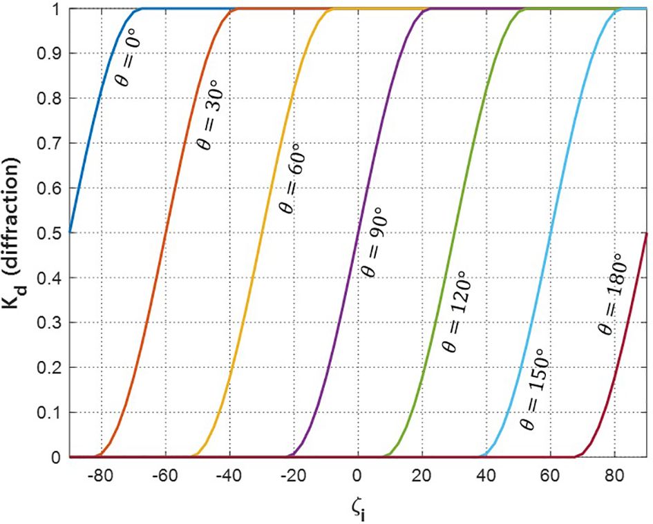
Figure 2 Effects of wave diffraction depending on incident wave direction ($\theta =0°,30°,90°,120°,150°,180°)$.

3.2.2 Wave transmission

Unlike an EDBW that obstructs incoming waves, wave transmission occurs since an SDBW transmits and partially reflects incident wave energy. As shown in Supplementary Figure 4, the initial incident waves may reflect and transmit through the structure. Applying the principle of energy conservation, incident wave energy ($E_i$) equals the sum of three types of wave energy,

$\begin{array}{ll}{\mathit{\text{E}}}_{\mathit{\text{t}}}+{\mathit{\text{E}}}_{\mathit{\text{r}}}+{\mathit{\text{E}}}_{\mathit{\text{dis}}}={\mathit{\text{E}}}_{\mathit{\text{i}}}& (3)\end{array}$

where $E_t$, $E_r$ and $E_{dis}$ represent wave energy due to transmission, reflection, and dissipation, respectively.

From Equation (3), the dimensionless rate of wave energy for transmission, reflection, and dissipation satisfy the relationship (Equation 4),

$\begin{array}{ll}{\mathit{\text{K}}}_{\mathit{\text{t}}}^{\mathbf{2}}+{\mathit{\text{K}}}_{\mathit{\text{r}}}^{\mathbf{2}}+{\mathit{\text{K}}}_{\mathit{\text{dis}}}^{\mathbf{2}}=\mathbf{1}& (4)\end{array}$

where $K_t$ , $K_r$, and $K_{dis}$ denote dimensionless transmission rate, reflection rate, and dissipation rate, respectively, for each wave height ratio concerning the incident wave height (Equations 5a, b). The transmission and reflection coefficients are defined by dividing the transmitted wave height and the reflected wave height by the incident wave height as shown in the following equation.

$\begin{array}{ll}{\mathit{\text{K}}}_{\mathit{\text{t}}}=\frac{{\mathit{\text{H}}}_{\mathit{\text{t}}}}{{\mathit{\text{H}}}_{\mathit{\text{i}}}}& \text{(5a)}\end{array}$

$\begin{array}{ll}{\mathit{\text{K}}}_{\mathit{\text{r}}}=\frac{{\mathit{\text{H}}}_{\mathit{\text{r}}}}{{\mathit{\text{H}}}_{\mathit{\text{i}}}}& \text{(5b)}\end{array}$

where $H_i$, $H_t$ , and $H_r$ represent incident wave height, transmitted wave height, and reflected wave height, respectively.

Laboratory experiments have been conducted to derive the formula for the transmission coefficient over transmissible structures (Takayama et al., 1985; d’Angremond et al., 1996). Joeng et al. (2021) observed the waves in front of and behind the SDBWs at Bongpo-Cheonjin Beach during the passage of typhoon Krosa over the Korean peninsula in 2019. Using the observed wave data, they proposed a formula with an error function to estimate the transmitted wave height over an SDBW. The equation can be expressed simply as follows:

$\begin{array}{ll}{\mathit{\text{H}}}_{\mathit{\text{t}}}=\mathit{\alpha }\mathit{\text{erf}}(\mathit{\text{β}}{\mathit{\text{H}}}_{\mathit{\text{i}}})& (6)\end{array}$

where α and β are coefficients affected by wave breaking and energy dissipation, respectively. And Equation 6 erf is the error function. Therefore, transmission coefficient K_t becomes:

$\begin{array}{ll} {\mathit{\text{K}}}_{\mathit{\text{t}}} =\mathit{\alpha }\mathit{\text{erf}}(\mathit{\text{β}}{\mathit{\text{H}}}_{\mathit{\text{i}}})/{\mathit{\text{H}}}_{\mathit{\text{i}}}& (7)\end{array}$

4 Methodology

This Section proposes a methodology to predict the static equilibrium behind an SDBW. Here, in this paper, static equilibrium is defined as a state in which the longshore sediment rate is in long-term balance. The contents of this section are briefly introduced as follows. Representative studies on longshore sediment rates to calculate static equilibrium are introduced in Subsection 4.1. Subsequently, Subsection 4.2 applies the observed wave climate to predict the static equilibrium of the SDBW in terms of shoreline rotation.

4.1 Longshore sediment transport rate

Longshore sediment transport rate (LSTR) affects shoreline changes. Although there are several different approaches used to quantify the LSTR (CERC, 1984; Kamphuis, 2002; van Rijn, 2002; Bayram et al., 2007; van Rijn, 2014; Lim and Lee, 2023), the empirical relationship between LSTR and energy flux established by Komar and Inman (1970) has been the most popular form. Among these, the CERC (1984) formula using breaking wave condition is given by,

$\begin{array}{ll}{\mathit{\text{Q}}}_{\mathit{\text{l}}}=\frac{\mathit{\text{K}}\sqrt{\mathit{\text{g}}/\mathit{\text{κ}}}}{\mathbf{16}(\mathit{\text{s}}-\mathbf{1})(\mathbf{1}-\mathit{\text{p}})}{\mathit{\text{H}}}_{\mathit{\text{b}}}^{\frac{\mathbf{5}}{\mathbf{2}}}\mathit{\text{sin}}\mathbf{2}{\mathit{\text{α}}}_{\mathit{\text{b}}}=\mathit{\text{C}}\text{'}{\mathit{\text{H}}}_{\mathit{\text{b}}}^{\frac{\mathbf{5}}{\mathbf{2}}}\mathit{\text{sin}}\mathbf{2}{\mathit{\text{α}}}_{\mathit{\text{b}}}& (8)\end{array}$

where $Q_l$ is LSTR, $H_b$ is wave height at the breaking point, and ${\alpha }_b$ is an angle between the breaking wave crest line and the shoreline. The subscript b in Equation (8) refers to wave data at the breaking point, while parameters s, p, $\kappa$, g, and K are specific gravity of beach sand, porosity of beach sand, breaking index, acceleration of gravity, and LSTR coefficient respectively. $C\text{'}$ is a coefficient to represent the characteristics of sand, which has a value of approximately 0.0847. Herein, $s=2.57$, $p=0.35$, $\kappa =0.78$, $g=9.81\text{ m}/s^2$, and $K=0.39$, which are used for most beach sands.

Because most wave data are observed/recorded in deep water rather than at breaking point, deep water wave property is preferred for direct calculation of the LSTR. Assuming depth contours to be straight and parallel to a straight shoreline, Equation (8) can be expressed in deep water wave data (Dean and Dalrymple, 2002), such as,

$\begin{array}{ll}{\mathit{\text{Q}}}_{\mathit{\text{l}},\mathit{\text{O}}}={\mathit{\text{C}}}_{\mathit{\text{O}}}^{\prime }{\mathit{\text{H}}}_{\mathit{\text{O}}}^{\mathbf{2.4}}{\mathit{\text{T}}}_{\mathit{\text{O}}}^{\mathbf{0.2}}\mathbf{\text{cos}}{\mathit{\text{α}}}_{\mathit{\text{O}}}^{\mathbf{1.2}}\mathit{\text{sin}}{\mathit{\text{α}}}_{\mathit{\text{O}}}& (9)\end{array}$

where subscript O represents deep water wave condition. $T_O$ is the wave period at the deep water. ${\mathit{\text{C}}}_O^{\prime }$ is taken approximately 0.0313 for most of the sand under the assumption that the wave direction in the surf zone is negligible. Also, because incident wave direction in deep water varies concerning shoreline direction, the prevailing direction of $Q_{l,O}$ must be adjusted using Equation (10), for the condition that shoreline angle γ (i.e., from N, the north) and incident wave direction ${\theta }_O$, as shown in Supplementary Figure 5,

$\begin{array}{ll}{\mathit{\text{α}}}_{\mathit{\text{O}}}=\frac{\mathit{\text{π}}}{\mathbf{2}}-\mathit{\text{γ}}-{\mathit{\text{θ}}}_{\mathit{\text{O}}}& (10)\end{array}$

Herein, a positive value for LSTR indicates the direction of transport heading southward, while a negative value for heading northward. When a shoreline aligns in a North-South direction and facing eastward, $\gamma =0°$ and waves approaching from the east. On the other hand, when a shoreline facing west, $\gamma =180°$ (clockwise from the N) (Supplementary Figure 5).

For example, with the wave data observed on the central east coast of South Korea, shoreline changes can be estimated using the directional distribution of LSTR by applying Equation (9) (Figure 3). When the predominant wave direction is 42.2° (the shore normal measured clockwise from North), no LSTR occurs (Figure 3). Incoming waves during winter mostly cause the development of southward LSTR, on the other hand, the sediment gets to be transported to the north when the waves flow in during summer (Lim et al., 2022b). If no long-term shoreline changes are found, it is noted that the total northward and southward LSTR balances out, yielding the net LSTR is zero (0). However, if the structure is built, incoming waves get obstructed or transmitted. To maintain the LSTR balance again, the shoreline redistributes, leading to changes in the equilibrium shoreline. Further details on how the shoreline changes behind the SDBW are provided in Section 4.2.

Figure 3

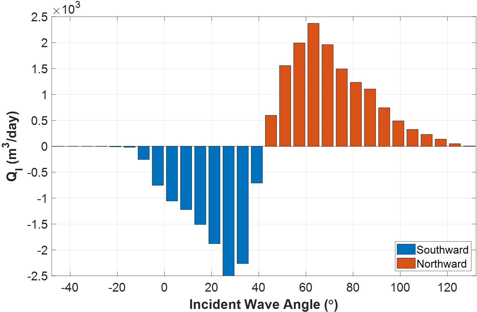
Figure 3 Directional distribution of calculated LSTR on eastern coast of Korea.

4.2 Prediction of static equilibrium behind submerged breakwater

As described in Section 4.1, it is assumed that the shoreline is in equilibrium when the annual average LSTR is zero (0). However, for net LSTR not equal to zero, shoreline change would occur at downdrift or behind SDBW or EDBW, due to wave diffraction and transmission. With the equilibrium shoreline rotating along the curved planform, the value of LSTR can be calculated from wave data for specific locations on the shoreline. The result shown in Figure 4 illustrates the wave rose diagram and the littoral drift diagram, which present the effect of SDBW that causes shoreline rotation. Figure 5 shows wave and shore drift distributions for calculating static equilibrium behind an SDBW ($K_t=0.5$). In Figure 5, the wave distribution represents the $\sum H_O^{2.4}{T}_O^{0.2}$, which is the expression for the wave height and period in Equation (9). Here, wave diffraction is considered at $\theta =120°$ using Equations (2a-c) (see Figure 2). And as shown in the littoral drift distribution in Figure 5, the shoreline rotation angle is calculated so that the sum of the north and south drifts is zero. Therefore, for SDBW with $K_t=0.5$, the shoreline rotation angle is 10.1° when $\theta =120°$.

Figure 4

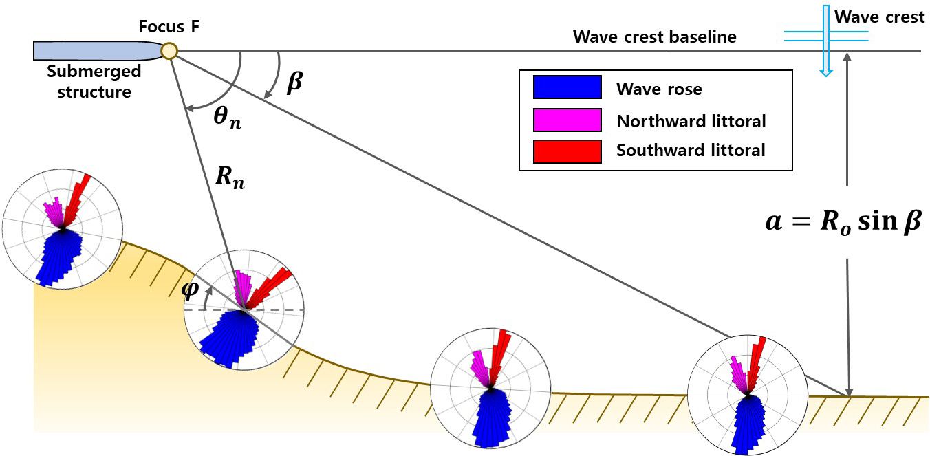
Figure 4 Illustration of static equilibrium behind SDBW using wave and littoral drift roses.

Figure 5

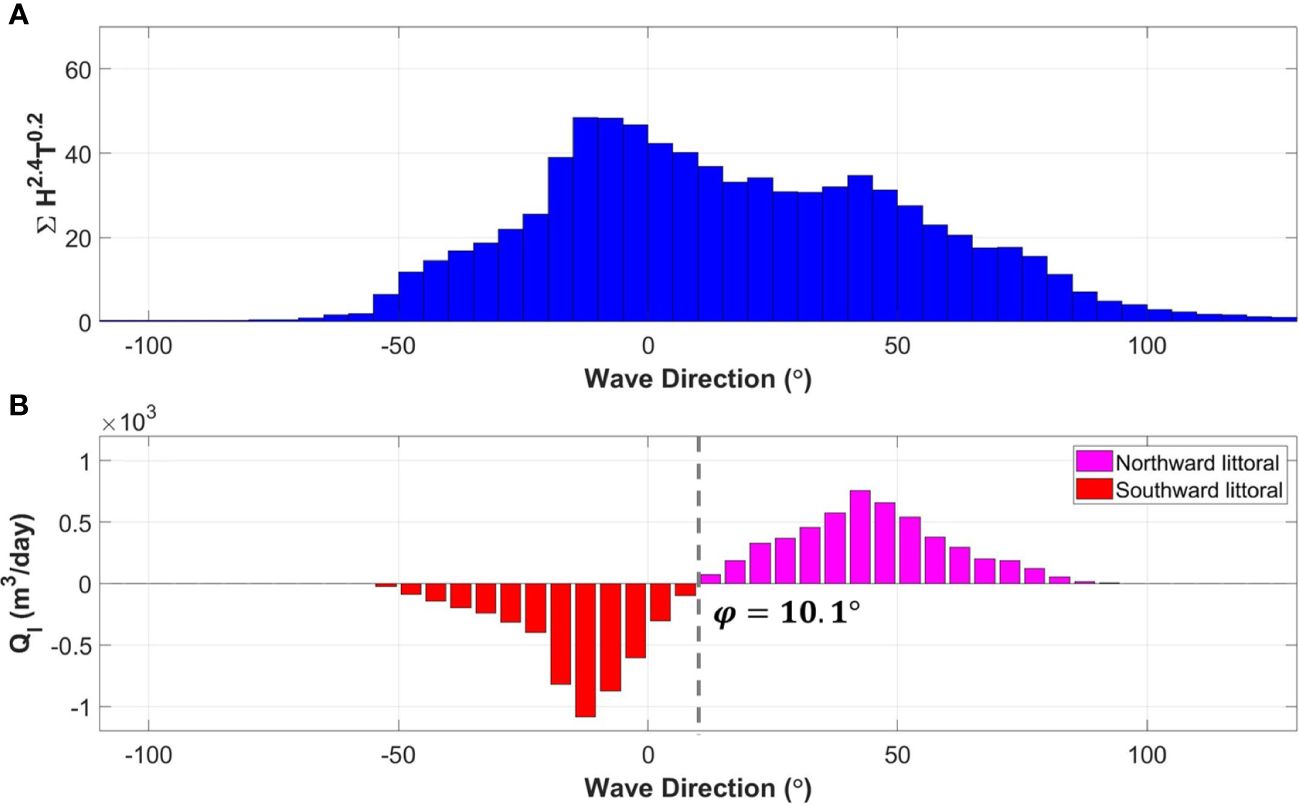
Figure 5 Wave and littoral drift distributions for calculating static equilibrium behind SDBW ($\theta =120°$; $K_t=0.5$): (A) Wave distribution; (B) Littoral drift distribution.

Using wave data introduced in Section 3, the shoreline gradient at which net littoral drift becomes zero is calculated using the CERC formula in Equation (9), reflecting the effect of observed waves being blocked and diffracted by structures, as described above (Lim et al., 2019).

To show the shoreline rotation angles on the eastern coast of Korea (Sec. 2.1), where LSTR is balanced using the CERC formula, the impacts of SDBW on wave deformation can be assessed from wave information (Figure 4). In Figure 6, the red dashed line represents shoreline change resulting from a coastal structure, such as an EDBW, while the blue lines show shoreline rotation angle as a function of transmission coefficient over an SDBW ranging from 0.1 0.9 at an interval of 0.1 (see detail in Supplementary Table 1), depending on the wave setup and tidal conditions.

Figure 6

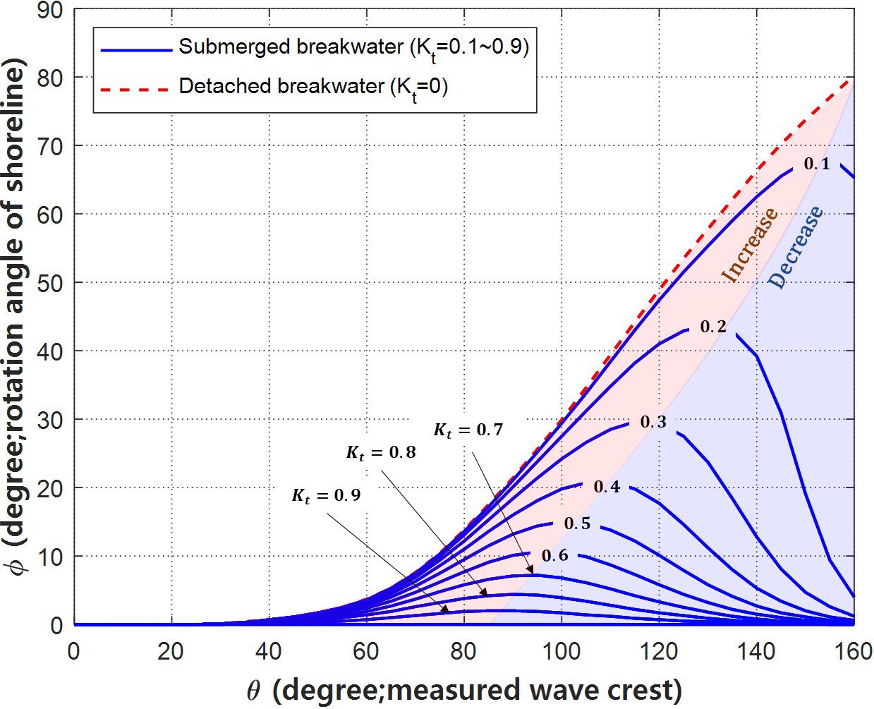
Figure 6 Shoreline rotation angle showing effect of transmission coefficient behind SDBW.

It is necessary to convert the rotation angle to the shoreline. Shoreline rotation angles (φ) can be calculated from a function of the radial distance R, measured from the focus (Figure 4) as follows,

$\begin{array}{ll}{\mathit{\text{R}}}_{\mathit{\text{n}}+\mathbf{1}}={\mathit{\text{R}}}_{\mathit{\text{n}}}\frac{\mathit{\text{sin}}({\mathit{\text{θ}}}_{\mathit{\text{n}}}-\mathit{\text{φ}})}{\mathit{\text{sin}}({\mathit{\text{θ}}}_{\mathit{\text{n}}+\mathbf{1}}-\mathit{\text{φ}})} for {\mathit{\text{θ}}}_{\mathit{\text{n}}}\ge \mathit{\text{β}}& \text{(11a)}\end{array}$

$\begin{array}{ll}{\mathit{\text{R}}}_{\mathit{\text{n}}}=\frac{\mathit{\text{a}}}{\mathit{\text{sin}}{\mathit{\text{θ}}}_{\mathit{\text{n}}}} for {\mathit{\text{θ}}}_{\mathit{\text{n}}}<\mathit{\text{β}}& \text{(11b)}\end{array}$

The static equilibrium shoreline affected by an SDBW can be predicted by applying Equations (11a, b). Thus, prediction of the SEP can be achieved with only the focus point (i.e., diffraction reference point) and the downdrift control point. Figure 7 shows the SEP behind an SDBW (100 m in length and at 50 m offshore) with transmission coefficients of 0.2, 0.4, 0.6, and 0.8, respectively. Here, the static equilibrium was calculated from the rotation angle depending on the transmission coefficient, respectively, shown in Supplementary Table 1. In addition, Figure 8 shows the SEP behind three SDBWs (100 m in length and at 50 m offshore and 200 m gap) with transmission coefficients of 0.2, 0.4, 0.6, and 0.8, respectively. The hinterland shoreline gradient caused by each detached breakwater is calculated independently. However, if the surrounding breakwater is within the affected area, Equations (11a, b) are applied in proportion to the distance so that the hinterland shoreline gradient is determined. Therefore, the governing equation of this model, derived from continuous equations, allows it to preserve the entire beach surface area and naturally predict shoreline changes behind multiple coastal structures.

Figure 7

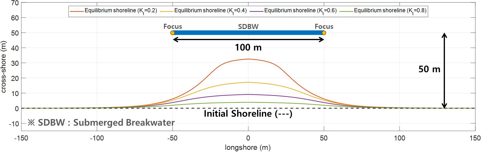
Figure 7 Static equilibrium shoreline behind SDBW with various transmission coefficients ($K_t=0.2,0.4,0.6$ and 0.8).

Figure 8

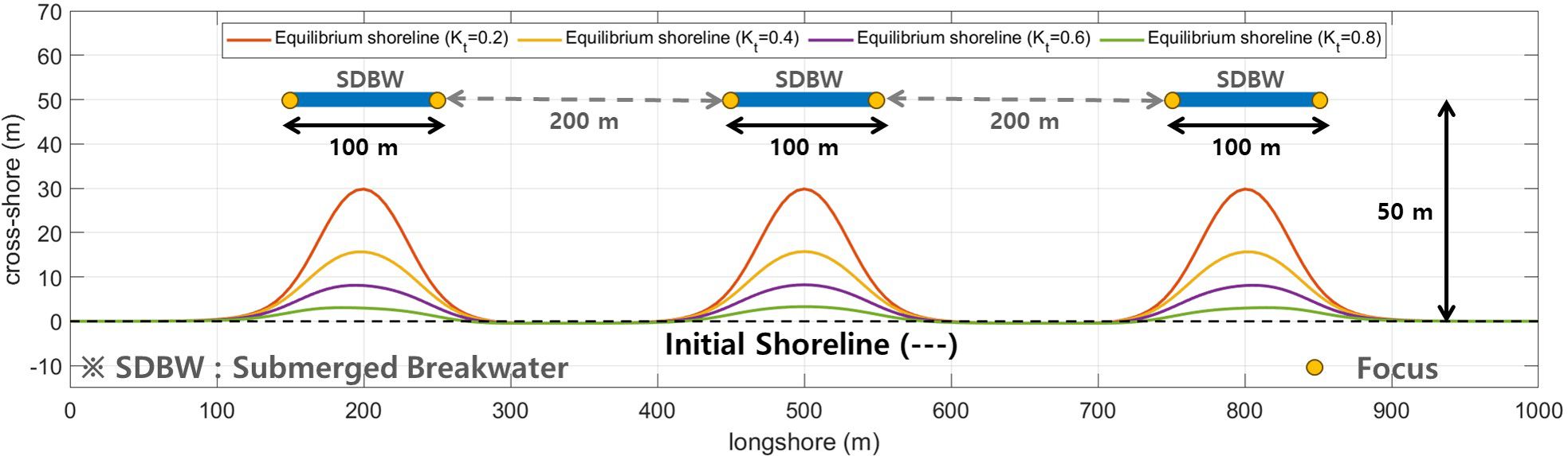
Figure 8 Static equilibrium shoreline behind three SDBWs with various transmission coefficients ($K_t=0.2,0.4,0.6$ and 0.8).

5 Results

The methodology presented in this study is applied to predict shoreline changes due to the construction of SDBW on the east coast of South Korea and the results are compared with that from field observation. The impacts of shoreline changes resulting from the construction of single and multiple structures are different. Therefore, the study sites applied to this section are Anmok Beach (37°46’N, 128°57’E), which has a single SDBW, and Bongpo-Cheonjin Beach (38°15’N, 128°33’E), which has three SDBWs.

5.1 Single SDBW - Anmok Beach

5.1.1 Study site description

Anmok Beach is a straight coast that extends long to the north from Gangneung Harbor (Figure 9). The average grain size of the sand at Anmok Beach is 0.4 mm. Anmok Beach has a shoreline orientation of N48.4°E, extending from northwest to southeast. Anmok Beach suffered continuous erosion damage after the construction of Gangneung Port in 1991 as littoral cells separated from Namdae-cheon (river), the source of sedimentation. Therefore, the Ministry of Oceans and Fisheries in Korea constructed an SDBW (252 m) and one submerged groin (100 m) to reduce beach erosion. Additionally, beach nourishment was conducted on approximately 20,129 m². After the construction of the SDBW was completed, waves were observed before and after the structure to analyze the transmission coefficient. Supplementary Figure 6 shows the observed transmission coefficient compared to the results of the error function of Equation (7). Here, the coefficients α and β are 0.65 and 1.35, respectively.

Figure 9

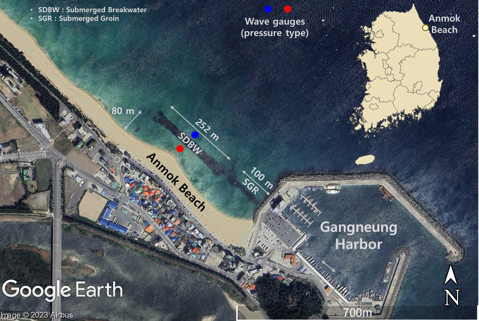
Figure 9 Location of Anmok Beach and wave gauges to observe incident and transmitted waves of SDBW (^© Google Earth).

5.1.2 Verification of predicted shoreline

As previously mentioned, this subsection predicts the equilibrium shoreline after a single SDBW is constructed. Therefore, this subsection predicts the equilibrium shoreline when only one structure is built at Anmok Beach. The shoreline in July 2015, when only one SDBW was built, was extracted from aerial photographs. At the time of shoreline extraction, the beach was assumed to be the static equilibrium. As shown in Figure 10, the shoreline observed from Anmok Beach clearly has the salient behind the SDBW. And the equilibrium shoreline was predicted using the annual mean wave because the waves were calm during July 2015. Supplementary Figure 7 shows the temporal series of breaking waves observed at Anmok Beach from September 17, 2014, to September 16, 2015 (37°53’N, 129°10’E). Here, breaking wave height was calculated assuming the water depth contours were straight and parallel to the shoreline. According to the wave data observed at Anmok Beach from September 17, 2014, to September 16, 2015, the mean wave height, period, and direction are 1.15 m, 7.65 sec, and 49.8°, respectively. Therefore, the transmission coefficient of the SDBW at Anmok Beach is calculated to be 0.55 when the mean wave height is 1.15 m as shown in Supplementary Figure 6.

Figure 10

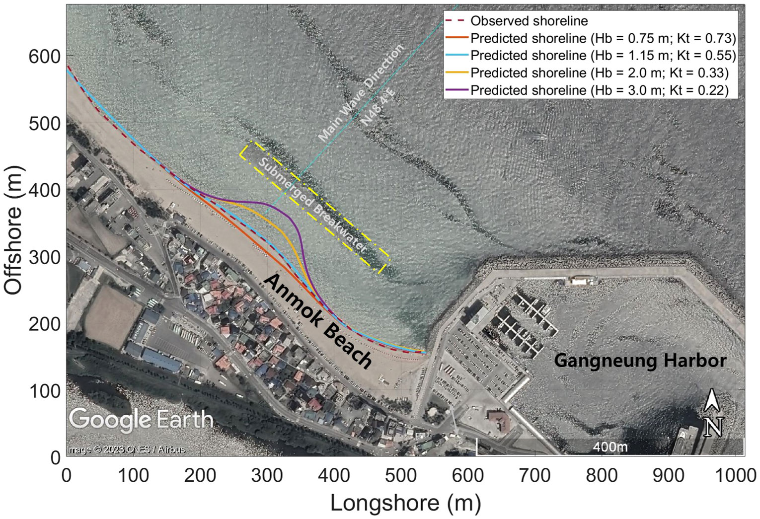
Figure 10 Comparison of shoreline extracted from aerial image and that predicted by methodology in this study (^© Google Earth).

According to the aerial image in Figure 10, deposition occurred in the southern area of Anmok Beach owing to the construction of Gangneung Harbor. Therefore, the equilibrium shoreline from Gangneung Harbor to the north owing to the harbor was predicted using PBSE, which predicts the SEP owing to EDBW (Section 2). Figure 10 compares the shoreline extracted from the aerial image with that predicted using the methodology proposed in this study. Here, the transmission coefficient for the annual mean wave was assumed to be constant at 0.55. It also shows the calculated SEP planform is in good agreement with the observed, and the deposition width of the salient, is also similar to the observed. Figure 10 also shows transmission coefficient ($K_t=0.73 \text{for} H_b=0.75\text{ m}$, $K_t=0.55 \text{for} H_b=1.15\text{ m}$, $K_t=0.33 \text{for} H_b=2.0\text{ m}$and $K_t=0.22 \text{for} H_b=3.0\text{ m}$) influence the salient formation owing to the SDBW construction.

5.2 Multiple SDBWs - Bongpo-Cheonjin Beach

5.2.1 Study site description

Bongpo-Cheonjin Beach is approximately 1.1 km long, with a crenulated-shaped bay between two harbors; Cheonjin Harbor in the northern and Bongpo Harbor in the southern, respectively (Figure 11). The representative grain size of the sand within the limit of littoral movement is 0.62 mm. Bongpo-Cheonjin Beach has a shoreline orientation of N53.4°E, extending from northwest to southeast. The Ministry of Oceans and Fisheries in Korea started an improvement project in which four SDBWs (490 m in total) and one groin (GR; 40 m long) were constructed (Figure 11) to mitigate erosion. The construction project commenced in 2017 and completed in November 2019. Afterward, wave observations were conducted before and after the structure to verify the performance of SDBW. Supplementary Figure 8 shows the observed transmission coefficient compared to the results of the error function of Equation (7). Here, the coefficients α and β are 0.98 and 0.80, respectively.

Figure 11

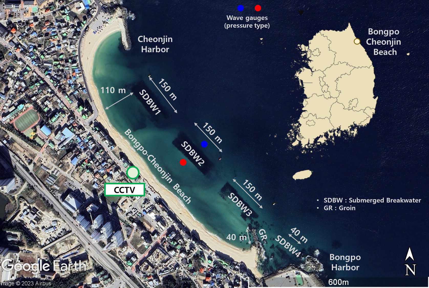
Figure 11 Location of Bongpo-Cheonjin Beach and wave gauges to observe incident and transmitted waves of SDBW (^© Google Earth).

5.2.2 Verification of predicted shoreline

Bongpo-Cheonjin Beach has been covered by four closed-circuit televisions (CCTV) from May 2015 to the present (Figure 11), in which the coordinates on the video reference points have been set for extracting the shoreline information from CCTV images. From beach images, salient shapes during relatively high waves are extracted to verify the methodology presented in this paper. This is carried out by applying the wave data provided by the Korea Meteorological Administration, for high waves occurring on Bongpo-Cheonjin Beach from December 8, 2020, to January 7, 2021 (38°22’N, 128°32’E). Supplementary Figure 9 shows the breaking waves over that period. Here, breaking waves are calculated from wave data observed in deep water based on wave shoaling and refraction. The mean wave height, period and direction are 1.09 m, 7.42 sec, and 50.8°, respectively. According to Equation (7), the transmission coefficient of the SDBW at Bongpo-Cheonjin Beach is calculated to be 0.70 when the mean wave height is 1.09 m.

According to the CCTV image in Figure 12, the central salient is biased toward the south because the average wave direction and shoreline orientation differ by approximately 2.6°. Therefore, this difference was reflected in Equationd (11a, b) to predict the equilibrium shoreline. The SEP owing to two harbors was predicted using PBSE introduced in Section 2. Figure 12 compares the shoreline planform extracted from CCTV images with that predicted using the approach presented in this study. Here, the transmission coefficient of three SDBWs was assumed to be constant at 0.7. The overall extent of deposition and erosion is similar when comparing observed and predicted shorelines. However, the overall patterns are slightly different. This different pattern is presumed to be caused by longshore currents owing to the diverse coastal structures built at Bongpo-Cheonjin Beach.

Figure 12

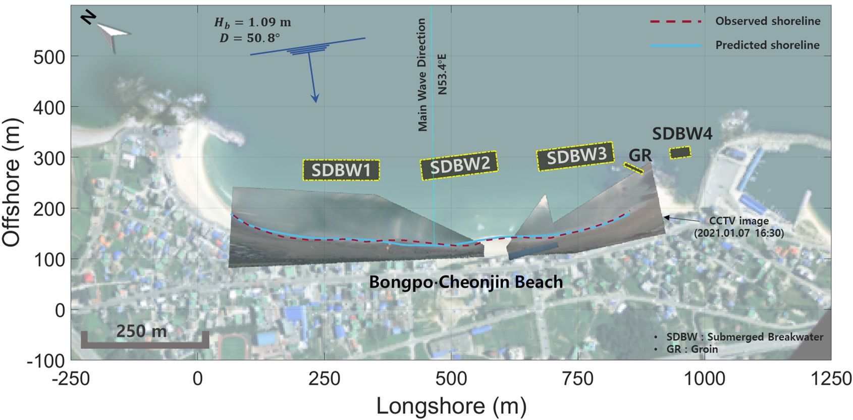
Figure 12 Comparison of shoreline extracted from CCTV image and that predicted by methodology in this study. Adapted with permission from Evaluation of beach response due to construction of submerged detached breakwater by Changbin Lim, Jinhoon Kim, Jong-Beom Kim and Jung-Lyul Lee, licensed under CC-BY-4.0, National Geographic Information Institute (NGII), Republic of Korea.

6 Discussions

Subsection 6.1 discusses to limitations of the methodology presented in this study. Subsection 6.2 discusses to which wave environments the methodology of this paper can be applied in terms of wave direction distribution. Additionally, the methodology of this paper is applied to the extreme conditions in Subsection 6.3. Lastly, Subsection 6.4 discusses the application of this paper’s methodology to temporal shoreline changes.

6.1 Limitations

In this section, additional considerations and limits for a research methodology will be briefly described. First, difficulties exist in the accurate prediction of wave deformation caused by the presence of submerged transmissible coastal structures, such as submerged DBWs (SDBWs) consisting of precast concrete blocks. Thus, the SEP in the vicinity of these structures should be considered as an estimate using the relatively simple equation for wave diffraction and transmission. In this process, the wave transmission coefficient and reflection coefficient are calculated assuming that there is no wave energy loss. Therefore, it is necessary to consider accurate wave energy dissipation and wave diffraction through hydraulic experiments before constructing SDBWs.

In addition, years of wave observation data from the East Sea, South Korea, was used to predict shoreline changes behind the SDBW. The selected study area does not have characteristics representative of all beaches because its seasonal wave environments are seen with distinctively different patterns. Thus, it is necessary to apply the mechanism estimated by this research to different beaches and verify its usability. In Section 6.2, static equilibrium shorelines are predicted based on the wave directional distribution to enhance the applicability of the methodology in this paper.

Lastly, how each structure affects the SEP was estimated and shoreline changes were predicted from the optimal calculation results. However, depending on a gap or a distance in multi-arrayed SDBWs, the same effect can be seen as the impact that a single large-sized SDBW has on shoreline changes. Thus, additional in-depth research on estimating how multi-arrayed SDBWs affect the SEP is needed.

6.2 Wave directional distribution in East Sea of South Korea

The methodology in this paper directly used the globally recognized CERC (1984) formula to calculate LSTR. Unlike other formulas, the CERC (1984) formula does not take into account the grain size of the sand. Therefore, the most important thing to estimate the SEP behind the SDBW is the wave climate. Subsection 6.2 describes the directional distribution of the long-term wave observations used in this paper. In addition, this subsection compares the result with a representative function for the directional spectrum. Mitsuyasu and Mizuno (1976) extracted directional spectra from multi-year wave data observed in Japan and proposed the directional distribution function Equation 12 as follows:

$\begin{array}{ll}\mathit{\text{D}}(\mathit{\text{θ}})=\frac{{\mathbf{2}}^{\mathbf{2}\mathit{\text{s}}}}{\mathbf{2}\mathit{\text{π}}}\frac{{\mathit{\text{Γ}}}^{\mathbf{2}}(\mathit{\text{S}}+\mathbf{1})}{\mathit{\text{Γ}}(\mathbf{2}\mathit{\text{S}}+\mathbf{1})}{\mathit{\text{cos}}}^{\mathbf{2}\mathit{\text{s}}}(\mathit{\text{θ}}/\mathbf{2})& (12)\end{array}$

where Γ is the gamma function and s is the spreading parameter.

Using the observed wave data (see Section 3), the wave directional distribution is calculated as shown in Supplementary Figure 10. Compared to the wave direction distribution function proposed by Mitsuyasu and Mizuno (1976), the eastern series (0° ~ 90°), which shows a relatively gentle distribution, has S = 8.2. On the other hand, the northern series (-90° ~ 0°), which shows a relatively sharp distribution, has S = 19.7. The results of this paper apply to wave climates with similar directional distributions (S = 8.2 for the eastern series; S = 19.7 for the northern series).

Furthermore, the methodology in this paper can be applied even if only the directional distribution is known, rather than the long-term observed wave data. Figure 13 shows the shoreline rotation angles when the spreading parameters are 8, 12, 20, and 36, respectively. In Figure 13, the smaller the spreading parameter, the larger the peak rotation angle and the more it is biased toward the center of the structure. Supplementary Figure 11 shows the SEP behind an SDBW (100 m in length and at 50 m offshore; $K_t=0.5$) with spreading parameters of 8, 12, 20, and 36, respectively. Supplementary Figure 11 shows how spreading parameters influence the salient formation owing to the SDBW construction.

Figure 13

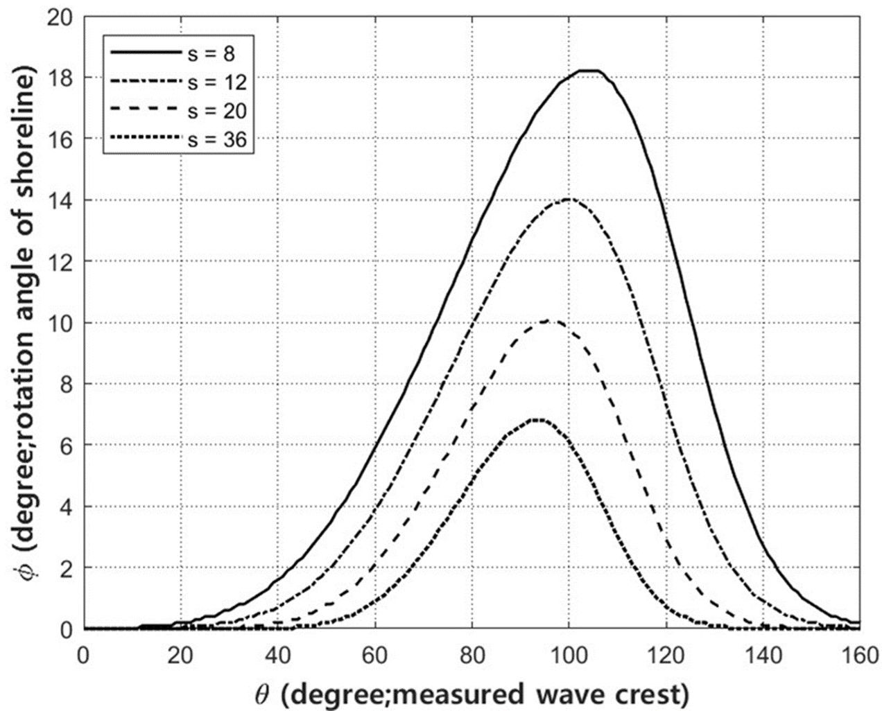
Figure 13 Shoreline rotation angle behind SDBW ($K_t=0.5$) according to directional distributions ($s=8,12,20\text{ and }36$).

6.3 Estimation of shoreline retreat for specific return period

The primary purpose of building an SDBW is to reduce damage from storm waves. While this paper has primarily focused on predicting the SEP behind an SDBW, this subsection extends that to predicting shoreline retreat for a specific return period. In Gangwon-do, Korea, a minimum of 4 times annual shoreline observations have been conducted to analyze the seasonal change since 2010. Lim et al. (2021b) analyzed a normal distribution utilizing the shoreline data of Bongpo-Cheonjin Beach observed for a total of 37 times for 10 years from 2008 to 2017. Supplementary Figure 12 shows a comparison of the observed shoreline histogram and a normal distribution equation. Herein, the standard deviation σ of the shoreline variation width data is 5.5 m. Lim et al. (2021b) statistically calculated the eroded shoreline for a specific return period. In this subsection, the methodology of this paper applies a shoreline retreat of 19.75 m, which is a 30-year return period for Bongpo-Cheonjin Beach. Shoreline retreat behind the four SDBWs can be predicted using the methodology presented in this paper. Joeng et al. (2021) reported that the 30-year return period wave height at Bongpo-Cheonjin Beach is approximately 6.48 m. And transmission coefficient is calculated to be 0.15 when the waves hit in a 30-year period. The eroded shorelines were estimated by setting control points from the location in which about 19.75 m was moved backward from the initial ones. Therefore, static equilibrium is predicted when the transmission coefficient is 0.15 at the retreated control point. This occurred on a narrow stretch between SDBW1 and SDBW2 as indicated in Figure 14.

Figure 14

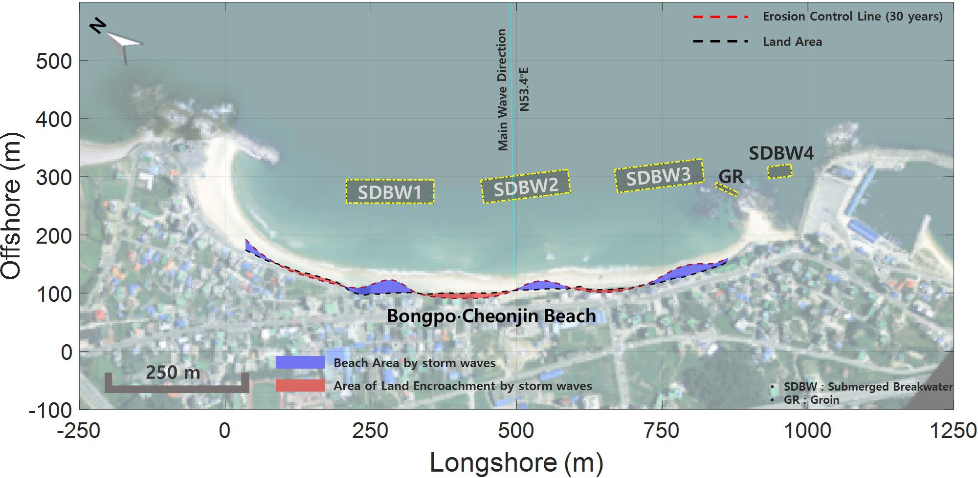
Figure 14 Shoreline retreat due to storm waves with 30-year return period. Adapted with permission from Evaluation of beach response due to construction of submerged detached breakwater by Changbin Lim, Jinhoon Kim, Jong-Beom Kim and Jung-Lyul Lee, licensed under CC-BY-4.0, National Geographic Information Institute (NGII), Republic of Korea.

6.4 Estimation of equilibrium shoreline change

A one-line shoreline change model incorporating shoreline rotation in the wave diffraction zone is used to simulate behind an SDBW with a specific transmission coefficient. The governing equation was originally proposed by Pelnard-Considère (1957) for a system of short groins without wave diffraction to determine shoreline positions based on LSTR differences. The model assumes erosion and deposition within an active volume measured from the berm to the depth of closure is constant (Equation 13).

$\begin{array}{ll}\frac{\mathit{\partial }\mathit{\text{x}}}{\mathit{\partial }\mathit{\text{t}}}+\frac{\mathbf{1}}{({\mathit{\text{h}}}_{\mathit{\text{c}}}+{\mathit{\text{h}}}_{\mathit{\text{B}}})}\frac{\mathit{\partial }{\mathit{\text{Q}}}_{\mathit{\text{l}}}}{\mathit{\partial }\mathit{\text{y}}}=\mathbf{0}& (13)\end{array}$

where $h_c$ is the depth of closure and $h_B$ is the berm height. the value of each LSTR $Q_l$ can be estimated using the CERC formula (CERC, 1984). Shoreline position is represented by Cartesian coordinate in which x is measured in the cross-shore direction, while yy is in the alongshore direction.

The value of $Q_l$ can be calculate by deep water wave data, as in Equation (9), but with modified wave angle ${\alpha }_m$ along the rotated SEP calculated by the PBSE, instead of ${\alpha }_0$, in Equation (14),

$\begin{array}{ll}{\mathit{\text{Q}}}_{\mathit{\text{l}},\mathit{\text{O}}}={\mathit{\text{C}}}_{\mathit{\text{O}}}^{\prime }{\mathit{\text{H}}}_{\mathit{\text{O}}}^{\mathbf{2.4}}{\mathit{\text{T}}}_{\mathit{\text{O}}}^{\mathbf{0.2}}\mathit{\text{cos}}{\mathit{\alpha }}_{\mathit{\text{m}}}^{\mathbf{1.2}}\mathit{\text{sin}}{\mathit{\text{α}}}_{\mathit{\text{m}}}& (14)\end{array}$

where ${\alpha }_m$refers to an angle of diffracted waves within the shadow zone of a SDBW (Lim et al., 2021a) and wave transmission coefficient per Figure 6.

SEP behind the SDBWs at Bongpo-Cheonjin Beach is calculated using transmission coefficient K_t = 0.70 over the submerged structures. The results of the numerical calculation are depicted in Figure 15 for shoreline changes after the construction of SDBWs on Bongpo-Cheonjin Beach, shoreline changes for 1 month, 3 months, and 1 year, respectively, assuming active vertical depth 7.0 m with wave transmission coefficient for normal waves as 0.70. Here, the mean wave height, period, and direction are applied to be 1.09 m, 7.42 sec, and 50.8°, respectively. Upon comparing the calculated results with the shoreline on the existing aerial photograph, no noticeable shoreline changes have occurred in the north part of the beach, while minor deposition is behind SDBW1 which was constructed last. A small salient SDBW2 was constructed in the center of the beach, the salient was formed at the sagged point of the shoreline behind the structure, which is located on the southern side from the center. Lastly, because SDBW3 and the groin were built closely to each other, they work collectively as a long groin, resulting in shoreline advancement in the south part of the beach.

Figure 15

Figure 15 Simulation of shoreline change model due to construction of SDBWs ($K_t=0.70$) and GR ($K_t=0.70$) in Bongpo-Cheonjin Beach: (A) Overview; (B) Zone 1; (C) Zone 2; (D) Zone 3; (E) Zone 4. Adapted with permission from Evaluation of beach response due to construction of submerged detached breakwater by Changbin Lim, Jinhoon Kim, Jong-Beom Kim and Jung-Lyul Lee, licensed under CC-BY-4.0, National Geographic Information Institute (NGII), Republic of Korea.

7 Conclusion

This study presents a methodology to estimate the shoreline change behind an SDBW constructed on an embayed beach on the east coast of South Korea. Utilizing observed wave data sets, the research aims to provide a method of measuring the rotation angle of the equilibrium shoreline. The summary is as follows. Firstly, impacts of structures on diffracted waves are also included, secondly, transmission rates affected by SDBW are reflected in observed wave data. Lastly, the shoreline angle is determined when LSTR is balanced (0), using the CERC formula that is applied to open sea waves. Here, the LSTR is calculated from the CERC equation under deep water conditions using observed waves in deep water. SDBW has characteristics of not completely obstructing incident waves, i.e. partially reflecting yet transmitting to a certain degree. Because of this, it is found that shoreline rotation angles behind the SDBW tend to increase and then decrease, unlike the SDBW. The computed angle is used here to predict a change in the equilibrium shoreline. As depicted above, the shoreline rotation angles can be calculated from a function of the radius distance R, which was measured at an angle θ from the focus.

The proposed model simulates how the equilibrium shoreline changes based on the rotation angle results from the impacts of the SDBW. This methodology shows satisfactory results by applying it to two beaches located on the east coast of Korea. Accurate predictions of shoreline changes are very important in that instead of benefits that can be caused by submerged breakwaters (i.e., reduction of beach erosion), they bring about opposite effects; sand will accumulate toward a breakwater, thus further causing beach erosion. Therefore, the results derived from this study, on predicting how a shoreline may change after installing a series of SDBWs, will benefit the technical designers and coastal managers. In addition, this methodology can be extended to predict shoreline changes due to storm waves. However, further studies on shoreline changes occurring behind submerged breakwaters should be conducted in more diverse settings where dynamic responses of wave actions can be investigated.

Data availability statement

The raw data supporting the conclusions of this article will be made available by the authors, without undue reservation.

Author contributions

CL: Writing – original draft, Writing – review & editing, Visualization, Methodology, Data curation, Conceptualization. JK: Writing – review & editing, Data curation. J-BK: Writing – review & editing, Data curation. J-LL: Writing – review & editing, Supervision, Methodology, Conceptualization.

Funding

The author(s) declare that financial support was received for the research, authorship, and/or publication of this article. This research was supported by the Korea Institute of Marine Science & Technology Promotion (KIMST), funded by the Ministry of Oceans and Fisheries, Korea (RS-2023-00256687).

Conflict of interest

Author J-BK is employed by GeoSystem Research Corporation.

The remaining authors declare that the research was conducted in the absence of any commercial or financial relationships that could be construed as a potential conflict of interest.

Publisher’s note

All claims expressed in this article are solely those of the authors and do not necessarily represent those of their affiliated organizations, or those of the publisher, the editors and the reviewers. Any product that may be evaluated in this article, or claim that may be made by its manufacturer, is not guaranteed or endorsed by the publisher.

Supplementary material

The Supplementary Material for this article can be found online at: https://www.frontiersin.org/articles/10.3389/fmars.2024.1367411/full#supplementary-material

Supplementary Figure 1 | Definition sketch of parabolic bay shape equation.

Supplementary Figure 2 | Location of acoustic wave and current meter (AWAC) to observe wave climate on eastern coast of Korea (© Google Earth).

Supplementary Figure 3 | Temporal series of wave data observed on eastern coast of South Korea: (A) significant wave height; (B) peak wave period; (C) significant wave direction.

Supplementary Figure 4 | Definition sketch of reflection and transmission of waves induced by SDBW.

Supplementary Figure 5 | Direction of LSTR according to incident wave direction and shoreline from true north (reproduced from Lim et al., 2022b, licensed CC-BY-4.0).

Supplementary Figure 6 | Analysis of incident wave height and transmission coefficient for SDBW on Anmok Beach.

Supplementary Figure 7 | Temporal series of breaking waves at Anmok Beach from September 17, 2014, to September 16, 2015.

Supplementary Figure 8 | Analysis of incident wave height and transmission coefficient for SDBW on Bongpo-Cheonjin Beach.

Supplementary Figure 9 | Temporal series of breaking waves at Bongpo-Cheonjin Beach from December 8, 2020, to January 7, 2021.

Supplementary Figure 10 | Comparison of wave directional distribution on eastern coast of Korea and directional distribution function (Equation 12).

Supplementary Figure 11 | Static equilibrium shoreline behind SDBW ($K_t=0.5$) according to directional distributions ($s=8,12,20\text{ and }36$).

Supplementary Figure 12 | Comparison between shoreline observation data of Bongpo-Cheonjin Beach in South Korea and normal distribution equation.

Supplementary Table 1 | Shoreline rotation angle according to wave transmission rate K_t and radial angle measured from wave θ.

References

Ahrens J. P., Cox J. (1990). Design and performance of reef breakwaters. J. Coast. Res. 1, 61–75. Available at: https://www.jstor.org/stable/25735389

Google Scholar

Bayram A., Larson M., Hanson H. (2007). A new formula for the total longshore sediment transport rate. Coast. Eng. 54, 700–710. doi: 10.1016/j.coastaleng.2007.04.001

CrossRef Full Text | Google Scholar

CERC (1984). “Shore protection manual,” in U.S. Army Corps of Engineers, Waterways Experiment Station, Coastal Engineering Research Center, U.S, 4th Ed (Government Printing Office, Washington, D.C).

Google Scholar

Dally W. R., Pope J. (1986). Detached breakwaters for shore protection. Technical Report CERC-86-1 (Vicksburg, MS: U.S. Army Engineer Waterways Experiment Station). doi: 10.5962/bhl.title.48331

CrossRef Full Text | Google Scholar

Davidson M. A., Splinter K. D., Turner I. L. (2013). A simple equilibrium model for predicting shoreline change. Coast. Eng. 73, 191–202. doi: 10.1016/j.coastaleng.2012.11.002

CrossRef Full Text | Google Scholar

d’Angremond K., van der Meer J. W., De Jong R. J. (1996). “Wave transmission at low-crested structures,” in Proc. 25th Inter. Conf. on Coastal Engineering. ASCE, 3305–3318. doi: 10.1061/9780784402429.187

CrossRef Full Text | Google Scholar

Dean R., Dalrymple R. (2002). Coastal Processes with Engineering Applications (Cambridge: Cambridge University Press, Cambridge, UK), 475. doi: 10.1017/CBO9780511754500

CrossRef Full Text | Google Scholar

Elshinnawy A. I., Medina R., González M. (2018). On the influence of wave directional spreading on the equilibrium planform of embayed beaches. Coast. Eng. 133, 59–75. doi: 10.1016/j.coastaleng.2017.12.009

CrossRef Full Text | Google Scholar

Elshinnawy A. I., Medina R., González M. (2022). Equilibrium planform of pocket beaches behind breakwater gaps: on the location of the intersection point. Coast. Eng. 173, 104096. doi: 10.1016/j.coastaleng.2022.104096

CrossRef Full Text | Google Scholar

González M., Medina R. (2001). On the application of static equilibrium bay formulations to natural and man-made beaches. Coast. Eng. 43, 209–225. doi: 10.1016/S0378-3839(01)00014-X

CrossRef Full Text | Google Scholar

González M., Medina R., Losada M. A. (2010). On the design of beach nourishment projects using static equilibrium concepts: Application to Spanish coast. Coast. Eng. 57(2), 227–240. doi: 10.1016/j.coastaleng.2009.10.009

CrossRef Full Text | Google Scholar

Gourlay M. R. (1981). “Beach processes in the vicinity of offshore breakwaters,” in Proc. Fifth Australian Conference on Coastal and Ocean Engineering. Australian National Conference Publications, 129–134.

Google Scholar

Hanson H., Kraus N. C. (1989). Genesis: Generalized Model for Simulating Shoreline Change, Report 1: Reference Manual and Users Guide. Technical Report CERC-89-19, U.S. Army Engineer Waterways Experiment Station, Coastal Engineering Research Center, Vicksburg MS.

Google Scholar

Herbich J. B. (1989). “Shoreline change due to offshore breakwaters.” Proc. 23rd International Association for Hydraulic Research Congress, Ottawa, Canada, C317–C327.

Google Scholar

Hsu J. R. C., Evans C. (1989). Parabolic bay shapes and applications. Proc. Inst. Civil Engineers Part 2 87, 557–5570. doi: 10.1680/iicep.1989.3778

CrossRef Full Text | Google Scholar

Hsu J. R. C., Silvester R. (1990). Accretion behind single offshore breakwater. J. Waterway Port Coast. Ocean Eng. 116, 362–381. doi: 10.1061/(ASCE)0733-950X(1990)116:3(362)

CrossRef Full Text | Google Scholar

Hur D. S. (2004). Deformation of multi-directional random waves passing over an impermeable submerged breakwater installed on a sloping bed. Ocean Eng. 31, 1295–1311. doi: 10.1016/j.oceaneng.2003.12.005

CrossRef Full Text | Google Scholar

Inman D. L., Frautschy J. D. (1965). “Littoral processes and the development of shoreline.“ Proc. Santa Barbara Specialty Conf. Costal Eng. ASCE, New York, NY, 511–536.

Google Scholar

Jara M. S., González M., Medina R. (2015). Shoreline evolution model from a dynamic equilibrium beach profile. Coast. Eng. 99, 1–14. doi: 10.1016/j.coastaleng.2015.02.006

CrossRef Full Text | Google Scholar

Jaramillo C., Jara M. S., González M., Medina R. (2020). A shoreline evolution model considering the temporal variability of the beach profile sediment volume (sediment gain / loss). Coast. Eng. 156, 103612. doi: 10.1016/j.coastaleng.2019.103612

CrossRef Full Text | Google Scholar

Jaramillo C., Jara M. S., González M., Medina R. (2021). A shoreline evolution model for embayed beaches based on cross-shore, planform and rotation equilibrium models. Coast. Eng. 169, 103983. doi: 10.1016/j.coastaleng.2021.103983

CrossRef Full Text | Google Scholar

Joeng J.-H., Kim J. H., Lee J.-L. (2021). Analysis of wave transmission characteristics on the TTP submerged breakwater using a parabolic-type linear wave deformation model. J. Ocean Eng. Technol. 35, 82–90. doi: 10.26748/KSOE.2020.066

CrossRef Full Text | Google Scholar

Kamphuis J. W. (2002). “Alongshore transport of sand,” in Proc. 28th Int. Conf. Coastal Eng. (Cardiff, Wales: ASCE), 2478–2490, Cardiff, Wales, 7 – 12 July. doi: 10.1142/5165

CrossRef Full Text | Google Scholar

Kang Y. K., Park H. B., Yoon H. S. (2010). Shoreline changes caused by the construction of coastal erosion control structure at the Youngrang Coast in Sokcho, East Korea. J. Korean Soc. Mar. Environ. Eng. 13, 296–304.

Google Scholar

Kim T.-K., Lee J.-L. (2018). Analysis of shoreline response due to wave energy incidence using equilibrium beach profile concept. J. Ocean Eng. Technol. 32, 116–122. doi: 10.26748/KSOE.2018.4.32.2.116

CrossRef Full Text | Google Scholar

Kim T. K., Lim C., Lee J. L. (2021). Vulnerability analysis of episodic beach erosion by applying storm wave scenarios to a shoreline response model. Front. Mar. Sci. 8, 759067. doi: 10.3389/fmars.2021.759067

CrossRef Full Text | Google Scholar

Kobayashi N., Wurjanto A. (1989). Wave overtopping on coastal structures. J. Waterway Port Coastal Ocean Eng. 115, 235–251. doi: 10.1061/(ASCE)0733-950X(1989)115:2(235)

CrossRef Full Text | Google Scholar

Komar P. D., Inman D. L. (1970). Longshore and transport on beaches. J. Geophys. Res. 75(30), 5914–5927. doi: 10.1029/JC075i030p05914

CrossRef Full Text | Google Scholar

Lausman R., Klein A. H. F., Stive M. J. F. (2010a). Uncertainty in the application of parabolic bay shape equation: Part 1. Coast. Eng. 57, 132–141. doi: 10.1016/j.coastaleng.2009.09.009

CrossRef Full Text | Google Scholar

Lausman R., Klein A. H. F., Stive M. J. F. (2010b). An uncertainty in the application of parabolic bay shape equation: Part 2. Coast. Eng. 57, 142–151. doi: 10.1016/j.coastaleng.2009.10.001

CrossRef Full Text | Google Scholar

Lee W. D., Her D. S., Park J. B., An S. W. (2009). A study on effect of beachface gradient on 3-D currents around the open inlet of submerged breakwaters. J. Ocean Eng. Technol. 23(1), 7–15.

Google Scholar

Lee J. L., Lim C., Pranzini E., Yu M. J., Chu J. C., Chen C. J., et al. (2023). Assessing common downdrift control point and asymmetric double-curvature planform behind multiple detached breakwaters: Simple empirical method. Coast. Eng. 185, 104361. doi: 10.1016/j.coastaleng.2023.104361

CrossRef Full Text | Google Scholar

Lim C., Hsu J. R. C., Lee J. L. (2022a). MeePaSoL: A MATLAB-based GUI software tool for shoreline management. Comput. Geosciences 161, 105059. doi: 10.1016/j.cageo.2022.105059

CrossRef Full Text | Google Scholar

Lim C., Hwang S., Lee J. L. (2022b). An analytical model for beach erosion downdrift of groins: case study of Jeongdongjin Beach, Korea. Earth Surface Dynamics 10, 151–163. doi: 10.5194/esurf-10-151-2022

CrossRef Full Text | Google Scholar

Lim C., Kim T. K., Lee J. L. (2022c). Evolution model of shoreline position on sandy, wave-dominated beaches. Geomorphology 415, 108409. doi: 10.1016/j.geomorph.2022.108409

CrossRef Full Text | Google Scholar

Lim C., Kim T. K., Lee S., Yeon Y. J., Lee J. L. (2021b). Assessment of potential beach erosion risk and impact of coastal zone development: a case study on Bongpo–Cheonjin Beach. Nat. Hazards Earth Syst. Sci. 21, 3827–3842. doi: 10.5194/nhess-21-3827-2021

CrossRef Full Text | Google Scholar

Lim C., Lee J. L. (2023). Derivation of governing equation for short-term shoreline response due to episodic storm wave incidence: comparative verification in terms of longshore sediment transport. Frontier Mar. Sci. 10, 1179598. doi: 10.3389/fmars.2023.1179598

CrossRef Full Text | Google Scholar

Lim C., Lee J.-L., Kim I. H. (2019). Performance test of parabolic equilibrium shoreline formula by using wave data observed in East Sea of Korea. J. Coast. Res. 91, 101–105. doi: 10.2112/SI91-021.1

CrossRef Full Text | Google Scholar

Lim C., Lee J., Lee J.-L. (2021a). Simulation of bay-shaped shorelines after the construction of large-scale structures by using a parabolic bay shape equation. J. Mar. Sci. Eng. 9, 43. doi: 10.3390/jmse9010043

CrossRef Full Text | Google Scholar

McCormick M. E. (1993). Equilibrium shoreline response to breakwaters. J. Waterway Port Coast. Ocean Engrg 119, 657–670. doi: 10.1061/(ASCE)0733-950X(1993)119:6(657)

CrossRef Full Text | Google Scholar

Mitsuyasu H., Mizuno S. (1976). Directional spectra of ocean surface waves. Coast. Eng. Proc. 15, 18. doi: 10.9753/icce.v15.18

CrossRef Full Text | Google Scholar

Newman J. N. (1965). Propagation of water wave over an infinite step. J. Fluid Mech. 23, 399–415. doi: 10.1017/S0022112065001453

CrossRef Full Text | Google Scholar

Nir Y. (1982). “Offshore artificial structures and their influence on the Israel and Sinai Mediterranean beach,” in Proc. 18th Int. Conf. Coastal Engineering. 18, 1837–1856. doi: 10.9753/icce.v18.110

CrossRef Full Text | Google Scholar

Noble R. M. (1978). “Coastal structures’ effects on shoreline,” in Proc. 17th Inte. Conf. Coastal Engineering. 16, 2069–2085. doi: 10.9753/icce.v16.125

CrossRef Full Text | Google Scholar

Pelnard-Considère R. (1957). Essai de theorie de l’Evolution des formes de rivage en plages de sable et de galets. Journ. Hydraul. 4, 289–298.

Google Scholar

Silvester R., Ho S. K. (1972). “Use of crenulate shaped bays to stabilize coasts,” in Proc. 13th inter. conf. coastal eng, vol. 2. (ASCE), 1347–1365. doi: 10.9753/icce.v13.%25p

CrossRef Full Text | Google Scholar

Suh K., Dalrymple R. A. (1987). Offshore breakwaters in laboratory and field. J Waterway Port Coastal Ocean Eng. 113, 105–121. doi: 10.1061/(ASCE)0733-950X(1987)113:2(105)

CrossRef Full Text | Google Scholar

Takayama T., Nagai K., Sekiguchi T. (1985). “Irregular wave experiments on wave dissipation function of submerged breakwater with wide crown,” in Proc. 32nd Japanese Conf. Coastal Engineering, JSCE 32, 545–549.

Google Scholar

Tan S. K., Chiew Y. M. (1994). Analysis of Bayed Beaches in Static equilibrium. J. Waterway Port Coast. Ocean Eng. 120, 145–153. doi: 10.1061/(ASCE)0733-950X(1994)120:2(145)

CrossRef Full Text | Google Scholar

Uda T., Serizawa M., Kumada T., Sakai K. (2010). A new model for predicting three dimensional beach changes by expanding hsu and evans’ equation. Coast. Eng. 57, 194–202. doi: 10.1016/j.coastaleng.2009.10.006

CrossRef Full Text | Google Scholar

USACE (2002). Coastal Engineering Manual (online) (Washington, DC: U.S. Army Corps of Engineers). Available at: http://chl.erdc.usace.army.mil/chl.aspx?p_s&a_articles;104.

Google Scholar

van der Meer J. W., Deamen I. F. R. (1994). Stability and wave transmission at low crested rubble mound structures. J. Waterway Port Coast. Ocean Eng. 120, 1–19. doi: 10.1061/(ASCE)0733-950X(1994)120:1(1)

CrossRef Full Text | Google Scholar

van Rijn L. C. (2002). “Longshore transport,” in Proc. 28th Int. Conf. Coastal Eng. ASCE, 2439–2451.

Google Scholar

van Rijn L. C. (2014). A simple general expression for longshore transport of sand, gravel and shingle. Coast. Eng. 90, 23–39. doi: 10.1016/j.coastaleng.2014.04.008

CrossRef Full Text | Google Scholar

Wamsley T., Hanson H., Kraus N. C. (2002). Wave transmission at detached breakwaters for shoreline response modeling. Technical Note ERDC/CHL CHETN-II-45 (Vicksburg, Mississippi: U.S. Army Engineer Research and Development Center, Coastal and Hydraulics Laboratory-).

Google Scholar

Wang H., Darlymple R. A., Shiau J. C. (1975). “Computer simulation of beach erosion and profile modification due to waves,” in Proc. 2nd Annaul Symp. Waterways, Harbours and Coastal Engrg. Div. ASCE ON MODELING TECHNIQUES, 1369–1384.

Google Scholar

Wright L. D., Short A. D. (1984). Morphodynamic variability of surf zones and beaches: a synthesis. Mar. Geology 56, 93–118. doi: 10.1016/0025-3227(84)90008-2

CrossRef Full Text | Google Scholar

Yasso W. E. (1965). Plan geometry of headland bay beaches. J. Geol. 73, 702–714. doi: 10.1086/627111

CrossRef Full Text | Google Scholar

Yates M. L., Guza R. T., O’Reilly W. C. (2009). Equilibrium shoreline response: Observations and modeling. J. Geophysical Research: Oceans 114, C09014. doi: 10.1029/2009JC005359

CrossRef Full Text | Google Scholar