Fast and flexible spatial sampling methods based on the Quadtree algorithm for ocean monitoring

Although existing in situ oceanographic data are sparse, such data still play an important role in submarine monitoring and forecasting. Considering budget limitations, an efficient spatial sampling scheme is critical to obtain data with much information from as few sampling stations as possible. This study improved existing sampling methods based on the Quadtree (QT) algorithm. In the first-phase sampling, the gradient-based QT (GQT) algorithm is recommended since it avoids the repeated calculation of variance in the Variance QT (VQT) algorithm. In addition, based on the GQT algorithm, we also propose the algorithm considering the change in variation (the GGQT algorithm) to alleviate excessive attention to the area with large changes. In second-phase sampling, QT decomposition and the greedy algorithm are combined (the BG algorithm). QT decomposition is used to divide the region into small blocks first, and then within the small blocks, the greedy algorithm is applied to sampling simultaneously. In terms of sampling efficiency, both the GQT (GGQT) algorithm and the BG algorithm are close to the constant time complexity, which is much lower than the time consumption of the VQT algorithm and the dynamic greedy (DG) algorithm and conducive to large-scale sampling tasks. At the same time, the algorithms recommend above share similar qualities with the VQT algorithm and the dynamic greedy algorithm.

1 Introduction

In situ data can provide high-quality marine information that can be used for data assimilation and correction of satellite data, thus further contributing to operational applications such as marine monitoring or forecasting to prevent environmental disasters. Obtaining in situ oceanic observations is vital but expensive, so it is desirable to maximize the gathering of useful information from as few sampling stations (moored buoys) as possible. Thus far, moored buoys have contributed greatly to the study of tropical ocean–atmosphere interactions (Legler et al., 2015), but are still sparsely distributed (Centurioni et al., 2019). The expansion of the moored buoy network is essential to provide more accurate and real-time data for oceanic simulations or predictions.

A critical aspect of this expansion is the design of a spatial sampling scheme for moored buoys. Observing System Simulation Experiments (OSSEs), or OSSE-like experiments, is one possible solution (Zhang et al., 2010, 2020). OSSE-like experiments mainly include three parts: (1) the “true” ocean, which is the output of a high-resolution ocean model (nature run), or satellite observations considered to reflect the true state of the ocean; (2) simulated observations, where sampling systems are used to collect data in the reference ocean; and (3) error quantification, which is obtained by comparing the mapping of sampling data and the reference ocean. The goal of an OSSE-like experiment is to minimize the expected error by optimizing the sampling strategy.

To minimize the sampling error, spatial sampling generally follows two principles (Van Groenigen et al., 1999). First, the geometric coverage of the study area should be as reasonable as possible to ensure sufficient distance among sampling stations. Secondly, the sampling stations need to be distributed in areas where large changes occur, to capture as much variation as possible. As such, when the sampling budget is limited, an effective spatial sampling strategy is important for obtaining accurate predictions.

Sampling in a geostatistical context is a viable option. McBratney et al. (1981) and Van Groenigen et al. (1999) optimized their sampling schemes by minimizing the kriging variance. Critics of this approach point out that it requires prior knowledge or prediction of the semivariogram of the variable of interest, and the kriging variance assumes that the variable is stationary, which is often violated in practice. Directly considering the spatial coverage (Royle and Nychka, 1998) or mean square distance (Brus et al., 2006, 1999) based on a geometric criterion is an alternative method, which avoids considering the semivariogram. However, if spatial information on variables such as satellite observations or simulation outputs is present, it is necessary to take the variable features into account in the sampling scheme to further improve the sampling quality.

To capture the features of the variation in a variable, its gradient (Chen et al., 2019), variance (Lin et al., 2010; Yao et al., 2012; Yoo et al., 2020), and entropy (Angulo et al., 2005; Andrade-Pacheco et al., 2020) can be used as suitable indicators. Then, once these features have been specified by the indicators, the sampling algorithm can begin adding sampling stations to the sampling scheme. McBratney et al. (1999) applied the method of quadtree (QT) decomposition to obtain sub-regions with similar variance to be sampled. Rogerson et al. (2004) added sampling points sequentially via the greedy algorithm to quickly arrive at a suboptimal solution. Meanwhile, Delmelle and Goovaerts (2009) used the simulated annealing algorithm to simultaneously search sampling points to approach the optimal solution.

In practice, the complexity of spatial sampling requires finding a balance between the consumption of computing resources and the quality of the sampling scheme. The vast solution space of spatial sampling raises the problem that heuristic algorithms, such as simulated annealing, are time-consuming and cannot truly achieve the optimal solution. Moreover, to ensure a good sampling scheme, it is necessary to compare with some fast algorithms or use the results given by these algorithms as the initial solution for iteration. Moreover, the sampling objects are diverse, and they have different emphases. In the case of moored buoys, temperature, salinity, absolute dynamic topography, and even some marine biochemical parameters such as dissolved oxygen, are all variables to monitor. So, the sampling algorithm needs to be as flexible and simple as possible, which means that an appropriate sampling scheme can be obtained according to different variables or objects by the algorithm without multiple parameters and statistical assumptions. In addition, when employing simulated data or satellite data for simulated sampling, the data used will inevitably be different from the real situation. Consequently, an imprecise sampling algorithm, which only determines the approximate sampling location, may be more suitable. Therefore, a fast, simple, flexible and imprecise algorithm is needed in practice to solve the above problems.

In this paper, in section 2, the QT algorithm is used as a feasible method that divides the area of interest into sub-regions with certain homogeneous features for sampling. To reduce the time consumption and increase the flexibility of sampling different objects, we propose a novel sampling method based on the variance QT by replacing the variance with the gradient to optimize the first-phase sampling scheme. Moreover, we combine the QT algorithm with the greedy algorithm for the second-phase sampling to improve the efficiency. In section 3, sea surface temperature (SST) and sea surface salinity (SSS) in the northern Bay of Bengal are chosen for validating the improved sampling methods. This is because the Bay of Bengal is one of the most active breeding grounds for tropical cyclones, and these tropical cyclones can make landfall (Bandyopadhyay et al., 2021; Wu et al., 2023) and then have impacts on weather in southwestern China (Li et al., 2023). In addition, surface zonal and meridional velocities have also been added in long-term multi-variable experiments. In section 4, the potential issues involved in using variation as a criterion for spatial sampling are discussed, and a new feature that can better capture the spatial variability is proposed. The conclusions are listed in section 5.

2 Methods

In this section, we will develop the gradient-based QT (GQT) algorithm for the first-phase sampling and the Block Greedy (BG) algorithm for the second-phase sampling (Figure 1). Here, the first-phase sampling refers to the process of collecting samples in regions without pre-existing sampling stations, whereas the second-phase sampling involves augmenting sample stations in regions where sampling stations already exist.

Figure 1

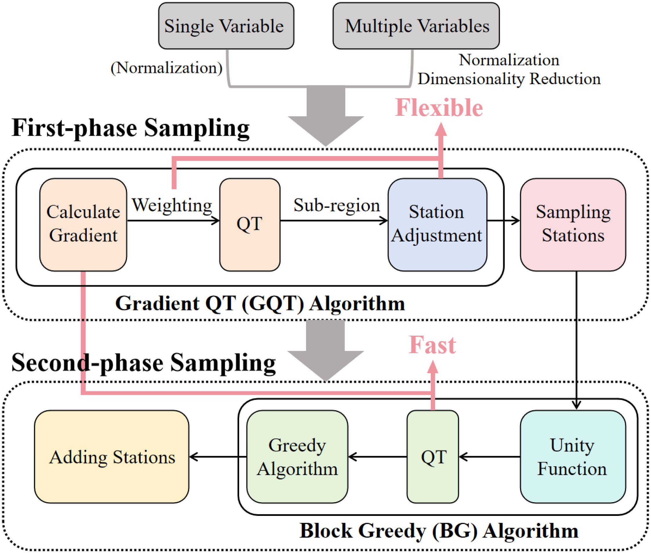
Figure 1 The logical schematic figure that describes the methods. The Fast and Flexible are noted.

The GQT algorithm, an improvement of the Variance QT (VQT) algorithm, refines the computation of changes with the objective of accelerating calculations and is able to maintain the sampling quality. The procedure encompasses the computation of gradients, quadtree decomposition, and station adjustment in sub-region.

The BG algorithm amalgamates the principles of the Greedy algorithm with quadtree decomposition to circumvent redundant computations that arise from the sequential addition of sampling stations. The related steps include the computation of the utility function, quadtree decomposition, and greedy sampling within sub-regions.

Subsequent sections will provide a detailed exposition of the processes involved in these two algorithms. Section 2.1 introduces two algorithms for first-phase sampling: the traditional VQT method, and the GQT method recommended in this article. Section 2.2 introduces the second-phase sampling method. In this section, three utility functions are compared, and then the BG algorithm is proposed to achieve fast sampling. Section 2.3 introduces the method of dealing with the problem of long-term multi-variable sampling. Section 2.4 briefly introduces the reconstruction tool, Kriging interpolation method, used to test the sampling effect.

2.1 First-phase sampling methods

2.1.1 The VQT algorithm

The QT algorithm is a hierarchical decomposition technique that divides a two-dimensional area into four equal-sized strata. This process is repeated iteratively until each stratum meets some criterion of homogeneity. QT algorithm is widely used in the structuring of spatial data, image and data compression, spatial sampling design, grid division, and even path planning (Csillag and Kabos, 1996; Poveda and Gould, 2005; Minasny et al., 2007; Huo et al., 2019; Jiang et al., 2020; Jewsbury et al., 2021; Lee et al., 2021).

The VQT algorithm is based on the principle of QT decomposition, where an area of interest is divided into sub-regions that have more-or-less equal variation (McBratney et al., 1999, 2003). In the process of decomposition, the sub-region with the largest variance is selected for subsequent QT decomposition, and the process is iterated until a certain threshold is reached. The threshold can be total number of sub-regions, variance value, or number of iterations. The variance $Q_h$ within sub-region $h$ is defined in Equation (1).

$\begin{array}{ll}\begin{array}{c}{Q}_h=\sqrt{\frac{1}{2}{\displaystyle \sum _{i=1}^{n_h}{\displaystyle \sum _{j=1}^{n_h}{[z(x_i)-z(x_j)]}^2}}}\end{array}& (1)\end{array}$

where $n_h$ is the number of model grid points, $x_i$ and $x_j$ represent the location in sub-region $h$, and $z$ is the variable of interest.

If we assume that the change in spatial variation is not high [(Minasny et al., 2007), we can use the simplified form Equation (2)] as the splitting criterion.

$\begin{array}{ll}\begin{array}{c}{Q}_h=n_h\sqrt{\frac{1}{n_h-1}{\displaystyle \sum _{i=1}^{n_h}{[z(x_i)-\overline{z_h}]}^2}}\end{array}& (2)\end{array}$

where $\overline{z_h}$ is the mean value of the variables in the sub-region.

The VQT algorithm has several features, as listed in the following aspects.

Consideration of spatial changes. It takes into account the change in variables and places more sampling stations in areas where the spatial variance is large, which consequently optimizes the spatial sampling scheme.

Few parameters. It requires only the number of iterations as a parameter and does not assume any form of spatial covariance function, or isotropy.

Widely adaptable. It can be carried out in irregular areas, which allows it to be sampled in a realistic and complex environment. Besides, it can reasonably arrange the sampling stations according to the cost, without the limit on the number of stations as is often the case with systematic sampling. It can also be extended to multi-variable sampling to adapt to various sampling needs.

However, the VQT algorithm also has some deficiencies:

Repeated calculation. During calculation, even if the simplified form is used, it is still necessary to calculate the variance $n$ times in $n$ iterations.

Ignores arrangement. The algorithm cannot reasonably compare areas with different arrangements but the same elements. Taking two one-dimensional arrays, [1,2,3,4,5] and [1,4,3,2,5], as an example, the variance of these two arrays is the same, but the former is easier to predict than the latter because there is a clear linear trend in the former.

Constrained relative weighting. Spatial sampling tries to find a balance between the two principles of geometric coverage being as reasonable as possible and capturing as much variation as possible. The VQT algorithm will obtain a fixed sampling scheme for a certain variable field, which is designed to minimize the variance and thereby improve the overall reconstruction result. However, a fixed scheme is not conducive to adjustment for different sampling goals and sampling objects.

We aspire to achieve a sampling algorithm where the relative weighting between these two principles can be adjusted at will. Given the strong spatial correlation often exhibited by desired variables, we propose for the QT algorithm an adjustable relative weighting between the two independent indicators—the rate of variable change and the size of the sub-region.

Here, the relative weighting is defined as $\theta =\frac{l}{m}$, where $l$ is the exponent of the variable’s rate of change and $m$ is the exponent of the area of the sub-region. It is envisioned that a sufficiently large range should be encompassed by $\theta$ (ideally, $\theta \in (0,+\infty )$ to guarantee that $\theta$ can accommodate the optimal relative weighting for different variables.

The variance of the VQT algorithm integrates the rate of change and distance (sub-region area). It is postulated that the variable’s change is positively correlated with the rate of change and a certain function $f(d)$ of the distance. Further, it is assumed that the rate of change within the sub-region remains stable, as ${\alpha }_h$. Upon further summation of $f(d)$, it can be represented as a function $F(n_h)$ concerning the area $n_h$ of the sub-region. That is,

$\begin{array}{ll}{Q}_h\sim \sqrt{{\displaystyle \sum _{i=1}^{n_h}{\displaystyle \sum _{j=1}^{n_h}{[{\alpha }_{h}f(d_{ij})]}^2}}}={\alpha }_h\sqrt{{\displaystyle \sum _{i=1}^{n_h}{\displaystyle \sum _{j=1}^{n_h}{f}^2(d_{ij})}}}={\alpha }_{h}F(n_h)& (3)\end{array}$

Furthermore, given that variation is typically positively associated with distance in Equation (3) (the greater the separation between variables, the more significant the change), if $F(n_h)$ is approximated as a power function with $n_h$ raised to the exponent $p$, $p$ is generally greater than $1$. Therefore, the relative weighting $\theta$ will be fixed at $\frac{1}{p}$, with the range being 0–1.

General sampling results. The algorithm only gives a final series of sampling areas and does not specify where in these areas to sample. Typically, sampling stations are simply randomly sampled within an area or are habitually placed in the center of the area.

2.1.2 The GQT algorithm

To solve the above deficiencies and retain the advantages of the VQT algorithm, a new indicator $Q_h^{\text{'}}$ in the QT is defined in Equation (4)

$\begin{array}{ll}\begin{array}{c}{Q}_h^{\text{'}}={\displaystyle \sum _{i=1}^{n_h}{Q}^{\prime }{(x)}^k}\end{array}& (4)\end{array}$

where $k$ is a parameter controlling the importance given to the $Q^{\prime }(x)$ meaning the relative weight of variation, and

$\begin{array}{ll}\begin{array}{c}{Q}^{\prime }(x)=\left|G_x\right|+\left|G_y\right|\end{array}& (5)\end{array}$

$\begin{array}{ll}{G}_x=\left[\begin{array}{ccc}-1& 0& 1\\ -2& 0& 2\\ -1& 0& 1\end{array}\right]\ast (zx),G_y=\left[\begin{array}{ccc}-1& -2& -1\\ 0& 0& 0\\ 1& 2& 1\end{array}\right]\ast z(x)& (6)\end{array}$

Here, $G_x$ and $G_y$ are the gradients of variables along the horizontal direction and the vertical direction, respectively, obtained by convolving the Sobel operator with $z(x)$. It should be noted that the missing parts need to be interpolated and the initial field needs to be expanded by one pixel in each direction to ensure convolution can be performed and the result is the same size as the origin. This method is often used to detect image edges (Mlsna and Rodríguez, 2009; Nixon and Aguado, 2012; Jana et al., 2021). Since $Q^{\prime }(x)$ is the gradient magnitude of the variable, this method is referred to as the GQT algorithm.

The GQT algorithm considers the variation of the chosen variable. Meanwhile, since only the variation indicator has changed, the GQT algorithm is simple in form and can be adapted to a variety of sampling requirements, retaining the various advantages of the VQT algorithm.

However, the difference is that the GQT algorithm only sums the gradient magnitude in the selected area during the iterative process, avoiding repeated calculations of the variation indicator, which is expected to save a considerable amount of calculation time. At the same time, the gradient magnitude gives the variable’s rate of change at each position, which allows the algorithm to distinguish between areas with the same elements but more irregular arrangements.

Moreover, because the changing rate and distance are independent of each other, the GQT algorithm can adjust the relative weights freely to accommodate the sampling of different variables. When $k$ is large, the algorithm will prioritize variation, making it suitable for hotspot detection. Conversely, a small $k$ will result in more evenly distributed sampling stations. If $k=0$, the algorithm will be similar to systematic sampling, which can be applied to the first-phase sampling of unknown variable fields. To align with VQT and optimize the reconstruction error, $k$ should assume an appropriate value within 0–1. To propose a suitable weight for the prior, we assume a sufficiently large square sub-region where variable variation is linearly related to distance. Then,

$\begin{array}{ll}\begin{array}{c}F(n_h)=\sqrt{n_h{}^3(1-\frac{1}{n_h})}\approx n_h{}^{\frac{3}{2}}\end{array}& (7)\end{array}$

and $k$ is adjusted to $\frac{2}{3}$ accordingly [Supplementary Material provides specific derivation procedures for Equation (7)].

Using the gradient magnitude field can further guide the adjustment of sampling stations: the gradient field $Q^{\prime }(x)$ obtained based on Equation (5) and Equation (6) can be regarded as “density”, and the sampling stations are adjusted to the center of gravity $s_h{}^{\text{'}}$ of the region, as shown in Equation (8).

$\begin{array}{ll}\begin{array}{c}{s}_h^{\text{'}}=\frac{{\displaystyle {\sum }_{i=1}^{n_h}{Q}^{\prime }(x_i{)}^k{x}_i}}{{\displaystyle {\sum }_{i=1}^{n_h}{Q}^{\prime }(x_i{)}^k}}\end{array}& (8)\end{array}$

In this paper, the GQT algorithm after station adjustment (GQT-ad) only performs station adjustments on sub-regions whose average gradient magnitude is greater than 80% of the gradient magnitude in the whole area ($\overline{Q^{\prime }(x)}+0.84\sigma (Q^{\prime }(x))$), to ensure that when variation is weak, more attention is paid to achieving a uniform spatial distribution.

2.2 Second-phase sampling methods

2.2.1 Utility function

Second-phase sampling is defined as adding new samples to existing ones to improve the overall estimate of the variable of interest, the aim of which is to collect new samples to minimize prediction error. Therefore, the goal of second-phase sampling is to find a suitable indicator and reduce this indicator as much as possible when adding new sampling stations.

Kriging variance ${\sigma }_{KV}{(x)}^2$ is one of the commonly used indicators. It provides the uncertainty of prediction and can be expressed as

$\begin{array}{ll}\begin{array}{c}{\sigma }_{KV}{(x)}^2={\sigma }^2-c^T(x)C^{-1}c(x)\end{array}& (9)\end{array}$

where $C^{-1}$ is the inverse matrix of the covariance matrix $C$ based on the covariance function, $c$ is a column vector, and $c^T$ is its corresponding row vector.

However, the kriging variance assumes a stationary variable but does not take into account the real variation of the variable. Therefore, the introduction of weighted kriging variance helps to better select new sampling stations (Delmelle and Goovaerts, 2009), as follows:

$\begin{array}{ll}{\sigma }_{WKV}{(x)}^2=w{(x{)}^{\lambda }}^{}{\sigma }_{KV}{(x)}^2.& (10)\end{array}$

Here, $w(x)$ is the weight and $\lambda$ is a parameter controlling the importance given to the weight. When $\lambda$ is 0, Equation (10) degenerates into Equation (9). In this paper, the weight uses the gradient field $Q^{\prime }(x)$ obtained by Equation (5), and $\lambda$ is set to 1.

With the help of the presence of simulation output or satellite data, another effective method is to directly subtract the predicted field $z_f(x)$ obtained through the first-phase sampling stations from the model simulation field $z(x)$ to obtain the error field $e(x)$. $e(x)$ shown in Equation (11) is equivalent to adaptively selecting a suitable value of $\lambda$ so that it can be a feasible substitute for the weighted kriging variance:

$\begin{array}{ll}\begin{array}{c}e(x)=\left|z(x)-z_f(x)\right|\end{array}& (11)\end{array}$

2.2.2 The BG algorithm

Upon acquiring the error field, the set of potential sampling locations for the spatial search may be extensive. For instance, in the studied area, with 992 valid grid points, the number of possible combinations from adding 5 new stations to the 20 sampling stations (according to the first-phase sampling) can reach 7.16 × 10¹². To find satisfactory solutions in this vast solution space, leveraging different algorithms is necessary. Typically, a fast heuristic algorithm, such as the greedy algorithm, is applied firstly to obtain an acceptable sampling scheme. If higher quality is required for the sampling scheme, iterative algorithms, such as simulated annealing or genetic algorithms, can be used to further optimize the existing scheme towards an optimal solution. The greedy algorithms can be employed in the design of second-phase sampling since they can provide a satisfactory final scheme, serve as a starting solution for iterations, or act as a benchmark for other heuristic algorithms.

For problems that require adding $n$ new sampling stations, taking the error field as an example, the greedy algorithm searches the first $n$ positions with the largest current error for sampling. However, since the error is often spatially correlated, the results obtained in this way are likely to cause the new stations to cluster together, thus obtaining poor results. Therefore, a dynamic greedy (DG) algorithm (sequentially added greedy algorithm) is generally used for second-phase sampling (Rogerson et al., 2004). The DG algorithm adds one sampling station at the position with the maximum error in the error field each time and recalculates the error field. As a result, the DG algorithm can flexibly arrange stations based on utility functions. This process is repeated until the required number of samples $n$ is reached. This method can make the distribution of new sampling stations more reasonable to optimize the second-phase sampling, but the number of calculations also increases to $n$.

To achieve a reasonable distribution of new sampling stations while reducing the number of calculations, the BG algorithm is used in this study. This method uses the QT algorithm to divide the research area into sub-regions, then uses the greedy algorithm to sample in each sub-region. For a second-phase sampling task of adding $n$ sample stations, the specific steps are:

(1) Divide the irregular research area into multiple sub-regions with similar areas through the QT algorithm.

(2) Determine whether the threshold is met. In this study, it is required that the number of sub-regions is not less than $n$, the standard deviation of the sub-regions is sufficiently small, and the sub-region with the $n$th largest average error is required to be greater than the average error of the entire study area. Step 1 will be repeated until the above requirements are met.

(3) Select the top $n$ sub-regions with the largest total error among these sub-regions and use the greedy algorithm for sampling.

In this way, the error field only needs to be calculated once, and the new sampling stations will not be clustered together.

2.3 Long-term and multi-variate sampling methods

In reality, observation systems often need to perform observation tasks for a certain time scale, and need to perform observations of multiple variables. Therefore, a multi-variable sampling scheme that is suitable for long-term observations is necessary.

In multivariate sampling, integrating information from multiple variables and finding their common characteristics is a key step. Proposed methods include performing the principal component analysis (PCA; Hengl et al., 2003; Aquino et al., 2014), creating a Latin hypercube of the variables (Minasny and McBratney, 2006; Erten et al., 2022), calculating Eigen-Entropy (Huang et al., 2023), and measuring pointwise mutual information (Dutta et al., 2019).

Two feasible multivariate sampling solutions for the GQT algorithm are provided, and both solutions need normalize the variables (i.e., remove the mean and divide by the standard deviation) at the first step. After that, the first solution involves calculating the variation of each normalized variable and performing a weighted linear combination. The second solution involves performing PCA on normalized variables and calculating the variation using corresponding mode of the first principal component.

In this study, we use the second approach to reduce time cost since the gradient is calculated one time only. This can avoid calculating the spatial variation for all variables. Moreover, for multi-variable sampling under a time series, the indicator is adjusted to

$\begin{array}{ll}\begin{array}{c}{Q}_h^{\ast }={\displaystyle \sum _{t=1}^T{\displaystyle \sum _{i=1}^{n_h}{Q}^{\ast }{(x}_i, {t)}^k}}\end{array}& (12)\end{array}$

In Equation (12), $T$ is the time series length, and $Q^{\ast }{(x}_i, t)$ is the variation indicator calculated on corresponding mode of the first principal component.

2.4 Interpolation method

After obtaining the sampling stations, Kriging interpolation is used to interpolate and predict the variables (using the PyKrige package in Python). Also, the method is selected as OrdinaryKriging, and the variogram is selected as “spherical”.

3 Results

In this section, the northern Bay of Bengal is chosen as a study case to gain insights into the application of sampling algorithms. In addition to testing the sampling effect of the algorithm, the sampling design in the northern Bay of Bengal also has practical and scientific value.

The oceanic surface environment (such as the SST and SSS) in the Bay of Bengal can affect the formation of tropical cyclones, which the addition of in situ data can help to accurately understand. SST and SSS data in the northern Bay of Bengal (15°–22°N, 80°–98°E) in 2022 are chosen to demonstrate the application of this algorithm. The SST data used are from NOAA’s 1/4° Daily Optimum Interpolation Sea Surface Temperature (OISST) dataset, and the SSS data are from ESR’s 1/4° 7-day Optimum Interpolation Sea Surface Salinity (OISSS) dataset. In addition, since ocean velocity is also an important research variable, we also add surface zonal and meridional velocities (U and V) in the long-term multivariable experiment. The 1/4° daily surface velocity data used are from “Sea level gridded data from satellite observations for the global ocean from 1993 to present” (Copernicus Climate Change Service, Climate Data Store, 2018). To ensure temporal consistency among the four sets of data, the SST, U, and V data are averaged over a 7-day time scale starting from 2 January 2022, and output at 4-day intervals. Consequently, four sets of data are obtained with a time dimension of 91 and a spatial dimension of 28 × 69.

Figures 2A, B show the SST and SSS fields in the first week of 2022 (2021.12.30 to 2022.1.5), while Figures 2C, D show the corresponding spatial gradient fields, reflecting the spatial distribution of variable change rates. The spatial gradient fields show that the steepest changes in SST occur in the northern and northwestern coastal parts of the region, while changes in SSS occur in the southeastern region and a “Z”-shaped region running from north to south near 91°E.

Figure 2

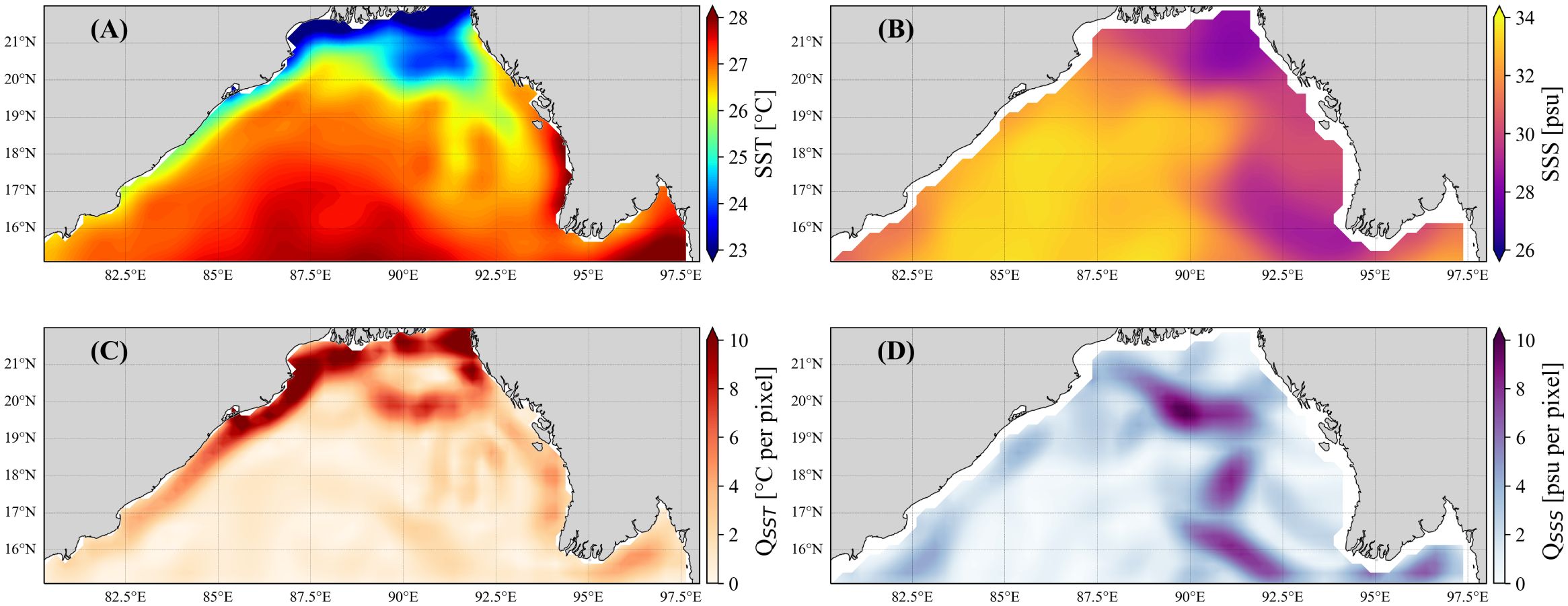
Figure 2 (A) SST field in the first week and (C) the corresponding spatial gradient field. (B, D) As in (A, C) but for SSS.

Below, we conduct a quantitative analysis of the sampling efficiency and quality of the GQT algorithm and the BG algorithm. Furthermore, we design a long-term bivariate first-phase sampling and second-phase sampling scheme with practical application value.

3.1 Fast spatial sampling scheme

The GQT algorithm circumvents the need for repeated utility function calculations (e.g., spatial gradient or error), resulting in O(1) time complexity (only considering the calculation time of utility function). Figure 3 provides a quantitative comparison of calculation times across different sampling algorithms.

Figure 3

Figure 3 (A) Time consumption of the sampling based on SST to obtain 150 stations by using VQT (purple), simplified VQT (green), and GQT (red). (B) Time-consumption ratio of VQT to GQT (purple) and that of simplified VQT to GQT (red). (C) The ratio of the time consumption of calculating the utility function to its total time consumption using VQT (purple), simplified VQT (green), and GQT (red). (D) Time consumption of DG (purple) and BG (red). (E) The time-consumption ratio of the two (red), in which the black dotted line is the reference line with a slope of 1.

In the first-phase sampling design, the VQT algorithm takes about 19 seconds to obtain 150 sampling stations for SSS in the study area with a time dimension of 91 (Figure 3A), with the utility function calculation accounting for over 99% of the total sampling time (Figure 3C). Simplifying the VQT algorithm reduces the sampling time to approximately 2.5 s. Still, the proportion of time dedicated to the utility function calculation remains stable at about 95%. Therefore, optimizing the utility function calculation method is key to reducing the calculation time efficiently. With the GQT algorithm, obtaining 150 sampling stations takes less than 0.5 s, which is 1/40 the time of the VQT algorithm and 1/5 the time of the simplified VQT algorithm (Figure 3B). Due to significantly reducing the time cost, the fast sampling design is achieved. Obtained from 5 to 150 sampling stations, the calculation time remains almost unchanged. This implies that the sampling process is fast for a large number of stations. In general, the GQT algorithm has the advantage of fast sampling, and this advantage can be maintained in large sampling tasks.

In the second-phase sampling, the DG algorithm’s time consumption increases linearly, while the BG algorithm, with its O(1) time complexity, greatly reduces the time consumption when adding a large number of sampling stations. Therefore, both the GQT and BG algorithms significantly enhance the sampling efficiency and are beneficial for large-scale sampling.

While the time consumption in this example is only several seconds and entirely manageable, the advent of higher-resolution simulations or satellite data and broader exploration areas in the future will significantly increase the overall time required for sampling. Furthermore, the increasing frequency and intensity of future field observation studies will underscore the importance of rapid sampling. These methodologies hold potential application value for ocean detection and spatial sampling tasks across various fields.

3.2 Sampling results

3.2.1 Sampling quality based on the GQT algorithm

As the goal of fast sampling is achieved, the reconstruction results after sampling are examined. The sampling of SST and SSS based on the VQT algorithm (Figures 4A, B) and GQT-ad (k = 2/3, Figures 4C, D) is initially presented. As demonstrated, the overall sampling results are akin to the VQT algorithm, with dense sampling in areas of large variation.

Figure 4

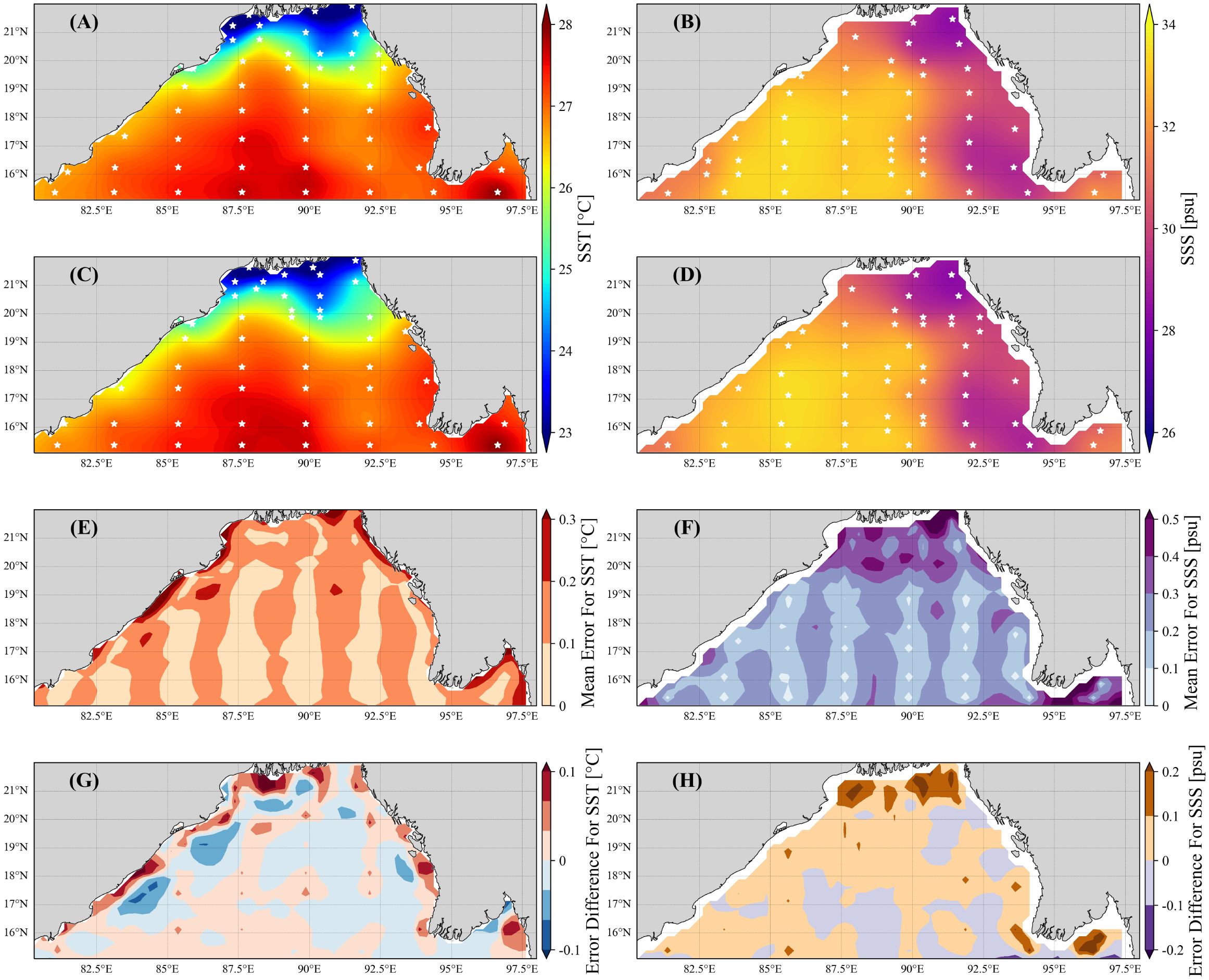
Figure 4 The reconstructed (A) SST and (B) SSS fields in the first week using VQT. (C, D) As in (A, B) but using the GQT algorithm after station adjustment (GQT-ad, k = 2/3). White points represent the 50 sampling stations. (E) Average SST error field and (F) average SSS error field using GQT-ad. (G) Difference between the average SST error fields of VQT and GQT-ad. (H) As in (G) but for SSS.

Figures 4E, F further illustrate the spatial distribution of average error from using GQT-ad. For SST, the error in most areas is controlled within 0.2°C, and only a few coastal areas exceed an error of 0.2°C. For SSS, the error is less than 0.3 psu in most areas, with an error of approximately 0.4 psu only in the northern and eastern parts of the area. In general, the large errors are mainly located far away from the sampling point and in the position with large variation. Compared to the VQT algorithm (Figures 4G, H), GQT-ad has a similar error overall but performs better in locations with greater variation (e.g., the nearshore area for SST and northern parts of area for SSS). This shows that the error in the critical area can be reduced due to the flexible adjustment of the stations. This will induce the relative uniform spatial error distribution.

To further quantitatively analyze the advantages of the GQT algorithm, the root-mean-square error (RMSE) is calculated according to Equation (13).

$\begin{array}{ll}\begin{array}{c}RMSE=\sqrt{\frac{1}{N}{\displaystyle \sum _{i=1}^N{(V_i-\widehat{V_i})}^2}}\end{array}& (13)\end{array}$

Here, $N$ is the total grid points, $V_i$ is the original data value, $\widehat{V_i}$ is the reconstructed value. Figures 5A, B show the RMSE of the SST and SSS under a range of sampling stations by using random sampling, the VQT algorithm (The results obtained by the simplified VQT algorithm are basically the same as the VQT algorithm. SM, Supplementary Figure 1), and the GQT algorithm (including GQT-ad, k = 2/3). Compared with random sampling, both the VQT and GQT algorithms optimize the RMSE greatly, especially when stations are sufficient. When the number of stations exceeds 25, the RMSE of the SST and SST fields reconstructed by the VQT and GQT algorithms are significantly reduced. (Initially, the normality of RMSE was tested, and it was found that the majority of the data did not adhere to a normal distribution. SM, Supplementary Table 1. Consequently, the one-sided Mann-Whitney U test was utilized to conduct the significance test, α = 0.05. SM, Supplementary Table 2).

Figure 5

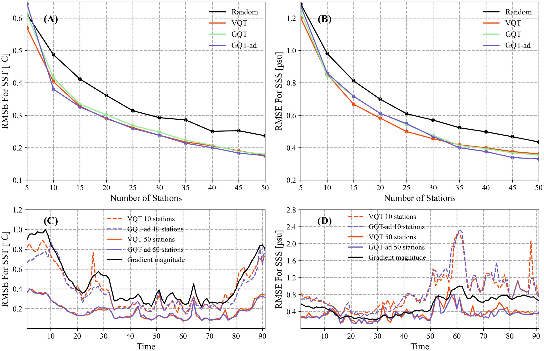
Figure 5 The RMSE of the (A) SST and (B) SSS reconstruction versus the number of stations by using random sampling (black), VQT (red), GQT (green), and GQT-ad (purple). The RMSE of the (C) SST and (D) SSS reconstruction versus time under 10 (dashed line) and 50 (solid line) sampling stations by using VQT (red) and GQT-ad (purple). The black solid line is the averaged spatial gradient.

The GQT algorithm and the VQT algorithm yield similar reconstruction effects for both SST and SSS, with no significant difference between them (The two-sided Mann-Whitney U test is used to perform the significance test, α = 0.05. SM, Supplementary Table 3). The GQT algorithm shows a slightly worse reconstruction result than the VQT algorithm, increasing the average RMSE by about 2%. After station adjustment, the RMSE difference is lower than 0.4%. In addition, with the help of station adjustment, GQT-ad performs better when the number of stations is larger, reducing the average RMSE by 1.9% for SST and 5.1% for SSS. Combined with the comparison with random sampling, it indicates that emphasis putting on variation can effectively reduce errors only when there are sufficient sampling stations. Although GQT-ad does not show obvious optimization on the whole, flexible station adjustment has become a non-negligible advantage of GQT-ad in locations with sufficient sampling stations and large variation.

Moreover, the adjustable and flexible attribution of the GQT algorithm allows for potential improvement in the reconstruction field by selecting a more suitable k. For instance, SST variation is primarily concentrated in a small coastal area, which may limit the algorithm’s ability to capture it. Therefore, increasing k could yield better results. This is indeed observed when adjusting k. Compared to when k=2/3, increasing k to 1 results in a reduction of the average RMSE by 0.4%. However, if k is decreased to 1/2, the average RMSE appears an increase of 1.1%. In the case of SSS, the area of significant variation extends from north to south near 91°E, which may overemphasize the change. Consequently, reducing k could amplify the effect. Similarly, when k is decreased to 1/2, the average RMSE reduce by 0.3%, but an impressive increase of 4.5% is observed when k is increased to 1.

The RMSE exhibits distinct variations across different periods (Figures 5C, D). A notable deterioration in the reconstruction efficacy of SST is evident during the winter months, while the reconstruction of SSS appears to be significantly compromised in the summer and autumn seasons. Interestingly, the augmentation of sampling stations primarily diminishes the RMSE during periods of high RMSE values, yet this reduction is less pronounced during periods characterized by lower RMSE. This suggests a potential need for an increased number of samples during periods with larger RMSE to meet the requisite threshold. And conversely, a reduction in sample size is acceptable during periods with smaller RMSE to circumvent unnecessary expenditures.

Furthermore, it is important to note that fluctuations in RMSE are strongly correlated with changes in spatial gradient (At 10 stations, the correlation coefficient exceeded 0.95 for SST and 0.84 for SSS). This correlation can be instrumental in providing preliminary guidance for the sampling scheme.

3.2.2 Long-term multi-variate sampling scheme

In practical applications, it is essential to consider the information on SST and SSS over a given period for the design of the sampling scheme. The first principal component, derived from PCA, accounts for an average of 68.7% of the variance and is utilized in the computation of the utility function. Figure 6A illustrates the joint spatial gradient, which encapsulates the long-term comprehensive variation distribution of SST and SSS. Notably, significant variations are observed along the northwest coast, northern region, and southeastern part of the area under study. Decomposing this distribution of variation yields the sampling scheme of the GQT algorithm.

Figure 6

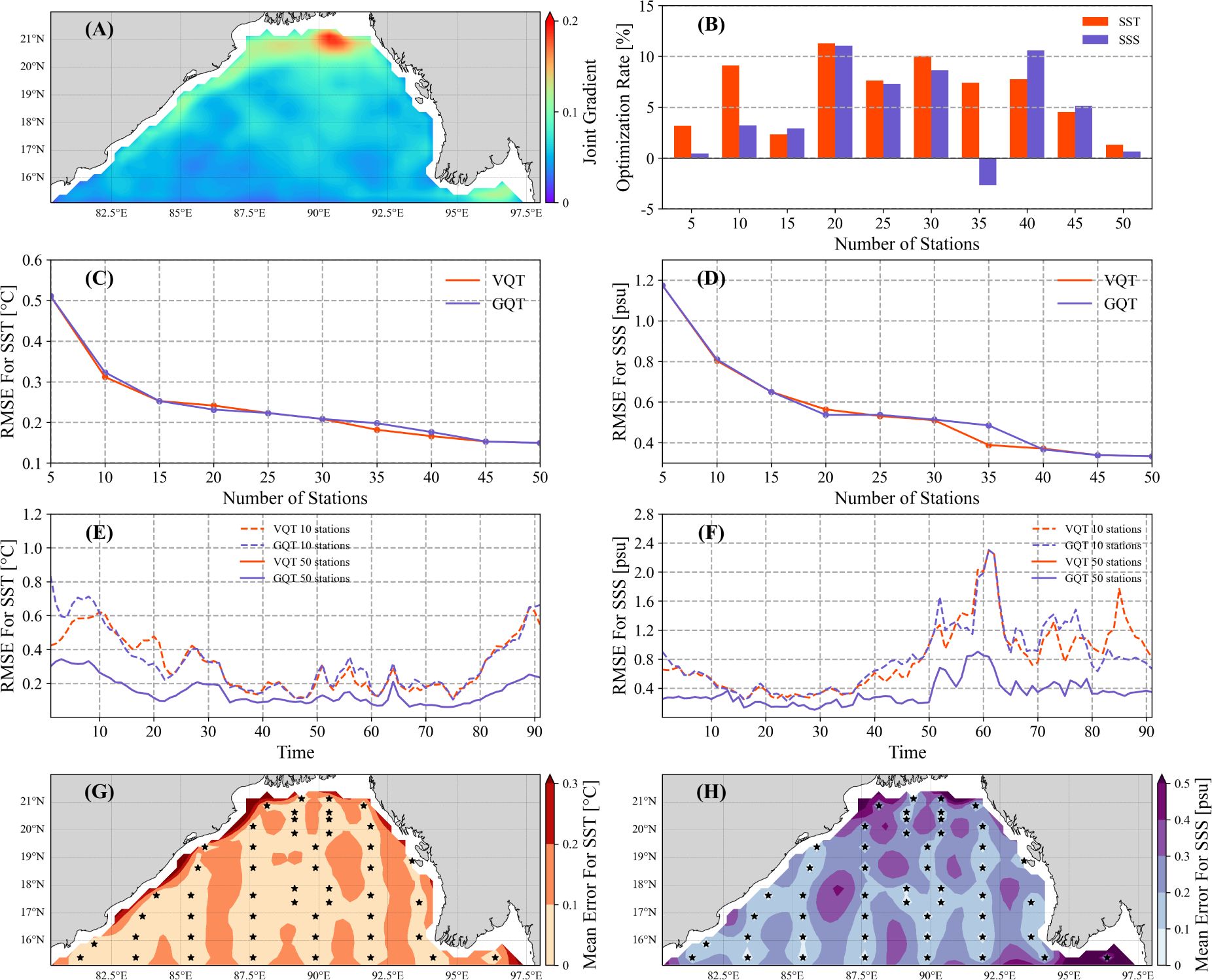
Figure 6 (A) The average joint spatial gradient of the corresponding mode of the first principal component. (B) The average RMSE optimization of the long-term bivariate sampling scheme in GQT compared to only considering one variable in GQT. The RMSE of the (C) SST and (D) SSS reconstruction versus the number of stations by using VQT (red) and GQT (purple). The RMSE of the (E) SST and (F) SSS reconstruction versus time under 10 (dashed line) and 50 (solid line) sampling stations by using VQT (red) and GQT (purple). (G) Average SST error field and (H) average SSS error field using GQT. The black stars represent 50 sampling stations.

In comparison to the sampling scheme that only considers a single variable (Figure 6B), the prediction that incorporates bivariable information is optimized by an average of 5.6% (with a 6.5% optimization when considering SST and a 4.7% optimization when considering SSS). Figures 6C, D depict the RMSE optimization of the long-term bivariate sampling scheme in the GQT algorithm as compared to the VQT algorithm. On the whole, the reconstruction fields of the GQT algorithm and the VQT algorithm exhibit high similarities.

In the long-term bivariate sampling scheme, the temporal trend of the RMSE (Figures 6E, F) mirrors that depicted in Figures 5C, D. However, a significant decrease in RMSE is observed when the number of stations is minimal and the variation is substantial. Given that the algorithm incorporates weekly changes during long-term sampling, this suggests that during periods of greater variation, the sampling distribution will be more uniform. This further implies that when the sampling budget is constrained (i.e., the number of stations is small), considering variable variations may not be an effective strategy to reduce the reconstruction error, particularly during periods with large variations.

Figures 6G, H presents the sampling scheme, reconstruction field, and error of 50 sampling stations by employing a long-term bivariate sampling scheme based on the GQT algorithm. The sampling stations are densely positioned in the area where the joint spatial gradient is large, as depicted in Figure 6A. The error is effectively controlled within 0.2°C for SST and 0.3 psu for SSS across most regions, which is not obviously larger than that shown in Figures 4E, F, thereby validating the efficacy of this long-term bivariate sampling scheme.

To further test the stability of the algorithm under long-term multi-variable scenarios, zonal and meridional velocities are added (Figure 7). Similarly, simultaneously considering multiple variables can help improve the sampling effect. Compared with only considering a single variable, the average improvement is 3.2% (optimized by 3.4% for SST, 2.6% for SSS, 2.1% for U, and 4.8% for V). The obtained sampling results are comparable to those achieved by the VQT method, with a difference of less than 0.2%.

Figure 7

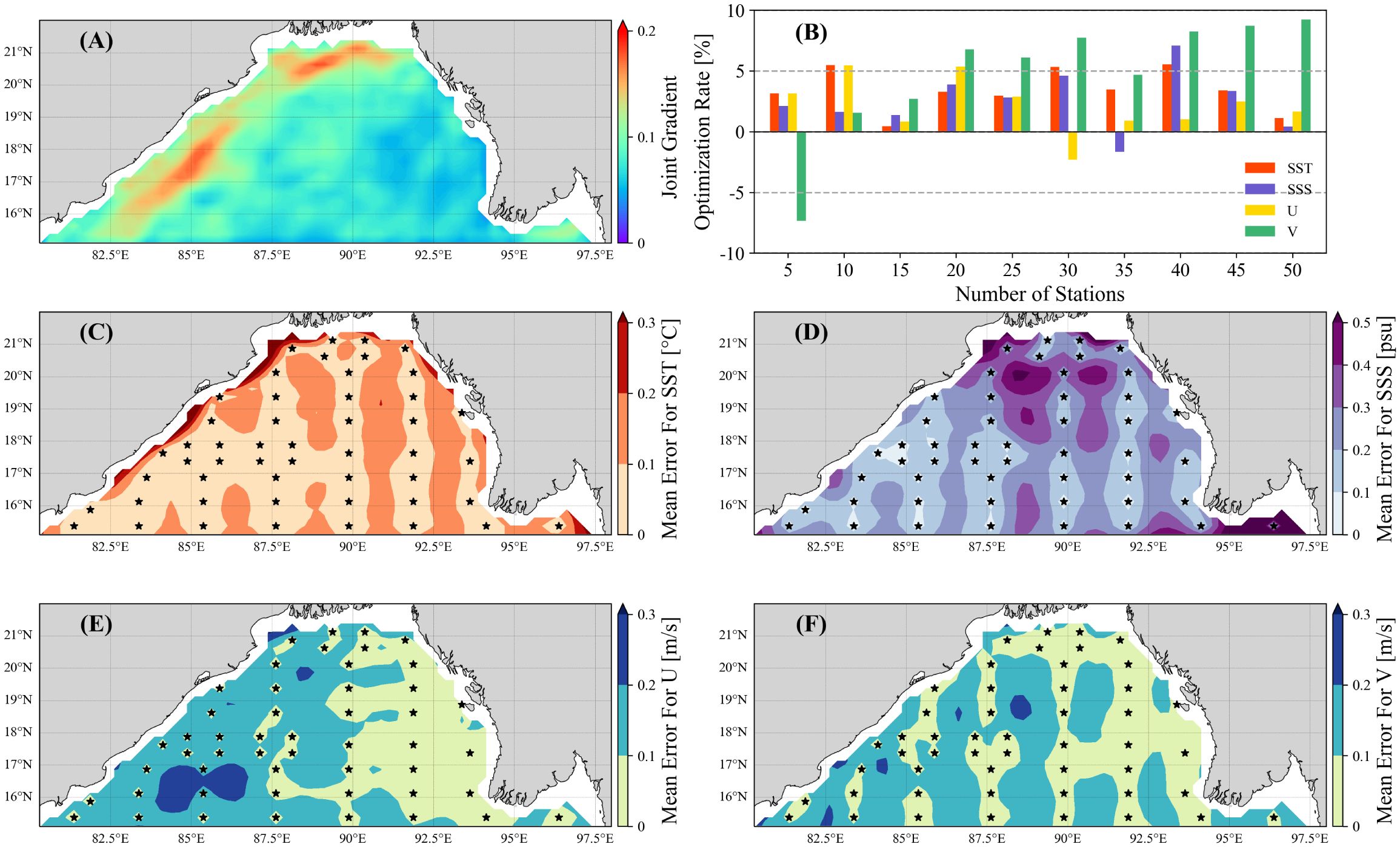
Figure 7 (A) The average joint spatial gradient of the corresponding mode of the first principal component. (B) The average RMSE optimization of the long-term multivariate sampling scheme in GQT compared to only considering one variable in GQT. (C) Average SST error field, (D) average SSS error field, (E) average U error field, and (F) average V error field using GQT. The black stars represent 50 sampling stations.

However, spatial variations of ocean velocity measurements present more complexity, with pronounced anisotropy and heightened variability. As a result, the velocity error in some areas even exceeds 0.2m/s (Figures 7C, D), which means that the flow in this area is not well reconstructed. Thus, a greater number of sampling stations (with 100 sampling stations, the average error of velocity can be reduced to 0.08-0.09 m/s) or more advanced interpolation methods are necessary to ensure reliable reconstruction. In cases where sampling budgets are constrained, methods such as lifting interpolation, as exemplified by the objective analysis method (e.g. OAX, McGillicuddy et al., 2001), can prove especially critical. In addition, the complex spatial structure of velocity makes assimilation in combination with other observation methods particularly important.

3.2.3 Second-phase sampling

Based on the long-term bivariate sampling scheme obtained by the GQT algorithm, a second-phase sampling scheme was further designed. To verify whether the ability of the utility function to optimize the second-phase sampling scheme improves after considering variation, Figures 8A-D display the RMSE optimization of using error-based utility function compared to using Kriging Variance (Figures 8A, B) and Weighted Kriging Variance (Figures 8C, D) as the utility function under a series of first-phase designed stations.

Figure 8

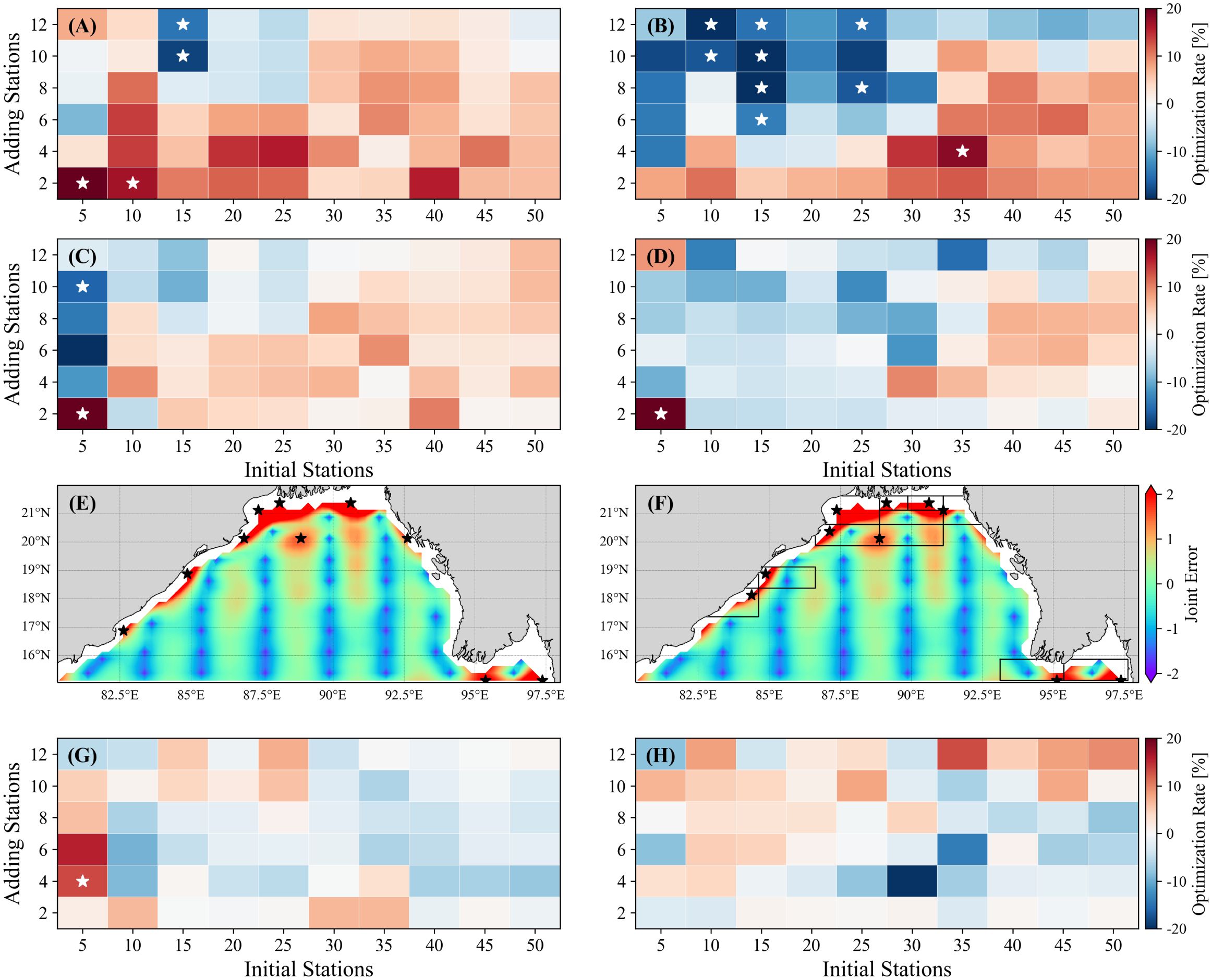
Figure 8 The (A) SST and (B) SSS RMSE optimization rate of ER compared to KV. The (C) SST and (D) SSS RMSE optimization rate of E compared to WKV. (E) The sampling stations based on DG. (F) as in (E), but the sampling stations are based on BG. For (G) SST and (H) SSS, the optimization rate of BG compared to DG with error as the utility function, where the positions of the white stars indicate significant differences between the two RMSEs (using the two-sided Mann-Whitney U test, with α = 0.05).

Qualitatively, as mentioned before, when the number of stations is limited, a reasonable spatial distribution becomes more critical and may even emerge as the primary determinant of the error. Consequently, utilizing error as a utility function yields unsatisfactory results when the number of initial stations is limited. However, as the quantity of initial stations reaches an adequate level, the benefits of this approach become increasingly evident. In other words, the error-based utility function is suitable for second-phase sampling tasks with adequate initial stations.

Figures 8E, F present the sampling scheme for adding 10 stations to the 40 first-phase designed stations by using the DG and BG algorithm. Since there are enough initial stations, error is used as the utility function here. The BG algorithm enables the sampling stations to achieve a reasonable spatial distribution while capturing the maximum error. Compared to the distribution obtained by the DG algorithm, 6 out of the 10 stations are identical. It implies that the BG algorithm can enhance efficiency while also maintaining flexibility of the Greedy algorithm.

To systematically evaluate the performance of the BG algorithm against the DG algorithm, Figures 8G, H display the RMSE optimization of the BG algorithm under a series of first-phase designed stations. When compared to the DG algorithm under the error-based utility function, the overall reconstruction error increases by 0.5%. The reconstruction of SST shows an overall deviation, with an increase of 2.7% in RMSE, while the reconstruction of SSS optimizes by 1.7%. Therefore, compared with the DG algorithm, although the calculation time is greatly reduced, the sampling results are still at the same level. Additionally, when the initial number of stations is limited, the BG algorithm has a slight advantage. This reflects the improvement of globality brought by the use of quadtree decomposition. As a combination of quadtree decomposition and the Greedy algorithm, the BG algorithm can achieve the fast and flexible sampling scheme, which successfully combines the advantages of both.

4 Discussions

Spatial variation of variables is an important feature. Capturing the variation in variables as much as possible is therefore one of the principles of spatial sampling. Many spatial sampling schemes also rely on measures of change, such as entropy, variance, or, as mentioned in this study, gradient. After considering the changes in variables, more satisfactory results were indeed obtained.

However, for a sampling scheme that aims at interpolation reconstruction, the change information of variables can be reflected not only by the interpolation points themselves but also by the changes between interpolation points. In other words, to accurately capture the changes in variables, the sampling points should be distributed more evenly in the areas with large changes, rather than specific locations. Ideally, the sampling scheme should first identify the areas with larger changes and allocate more sampling points to them. Then, the sampling points should be located at the positions that can best depict the changes in the variables (for example, the positions where the changes start to increase or decrease rapidly), rather than the positions with the maximum change. This requires that the utility function in the algorithm can reflect the areas with large changes at the macro level, as well as capture the valuable sampling points, such as extreme points, at the micro level.

Using the Laplacian operator to obtain the spatial second derivative of the variable and applying it to QT decomposition may be a feasible method to achieve this goal (Equation (14) and Equation (15). Since this algorithm uses the gradient of the gradient as the criterion for QT decomposition, it is later called the GGQT algorithm. Here,

$\begin{array}{ll}\begin{array}{c}{Q}_{h-new}^{\text{'}}={\displaystyle \sum _{i=1}^{n_h}{Q}_{new}^{\text{'}}{(x)}^k}\end{array}& (14)\end{array}$

$\begin{array}{ll}{Q}_{new}^{\text{'}}(x)=\left[\begin{array}{ccc}-1& -1& -1\\ -1& 8& -1\\ -1& -1& -1\end{array}\right]\ast z(x)& (15)\end{array}$

Similarly, the adjustment of the sampling station changes as shown in Equation (16).

$\begin{array}{ll}{s}_{h-new}^{\text{'}}=\frac{{\displaystyle {\sum }_{i=1}^{n_h}{Q}_{new}^{\text{'}}(x_i{)}^k{x}_i}}{{\displaystyle {\sum }_{i=1}^{n_h}{Q}_{new}^{\text{'}}(x_i{)}^k}}.& (16)\end{array}$

When the spatial second-order derivative of a certain position is large, it means that the change in position is larger. Compared with the first-order derivative, it will sample at a position closer to the extreme point rather than the position with the largest change. At the same time, it also means that there are areas of greater change nearby. This method meets the above requirements and may achieve better sampling results.

Figures 9A, B depict the spatial second-order gradient, which is more pronounced around the nearshore location in the SST and the “Z”-shaped region in the SSS. A sampling scheme is subsequently derived through QT decomposition. Figures 9C, D present the sampling results of 50 stations, demonstrating that the stations are indeed more densely populated in areas with significant variable changes. However, the sampling stations tend to be more dispersed around areas exhibiting high values of variation. To quantitatively evaluate their impacts, the RMSE of both the GGQT algorithm and the GQT algorithm are compared (Figures 9E, F). The RMSE of SST based on GGQT-ad shows a decrease of 3.6% on average compared to GQT-ad. Similarly, that of SSS decreases by 2.6%. In terms of the spatial distribution of errors (Figures 9G, H), GGQT-ad shows significantly better results in some regions, such as the northwest shore (19°N, 85°E) for SST and the southeast part (15.5°N, 97.5°E) for SSS. At the same time, compared with VQT, GGQT-ad is optimized by 3.1% on average. In addition, since only one convolution kernel is used, the GGQT algorithm will be faster than the GQT algorithm.

Figure 9

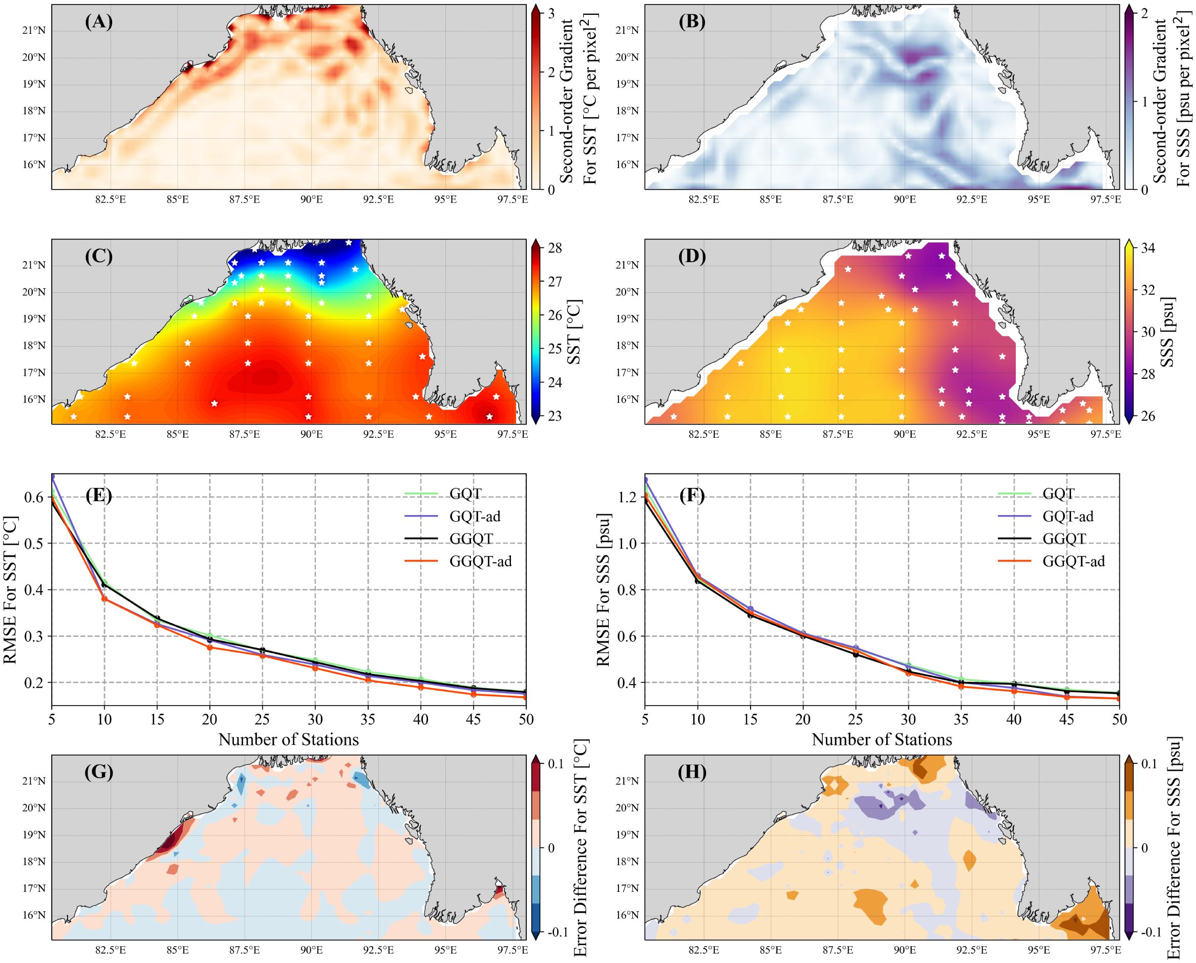
Figure 9 (A) Second-order spatial gradient field of SST in the first week. (B) As in (A) but for SSS. The (C) SST and (D) SSS reconstruction fields in the first week using GGQT-ad, where white points represent the 50 sampling stations. The RMSE of the (E) SST and (F) SSS reconstruction versus the number of stations by using GQT (green), GQT-ad (purple), GGQT (black), and GGQT-ad (red).

These findings suggest that the proposed algorithm effectively enhances the reconstruction result, thereby demonstrating its significant application value. However, since it is challenging to find a corresponding theory for adjusting the relative weight k in the GGQT algorithm, the value of k = 2/3 is retained here in the above comparison. This choice inevitably introduces some subjectivity. Therefore, a future research direction is to explore a theoretically derived pre-given k.

In our future research, there is substantial scope for further enhancements and improvements. Sampling at specific temporal scales can enable observations to address pertinent scientific inquiries more effectively. By filtering variables on either a temporal or spatial scale, a more suitable sampling plan can be devised for distinct scientific challenges (Liu et al., 2018).

Moreover, expanding the sampling algorithm to encompass three-dimensional space and taking into account the vertical variations of variables can facilitate a more comprehensive observation of actual oceanic processes. The utilization of an Octree instead of the Quadtree can address the issue of sub-region segmentation in three-dimensional space. When combined with the fast algorithm presented in this study, it is anticipated that the substantial computational demand of three-dimensional sampling can be mitigated, thereby achieving an efficient and stable design for three-dimensional sampling.

5 Conclusions

In this study, we employed the GQT algorithm, a novel QT sampling method that utilizes the gradient magnitude of variables rather than the variance, to build the first-phase sampling scheme. The GQT algorithm offers several advantages over the VQT algorithm:

(1) The computation time does not significantly increase with the rise in the number of stations, facilitating large-scale multi-station sampling.

(2) It can provide the variation of specific locations, offering more precise guidance for the sampling stations.

(3) It allows for a more flexible allocation of variation weights, adapting to the reconstruction of different variables.

Additionally, the BG algorithm, which employs the QT algorithm to ensure a reasonable spatial distribution and reduce time consumption, can obtain a spatially reasonable sampling scheme with the time complexity of O(1). At the same time, the combination with the greedy algorithm can flexibly arrange the station according to the utility function. It is applied in the second-phase sampling.

Through an example in the Bay of Bengal, we provide a set of sampling schemes based on the aforementioned two algorithms to verify their sampling quality and compare time-consumption. For the first-phase sampling, similar to the VQT algorithm, the reconstruction effect of the GQT algorithm is significantly optimized compared to random sampling. Besides, the GQT algorithm performs slightly better where the variables of interest with large variation, because of the ability to adjust stations in response to variations. By further reducing the excessive focus on change, the GGQT algorithm can be optimized by more than 3% compared to the VQT algorithm. At the same time, the computation time is about 1/40 of that of VQT (at 150 sampling stations in this study). For the second-phase sampling, compared with the DG algorithm, the BG algorithm can control the time consumption to a constant time complexity while ensuring that the sampling effect is comparable.

During the comparison of the algorithms, notable considerations regarding sampling are mentioned. It was observed that the spatial gradient exhibits a strong correlation with the level of error. Adjusting sampling budgets based on spatial gradients is anticipated. Moreover, incorporating variability in study variables does not effectively optimize error under constrained sampling budgets.

Nevertheless, there are several aspects that warrant further investigation. Developing specific temporal scales will facilitate the seamless integration of sampling algorithms into scientific research. Extending the algorithm to three-dimensional space will enhance the generalizability of sampling schemes. Additionally, integrating a broader range of interpolation and assimilation methods will promote the more efficient utilization of existing data and the reconstruction of variables with intricate variations.

In general, the GQT (GGQT) and BG algorithms are characterized by their simplicity, requiring no intricate debugging or excessive parameter configurations. Their universal applicability extends to any number of sampling stations and irregular areas, making them versatile for a range of sampling tasks. Moreover, these algorithms are highly efficient, circumventing the need for repeated computation of the sampling criterion. The GQT (GGQT) algorithm, in particular, offers the flexibility to adjust the weight of variable variation, catering to different sampling objects or targets. The fast and efficient attribution of the GQT (GGQT) and BG algorithms equips them with the capability to efficiently execute a diverse array of sampling tasks while maintaining a high standard of quality. In the future, it is expected that these two algorithms can be further applied to massive ocean sampling task, so as to highlight their advantages of high efficiency.

Data availability statement

The original contributions presented in the study are included in the article/Supplementary Materials, further inquiries can be directed to the corresponding authors.

Author contributions

YZ: Conceptualization, Formal analysis, Methodology, Visualization, Writing – original draft, Writing – review & editing. PL: Conceptualization, Funding acquisition, Methodology, Writing – review & editing. HL: Writing – review & editing. XL: Writing – review & editing. WPZ: Writing – review & editing. WZZ: Writing – review & editing.

Funding

The author(s) declare financial support was received for the research, authorship, and/or publication of this article. This study was supported by the Key Program for Developing Basic Sciences (Grant No. 2022YFC3104802, 2020YFA0608902), National Natural Science Foundations of China (Grant No. 92358302, Grant No. 41931183), and Supported by the Strategic Priority Research Program of Chinese Academy of Sciences, Grant No.XDB0500303.

Acknowledgments

The authors express their appreciation using the SST, SSS, zonal and meridional surface velocity data. The results contain modified Copernicus Climate Change Service information 2023. Neither the European Commission nor ECMWF is responsible for any use that may be made of the Copernicus information or data it contains. The authors acknowledge the technical support from the National Key Scientific and Technological Infrastructure project “Earth System Science Numerical Simulator Facility” (EarthLab). The authors also thank the editors and reviewers to handle the manuscript.

Conflict of interest

The authors declare that the research was conducted in the absence of any commercial or financial relationships that could be construed as a potential conflict of interest.

The author(s) declared that they were an editorial board member of Frontiers, at the time of submission. This had no impact on the peer review process and the final decision.

Publisher’s note

All claims expressed in this article are solely those of the authors and do not necessarily represent those of their affiliated organizations, or those of the publisher, the editors and the reviewers. Any product that may be evaluated in this article, or claim that may be made by its manufacturer, is not guaranteed or endorsed by the publisher.

Supplementary material

The Supplementary Material for this article can be found online at: https://www.frontiersin.org/articles/10.3389/fmars.2024.1365366/full#supplementary-material

References

Andrade-Pacheco R., Rerolle F., Lemoine J., Hernandez L., Meïté A., Juziwelo L., et al. (2020). Finding hotspots: development of an adaptive spatial sampling approach. Sci. Rep. 10, 10939. doi: 10.1038/s41598-020-67666-3

PubMed Abstract | CrossRef Full Text | Google Scholar

Angulo J. M., Ruiz-Medina M. D., Alonso F. J., Bueso M. C. (2005). Generalized approaches to spatial sampling design. Environmetrics 16, 523–534. doi: 10.1002/env.719

CrossRef Full Text | Google Scholar

Aquino A. L. L., Junior O. S., Frery A. C., de Albuquerque É.L., Mini R. A. F. (2014). MuSA: multivariate sampling algorithm for wireless sensor networks. IEEE Trans. Comput. 63, 968–978. doi: 10.1109/TC.2012.229

CrossRef Full Text | Google Scholar

Bandyopadhyay S., Dasgupta S., Khan Z. H., Wheeler D. (2021). Spatiotemporal analysis of tropical cyclone landfalls in northern bay of bengal, India and Bangladesh. Asia-Pacific J. Atmos Sci. 57, 799–815. doi: 10.1007/s13143-021-00227-4

CrossRef Full Text | Google Scholar

Brus D. J., De Gruijter J. J., Van Groenigen J. W. (2006). Chapter 14 designing spatial coverage samples using the k-means clustering algorithm. Developments Soil Sci. 31, 183–192. doi: 10.1016/S0166-2481(06)31014-8

CrossRef Full Text | Google Scholar

Brus D. J., Spätjens L. E. E. M., De Gruijter J. J. (1999). A sampling scheme for estimating the mean extractable phosphorus concentration of fields for environmental regulation. Geoderma 89, 129–148. doi: 10.1016/S0016-7061(98)00123-2

CrossRef Full Text | Google Scholar

Centurioni L. R., Turton J., Lumpkin R., Braasch L., Brassington G., Chao Y., et al. (2019). Global in situ Observations of Essential Climate and Ocean Variables at the Air–Sea Interface. Front. Mar. Sci. 6. doi: 10.3389/fmars.2019.00419

CrossRef Full Text | Google Scholar

Chen J., Sun H., Katto J., Zeng X., Fan Y. (2019). “Fast QTMT Partition Decision Algorithm in VVC Intra Coding based on Variance and Gradient,” IEEE Visual Communications and Image Processing (VCIP), Sydney, NSW, Australia, pp. 1–4. doi: 10.1109/VCIP47243.2019.8965674

CrossRef Full Text | Google Scholar

Copernicus Climate Change Service, Climate Data Store. (2018). Sea level gridded data from satellite observations for the global ocean from 1993 to present (Copernicus Climate Change Service (C3S) Climate Data Store (CDS)). doi: 10.24381/cds.4c328c78 (Accessed on 08-Feb-2024).

CrossRef Full Text | Google Scholar

Csillag F., Kabos S. (1996). Hierarchical decomposition of variance with applications in environmental mapping based on satellite images. Math Geol 28, 385–405. doi: 10.1007/BF02083652

CrossRef Full Text | Google Scholar

Delmelle E. M., Goovaerts P. (2009). Second-phase sampling designs for non-stationary spatial variables. Geoderma 153, 205–216. doi: 10.1016/j.geoderma.2009.08.007

PubMed Abstract | CrossRef Full Text | Google Scholar

Dutta S., Biswas A., Ahrens J. (2019). Multivariate pointwise information-driven data sampling and visualization. Entropy 21, 699. doi: 10.3390/e21070699

PubMed Abstract | CrossRef Full Text | Google Scholar

Erten O., Pereira F. P. L., Deutsch C. V. (2022). Projection pursuit multivariate sampling of parameter uncertainty. Appl. Sci. 12, 9668. doi: 10.3390/app12199668

CrossRef Full Text | Google Scholar

Hengl T., Rossiter D. G., Stein A. (2003). Soil sampling strategies for spatial prediction by correlation with auxiliary maps. Soil Res. 41, 1403. doi: 10.1071/SR03005

CrossRef Full Text | Google Scholar

Huang J., Yoon H., Wu T., Candan K. S., Pradhan O., Wen J., et al. (2023). Eigen-Entropy: A metric for multivariate sampling decisions. Inf. Sci. 619, 84–97. doi: 10.1016/j.ins.2022.11.023

CrossRef Full Text | Google Scholar

Huo S. H., Li Y. S., Duan S. Y., Han X., Liu G. R. (2019). Novel quadtree algorithm for adaptive analysis based on cell-based smoothed finite element method. Eng. Anal. Boundary Elements 106, 541–554. doi: 10.1016/j.enganabound.2019.06.011

CrossRef Full Text | Google Scholar

Jana S., Parekh R., Sarkar B. (2021). “A semi-supervised approach for automatic detection and segmentation of optic disc from retinal fundus image,” in Handbook of Computational Intelligence in Biomedical Engineering and Healthcare (Academic Press: Elsevier), 65–91. doi: 10.1016/B978-0-12-822260-7.00012-1

CrossRef Full Text | Google Scholar

Jewsbury R., Bhalerao A., Rajpoot N. (2021). A QuadTree Image Representation for Computational Pathology (Montreal, BC, Canada). doi: 10.1109/ICCVW54120.2021.00078

CrossRef Full Text | Google Scholar

Jiang D., Zeng Z., Zhou S., Guan Y., Lin T., Lu P. (2020). Three-dimensional magnetic inversion based on an adaptive quadtree data compression. Appl. Sci. 10, 7636. doi: 10.3390/app10217636

CrossRef Full Text | Google Scholar

Lee W., Choi G.-H., Kim T. (2021). Visibility graph-based path-planning algorithm with quadtree representation. Appl. Ocean Res. 117, 102887. doi: 10.1016/j.apor.2021.102887

CrossRef Full Text | Google Scholar

Legler D. M., Freeland H. J., Lumpkin R., Ball G., McPhaden M. J., North S., et al. (2015). The current status of the real-time in situ Global Ocean Observing System for operational oceanography. J. Operational Oceanogr. 8, s189–s200. doi: 10.1080/1755876X.2015.1049883

CrossRef Full Text | Google Scholar

Li Y., Qian C., Fan X., Liu B., Ye W., Lin J. (2023). Impact of tropical cyclones over the North Indian ocean on weather in China and related forecasting techniques: A review of progress. J. Meteorol. Res. 37, 192–207. doi: 10.1007/s13351-023-2119-5

CrossRef Full Text | Google Scholar

Lin P., Ji R., Davis C. S., McGillicuddy D. J. (2010). Optimizing plankton survey strategies using Observing System Simulation Experiments. J. Mar. Syst. 82, 187–194. doi: 10.1016/j.jmarsys.2010.05.005

CrossRef Full Text | Google Scholar

Liu D., Zhu J., Shu Y., Wang D., Wang W., Yan C., et al. (2018). Targeted observation analysis of a Northwestern Tropical Pacific Ocean mooring array using an ensemble-based method. Ocean Dynamics 68, 1109–1119. doi: 10.1007/s10236-018-1188-y

CrossRef Full Text | Google Scholar

McBratney A. B., Mendonça Santos M. L., Minasny B. (2003). On digital soil mapping. Geoderma 117, 3–52. doi: 10.1016/S0016-7061(03)00223-4

CrossRef Full Text | Google Scholar

McBratney A. B., Webster R., Burgess T. M. (1981). The design of optimal sampling schemes for local estimation and mapping of of regionalized variables—I. Comput. Geosciences 7, 331–334. doi: 10.1016/0098-3004(81)90077-7

CrossRef Full Text | Google Scholar

McBratney A. B., Whelan B., Walvoort D. J. J., Minasny B. (1999). A purposive sampling scheme for precision agriculture. In Precision Agriculture '99: Proceedings of the 2nd European Conference on Precision Agriculture held in Odense Congress Centre, Denmark, 11-15 July 1999 ed. Stafford J.V. - Sheffield Academic Press, 1999 (pp. 101-110).

Google Scholar

McGillicuddy D. J. Jr, Lynch D. R., Wiebe P., Runge J., Durbin E. G., Gentleman W. C., et al. (2001). Evaluating the synopticity of the US GLOBEC Georges Bank broad-scale sampling pattern with observational system simulation experiments. doi: 10.1016/S0967-0645(00)00126-0

CrossRef Full Text | Google Scholar

Minasny B., McBratney A. B. (2006). A conditioned Latin hypercube method for sampling in the presence of ancillary information. Comput. Geosciences 32, 1378–1388. doi: 10.1016/j.cageo.2005.12.009

CrossRef Full Text | Google Scholar

Minasny B., McBratney A. B., Walvoort D. J. J. (2007). The variance quadtree algorithm: Use for spatial sampling design. Comput. Geosciences 33, 383–392. doi: 10.1016/j.cageo.2006.08.009

CrossRef Full Text | Google Scholar

Mlsna P. A., Rodríguez J. J. (2009). Gradient and laplacian edge detection, in: the essential guide to image processing. Elsevier, 495–524. doi: 10.1016/B978-0-12-374457-9.00019-6

CrossRef Full Text | Google Scholar

Nixon M. S., Aguado A. S. (2012). Feature extraction & image processing for computer vision. 3rd ed (Oxford: Academic Press).

Google Scholar

Poveda J., Gould M. (2005). Multidimensional binary indexing for neighbourhood calculations in spatial partition trees. Comput. Geosciences 31, 87–97. doi: 10.1016/j.cageo.2004.09.012

CrossRef Full Text | Google Scholar

Rogerson P. A., Delmelle E., Batta R., Akella M., Blatt A., Wilson G. (2004). Optimal sampling design for variables with varying spatial importance. Geographical Anal. 36, 177–194. doi: 10.1111/j.1538-4632.2004.tb01131.x

CrossRef Full Text | Google Scholar

Royle J. A., Nychka D. (1998). An algorithm for the construction of spatial coverage designs with implementation in SPLUS. Comput. Geosciences 24, 479–488. doi: 10.1016/S0098-3004(98)00020-X

CrossRef Full Text | Google Scholar

Van Groenigen J. W., Siderius W., Stein A. (1999). Constrained optimisation of soil sampling for minimisation of the kriging variance. Geoderma 87, 239–259. doi: 10.1016/S0016-7061(98)00056-1

CrossRef Full Text | Google Scholar

Wu Z., Hu C., Lin L., Chen W., Huang L., Lin Z., Yang S. (2023). Unraveling the strong covariability of tropial cyclone activity between the Bay of Bengal and the South China Sea. Clim Atmos Sci 6, 180. doi.org/10.1038/s41612-023-00506-z

Google Scholar

Yao R., Yang J., Zhao X., Chen X., Han J., Li X., et al. (2012). A new soil sampling design in coastal saline region using EM38 and VQT method. Clean Soil Air Water 40, 972–979. doi: 10.1002/clen.201100741

CrossRef Full Text | Google Scholar

Yoo E.-H., Zammit-Mangion A., Chipeta M. G. (2020). Adaptive spatial sampling design for environmental field prediction using low-cost sensing technologies. Atmospheric Environ. 221, 117091. doi: 10.1016/j.atmosenv.2019.117091

CrossRef Full Text | Google Scholar

Zhang K., Mu M., Wang Q. (2020). Increasingly important role of numerical modeling in oceanic observation design strategy: A review. Sci. China Earth Sci. 63, 1678–1690. doi: 10.1007/s11430-020-9674-6

CrossRef Full Text | Google Scholar

Zhang W. G., Wilkin J. L., Levin J. C. (2010). Towards an integrated observation and modeling system in the New York Bight using variational methods. Part II: Repressenter-based observing strategy evaluation. Ocean Model. 35, 134–145. doi: 10.1016/j.ocemod.2010.06.006

CrossRef Full Text | Google Scholar