Trend of harmful algal bloom dynamics from GOCI observed diurnal variation of chlorophyll a off Southeast coast of China

Timely and accurate observations of harmful algal blooms dynamics help to coordinate coastal protection and reduce the damage in advance. To date, predicting changes in the spatial distribution of algal blooms has been challenging due to the lack of suitable tools. The paper proposes that the development and disappearance of algal bloom can be monitored by satellite remote sensing in a large area from the diurnal variation of chlorophyll a. In this paper, 32 pairs of observed data in 2011–2020 showed that it was most appropriate to outline the areas where the diurnal variation (the standard deviation calculated from the daily chlorophyll a) in chlorophyll a was more than 2.2 mg/m³. Among them, 30 pairs of data showed that the high chlorophyll a diurnal variation could predict the growth of the algal bloom in the next days. In these events, the median area difference between the two spatial distributions was -0.08%. When there was a high diurnal variation in chlorophyll a in the area adjacent to where algal bloom was occurred, a new algal bloom region was likely to spread in subsequent days. Continuous multiday time series showed that the diurnal variation in chlorophyll a can reflect the algal bloom’s overall growth condition.

1 Introduction

Harmful algal blooms (HABs) are a global phenomenon that impacts virtually every coastal nation (Kudela et al., 2010). They are occurring in more locations with higher frequency than before (Sellner et al., 2003), affecting the coastal aquatic environment and resulting in water discoloration and water quality deterioration. HAB are caused by the explosive proliferation or high concentration of some phytoplankton, protozoa, or bacteria in seawater under specific environmental conditions. Nutrient availability, together with light and temperature, are primary determinants of phytoplankton growth and biomass accumulation (Kudela et al., 2010). There is growing evidence that human activities and the associated increase in nutrient loadings are likely the primary reasons for the increase in HAB events and the increased magnitude of these events (Anderson et al., 2002; Glibert et al., 2005). HABs occurring are also directly or indirectly linked to some natural events, such as oceanic and estuarine circulation, river flow, currents, and upwelling (Sellner et al., 2003). Between the 1970s and 1980s, the number of red tide records in China increased geometrically (Yu and Chen, 2019), while the global input of land-based nitrogen and phosphorus into the ocean tripled between the 1970s and 1990s (Jennerjahn, 2012; Ulloa et al., 2017). For instance, a HAB event of Prorocentrum donghaiense dinoflagellates in 2000 made huge losses in the mariculture zone near Zhejiang coast (Sakamoto et al., 2021). Furthermore, the 23-day bloom in 2011 caused by dinoflagellates off Zhejiang coast caused fish mortality and adverse impact on local economy as well as on the marine environment (Lou and Hu, 2014). Thus, it is important to have accurate and timely information on monitoring and predicting HABs, which is central to developing proactive strategies for algal bloom control and can also help reduce economic losses (Coad et al., 2014).

The international community has focused on constructing an integrated algal bloom monitoring and early-warning system in recent decades (Stauffer et al., 2019; Guan et al., 2022). Various regions and countries have worked together to establish the Global Ocean Observing System (GOOS), the Ecology and Oceanography of Harmful Algal Blooms Eutrophication (ECOHAB), Sentinel-3 satellite products for detecting eutrophication and HAB events in the French-English CHANNEL (S-3 CEOHAB), and so on (Yu and Chen, 2019). The United States Integrated Ocean Observation System (IOOS) has also established a monitoring and early-warning system for algal blooms in the Gulf of Mexico, California offshore waters, and the Gulf of Maine (Anderson et al., 2019). According to the monitoring results, flocculation using modified clay has been widely applied in treating HABs, and it was proved to be useful in removing harmful algae and inhibiting the growth of residual algae (Liu et al., 2017). However, traditional field sampling techniques are still scarce in both time and space (Ahn and Shanmugam, 2006; Stumpf and Tomlinson, 2007). Over the past years, technological advances in in situ monitoring and remote sensing from satellites and aircrafts have helped some countries expand their capabilities of observing coastal oceans with large areas and multifrequency measurements, thus complementing the limited field observations and providing unparalleled opportunities for detecting algal blooms (Schofield et al., 1999; Guan et al., 2022). At present, algal blooms identification by satellites is mainly based on special parameters (such as chlorophyll concentration and temperature) or significant spectral characteristics (such as high reflection near the green band) (Siswanto et al., 2013; Choi et al., 2014). However, as a pivotal way to develop effective strategies for managing and mitigating HABs and their frequently devastating impacts on the coastal environment, it is still a major challenge to monitor and predict the growth dynamics and spatiotemporal distribution characteristics of HABs through remote sensing.

The prediction of HABs mostly includes numerical prediction and empirical prediction (Cong et al., 2008). Based on the occurrence mechanism of algal bloom, the former simulates the whole process of HAB growth and obtains the prediction results. Based on many monitoring data of HAB development and disappearance processes, the latter selects different forecasting factors (such as pH, dissolved oxygen, and transparency) for statistical analysis to predict HAB growth. In recent years, neural network methods have been increasingly used in HAB prediction. The prediction mechanism is often formed by evolutionary computation (Recknagel et al., 2014), autoregressive fuzzy models (Kim et al., 2014), and artificial neural network models (Zhao et al., 2022). Nevertheless, these models are complex to establish and have limitations when dealing with nonstationary data (Cannas et al., 2006; Wang et al., 2011). Previous studies have shown that algae growth is closely related to nutrients, and diurnal variations in chlorophyll a (Chl a) as a proxy of phytoplankton abundance that can reflect the limited state of nutrients to some extent (Song et al., 2012; Chen et al., 2015; Xu and Chen, 2022). Therefore, the development and disappearance of HAB can be considered by studying the diurnal variation in chlorophyll a and creating a hypothesis about the relationship between them from a nutrient point of view.

The Geostationary Ocean Color Imager (GOCI) (Ruddick et al., 2014; Huan et al., 2021) is the first geostationary orbit ocean color satellite sensor launched by the Korea Ocean Satellite Center (KOSC) in 2010. It has an advantage over other ocean color sensors in that it collects hourly images per day from 8:30 to 15:30 (Beijing time) with a 500-m resolution, and there are six visible bands and two near-infrared (NIR) bands on the GOCI (Xu et al., 2021). The unprecedented high-frequency measurements of GOCI not only increase cloud-free observations but also provide data critical to understanding short-term dynamics in highly dynamic environments. Preliminary studies showed the potential of using GOCI data to study diurnal changes in suspended sediments, Chl a concentration, and floating macroalgae patches (Xu and Chen, 2022). Lou and Hu (2014) and Shen et al. (2019) developed different multiband difference models based on GOCI for algal bloom detection in turbid coastal waters and observed the distribution and variation characteristics of HAB over short and long periods, respectively. Choi et al. (2014) investigated the applicability of GOCI for monitoring HAB distribution and propagation around the Korean Peninsula and found that HAB formation and propagation were related to cold water masses in the coastal region.

Generally, HAB growth can be divided into three parts: initiation, development, and disappearance. Phytoplankton growth in algal bloom requires rich nutrients that are in the range of appropriate proportions (Dai et al., 2022). Phytoplankton aggregation consumes many nutrients, which is likely to lead to changes in the limited state of nutrients, which will be shown by the diurnal variation in Chl a to some extent. When the concentration of nutrients is high and the proportion is appropriate, the diurnal variation in Chl a may be higher. When nutrient consumption is too large or the nutrient proportion changes, it will not be enough to support phytoplankton growth, and the diurnal variation in Chl a will decrease despite the effects of tides and currents.

Therefore, in this study, the diurnal variation in Chl a was compared with the development and disappearance of HAB, and it was considered that the diurnal variation in Chl a could assist in observing the development and disappearance of HAB. In addition, three algal bloom indices which proposed by Lou and Hu (2014); Li et al. (2020), and Shen et al. (2019) were selected for data analysis, and the intersection of the HAB area extracted by the three algorithms was regarded as the credible area where the HAB occurred. The paper is structured as follows. The background is described in Section 1. The data resources and study areas are described in Section 2. Section 3 introduces the data processing approach and algorithms used in this paper. And sections 4 and 5 show the main results and our viewpoints with figures and tables. Conclusions are provided in Section 6.

2 Research area and used data

2.1 Study area

The sea area under China’s jurisdiction is adjacent to the edge of the mainland, and the Bohai Sea (BS), the Yellow Sea (YS), the East China Sea (ECS), and the South China Sea (SCS) are related to each other, spanning temperate zones, subtropics, and tropics and distributed in an arc from north to south. In the YS and ECS, HAB disasters occurred mostly in a few sea areas before 1980, such as coastal Fujian Province, coastal Zhejiang Province, and the Yellow River Estuary (Zhao et al., 2004). After 1980, the areas where HABs were found increased gradually and occurred in all of China’s coastal provinces. A high-frequency HAB region in southeast coast of China is between Ningbo, Zhejiang Province, and Xiamen, Fujian Province. The Zhejiang-Fujian coastal current and Taiwan Warm Current converge and mix here, and factors such as climatic change, tide, coastal upwelling, and wave motion, all provide a favorable environment for HAB outbreaks (Zhao et al., 2004). Monitoring the timing, location, and magnitude of HABs is of great value to coastal zone managers.

The coastal waters of the East China Sea are greatly affected by human activities, and the surface runoff carrying much phytoplankton, suspended sediment, and nutrients leads to serious eutrophication and the frequent occurrence of HABs in this area. We studied the coastal waters of Southeast China (Figure 1), near the Yangtze River Estuary. The coastal currents passing through this area carry more nutrients, and coupled with the influence of upwelling, the region is rich in nutrients.

Figure 1

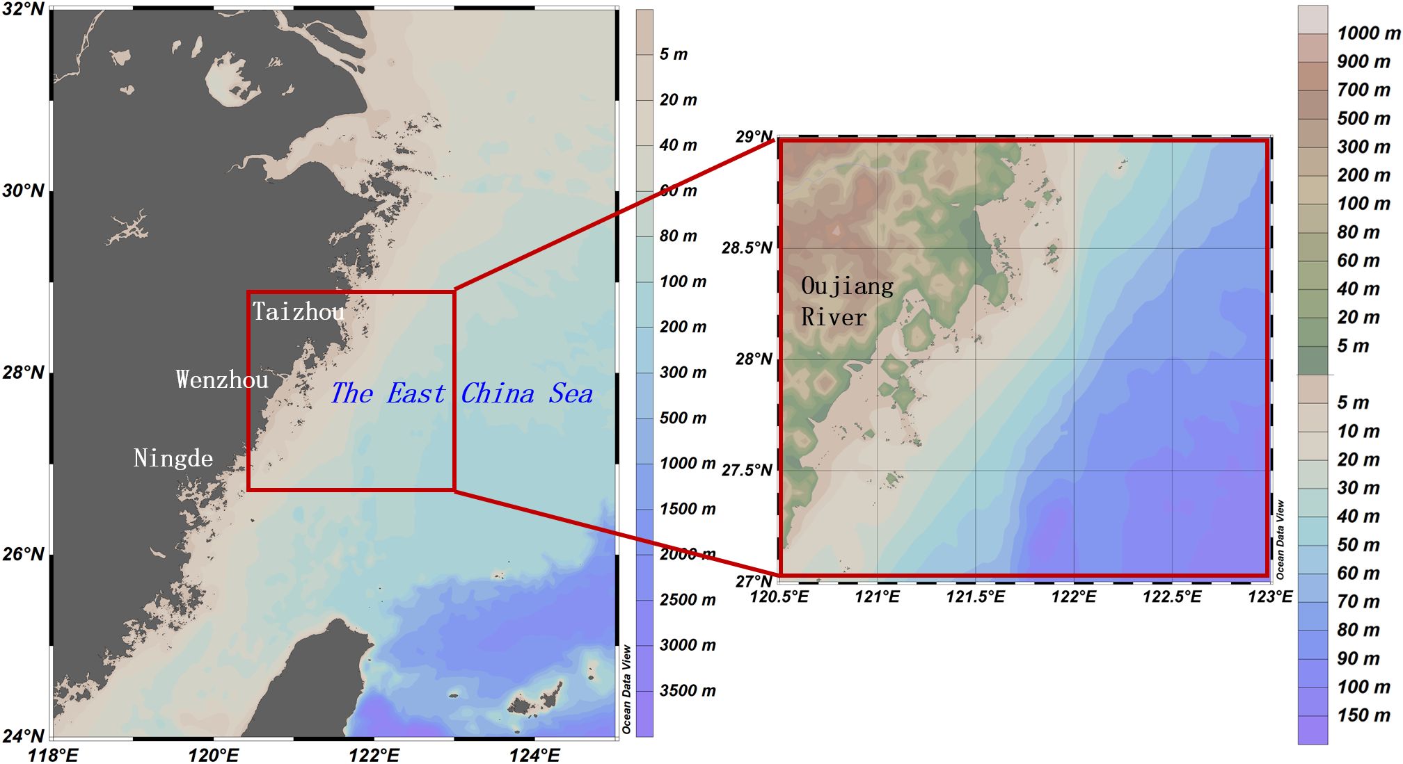
Figure 1 A map showing the study area. The area is distributed near Zhejiang Province, affected by the Yangtze River and Oujiang River.

2.2 Supporting data

In this study, GOCI L2C data were obtained from the KOSC (URL: http://kosc.kiost.ac/) for comparison. A practical atmospheric correction algorithm for turbid waters using ultraviolet wavelengths (UV-AC) (He et al., 2004) was used to retrieve the Remote Sensing Reflectance (R_rs) data first, and then the Chl a, Total Suspended Particulate Matter (TPM) data, and spectral indices (RI₁, RI₂, RI₃) were obtained. The UV-AC atmospheric correction based on the assumption that the water-leaving radiance at ultraviolet wavelengths could be neglected compared with longer wavelengths, and it was suggested quite promising because its performance has been validated in the Changjiang River Estuary with strong spatial and temporal variability of both Chromophoric Dissolved Organic Matter (CDOM) and detritus absorptions (Tzortziou et al., 2008; He et al., 2012). Finally, the HAB information (expressed by RI_i) from 2011 to 2020 was extracted by setting TPM and RI₁ thresholds. This study mainly used remote sensing data from April to September during this decade. A total of 3896 images (410 days) were observed, and 30 pairs of continuous data (the data obtained on June 15–17, 2018 can be regarded as two continuous pairs) were used for analysis in this paper.

Temperature is an important environmental factor for algal bloom occurrence, and it directly or indirectly controls the growth and proliferation of algal bloom organisms. Information on sea surface temperature (SST) data was obtained from the Operational Sea Surface Temperature and Sea Ice Analysis (OSTIA) system (Good et al., 2020), which was developed at the Met Office (https://www.metoffice.gov.uk/). The data used were from a mixture of sources, including in situ data (observed by drifting and moored buoy platforms and ships) and remote sensing data (from satellite SST data), which were distributed through the WMO GTS. Information on salinity, mixed layer thickness, and ocean current velocity was obtained from the GLORYS12V1 product (https://resources.marine.copernicus.eu/). The CMEMS global ocean eddy-resolving reanalysis products have a 1/12° horizontal resolution and 50 vertical levels (Le Traon et al., 2019). Moreover, the regional biases of sea surface salinity (SSS hereafter) were less than 0.2 psu.

2.3 Records of harmful algal bloom events

There were 69 HAB data points collected in the HAB bulletin of Zhejiang Province from 2011 to 2020. Then, according to the matching results of remote sensing data, 32 well-matched cases were selected for analysis based on the screened results of remote sensing data. The details for some HAB cases that appeared near Wenzhou and Taizhou cities (prefecture-level cities of Zhejiang Province) from 2011 to 2020 are listed in Table 1. The collected tracking dataset included the HAB position, intensity, dominant species, and maximum area. According to the records, the duration of these events ranged from 5 days to 24 days. The dominant algae mostly include Karenia mikimotoi and Prorocentrum donghaiense, although there were occasional outbreaks of multi species of phytoplankton (recorded in 2017).

Table 1

Table 1 HABs that affected the coastal waters of Zhejiang provinces from 2011 to 2020.

Since an extensive HAB monitoring network was established in 2000 (Wang and Wu, 2009), annual reports on HAB occurrence have been issued by the Ministry of Natural Resources of the People’s Republic of China (https://www.mnr.gov.cn//sj/sjfw/hy/gbgg/zghyzhgb/). Reports on HAB occurrence (timing, location, intensity) in the ECS have also been obtained from other public data sources, such as the Department of Natural Resources of Zhejiang Province (https://zrzyt.zj.gov.cn/). From these reports, the records we used were found along the Zhejiang coast between 2011 and 2020. The records included the location, start time, end time, areal extent, and species, which were used as the ground truth data to validate HAB delineation on GOCI imagery.

3 Methodology

3.1 Data processing

The study of the correlation between Chl a time series and dynamic changes in HABs based on remote sensing mostly consists of three steps: GOCI image data processing, product generation, and HAB growth prediction (Figure 2). Three different color boxes frame the details of the three steps. Figure 2 was based on the process of the RI₁ (Li et al., 2020) selected in this paper. The UV-AC algorithm was used in the first step. He et al. (2012) discovered that, through analyzing in situ spectra from major water bodies such as the Yangtze River estuary and the Mississippi River, the concentration of Total Suspended Matter (TSM) in China’s coastal waters is relatively high. This causes strong scattering of particles in the water, leading to an increased water-leaving reflectance in the Visible Light (VIS) long wavebands and Near Infrared (NIR) bands. However, the strong absorption of CDOM in the UV spectrum results in a low water-leaving reflectance. Consequently, the UV range is more suitable for atmospheric correction than the NIR range, thus the UV method is recommended. In previous research, the UV method was successfully applied to the GOCI (Qiao et al., 2021). Since GOCI does not possess a UV band, the 412nm wavelength was selected as the reference band. The specific UV-AC algorithm procedure comes from the paper written by Qiao et al. (2021); Qiao et al. (2024).

Figure 2

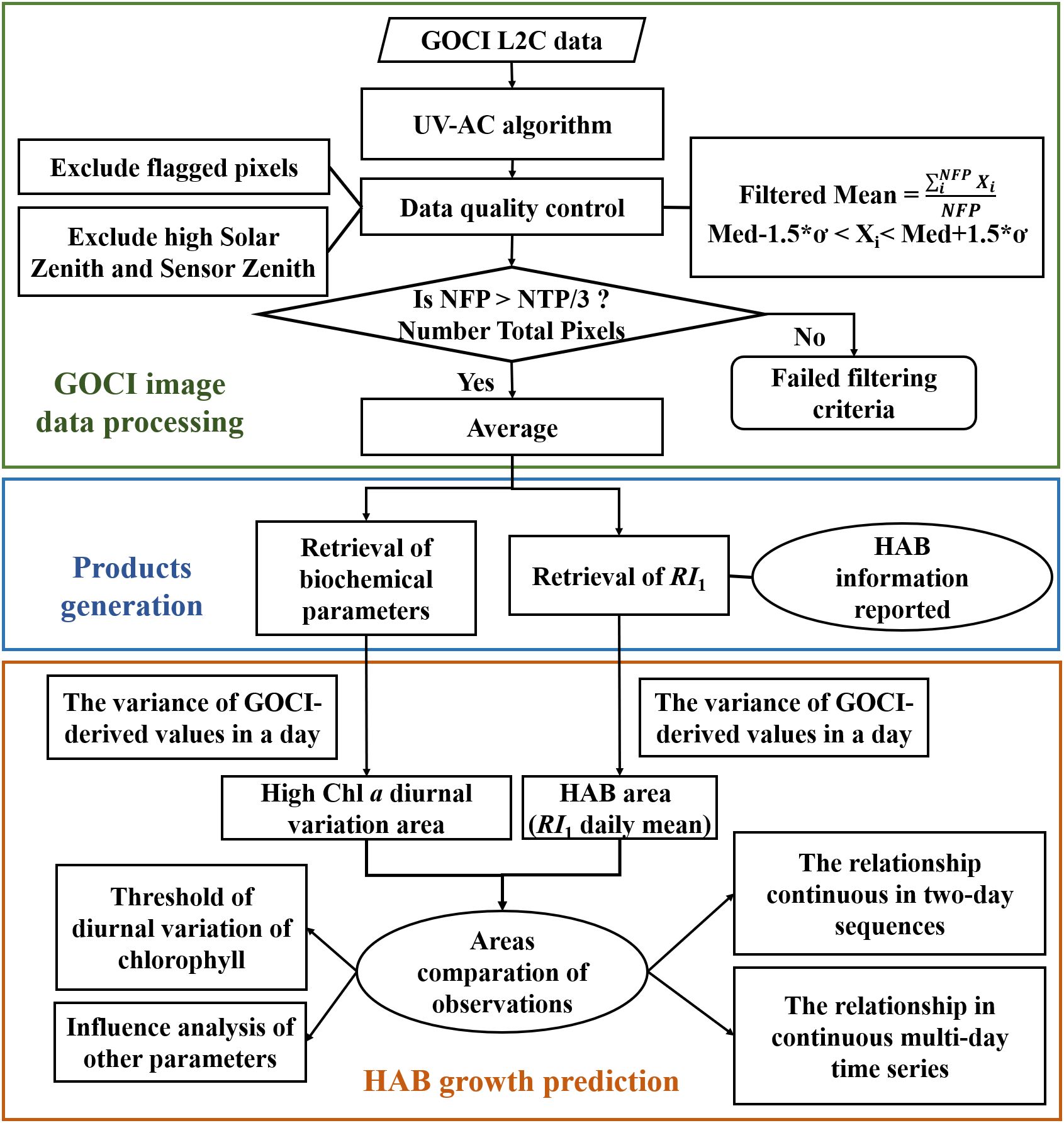
Figure 2 Diagram illustrating the workflow. It mostly includes three modules: GOCI image data processing (green box), product generation (blue box), and HAB growth prediction (red box). The detailed steps of each module are described in different boxes.

In the process of GOCI image data processing, it is necessary to screen the satellite remote sensing data with stringent criteria (Siswanto et al., 2011; Nazeer et al., 2020). In terms of time, the satellite data acquisition time needed to be consistent with the HAB growth time; in space, each target pixel of the remote sensing product was taken as the center, and the observed values of the pixels in the 3×3 window were selected for matching calculation. A pixel was rendered invalid for the matching analysis when it encountered one of the following criteria: a negative R_rs value, land, clouds, a high satellite zenith angle (>60°), or a high solar zenith angle (>75°). R_rs values outside the maximum limit (Equation 2) were also discarded, which means that R_rs needs to meet the following Equation (1) (Concha et al., 2019):

$\begin{array}{ll}(Med-1.5\sigma )<X_i<(Med+1.5\sigma )& (1)\end{array}$

where $X_i$ is the ith filtered pixel in the 3×3 array, Med and σ are the median value and the standard deviation of pixels that satisfied screening criterion mentioned before in the 3×3 array, respectively.

Then, if the number of effective pixels was greater than 1/3 of the total pixels in the window (Nazeer et al., 2020), the mean of the window was calculated as the matching value of the target pixel.

Many spectral indices have been developed to identify algal blooms. Therefore, we use three frequently used indexes (Lou and Hu, 2014; Li et al., 2020; Shen et al., 2019) in this paper, all of which were proposed based on the HAB events along the coastal waters of Southeast China. After the most suitable spectral index was selected, HAB products (expressed as RI_i) and Chl a products were obtained. Here, we calculated the diurnal variation in chlorophyll a: the standard deviation calculated from the daily GOCI-derived chlorophyll a observations. In the process of HAB growth prediction, we mostly analyzed two observed objects (high Chl a diurnal variation area; HAB area), and the area where Chl a diurnal variation was greater than 2.2 mg/m³ was defined as the high Chl a diurnal variation area (the selection methods and standards of thresholds are described in Section 5.2). We also analyzed the correlation between two observed objects in continuous two-day/multiday sequences. Finally, the long-term variation in HAB and the influence of other parameters were discussed.

3.2 Ocean-color algorithms

Many scholars have used satellite-derived Chl a data to describe the spatial extent of HABs. However, although various regionalized Chl a algorithms have been developed, the current algorithm used to retrieve Chl a products is still based on the high absorption of Chl a at the blue band, which often shows high uncertainties in coastal waters because of the high suspended sediments and/or colored dissolved organic matter (Dai et al., 2022; Kim et al., 2016). Moreover, HABs caused by algae with low cellular Chl a content are not easily detectable (Cokacar et al., 2004), and harmless algal blooms may result in a high Chl a signature, making it impossible to distinguish HABs from non-HABs. Therefore, this paper does not analyze the above methods.

Related studies show that suspended sediment can affect the phytoplankton community structure of coastal water, together with nutrients. The high concentration of TPM will inhibit the outbreak of HAB, and the water with high TPM will appear with strong reflection in the infrared band and near-infrared band, which will affect the accurate extraction of HAB in the coastal water. Therefore, when extracting the HAB area, Li et al. (2020) set the thresholds of TPM and RI₁ in the coastal waters of Zhejiang Province to 17 mg/L and 0.23, respectively. The calculation formula is the Equation 2.

$\begin{array}{ll}R{I}_1= \frac{Rrs\left(555\right)-Rrs\left(490\right)}{Rrs\left(555\right)+Rrs\left(490\right)};\text{ Threshold }0.23& (2)\end{array}$

Coastal waters are characterized by high turbidity caused by suspended matter originating from resuspension of sediments, coastal erosion, and river discharge (NeChad et al., 2010). He et al. (2013) proposed a TPM algorithm based on GOCI data in Zhejiang coastal sea areas. The error is small when comparing the five typical algal bloom events in 2011 and 2016 with the algal blooms area detected by the RI₁. It was an empirical algorithm as shown in Equation (3), and R was calculated by Equation (4).

$\begin{array}{ll}TPM= {10}^{1.0578+1.1230\times R}& (3)\end{array}$

$\begin{array}{ll}R= \frac{Rrs(745)}{Rrs(490)}& (4)\end{array}$

Suppressing the effect of resuspended sediments by subtracting the R_rs(443) in the green to blue band ratio, the RI₂ reported by Lou and Hu (2014) performed well for bloom detection in the ECS. The RI₂ threshold is selected to be 2.8 for its application, and a higher value implies a higher density of the bloom. The case study showed that using GOCI data and a modified RI₂ approach appears effective in delineating surface bloom patches in the sediment-rich coastal waters off Zhejiang coast in the ECS. The specific calculation is shown in the following Equation (5).

$\begin{array}{ll}R{I}_2= \frac{Rrs\left(555\right)-Rrs\left(443\right)}{Rrs\left(490\right)-Rrs\left(443\right)};\text{ Threshold }2.8& (5)\end{array}$

The mathematical relationship of the three-band blended reflectance and Chl a can mostly be regionally specific and uncertain due to the algal diversity and the difference in water types. To simplify practical operations, Shen et al. (2019) followed the concept of the three-band model and defined RI₃ for the detection of algal blooms. The results indicated that the RI₃ is effective in detecting algal blooms when using GOCI data, through verification using in situ investigations and cross-comparisons with the multi-source data. The specific calculation is shown in the following Equation (6).

$\begin{array}{ll}R{I}_3=\left(\frac{1}{Rrs\left(660\right)}-\frac{1}{Rrs\left(555\right)}\right)\times Rrs\left(745\right);\text{ Threshold }0.15& (6)\end{array}$

Chl a is an important parameter that we studied. Kim et al. (2016) adjusted the coefficients of the Tassan (1994) algorithm (Tang et al., 2004) according to different water turbidity. The results showed that the absolute percent difference (APD) of Tassan (MS) designed for a TPM concentration of 0.5–10 g/m³ can reach 35%, the relative percent difference (RPD) is within ±2%, and the correlation coefficient is approximately 0.8 The calculation is shown in Equation (7) and Equation (8) below.

$\begin{array}{ll}Chl a={10}^{f_0+f_1\times lo{g}_{10}R+f_2\times lo{g}_{10}{R}^2}& (7)\end{array}$

$\begin{array}{ll}R=(\frac{Rrs(443)}{Rrs(555)}){(\frac{Rrs(412)}{Rrs(490)})}^{f_3}& (8)\end{array}$

$$f_0=0.1235; f_1=-1.6072;f_2=4.6815; f_3=-1.0138$$

Based on an extensive in situ bio-optical dataset, several algal bloom indices were proposed, which are related to the absorption characteristics of HABs. In our study, the UV-AC algorithm was used to process GOCI-L2C data, and then HAB could be identified by Li et al. (2020) index. The further reasons for choosing these index were discussed in Section 5.2.

4 Results

4.1 The relation between HABs and diurnal variation of Chl a

Here, statistical analysis on two-day pairs (three consecutive days of data can be regarded as two pairs of two-day sequences) and multiday sequences was performed to test whether the diurnal variation in chlorophyll a can help to predict the growth state of HABs. In this paper, we extracted 32 pairs of two-day sequences, of which 30 pairs showed that the Chl a diurnal variation retrieved by remote sensing had a certain correlation with the development and disappearance of HAB. Then, the consecutive multiday data were monitored and analyzed, and some special conclusions were obtained.

Table 2 shows the changes in the high Chl a diurnal variation area and HAB area along the coast of Zhejiang Province. Taking two consecutive days as a group, the change trend of the high Chl a diurnal variation area was consistent with that of the HAB area. When the high Chl a diurnal variation area increased, the HAB area also increased. Therefore, we think that the trend of high Chl a diurnal variation areas may help to predict the growth state of HAB.

Table 2

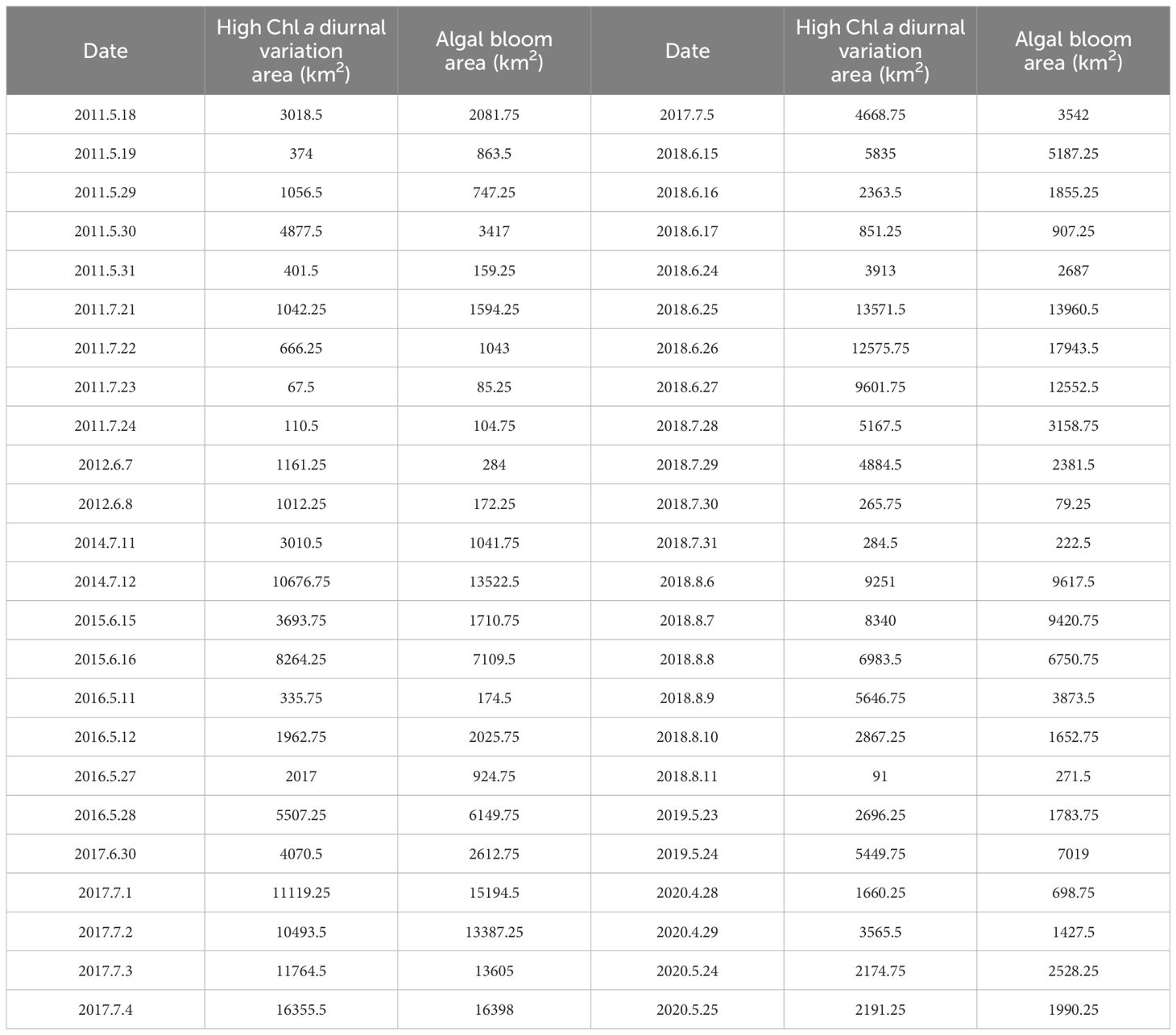
Table 2 Statistical results of high Chl a diurnal variation area and algal bloom area along the coast in areas near Zhejiang province.

Then, we explored the relationship between the high Chl a diurnal variation areas and HAB areas in all continuous time series (Figure 3). The abscissa in Figure 3 shows the initial and end dates of each group of continuous time series, and the time span of the series ranged from 2 days to 6 days. Except that the change trend of the high Chl a diurnal variation area was basically consistent with that of the HAB area, Figure 3 also showed that when the high Chl a diurnal variation area was larger than the HAB area, the HAB area would increase in the next day in most cases. In contrast, the HAB area may decrease accordingly. For example, on July 11, 2014, June 15, 2015, and June 30, 2017, the high Chl a diurnal variation area was larger than HAB area, and the area of HAB expanded significantly the next day, while on June 30, 2017 and June 26, 2018, the HAB area decreased the subsequent day. However, from July 28 to July 31, 2018, the high Chl a diurnal variation area decreased day-to-day, although the high Chl a diurnal variation area was larger than that of HAB. At this time, it may have been in the HAB disappearance period, and the high Chl a diurnal variation area and HAB area changed with the growth state of HAB.

Figure 3

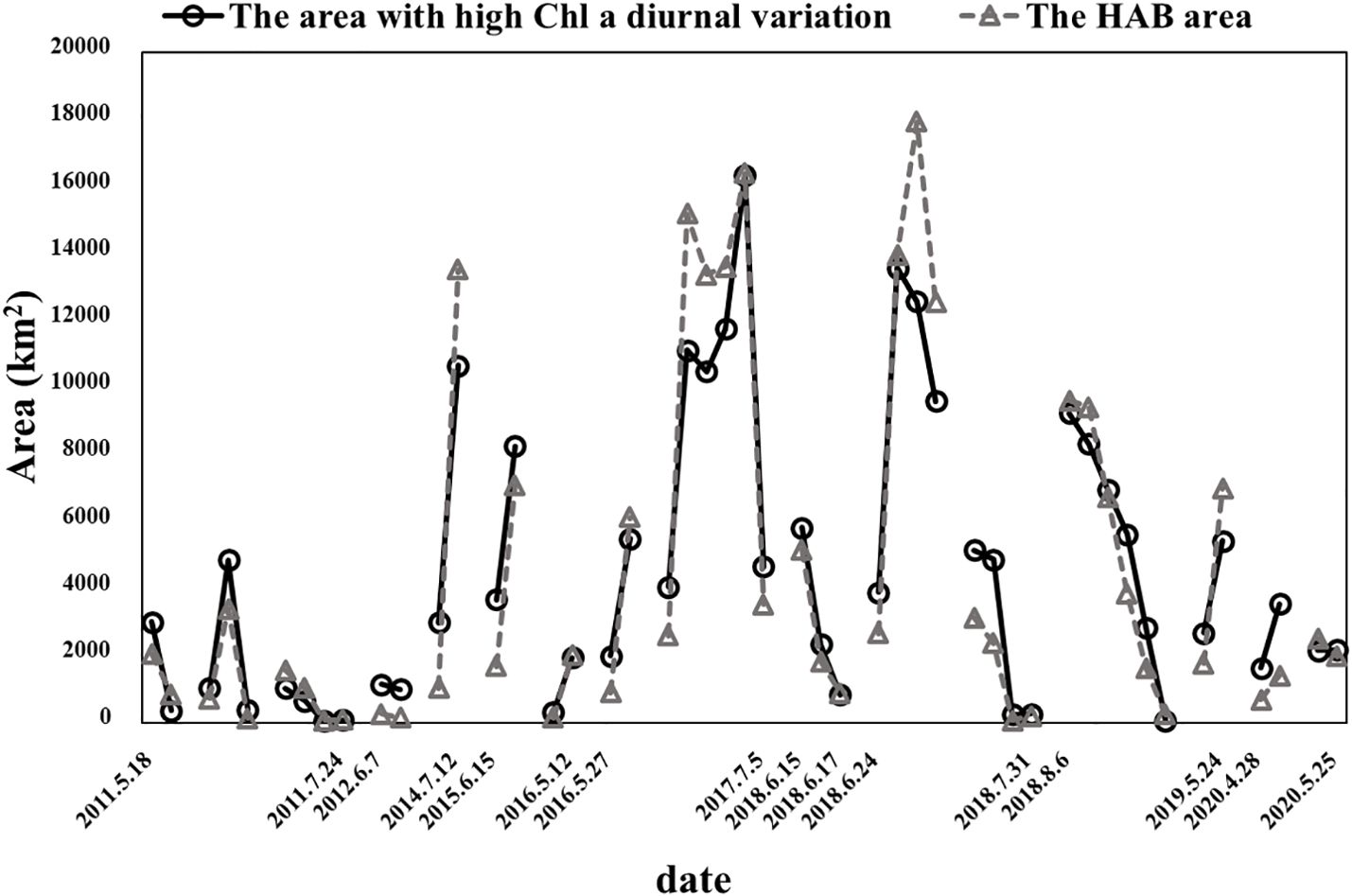
Figure 3 Changes in the high Chl a diurnal variation area and HAB area in all continuous time series. The abscissa shows the start and end dates of each continuous time series. The solid line represents the change in the high Chl a diurnal variation area, and the dotted line represents the change in the HAB area.

4.2 Changes in the spatial distribution between the HAB and chlorophyll a sequence

4.2.1 Continuous two-day sequences

For mapping and spatial analysis, we visualized the observed results from consecutive remote sensing images. Figures 4, 5 show the two-day HAB areas in different colors, and the high Chl a diurnal variation area (greater than 2.2 mg/m³) for the day before in the two-day sequence derived from GOCI was outlined by blue closed curves. The changes in the bloom spatial patterns in inshore waters were represented by high spectral index values (RI₁> 0.23, orange and red colors on the images). From the comparative results of the two observed datasets, the diurnal variation in Chl a could indicate whether the HAB broke out or receded the next day to some extent. When it was found that the HAB area coincided with the high Chl a diurnal variation area or when there was a lower diurnal variation in the HAB area, such as the results that appeared on June 15–17, 2018, the HAB area did not increase or even decreased the next day. However, if the two observed areas were different, a new HAB may have occurred the next day in areas where chlorophyll a had a high diurnal variation but no HAB was detected, as in the case of June 15–16, 2015.

Figure 4

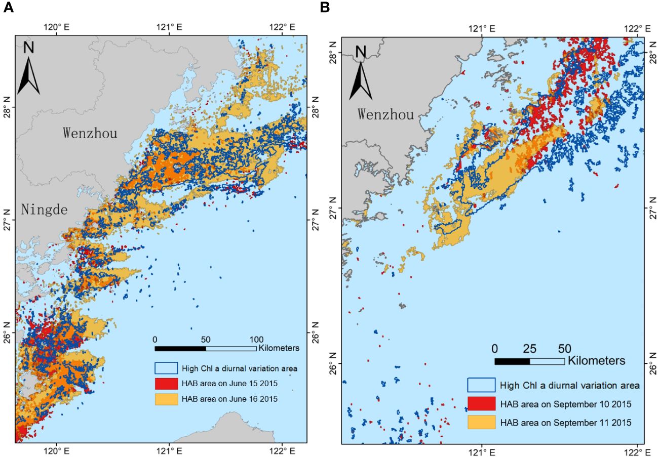
Figure 4 Some results of HAB in 2015. The two subimages show the changes in HAB areas and high Chl a diurnal variation areas along the coast of southern Zhejiang and northern Fujian (A) from June 15 to 16, 2015, and (B) from September 10 to 11, 2015. The area surrounded by dark blue lines is the area where the diurnal variation in Chl a is more than 2.2 mg/m³, the red area is the area where HAB was detected, and the orange area is the area where HAB was detected the next day.

Figure 5

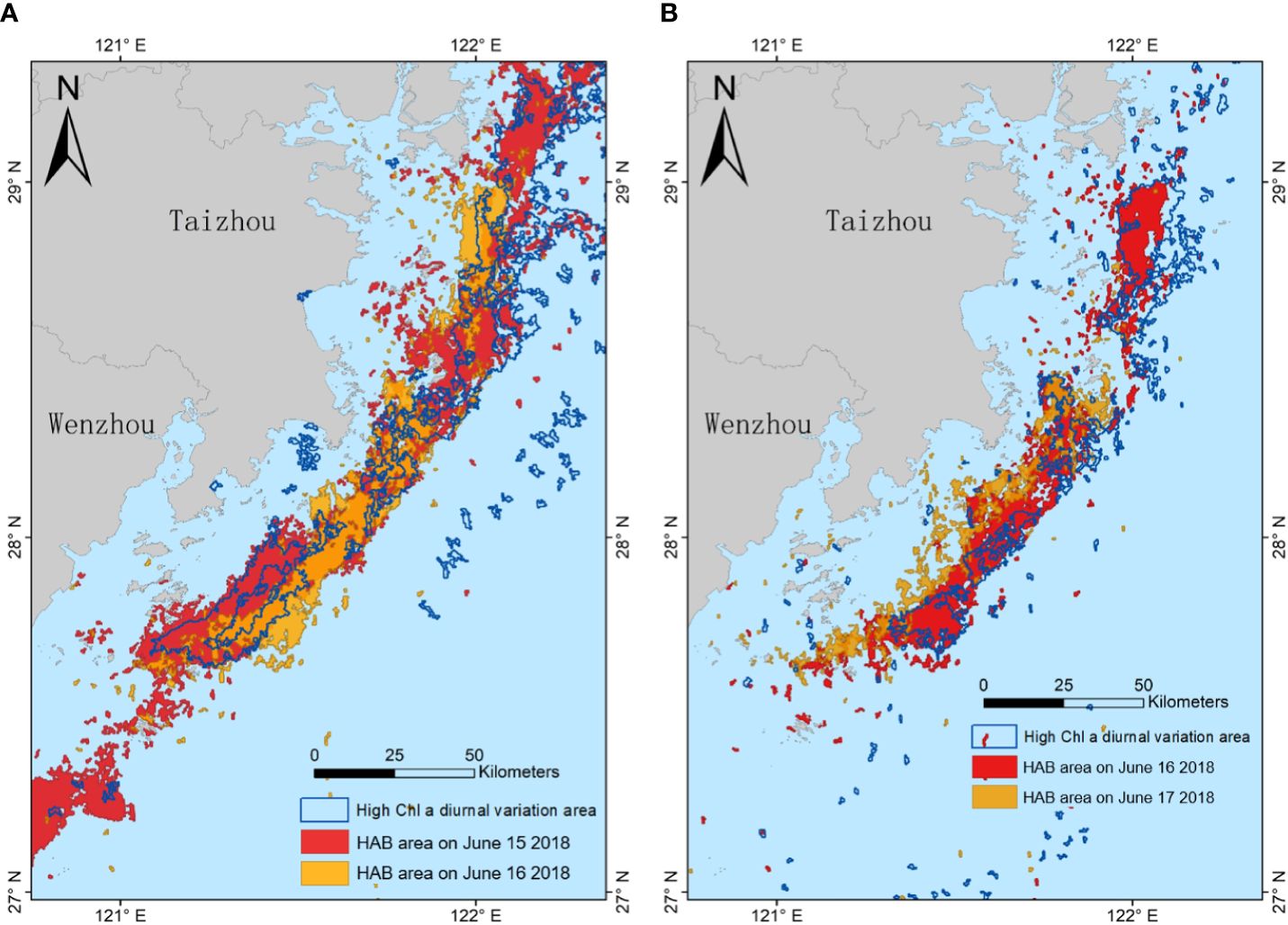
Figure 5 Some results of HAB in 2018. The two subimages show the changes in HAB areas and high Chl a diurnal variation areas along the coast of southern Zhejiang (A) from June 15 to 16, 2018, and (B) from June 16 to 17, 2018. The area surrounded by dark blue lines is the area where the diurnal variation in Chl a is more than 2.2 mg/m³, the red area is the area where HAB is detected, and the orange area is the area where HAB is detected the next day.

From the HAB cases shown in Figure 4, there were some dynamic changes in the results of HABs. From June 12 to June 21, 2015, HABs dominated by Gonyaulax polygramma broke out in the coastal waters of Zhejiang Province. Figure 4A shows the satellite-observed spatial distribution of HABs in the study areas. On June 15, 2015, the area of HAB detected was small (the red area in Figure 4A), while the high Chl a diurnal variation area was larger. Then, a larger HAB area was detected in the high Chl a diurnal variation area on June 16 (the orange area in Figure 4A). The period from June 15 to 16 was in the prophase of the whole HAB life cycle, during which the nutrients in the study area were likely to be rich. Therefore, the high diurnal variation in Chl a was larger, and the HAB area also increased. This phenomenon was particularly obvious along the coast of Wenzhou. On June 16, 2015, a large area of HAB broke out in and around the areas with high Chl a diurnal variation.

Similarly, the same observation was obtained in the images from September 10 to 11, 2015. HABs dominated by Phaeocystis globosa broke out in the ECS from September 10 to 19, 2015. From the images, the total HAB areas detected in the two-day sequence were smaller than those in June 2015, especially in the waters of eastern Wenzhou. Most of the areas along the coast of Wenzhou and Ningde showed multipoint HAB outbreaks on September 10, while a massive HAB area was detected the next day.

Several HABs broke out along the coast of Zhejiang Province in June 2018, and the dominant algae were mostly composed of Prorocentrum donghaiense and Karenia mikimotoi. Many remote sensing images were available for analysis in that year, as shown in Figure 5. From June 15 to 17, 2018, the outbreak areas of HAB in the first two-day sequence were generally smaller than those in the latter group. The HABs in the coastal area were distributed in a strip, and the HAB areas decreased day-to-day. These days, the high Chl a diurnal variation area and the HAB area observed had a high coincidence degree, and the HAB area showed a decreasing trend the next day. The HAB areas in Figure 5 were mainly concentrated along the coasts of Taizhou and Wenzhou cities. In Figure 5B, the HAB area on June 17 was smaller than that of the previous day, and the high Chl a diurnal variation area was also smaller than that of HAB on June 16. Notably, the area of the dark blue boundary line was similar to that of the HAB on June 17 with a slight deviation. It may be the reason for the change of flow field.

4.2.2 Continuous multiday time series

Furthermore, we analyzed several continuous multiday time series (3 consecutive days or more). The results showed that continuous multiday diurnal variation in Chl a could reflect the HAB’s overall growth condition. If the high Chl a diurnal variation area increased gradually over several consecutive days, the HAB areas would also increase on these days; in contrast, the HAB areas would decrease, and it may have been during the period of HAB disappearance.

As shown in Figure 6, from August 7 to August 10, 2018, the high Chl a diurnal variation area in the coastal waters of Taizhou and Wenzhou decreased each day, as did the areas where HAB was detected during this period. On August 8, 2018, the HAB in the waters near the Oujiang River appeared to be larger and stronger than that on August 7. Then, the HAB area declined rapidly on August 9. From August 7, 2018 to August 10, 2018, the diurnal variation in Chl a in the sea area between 27.6°N to 28°N and 120.5°E to 121°E continued to be high, as did the Chl a diurnal variation in the area between 28.3°N to 29°N and 122°E to 122.5°E. Scattered HAB points could still be detected in these two areas on August 10 (when the HAB basically disappeared).

Figure 6

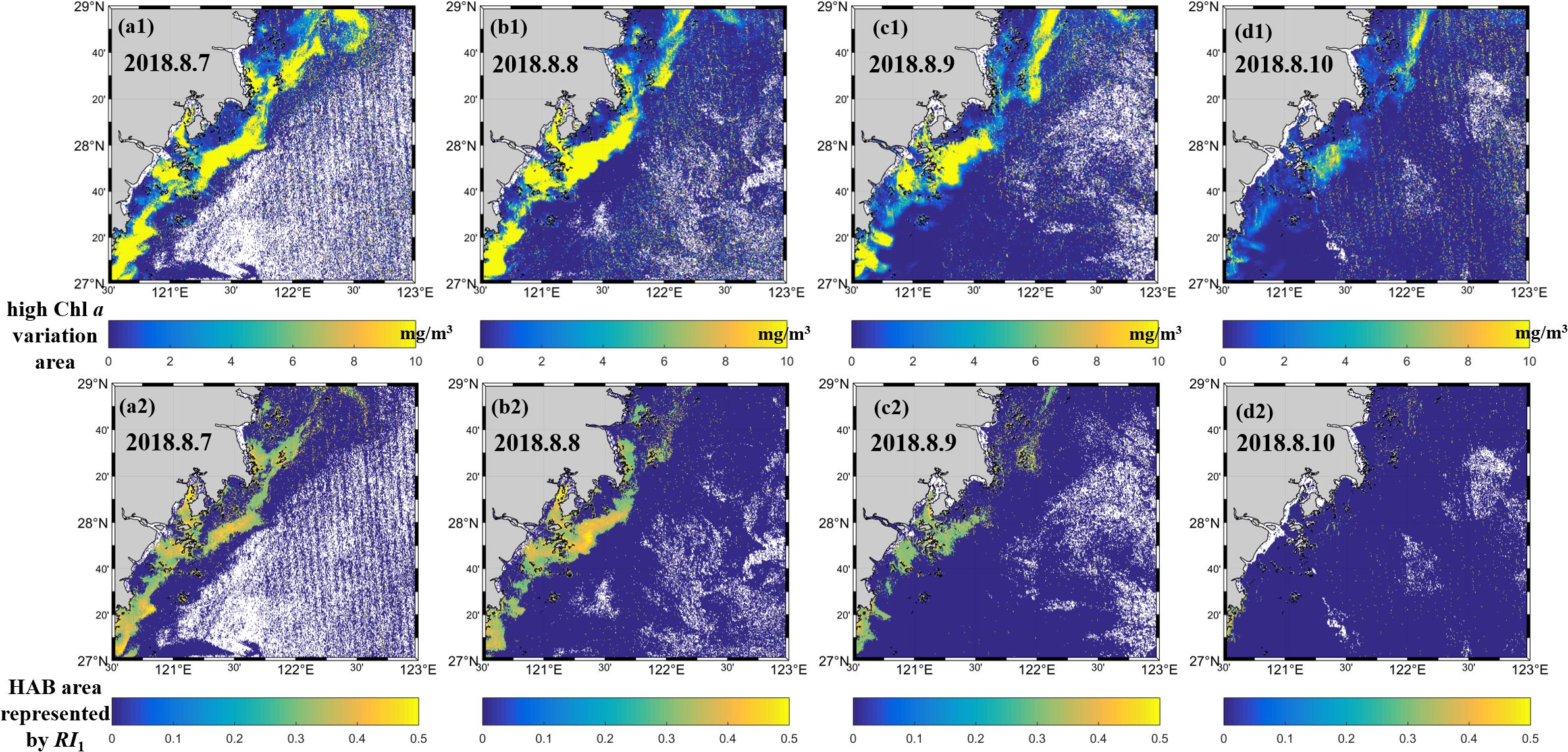
Figure 6 Some results of Chl a and HAB on (a) August 7, 2018; (b) August 8, 2018; (c) August 9, 2018; (d) August 10, 2018. The submap with suffix 1 is the area with high Chl a variation, and the submap with suffix 2 is the HAB result represented by RI₁.

From Figures 6(a1), (a2), (b2), the high Chl a diurnal variation area on August 7, 2018 was slightly larger than the area where the HAB was detected, especially in the sea area between 28.5°N to 29°N and 122°E to 122.6°E, but the HAB area detected in this area did not increase on August 8. However, from the results of continuous multiday time series, the high Chl a diurnal variation area continued to decrease, and the HAB was in a state of gradual disappearance, so this phenomenon was still reasonable.

Table 3 shows some statistical results (median RI₁ and 90% median line of Chl a concentration) in the area near Zhejiang Province. The median results can avoid the influence of some extremes on the analysis results, and the 90% median line of Chl a concentration can roughly represent the Chl a concentration in the HAB area, which helps us to understand the state of phytoplankton. The calculated median results of the HAB areas were consistent with the image observation results. The median RI₁s of the HAB area were all in the range of 0.25–0.50. Interestingly, the changing trend of most median RI₁ values corresponded to the development and disappearance of HABs, and the changing trend of the 90% median line of Chl a was also roughly the same. From the satellite image, some HAB breakpoints were often retrieved in offshore waters, which may have affected the calculation results in this paper. The occurrence of breakpoints might be due to the interference caused by the algorithms used in the image processing. Therefore, in the case of the overall disappearance of the HABs (as shown in Figure 6), the median value of the RI₁ calculated on August 11 was larger than that of the previous days, which may have been mainly affected by the above interference.

Table 3

Table 3 Statistical results in areas near Taizhou and Wenzhou cities.

5 Discussion

5.1 The selection of the spectral index and threshold

Since the HAB area retrieved by spectral index is almost larger than the actual area reported by the HAB records, we compared three frequently cited HAB retrieval algorithms and applied one of them. In this paper, the intersection of the HAB area extracted by the three spectral indices was considered the area where the HAB occurred. Figure 7 shows the HAB area extracted from three spectral indices on June 11, 2018. We also show the Chl a concentration map as a comparison to assist the analysis.

Figure 7

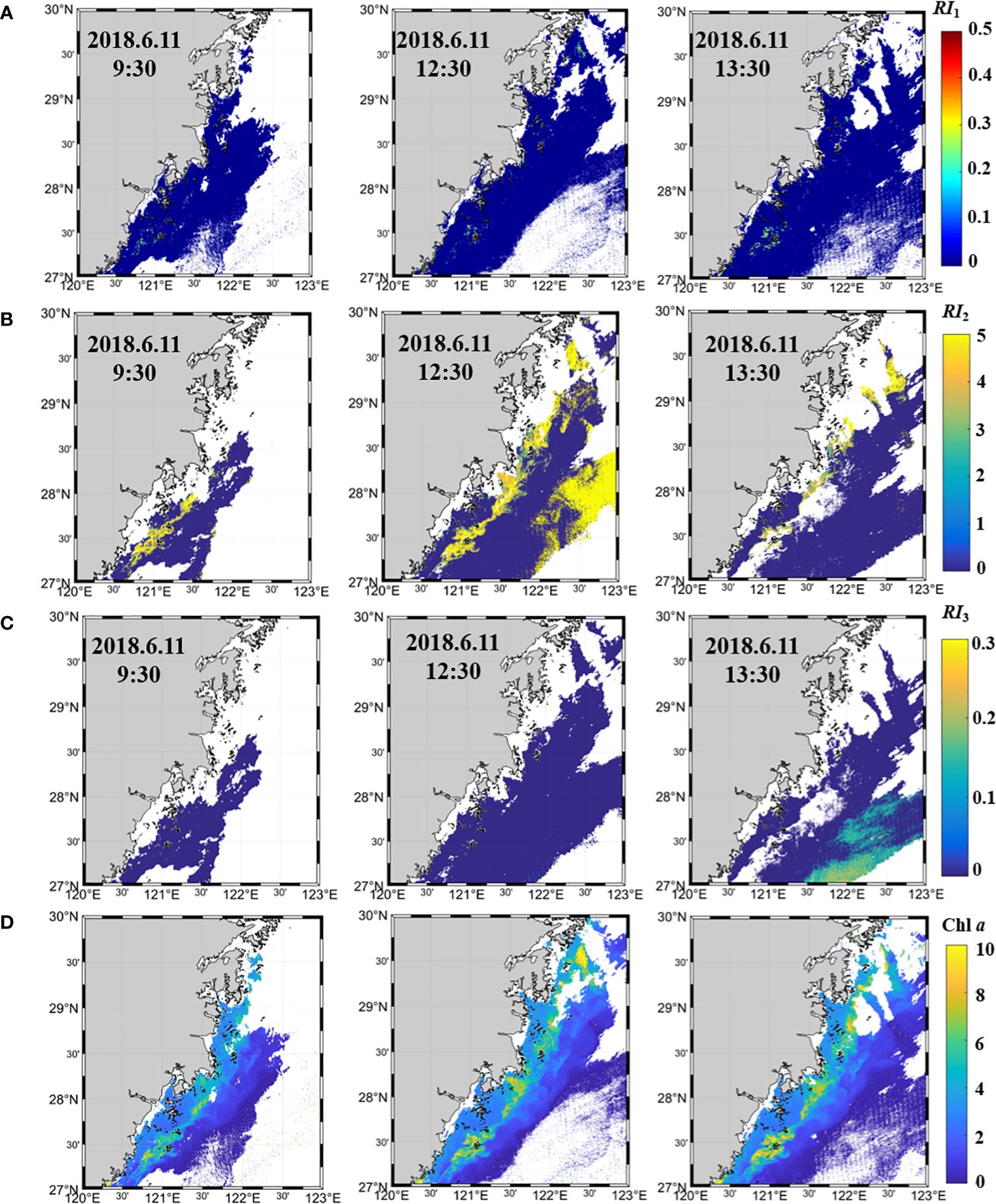
Figure 7 Some results of HAB on June 11, 2018. They were HABs retrieved by (A) Li et al. (2020) index; (B) Lou and Hu (2014) index; and (C) Shen et al. (2019) index, and (D) Chl a.

From the retrieval results of the three algorithms, the HAB area detected by Li et al. (2020) index was smaller than that of the other two algorithms. As shown in Figure 7A, a smaller HAB was detected in the southern part of the coast of Wenzhou, which was slightly pronounced at 12:30 and 13:30. In addition to the larger HAB area detected in coastal water (Figure 7B), it was also detected on the far shore at 11:30 and 12:30. Figure 7C shows that Shen et al. (2019) index could also detect HAB at the far shore. This may be because the atmospheric correction algorithm used was the infrared atmospheric correction algorithm, which is not particularly suitable for coastal water. From the result of Chl a concentration (Figure 7D), the place with high Chl a concentration is not necessarily identified as the area where algae bloom occurs. The results showed that Li et al. (2020) index best met our needs.

5.2 Threshold of diurnal variation in chlorophyll a

The diurnal variation in Chl a will have different results in different regions. In the regions where the nutrients are rich and the proportion of nutrients is suitable, the photosynthesis of phytoplankton is often strong, and the Chl a diurnal variation may be greater. We calculated the Chl a diurnal variation area of the day on which the HAB was detected and the HAB area on the next day, and then calculated the area difference (km²) between the two values. Figure 8 shows the change in the absolute value after calculating the mean (Figure 8A)/median (Figure 8B) of all the area differences (km²) in the case of selecting different threshold values of diurnal variation in Chl a. The range of Chl a diurnal variation in the analysis was 1.5–6 mg/m³, and the interval was 0.1 mg/m³. The results showed that if the threshold was selected from the absolute values of the mean, the diurnal variation threshold of Chl a should be 1.9 mg/m³, and the difference between the two areas was the smallest. If the absolute value of the median value was calculated, the result is shown in Figure 8B (the threshold was 2.2 mg/m³). The results of Figure 8 show that no matter the mean or median of the area difference is calculated, the two result graphs under different thresholds have obvious minimum results. When the diurnal variation of chlorophyll is 1.9–2.3 mg/m³, the mean or median value of the area difference between the high diurnal variation region and the next day HAB region is relatively small. Considering that the mean value of area difference may be greatly affected by special values such as maximum/minimum, we think that the threshold that can obtain the minimum of the median value of area difference can be regarded as the most appropriate threshold, and we chose the threshold of diurnal variation in Chl a to be 2.2 mg/m³.

Figure 8

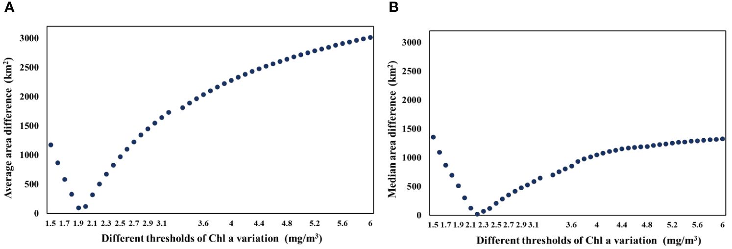
Figure 8 Differences in different thresholds. The threshold is selected from the difference between the high Chl a diurnal variation area and the HAB area the next day, and different results are by calculating the absolute value of (A) average/(B) median.

In this paper, the area differences between two observed objects in consecutive two-day sequences were compared. “Area_difference(%)” was expressed as the difference between the previous day’s high Chl a diurnal variation area and the next day’s HAB area divided by the percentage of high Chl a variation area. The specific calculation is shown in the following Equation (9).

$\begin{array}{ll}{\text{Area}}_{\text{difference}}(\%)=\frac{{\text{Area}}_{\text{day}2\text{ HAB}}-{\text{Area}}_{\text{day}1\text{ high Chl a diurnal variation}}}{{\text{Area}}_{\text{day}1\text{ high Chl a diurnal variation}}}\times 100(\%)& (9)\end{array}$

${\text{Area}}_{\text{day}2\text{ HAB}}$ represents the next day’s HAB area, and ${\text{Area}}_{\text{day}1\text{ high Chl a diurnal variation}}$ represents the previous day’s high Chl a diurnal variation area.

We calculated the Area_difference(%) near Zhejiang coasts. Taking the median of all the results involved, it could be found that the area difference between the two observed objects was approximately -0.08%.

5.3 Variation in HAB along the coast of Zhejiang

5.3.1 Diurnal variation in HAB along the coast of Zhejiang

The vertical migration of phytoplankton can be divided into active migration and passive migration. Among the organisms causing HAB in the Yangtze River Estuary and its adjacent waters, the most dominant HAB algae are considered to be Prorocentrum donghaiense, Skeletonema costatum and Noctiluca scintillans (Liu et al., 2011). Most of the cases selected in this paper were HAB events caused by the accumulation of Prorocentrum donghaiense and Krorolimus michaeli, both of which are dinoflagellates. These algae have strong ability of autonomous movement and can adjust their position in the water body independently. We extracted the HAB in the sea area near Zhejiang Province on June 15, 2018. Figure 9 shows the 8 RI₁ images derived from hourly GOCI data, which showed spatial patterns and changes in HABs in the coastal waters in a day. It can be seen from Figure 9 that the overall position and the center point of the HAB on 15 June changed over time. That is, in addition to changing with time, the HAB also changed in space.

Figure 9

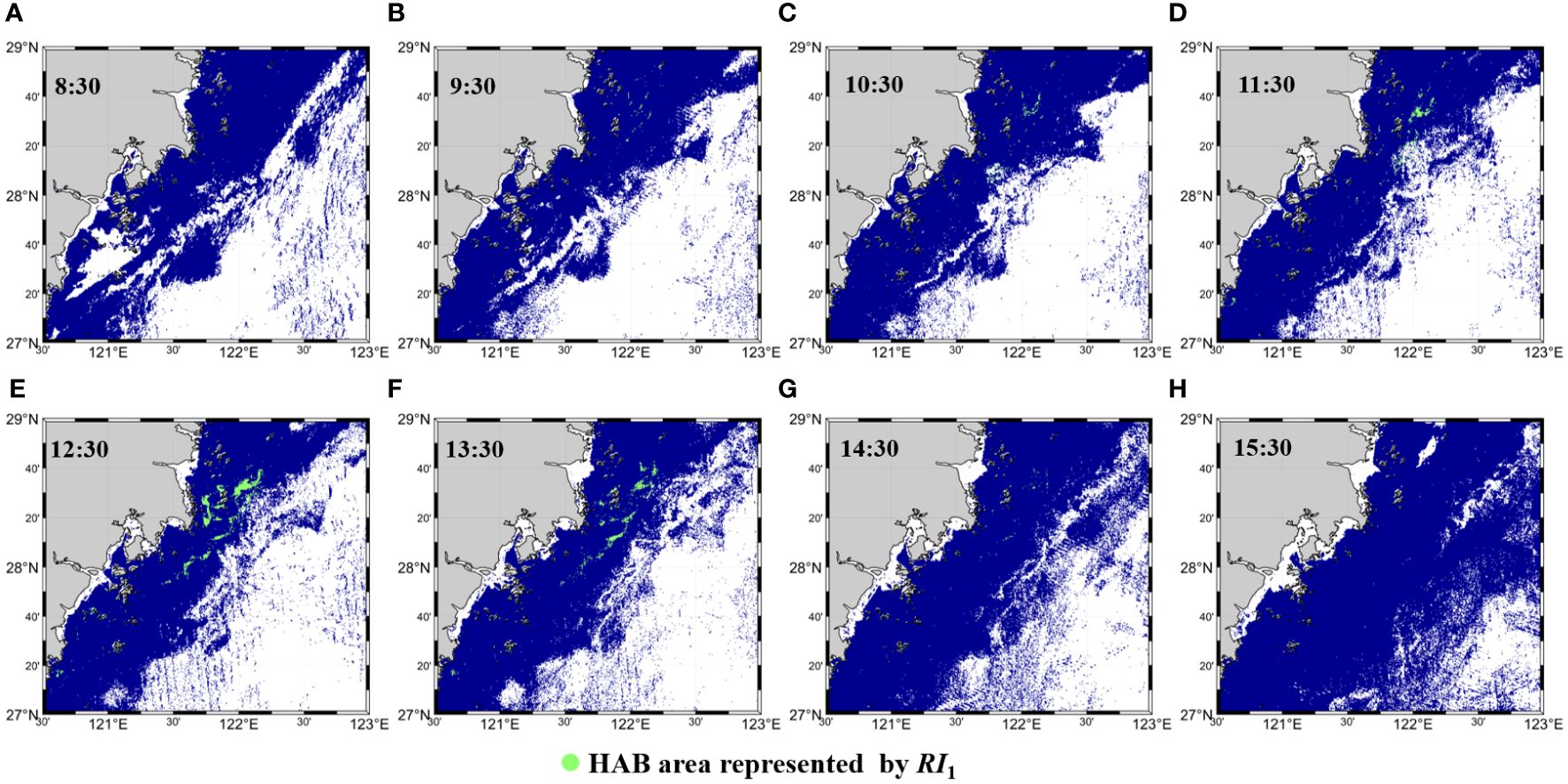
Figure 9 (A–H) RI₁ and Chl a images derived from hourly GOCI data on 15 June 2018. The green area is the extracted HAB areas near Wenzhou and Taizhou cities.

The whole area of HAB first increased and then decreased, which was in accordance with the law of diurnal vertical migration (Lou and Hu, 2014). It appeared that the bloom size always reached a maximum at 13:30 or 14:30. The environmental factors affecting the diurnal distribution and vertical migration of phytoplankton include light intensity, water stratification, water disturbance caused by wind, feeding pressure of zooplankton, individual size of algae, etc. While the changes in bloom size were likely due to the vertical migration of algae, horizontal movement between 8:30 and 15:30 appeared to be driven by physical processes, specifically by tides, which could be important in modulating the initiation, development, and disappearance of HABs.

5.3.2 Long-term variation in HAB along the coast of Zhejiang

Before the HAB breaks out, the population of algae organisms in the sea area has a certain number of individuals. When external conditions such as temperature, salinity, light, and nutrition reach the optimum range for the growth and proliferation of HAB organisms, algae enter the exponential proliferation period and rapidly develop into a HAB (Deng et al., 2009). The HAB growth areas we studied were basically in the Zhejiang coastal area, which is affected by land fresh water. When the Yangtze River, sediment, and nutrients exit the estuary, large portions of them are transported southwards by the coastal current along the inner continental shelf of the ECS, which means that the coastal waters of the ECS are affected by the Yangtze output (Xu et al., 2012; Yang et al., 2023), especially in the Zhejiang coastal area. Eutrophication fueled by riverine runoff of fertilizers will exacerbate primary production in coastal zones. In this paper, we considered that nutrients were closely related to the diurnal variation in Chl a, and from the above results, it was also concluded from the data that the Chl a diurnal variation can predict the next-day growth of HAB.

Figure 10 shows the change in the median GOCI-derived RI₁s along the Zhejiang coast from May to August 2011 to May to August 2020. The reason why the median value is selected as the result is also to reduce the interference of special values. The change in the median GOCI-derived RI₁ in the study area where HAB was detected from 2011 to 2020 showed that the development intensity of HAB fluctuated steadily in these years. Among them, the high value in 2014 mainly occurred in July. Moreover, as shown in Figure 10, we found that the median RI₁ along the coast of Zhejiang showed an increasing trend from May to September (there are relatively few data for April).

Figure 10

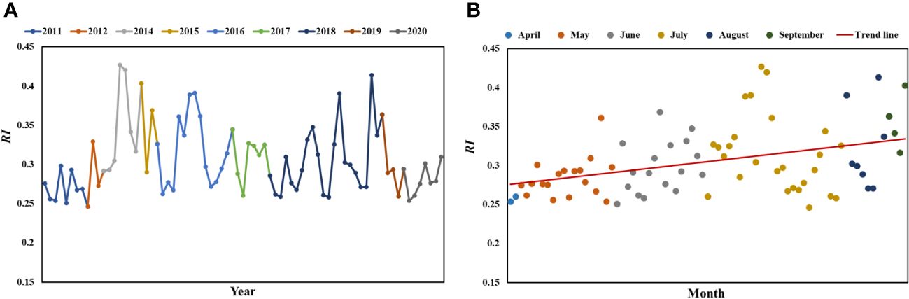
Figure 10 The median RI₁ of HAB detected near Wenzhou and Taizhou cities in GOCI images from 2011 to 2020. (A) The broken lines of different colors represent the results of the median values of HABs retrieved during different years. Among them, all the numerical results are connected by date sorting. (B) Dots of different colors represent the results of different months from April to September. The red straight line indicates the trend line.

5.4 Analysis on the change of other influencing factors

Figure 11 shows the environmental results for some typical days. On June 11, 2018, a weak HAB was detected, and the area of the HAB expanded on June 13, 2018. According to data, typhoon Gaemei passed the northern part of the South China Sea on June 14, 2018, and then made landfall near Taiwan on June 15, which may have impacted this area. The results showed that the coastal currents on June 11 and 15 flowed from north to south, and during this period, the current on June 13 flowed from south to north. From Figure 11A, the area with a deep mixed layer (> 13 m) in the whole region expanded on June 15. According to Figure 5, the HAB area was also large. On June 16, the depth of the mixed layer reached its strongest value, while the HAB area was much smaller than that on June 15. We inferred that the reason for this phenomenon may be nutrient consumption or the increase in water turbidity caused by typhoons. From the results of the flow field, the coastal current moving southwards accounted for a large area on June 15 and 16, which may be mixed with some Yangtze River flushing fresh water carrying many nutrients. Then, on June 17, the northwards-moving TWWC became stronger, bringing a large amount of high-temperature and high-salinity water. Figure 11B shows that during this period, phenomena such as heavy precipitation accompanied by typhoons led to a brief cooling of the water, but the water temperature of the area with detected HAB was in a relatively stable range of 24–26°C.

Figure 11

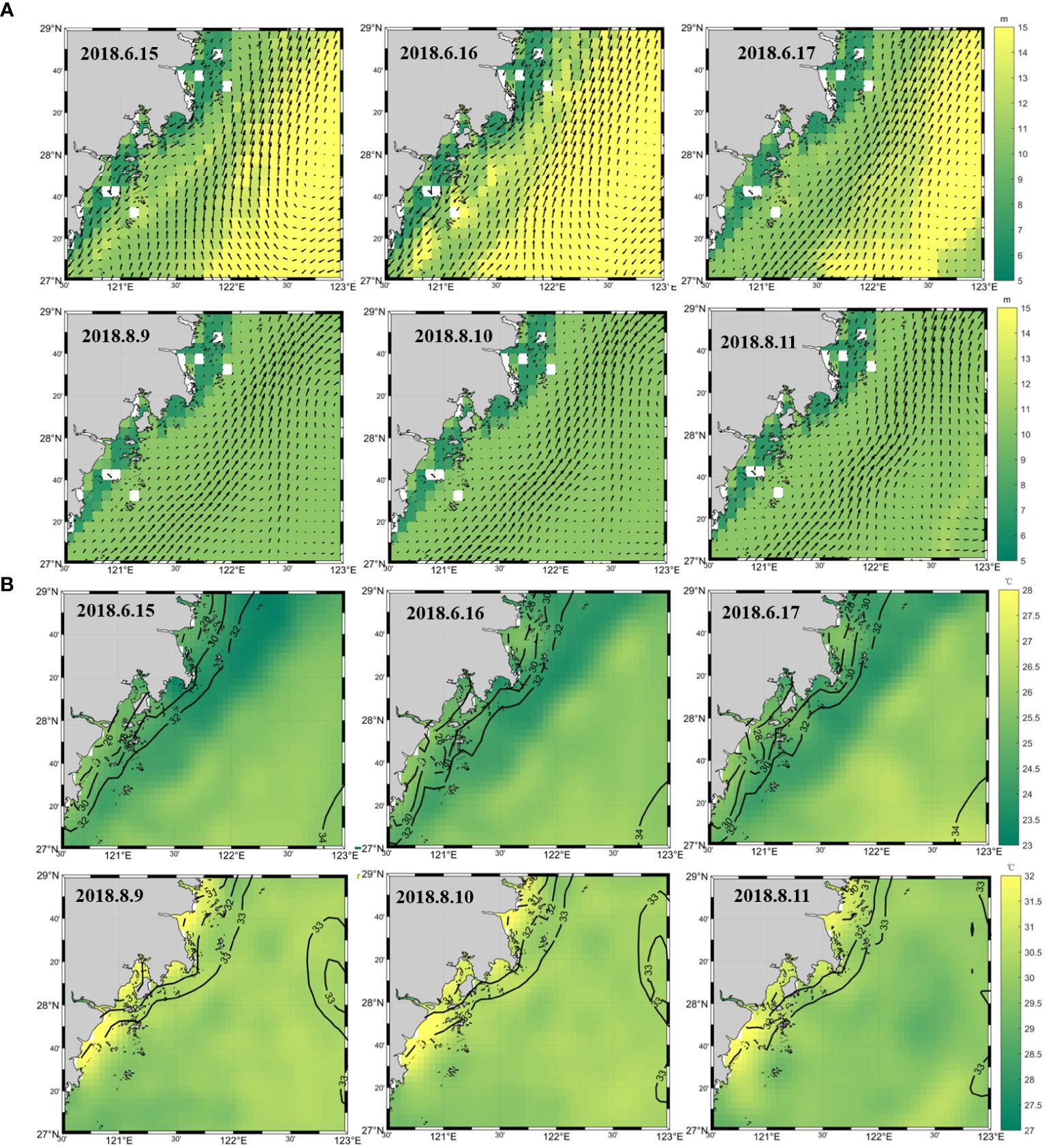
Figure 11 Other environmental factors for several days on the coast of Zhejiang in 2018. (A) Depth of the mixed layer and the flow field. The direction of the arrow indicates the direction of the flow field, while different colors show the depth of the mixed layer of water, ranging from 5 m (green) to 15 m (yellow). (B) Water temperature (unit: °C) and salinity (unit: psu) for several days on the coast of Zhejiang in 2018. Different colors show the water temperature ranging from 23°C (green) to 28°C (yellow) in June and 27°C (green) to 32°C (yellow) in August. Salinity is represented by contour lines.

The surface water in the coastal waters of Zhejiang is mostly affected by the Zhejiang-Fujian coastal current, the Taiwan warm current, the fresh water of the Yangtze River, etc. During June, the image results showed that the Zhejiang-Fujian coastal current was dominated by low temperature and low salinity, while seawater with high temperature and high salinity occupied a large area in August. From August 9 to August 11 2018, the high Chl a diurnal variation area gradually decreased, and the area where HAB was detected also decreased. From the observation results of other environmental conditions in the coastal waters of Zhejiang (Figure 11A), the depth of the mixed layer was almost unchanged, which was approximately 10 meters, and the flow field was mainly controlled by the flow from south to north along the coast. In Figure 11B, the coastal waters of Zhejiang were basically in the range of 30–31°C during this period, and the water temperature changed only slightly. Therefore, we believe that the initiation of HAB is mainly due to external conditions such as temperature and salinity, but the dominant factor affecting the development and disappearance of HAB may be related to nutrients. Combined with Figures 10, 11, we identify that water temperature may be an important factor affecting the intensity of HAB development.

Based on the above results, it can be considered that the previous diurnal variation in Chl a observed from GOCI can help predict HAB dynamics. As shown in Figure 12, solar radiation, flow and nutrients all affect the growth of HABs. Solar radiation and nutrients mainly play a role in biochemistry, and nutrients may come from the Yangtze River flushing fresh water, or from various upwelling. The current physically dissipates or aggregates the algal bloom. The observed areas were categorized as the high Chl a diurnal variation area (A) and the HAB area (B) for comparison. We observed that in the sea area where the diurnal variation in Chl a was high but no HAB was detected, the algae may break out the next day and form a new HAB region. As previously reported, the high diurnal variation in chlorophyll a may reflect that the nutrients in this area were suitable for the mass reproduction of algae. Coupled with suitable temperature and salinity conditions, there was a great possibility for the rapid propagation and growth of algae in this area. However, if the diurnal variation in Chl a was low in the area where the HAB was detected, the HAB in these areas was likely to remain or even disappear the coming day. The nutrients in this area may have been greatly consumed.

Figure 12

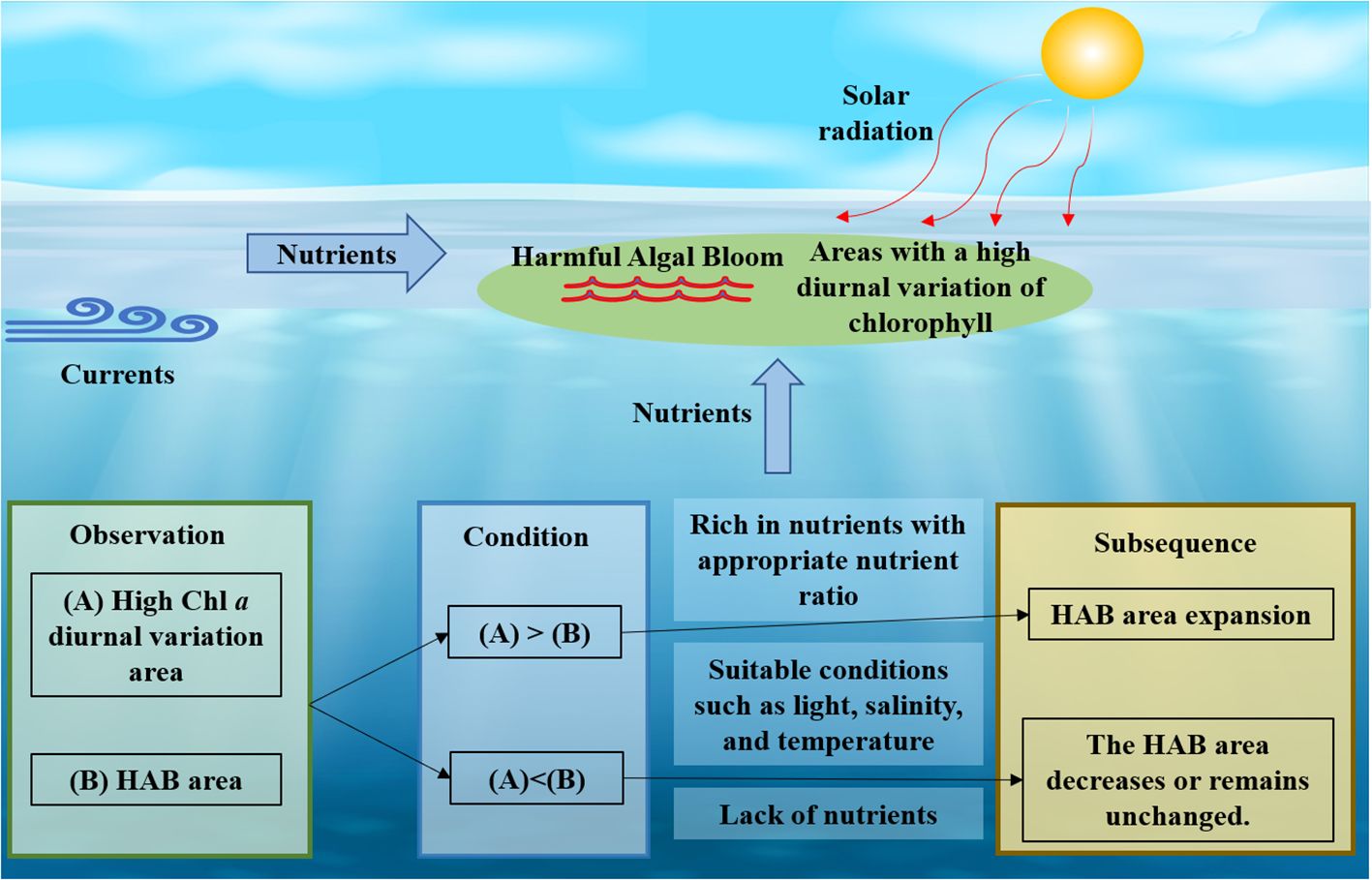
Figure 12 HAB growth analysis and schematic diagram of the study. Rich nutrients with other suitable conditions (light, temperature, and so on) will affect the growth state of HAB. HAB can be predicted by comparing the differences between (A) high Chl a diurnal variation areas and (B) HAB areas.

6 Conclusions

Harmful algal blooms have recently become a serious problem in Chinese coastal waters, causing water quality deterioration. We investigated the applicability of GOCI for monitoring and predicting HAB distributions. The intersection of the HAB area extracted by the frequently cited HAB index was regarded as the remote sensing observed area where the HAB occurred. After comparing the three spectral indices, it is considered that Li et al. (2020) index was more suitable for our needs. In addition, according to the analysis results, the high Chl a diurnal variation in this paper was defined as 2.2 mg/m³. The conclusions drawn from this study are as follows.

From the comparison of the high Chl a diurnal variation area and HAB area, it was found that the diurnal variation in Chl a could be used to predict the spread and growth of HAB the next day. In the observed area where the diurnal variation in Chl a was high but no HAB was detected, the algae may have broken out the sequent day or formed a new HAB region. However, if the area covered by the high diurnal variation is smaller than the area where the HAB breaks out, the HAB in these areas is likely to persist and even decrease the next day.

The multiday observations of the Chl a diurnal variation can reflect the HAB’s overall growth state. The multiday results showed that if the relationship between HAB and Chl a time series does not conform to the above law, it is probably because the time series is in the initiation or disappearance stage of HAB. Then, phytoplankton in the disappearance period of HAB continue to consume nutrients under suitable environmental conditions (when Chl a varies greatly during the day), but there will be no new HAB the next day. The diurnal variation area of Chl a in the disappearance period also decreased day-to-day.

The overall area of HAB agrees with the law of diurnal vertical migration in time, which will first increase and then decrease; in spatial view, there will also be some horizontal movement. We infer that the high Chl a diurnal variation area where the HAB was not detected may have rich nutrients for algae growth, so a new HAB will break out the next day. When the high Chl a diurnal variation area coincided with the HAB area, the nutrients that can be used for growth by these HAB dominant algae in the nearby area may be consumed or can no longer meet the needs of algae growth. Coupled with the comparison of other environmental conditions in the coastal waters of Zhejiang coast, we understand that HAB initiation is mainly due to external conditions such as temperature and salinity, but the dominant factor affecting the development and disappearance of HAB may be nutrients.

Data availability statement

The original contributions presented in the study are included in the article/supplementary material. Further inquiries can be directed to the corresponding author.

Author contributions

YX: Writing – review & editing, Writing – original draft, Investigation, Data curation. JC: Writing – review & editing, Writing – original draft, Funding acquisition. QY: Writing – original draft, Resources. XJ: Writing – review & editing. YF: Writing – review & editing. DP: Writing – review & editing.

Funding

The author(s) declare financial support was received for the research, authorship, and/or publication of this article. This work was supported by the PI Project of Southern Marine Science and Engineering Guangdong Laboratory (Guangzhou) (GML2021GD0809), NSFC‐Zhejiang Joint Fund for the Integration of Industrialization and Informatization (Grant U1609202), National Natural Science Foundation of China (Grants 42076216,41376184 and 40976109), and Funded Program of State Key Laboratory of Satellite Ocean Environment Dynamics (Grant SOEDZZ2203).

Acknowledgments

The authors thank the Korea Institute of Ocean Science & Technology (KIOST) for providing the freely available GOCI data (http://kosc.kiost.ac.kr/), European Space Agency for the information on salinity, mixed layer thickness, and ocean current velocity (GLORYS12V1 product, ftp://anon-ftp.ceda.ac.uk/neodc/esacci/sea_surface_salinity/data/v03.21/), and Met Office for information on sea surface temperature (SST) data (Operational Sea Surface Temperature and Sea Ice Analysis (OSTIA) system, https://www.metoffice.gov.uk/), the Ministry of Natural Resources of the People’s Republic of China (https://www.mnr.gov.cn//sj/sjfw/hy/gbgg/zghyzhgb/), and the Department of Natural Resources of Zhejiang Province (https://zrzyt.zj.gov.cn/) for reports on HAB occurrence (timing, location, intensity) in the ECS.

Conflict of interest

The authors declare that the research was conducted in the absence of any commercial or financial relationships that could be construed as a potential conflict of interest.

Publisher’s note

All claims expressed in this article are solely those of the authors and do not necessarily represent those of their affiliated organizations, or those of the publisher, the editors and the reviewers. Any product that may be evaluated in this article, or claim that may be made by its manufacturer, is not guaranteed or endorsed by the publisher.

References

Ahn Y. H., Shanmugam P. (2006). Detecting the red tide algal blooms from satellite ocean color observations in optically complex Northeast-Asia coastal waters. Remote Sens. Environ. 103, 419–437. doi: 10.1016/j.rse.2006.04.007

CrossRef Full Text | Google Scholar

Anderson C. R., Berdalet E., Kudela R. M., Cusack C. K., Silke J., O’Rourke E., et al. (2019). Scaling up from regional case studies to a global harmful algal bloom observing system. Front. Mar. Sci. 6, 250. doi: 10.3389/fmars.2019.00250

CrossRef Full Text | Google Scholar

Anderson D. M., Glibert P. M., Burkholder J. M. (2002). Harmful algal blooms and eutrophication: nutrient sources, composition, and consequences. Estuaries 25, 704–726. doi: 10.1007/BF02804901

CrossRef Full Text | Google Scholar

Cannas B., Fanni A., See L., Sias G. (2006). Data preprocessing for river flow forecasting using neural networks: wavelet transforms and data partitioning. Phys. Chem. Earth Parts A/B/C 31, 1164–1171. doi: 10.1016/j.pce.2006.03.020

CrossRef Full Text | Google Scholar

Chen S., Han L., Chen X., Li D., Sun L., Li Y. (2015). Estimating wide range total suspended solids concentrations from MODIS 250-m imageries: an improved method. Isprs J. Photogrammetry Remote Sens. 99, 58–69. doi: 10.1016/j.isprsjprs.2014.10.006

CrossRef Full Text | Google Scholar

Choi J. K., Min J. E., Noh J. H., Han T. H., Yoon S., Park Y. J., et al. (2014). Harmful algal bloom (HAB) in the East Sea identified by the geostationary ocean color imager (GOCI). Harmful Algae 39, 295–302. doi: 10.1016/j.hal.2014.08.010

CrossRef Full Text | Google Scholar

Coad P., Cathers B., Ball J. E., Kadluczka R. (2014). Proactive management of estuarine algal blooms using an automated monitoring buoy coupled with an artificial neural network. Environ. Model. Software 61, 393–409. doi: 10.1016/j.envsoft.2014.07.011

CrossRef Full Text | Google Scholar

Cokacar T., Oguz T., Kubilay N. (2004). Satellite-detected early summer coccolithophore blooms and their interannual variability in the Black Sea. Deep Sea Res. Part I: Oceanographic Res. Papers 51, 1017–1031. doi: 10.1016/j.dsr.2004.03.007

CrossRef Full Text | Google Scholar

Concha J., Mannino A., Franz B., Kim W. (2019). Uncertainties in the Geostationary Ocean Color Imager (GOCI) Remote Sensing Reflectance for Assessing Diurnal Variability of Biogeochemical Processes. Remote Sensing 11(3). doi: 10.3390/rs11030295

CrossRef Full Text | Google Scholar

Cong P., Zhang F., Qu L. (2008). Overview on monitoring and forecast of red tide hazard. J. Catastrophology 23, 127–130.

Google Scholar

Dai S., Zhou Y., Li N., Mao X. Z. (2022). Why do red tides occur frequently in some oligotrophic waters? Analysis of red tide evolution history in Mirs Bay, China and its implications. Sci. Total Environ. 844, 157112. doi: 10.1016/j.scitotenv.2022.157112

PubMed Abstract | CrossRef Full Text | Google Scholar

Deng G., Geng Y.h., Hu H.j., Qi Y.z., Lu S.h., Li Z.k., et al. (2009). Effects of environmental factors on photosynthesis of a high biomass bloom forming species Prorocentrum donghaiense. Mar. Sci. (Beijing). 33, 34–39.

Google Scholar

Glibert P. M., Anderson D. M., Gentien P., Granéli E., Sellner K. G. (2005). The global, complex phenomena of harmful algal blooms. Oceanography 18, 136–147. doi: 10.5670/oceanog

CrossRef Full Text | Google Scholar

Good S., Fiedler E., Mao C., Martin M. J., Maycock A., Reid R., et al. (2020). The current configuration of the OSTIA system for operational production of foundation sea surface temperature and ice concentration analyses. Remote Sens. 12, 720. doi: 10.3390/rs12040720

CrossRef Full Text | Google Scholar

Guan W., Bao M., Lou X., Zhou Z., Yin K. (2022). Monitoring, modeling and projection of harmful algal blooms in China. Harmful Algae 111, 102164. doi: 10.1016/j.hal.2021.102164

PubMed Abstract | CrossRef Full Text | Google Scholar

He X. Q., Bai Y., Pan D. L., Tang J. W., Wang D. F., et al. (2012). Atmospheric correction of satellite ocean color imagery using the ultraviolet wavelength for highly turbid waters. Optics Express 18, 20754–20770. doi: 10.1364/OE.20.020754

CrossRef Full Text | Google Scholar

He X. Q., Bai Y., Pan D. L., Huang N. L., Dong X., Chen J. S., et al. (2013). Using geostationary satellite ocean color data to map the diurnal dynamics of suspended particulate matter in coastal waters. Remote Sens. Environ. 133, 225–239. doi: 10.1016/j.rse.2013.01.023

CrossRef Full Text | Google Scholar

He X. Q., Pan D. L., Mao Z. H. (2004). Atmospheric correction of SeaWiFS imagery for turbid coastal and inland waters. Acta Oceanologica Sin. 23(4), 609–615. doi: 10.1364/AO.39.000897

CrossRef Full Text | Google Scholar

Huan Y., Sun D., Wang S., Zhang H., Qiu Z., Bilal M., et al. (2021). Remote sensing estimation of phytoplankton absorption associated with size classes in coastal waters. Ecol. Indic. 121, 107198. doi: 10.1016/j.ecolind.2020.107198

CrossRef Full Text | Google Scholar

Jennerjahn T. C. (2012). Biogeochemical response of tropical coastal systems to present and past environmental change. Earth-Science Rev. 114, 19–41. doi: 10.1016/j.earscirev.2012.04.005

CrossRef Full Text | Google Scholar

Kim W., Moon J. E., Park Y. J., Ishizaka J. (2016). Evaluation of chlorophyll retrievals from geostationary ocean color imager (GOCI) for the North-East Asian region. Remote Sens. Environ. 184, 482–495. doi: 10.1016/j.rse.2016.07.031

CrossRef Full Text | Google Scholar

Kim Y., Shin H. S., Plummer J. D. (2014). A wavelet-based autoregressive fuzzy model for forecasting algal blooms. Environ. Modeling Software 62, 1–10. doi: 10.1016/j.envsoft.2014.08.014

CrossRef Full Text | Google Scholar

Kudela R. M., Seeyave S., Cochlan W. P. (2010). The role of nutrients in regulation and promotion of harmful algal blooms in upwelling systems. Prog. Oceanography 85, 122–135. doi: 10.1016/j.pocean.2010.02.008

CrossRef Full Text | Google Scholar

Le Traon P. Y., Reppucci A., Fanjul E. A., Aouf L., Behrens A., Belmonte M., et al. (2019). From observation to information and users: the copernicus marine service perspective. Front. Mar. Sci. 6, 234. doi: 10.3389/fmars.2019.00234

CrossRef Full Text | Google Scholar

Li Y., Li R., Chang L. (2020). Red tide monitoring along the coast of Zhejiang province based on GOCI data. Ecol. Environ. Sci. 29, 1617–1624.

Google Scholar

Liu L.s., Li Z.c., Zhou J., Zheng B.h., Tang J.l. (2011). Temporal and spatial distribution of red tide in Yangtze river estuary and adjacent waters. Chin. J. Environ. Sci. 32(9), 2497–2504. doi: 10.1016/j.marpolbul.2013.04.002

CrossRef Full Text | Google Scholar

Liu S. Y., Yu Z. M., Song X. X., Cao X. H.. (2017). Effects of modified clay on the physiological and photosynthetic activities of Amphidinium carterae Hulburt. Harmful Algae 70, 64–72. doi: 10.1016/j.hal.2017.10.007

PubMed Abstract | CrossRef Full Text | Google Scholar

Lou X., Hu C. (2014). Diurnal changes of a harmful algal bloom in the East China Sea: observations from GOCI. Remote Sens. Environ. 140, 562–572. doi: 10.1016/j.rse.2013.09.031

CrossRef Full Text | Google Scholar

Nazeer M., Bilal M., Nichol J. E., Wu W., Alsahli M. M. M., Shahzad M. I., et al. (2020). First experiences with the landsat-8 aquatic reflectance product: evaluation of the regional and ocean color algorithms in a coastal environment. Remote Sens. 12, 1938. doi: 10.3390/rs12121938

CrossRef Full Text | Google Scholar

NeChad B., Ruddick K. G., Park Y. (2010). Calibration and validation of a generic multisensor algorithm for mapping of total suspended matter in turbid waters. Remote Sens. Environ. 114, 854–866. doi: 10.1016/j.rse.2009.11.022

CrossRef Full Text | Google Scholar

Qiao F., Chen J., Han B., Song Q., Zhu Q., Jia D. (2024). A new combined atmospheric correction algorithm for GOCI-2 data over coastal waters assessed by long-term satellite ocean color platforms. Int. J. Remote Sens. 45, 1640–1657. doi: 10.1080/01431161.2024.2316672

CrossRef Full Text | Google Scholar

Qiao F., Chen J., Mao Z., Han B., Song Q., Xu Y., et al. (2021). A novel framework of integrating UV and NIR atmospheric correction algorithms for coastal ocean color. Remote Sens. 13, 4206. doi: 10.3390/rs13214206

CrossRef Full Text | Google Scholar

Recknagel F., Orr P. T., Cao H. (2014). Inductive reasoning and forecasting of population dynamics of Cylindrospermopsis raciborskii in three sub-tropical reservoirs by evolutionary computation. Harmful Algae 31, 26–34. doi: 10.1016/j.hal.2013.09.004

PubMed Abstract | CrossRef Full Text | Google Scholar

Ruddick K., Neukermans G., Vanhellemont Q., Jolivet D. (2014). Challenges and opportunities for geostationary ocean colour remote sensing of regional seas: a review of recent results. Remote Sens. Environ. 146, 63–76. doi: 10.1016/j.rse.2013.07.039

CrossRef Full Text | Google Scholar

Sakamoto S., Lim W.-A., Lu D.d., Dai X.f., Orlova T., Iwataki M. (2021). Harmful algal blooms and associated fisheries damage in East Asia: Current status and trends in China, Japan, Korea and Russia. Harmful Algae 102, 101787. doi: 10.1016/j.hal.2020.101787

PubMed Abstract | CrossRef Full Text | Google Scholar

Schofield O., Grzymski J., Bissett W. P., Kirkpatrick G. J., Millie D. F., Moline M., et al. (1999). Optical monitoring and forecasting systems for harmful algal blooms: possibility or pipe dream? J. Phycology 35, 1477–1496. doi: 10.1046/j.1529-8817.1999.3561477.x

CrossRef Full Text | Google Scholar

Sellner K. G., Doucette G. J., Kirkpatrick G. J. (2003). Harmful algal blooms: causes, impacts and detection. J. Ind. Microbiol. Biotechnol. 30, 383–406. doi: 10.1007/s10295-003-0074-9

PubMed Abstract | CrossRef Full Text | Google Scholar

Shen F., Tang R., Sun X., Liu D. (2019). Simple methods for satellite identification of algal blooms and species using 10-year time series data from the East China Sea. Remote Sens. Environ. 235, 111484. doi: 10.1016/j.rse.2019.111484

CrossRef Full Text | Google Scholar

Siswanto E., Ishizaka J., Tripathy S. C., Miyamura K. (2013). Detection of harmful algal blooms of Karenia mikimotoi using MODIS measurements: a case study of Seto-Inland Sea, Japan. Remote Sens. Environ. 129, 185–196. doi: 10.1016/j.rse.2012.11.003

CrossRef Full Text | Google Scholar

Siswanto E., Tang J. W., Yamaguchi H., Ahn Y. H., Ishizaka J., Yoo S., et al. (2011). Empirical ocean-color algorithms to retrieve chlorophyll-a, total suspended matter, and colored dissolved organic matter absorption coefficient in the Yellow and East China Seas. J. Oceanography 67, 627–650. doi: 10.1007/s10872-011-0062-z

CrossRef Full Text | Google Scholar

Song K., Li L., Wang Z., Liu D., Zhang B., Xu J., et al. (2012). Retrieval of total suspended matter (TSM) and chlorophyll-a (Chl-a) concentration from remote-sensing data for drinking water resources. Environ. Monit. Assess. 184, 1449–1470. doi: 10.1007/s10661-011-2053-3

PubMed Abstract | CrossRef Full Text | Google Scholar

Stauffer B. A., Bowers H. A., Buckley E., Davis T. W., Johengen T. H., Kudela R. (2019). Considerations in harmful algal bloom research and monitoring: perspectives from a consensus-building workshop and technology testing. Front. Mar. Sci. 6, 399. doi: 10.3389/fmars.2019.00399

CrossRef Full Text | Google Scholar

Stumpf R. P., Tomlinson M. C. (2007). “Remote sensing of harmful algal blooms,” in Remote sensing of coastal aquatic environments: technologies, techniques and applications. Eds. Richard L. M., Castillo C. E., Brent A. M. (Springer, Dordrecht), 277–296.

Google Scholar

Tang J. W., Wang X. M., Song Q. J., Li T., Chen J. Z., Huang H. J., et al. (2004). The statistic inversion algorithms of water constituents for the Huanghai sea and the East China Sea. Acta Oceanologica Sin. 23, 617–626.

Google Scholar

Tassan S. (1994). Local algorithms using SeaWiFS data for the retrieval of phytoplankton, pigments, suspended sediment, and yellow substance in coastal waters. Appl. Optics 33, 2369–2378. doi: 10.1364/AO.33.002369

CrossRef Full Text | Google Scholar

Tzortziou M., Neale P. J., Osburn C. L., Megonigal J. P., Maie N., Jaffe R. (2008). Tidal marshes as a source of optically and chemically distinctive colored dissolved organic matter in the Chesapeake. Bay Limnology Oceanography 53, 148–159. doi: 10.4319/lo.2008.53.1.0148

CrossRef Full Text | Google Scholar

Ulloa M. J., Álvarez-Torres P., Horak-Romo K. P., Ortega-Izaguirre R. (2017). Harmful algal blooms and eutrophication along the Mexican coast of the Gulf of Mexico large marine ecosystem. Environ. Dev. 22, 120–128. doi: 10.1016/j.envdev.2016.10.007

CrossRef Full Text | Google Scholar

Wang J., Wu J. (2009). Occurrence and potential risks of harmful algal blooms in the East China Sea. Sci. Sci. Total Environ. 407, 4012–4021. doi: 10.1016/j.scitotenv.2009.02.040

CrossRef Full Text | Google Scholar

Wang X., Zhou J., Deng J., Guo J. (2011). “Improvement of long-term run-off forecasts approach using a multi-model based on wavelet analysis,” in Applied informatics and communication. Ed. Zhang J. (Springer, Berlin, Heidelberg), 522–528.

Google Scholar

Xu Y., Chen J. (2022). Remote sensing and buoy based monitoring of chlorophyll a in the Yangtze Estuary reveals nutrient-limited status dynamics: a case study of typhoon. Front. Mar. Sci. 9, 1017936. doi: 10.3389/fmars.2022.1017936

CrossRef Full Text | Google Scholar

Xu Y., Guan W., Chen J., Cao Z., Qiao F. (2021). A novel approach to obtain diurnal variation of bio-optical properties in moving water parcel using integrated drifting buoy and GOCI data: a case study in yellow and East China Seas. Remote Sens. 13, 2115. doi: 10.3390/rs13112115

CrossRef Full Text | Google Scholar

Xu K., Li A., Liu J. P., Milliman J. D., Yang Z., Liu C.-S. (2012). Provenance, structure, and formation of the mud wedge along inner continental shelf of the East China Sea: a synthesis of the Yangtze dispersal system. Mar. Geology 291–294, 176–191. doi: 10.1016/j.margeo.2011.06.003

CrossRef Full Text | Google Scholar

Yang H. F., Zhu Q. Y., Liu J. A., Zhang Z. L., Yang S. L., Shi B. W. (2023). Historic changes in nutrient fluxes from the Yangtze River to the sea: recent response to catchment regulation and potential linkage to maritime red tides. J. Hydrology 617, 129024. doi: 10.1016/j.jhydrol.2022.129024

CrossRef Full Text | Google Scholar

Yu Z., Chen N. (2019). Emerging trends in red tide and major research progresses. Oceanologia Limnologia Sin. 50, 474–486.

Google Scholar

Zhao X., Liu R., Ma Y., Xiao Y., Ding J., Liu J., et al. (2022). Red tide detection method for HY–1D coastal zone imager based on U–net convolutional neural network. Remote Sens. 14, 88. doi: 10.3390/rs14010088

CrossRef Full Text | Google Scholar

Zhao D. Z., Zhao L., Zhang F. S., Zhang X. Y. (2004). Temporal occurrence and spatial distribution of red tide events in China's coastal waters. Hum. Ecol. Risk Assessment: Int. J. 10, 945–957. doi: 10.1080/10807030490889030

CrossRef Full Text | Google Scholar