Development of a multi-layer network model for characterizing energy cascade behavior on turbulent mixing

Eddies of various sizes are visible to the naked eye in turbulent flow. Each eddy scale corresponds to a fraction of the total energy released by the turbulence cascade. Understanding the dynamic mechanism of the energy cascade is crucial to the study of turbulent mixing. In this paper, an energy cascade multi-layer network (ECMN) based on the complex network algorithm is proposed to investigate the spatio-temporal evolution of the energy cascade, covering both the inertial and dispersive ranges. The dynamic process of energy cascade is transformed into a topological structure based on the node definition and edge determination. The topological structure allows for the exploration of eddies interaction and chaotic energy transfer across scales. The model results show the intermittent and non-uniform nature of the energy cascade. Meanwhile, the scale gap found in the model verifies the fractal property of the energy evolution. We also found that scales of the generated eddies in energy cascade process are stochastic, and a synchronous energy cascade pattern is demonstrated according to the constructed framework. Furthermore, it provides a topological way to evaluate the contribution of large and small scale eddies. In addition, a network structure coefficient κ is proposed to evaluate the energy transfer strength. It agrees very well with the fluctuation of dissipation rates. All of this shows that the network model can effectively reveal the inhomogeneous properties of the energy cascade and quantify the turbulent mixing intensity based on the intermittent scale interaction. This also provides new insights into the study of fractal scales of nonlinear complex systems and the bridging of chaotic dynamics with topological frameworks.

1 Introduction

In fluid flow, turbulent mixing is characterized by chaotic interaction. It is always accompanied by an energy cascade, with eddies gradually moving across scales until the energy is exhausted by viscosity. Eddy interaction is a key factor in the redistribution of energy, momentum and carbon, thereby determining the oceanic general circulation [Ferrari and Wunsch (2009); Busecke and Abernathey (2019)]. However, the mechanism of the energy cascade, such as the critical scaling features, is still poorly understood [Yeung et al. (2015); Buaria et al. (2020)].

According to the celebrated poem derived from Richardson atmosphere analysis [Richardson and Lynch (1922)], turbulence energy is injected from eddies at large scales and transferred to finer scales. The fundamental concept of energy cascade is first quantified by the seminal K41 theory [Kolmogorov (1991)], in which the injected energy is redistributed among eddies of different scales. Kolmogorov (1962) first proposed the first multiplicative cascade model, and it describes a successive uneven split process in energy cascade. However, the energy cascade mechanism was not rigorously demonstrated. Furthermore, a significant deviation from the scaling law was discovered for high orders. Subsequent experiments showed that the energy cascade is intermittent rather than homogeneous, with strong bursts of energy occurring during relatively stable periods [Batchelor and Townsend (1949)]. In essence, the energy cascade is intermittent, with strong bursts of activity occurring at irregular time intervals and in localized patches of space [McMillan et al. (2016)]. As a result, researchers have begun to consider the effects of intermittency with great enthusiasm, proposing the fractal concept [Biferale (2003)] to characterize the heterogeneity of energy transfer. Here, intermittency is explained as the concentration of turbulent energy in ‘active eddies’ while cascading towards finer scales. In the β model [Frisch et al. (1978), Frisch et al. (2006)], self-similar structures of generated sizes fill only a fixed part of the space of a given scale in the transfer. However, the monotonous scaling contradicts the results of the experiments. A continuous infinity of scaling exponents is expected to exhibit in the energy cascade. Furthermore, it appears that the intermittency resulting from the interactions of multi-scale eddies cannot be properly characterized by similarly uniform evolution features. Subsequently, the simple β model is generalized to random fractions [Benzi et al. (1984)], and it enriches the geometric dimension of the cascade evolution and introduces the multifractal spectrum [Sreenivasan (1991)]. According to this, the multifractal model translates the energy cascade into a spontaneous process in which large scale energetic vortices are supposed to simultaneously generate a multitude of eddies on all spatial scales [Carbone et al. (1995), Zhao (2003); Dupont et al. (2020)], accompanied by energy transfer until exhaustion. The superiority of fractal models is clearly due to the combination of self-similarity and intermittency. It is precisely this that has contributed to the understanding of multi-scale behavior. However, the inhomogeneity of scale interaction is partly ignored, which hides the full recognition of the energy cascade.

Common methods for investigating energy cascade include structure function, multifractal, scaling exponent, etc. Conventional Navier-Stokes equations are used to analyze energy cascade and intermittency in Fourier space [Dascaliuc and Grujic (2011); Sahoo and Biferale (2018)]. A morphing continuum theory is used to evaluate the contribution of small-scale structures to the turbulence energy transfer [Cheikh et al. (2019). The partial differential equation is employed in the prototype model to investigate the irreversibility of the energy cascade, and the nonstationary interaction is introduced in it with the application of the nonlinear term [Josserand et al. (2017)]. The generalized Holder means are used to study the relationship between the energy cascade and the strong burst events in the dissipative range [Vela-Martin (2022)]. The multifractal method is utilized to assess the dependence of energy cascade with dissipation in the Northwest Atlantic Ocean [Isern-Fontanet and Turiel (2021)]. However, a set of conditions corresponding to the detailed balance in turbulent systems must be satisfied a prior [Lee et al. (2018); McKeown et al. (2020)]. Subtle adjustments of statistical terms are required for the physical equations, which can only be checked by a posteriori [Cerbus and Chakraborty (2017); Xie and Buhler (2018)]. Meanwhile, they focus only on the source or sink terms that result in energy transfer at a single point [Cardesa et al. (2015)], which makes the dynamic perception in practical ocean systems impossible. Furthermore, estimating the energy transfer rate based on numerical simulations is extremely challenging. The number of degrees of freedom required for flow configuration increases sharply with increasing Reynolds number. In addition, the sampled grids of numerical simulations prevent measurements over a relatively large region [Klein et al. (2019)].

As a result, there is an urgent need to investigate and interpret the multi-scale eddy interaction using appropriate methods to achieve a better description of the energy cascade dynamics based on the amount of turbulent data collected in experimental observations [Evans et al. (2022)]. The complex network is considered to be an effective method to study the chaotic system. In general, a complex network is superior to abstract and simplify the stochastic process, by mapping the underlying dynamics into topological elements [Shirazi et al. (2009)]. Some studies have reported the study of turbulent and vortex flows on topological networks [Sorriso-Valvo et al. (2007); Iacobello et al. (2021a); Iacobello et al. (2021b)]. It has been possible to relate topological features to the corresponding physical behavior and to explore the spatial details of turbulent flow [Charakopoulos et al. (2014); Iacobello et al. (2018)]. A single global network [Scarsoglio et al. (2016)] was constructed to investigate the spatial patterns in forced isotropic turbulent fluid. Self-similarity of energy dissipation rate series was identified using the visibility algorithm in three-dimensional fully developed turbulence [Liu et al. (2010)]. A small-world network was proposed to characterize energy transfer in the turbulent cascade [Gurcan (2021)]. However, the evolution of the energy cascade was driven by the additional degrees of freedom provided by this small-world network. Furthermore, turbulence always encounters eddies of various scales [Cardesa et al. (2015)], and it is extremely difficult to unravel the scale effects unambiguously using only the single layer network. Nowadays, to better understand the mechanism of the chaotic system, people are starting to study the ascending effect of multi-layer networks composed of relevant single-layer networks. Gao [Gao et al. (2018); Gao et al. (2020)] developed a multi-layer network based on multiple entropy to characterize the nonlinear behavior and evolution of gas-liquid flow. These results paved the way for the realization of multivariate fusion as well as the identification, categorization, and exploration of dynamic turbulence features based on topological properties in network architectures.

In this work, an energy cascade multi-layer network (ECMN) model is proposed to reveal the underlying intermittency and inhomogeneous eddy interactions in the energy cascade. We focus on the classical forward energy cascade and all of the turbulence energy is ideally assumed to be transferred from large scale to small scale structures. The microstructure data were measured in the South Yellow Sea (SYS) and the South China Sea (SCS). Physical dynamics are mapped onto topological structures through effective node definition, valid edge determination and structure aggregation. Properties of the ECMN and weighted single-layer network (WSLN) allow the exploration of multi-scale interaction in the energy cascade. Researches have supported the relationship between dissipation and energy cascade [Cardesa et al. (2015); Cardesa et al. (2017); Ballouz et al. (2020); Vela-Martin (2022)]. Therefore, a network structure coefficient κ based on topological framework is proposed to estimate the energy transfer strength in turbulent mixing and to validate the effectiveness of ECMN. The results show that the use of a multi-layer network can effectively characterize the evolution of energy cascade and quantify the energy transfer, providing a novel insight for future research.

2 Methods

The chaotic system is transformed into a topological structure using complex network theory. The ECMN is constructed using nodes definition and edges determination. The dynamical variables of the system are encoded in nodes, while the edges represent energy transfer across different scales. The ECMN’s intricate structure is then condensed into the WSLN, which is used to examine the energy cascade’s scale properties. Meanwhile, features of ECMN are utilized to parameterize energy transfer strength, providing a topological approach to scrutinize turbulent mixing. The skeleton is presented in Figure 1.

Figure 1

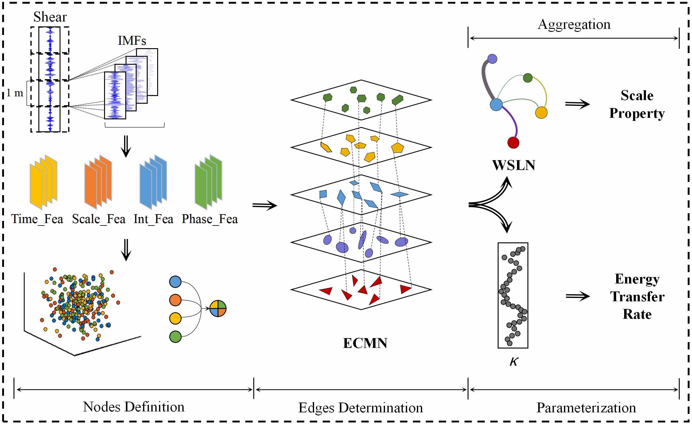
Figure 1 The skeleton of the proposed network model.

2.1 Definition of nodes

The translation of energy cascade characteristics into topology nodes is significant for the ECMN construction. Here, the energy evolution is evaluated and the physical feature statistics are extracted for node definition. And one node consists of four physical feature elements: time series, scale, local intermittency, and phase. The evaluation of energy features while cascading employs a range of algorithms, including the noise-assisted multivariate empirical mode decomposition (NA-MEMD), the wavelet analysis, the local intermittency measure (LIM), and the Hilbert transformation (HT). These algorithms are used to assess nonstationary features and chaotic motions [Vassilicos (2015); Alexakis and Biferale (2018)].

The NA-MEMD algorithm proves to be an efficient technique in decomposing unstable and nonlinear data, catering to various complex systems [Mohamed et al. (2022); Wang et al. (2022); Yuan et al. (2023)]. Compared to the empirical mode decomposition (EMD) [Huang et al. (1999), Huang et al. (1998)], the NA-MEMD helps to accurately tunes the corresponding intrinsic mode functions (IMFs) from multiple channels in the same frequency range [Rehman and Mandic (2011)]. Furthermore, the NA-MEMD has the advantage of the dyadic filter bank and the separability between the IMFs [Huang and Wu (2008)].

For a time series of turbulent signals x(t) measured by the MicroRider instrument, we divide each series into adjacent segments with a uniform depth of 1 meter (shown in Figure 1), and each individual segment is evaluated to construct the corresponding ECMN.

We employ the NA-MEMD method on these segments to obtain the corresponding IMFs, which enable the identification of underlying dynamic behaviors. Meanwhile, the time energy distribution of the corresponding IMF is analyzed using wavelet analysis [Gilles (2013)] by applying Equation 1:

$\begin{array}{ll}w{t}_{a,b}=\frac{1}{\sqrt{a}}{\displaystyle \underset{-\infty }{\overset{\infty }{\int }}{\text{Ψ}}^{*}}\left(\frac{t-b}{a}\right)IMFdt& (1)\end{array}$

where a is the scale dilation and b is the time parameter. The factor a^−1/2 guarantees the preservation of wavelet energy at all scales. Ψ represents the db10 mother wavelet function.

To identify the distribution of intermittent energy bursts at different IMFs, the LIM is applied to detect the local intermittency fluctuation [Onorato et al. (2000); Gopinath and Prince (2019)]. And it is given as Equation 2:

$\begin{array}{ll}LI{M}_{a,b}=\frac{{\left|w{t}_{a,b}\right|}^2}{{⟨{\left|w{t}_{a,b}\right|}^2⟩}_b}& (2)\end{array}$

where wt_a,b is the wavelet coefficient. The angled bracket represents the coefficient averaged over the time interval. This information is valuable for assessing the local energy level, particularly when the sample exceeds the average power level. Therefore, it aids in predicting energy accumulation and detecting intermittent bursts.

According to Yaglom’s law [Sorriso-Valvo et al. (2007)], energy transferred between different scales can either strengthen or weaken their amplitudes, which may result in phase synchronization in fluctuations.

As a result, the HT is performed on each IMF to determine the associated phase fluctuation

Using the aforementioned nonlinear algorithms, every turbulent segment x(t) is decomposed into a limited number n of IMFs with a narrow frequency spectrum. The corresponding scale parameter is determined by averaging over the entire time interval. Additionally, local intermittency time series and phase time series are obtained through equivalent IMF lengths. In order to preserve the fluctuation features, multivariate time series are split alone the sampling points. The corresponding variables of time t, scale s, local intermittency LIM and phase φ are integrated into the node quadruple V, e.g. $V_i=\left\{t_i,s_i,LI{M}_i,{\phi }_i\right\}$. Nodes of the same scale, i.e. derived from the same IMFs, are clustered together to form the single layer structure in the ECMN. Meanwhile, the layout of each layer resembles a coordinate axis space in which these cluttered nodes are arranged in chronological order.

2.2 Determination of edges

Edges in the network structure represent energy transfer between different scales. In the ECMN, node i and node j are adjacent at the point where energy is transferred between neighboring scales. Dynamical parameters in the node quadruple V are evaluated to determine whether a pair of nodes meet the qualifications and are connected to each other.

The local intermittency value is introduced to detect intermittent bursts indicating high local energy accumulation at a given time and specific scale. For each scale, the energy above the average is represented by the condition LIM> 1, within the time series. If LIM is less than 1, the energy has a lower distribution than the average. Therefore, the LIM peak is considered to be an effective indicator to identify the energy bursts, which represent massive energy accumulation during turbulence evolution.

Based on solar wind magnetic turbulence, Perri [Perri et al. (2012)] confirmed the coexistence of phase synchronization and energy transfer processes between pairs of neighboring scales. The phase of two mode is found overlapped, and their phase difference becomes negligible when energy is transferred between two eddies with different scales. Thus, the phase synchronization between each pair of modes (IMF_i, IMF_j) is applied to determine the location of turbulent energy bursts and the occurrence of energy transfer between different scales.

Therefore, the rules that we followed to determine edges are as follows:

(1)two synchronous nodes on different scales are selected for evaluation;

(2)their LIM value should be above the average;

(3)the simultaneous LIM peaks should be observed;

(4)the phase difference is close to zero;

A pair of nodes can be found connected by an edge if the above rules are satisfied. On the contrary, node i and node j are isolated if one of these conditions is not fulfilled.

2.3 Aggregation

The ECMN framework is represented by M = ⟨V, E, L⟩. Each node i in M is a multivariate quadruple and is a member of the node set V. Meanwhile, E represents the edge set and denotes the layer set. The network tuple (i, α) is defined to describe the bond relationship in which node i exists on the layer α.

The structure of ECMN differs from that of other multi-layer networks. In this study, we focus on the process of energy transfer between pairs of neighboring scales. Thus, in the ECMN, active nodes are only connected by the inter-layer edges, denoted as $E_{\alpha \beta }=\left\{((i,\alpha ),(j,\beta ))\in E\mid \alpha \ne \beta \right\}$. Active node i, which belongs to layer α, and active node j, which belongs to layer β, are adjacent from two neighboring layers. However, nodes, mentioned in other multi-layer structures, are also connected by intra-layer edges in the same layer [Boccaletti et al. (2014)], given as $E_{\alpha \beta }=\left\{((i,\alpha ),(j,\beta ))\in E\mid \alpha =\beta \right\}$.

Here, a WSLN structure is applied to aggregate effective elements, remove pinheads and ultimately concentrate the topological multi-layered network into a new single-layer structure. It helps to extract energy transfer contributors. Active nodes and inter-layer edges are identified as useful elements to reconstruct this single-layer network, while isolated nodes are removed as unnecessary. Furthermore, active nodes in the Layer α of ECMN are integrated to form a new layer-node in the single-layer network, named ‘Layerα’. According to the operation, scale and the layer energy (LE) are integrated in the new node tuple, namely $Layer\alpha =\left\{s_{\alpha },L{E}_{\alpha }\right\}$. The LE is captured by the marginal Hilbert spectrum h(f) as it represents the energy contribution to the original signal. And it can be calculated as follows:

$\begin{array}{ll}h(f)={\displaystyle \underset{0}{\overset{T}{\int }}H}(f,t)dt& (3)\end{array}$

where $H(f,t)$ is the Hilbert spectrum in Equation 3.

In addition, the inter-layer edges in the ECMN are merged as new edges d_αβ in the WSLN. d_αβ is assumed to be active if any pair of nodes in layer α and layer β are adjacent. The weight W_αβ of d_αβ is defined as the number of corresponding inter-layer edges.

2.4 Network structure coefficient

The proposed multi-layer model uses inter-layer edges to denote the process of energy cascade. The parameterization of these inter-layer edges can provide the underlying information about the strength of energy mixing. In cascade theory, it is assumed that the energy input at the large scale is equal to the energy dissipated in the small scale. In other words, the energy flux is constant, on average. The large-to-small coupling is demonstrated to exist locally in scale, space and time (Meneveau and Lund (1994)). Meanwhile, the causal connection between energy cascade and dissipation has been amply demonstrated (Cardesa et al. (2015); Cardesa et al. (2017); Ballouz et al. (2020); Vela-Martin (2022)). Therefore, the network structure coefficient is introduced here to quantify the amount and weight of inter-layer edges and investigate the validity of the proposed model. Based on network attributes, the network structure coefficient κ is obtained by Equation 4:

$\begin{array}{ll}\kappa ={\displaystyle \sum _{\alpha \beta \subset L}\frac{N}{{\eta }_{\alpha \beta }(s_{\alpha }+s_{\beta })}}& (4)\end{array}$

where η_αβ represents the quantity of inter-layer edges linking layer α with layer β, N is the total number of nodes in layer α, and s_α +s_β denotes the scale weight influenced by the typical features of the neighboring layers.

3 Observations and data processing

Because of their crucial role in the ocean circulation, data measured from the SYS [Pang et al. (2017); Teng et al. (2017); Yuhua et al. (2017)] and the SCS [Chunhua et al. (2019); Tan et al. (2021)], which are characterized by energetic currents (Figure 2A), were analyzed. The measurements were taken on 22-24 September 2021 at St. A (35°32'N,121°14'E, the mean water depth around 38 m) and on 12 December 2020 at St. B (19°39'N,115°27'E, with the mean water depth close to 1500 m). Due to the limitation of cable length, only the fluid statistics over 300 m were observed at St. B.

Figure 2

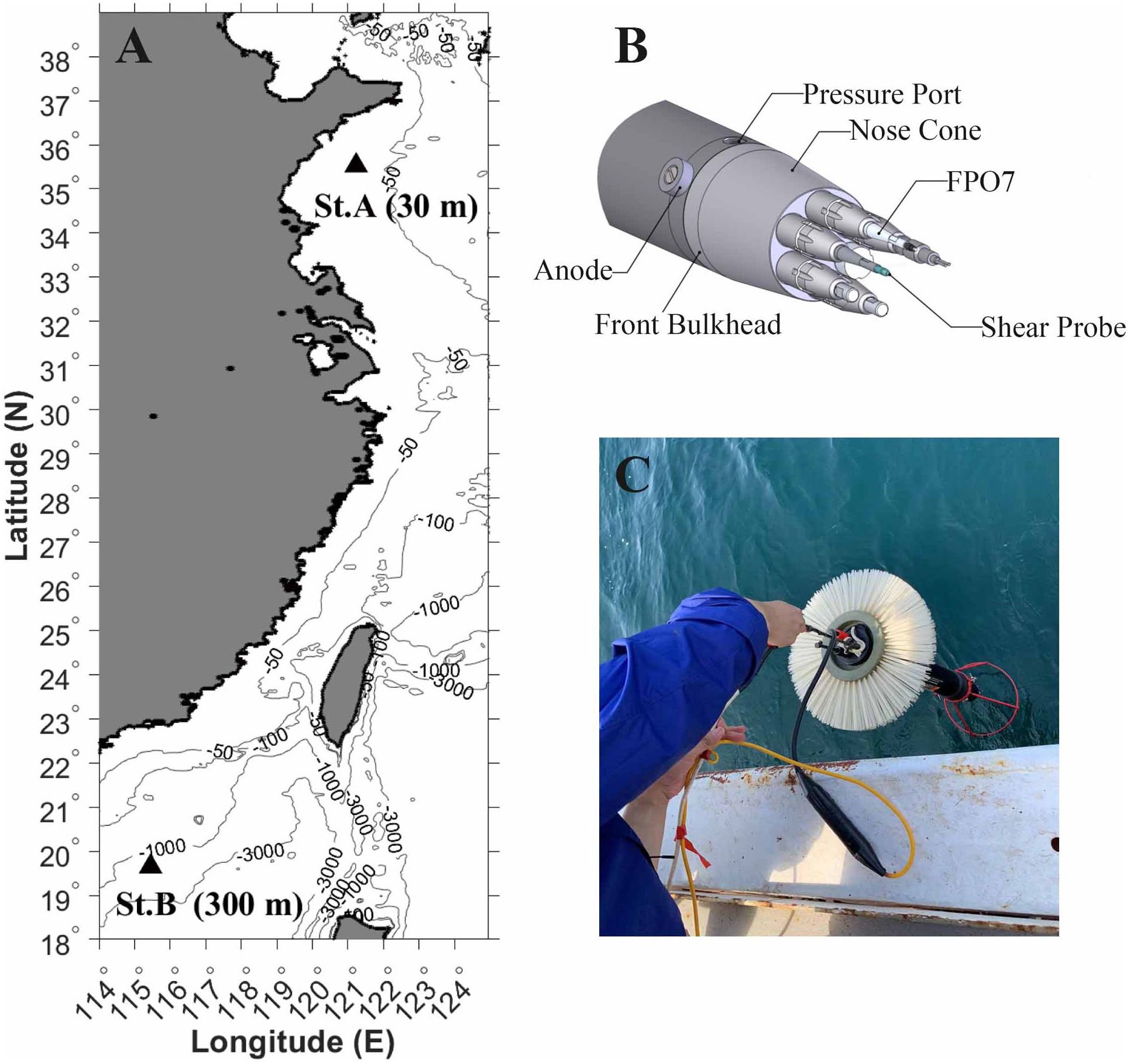
Figure 2 (A) Bathymetric map. The locations of measurement station are denoted by black triangle. (B) MicroRider sensors. (C) MicroRider just before deployment in the ocean.

Vertical microstructure and mixing signatures were examined using hydrographic data. The vertical microstructure was investigated using the MicroRider instrument (Figure 2B), manufactured by the Rockland Scientific International (RSI). The MicroRider nose cone contains a pair of orthogonal velocity shear probes, a high-resolution temperature probe, an accelerometer and a pressure sensor, with sampling rates all at 512 Hz. During the observations, the MicroRider instrument was released from the stern deck, which was loosely tethered with a tether (Figure 2C).

The dissipation rate of turbulent kinetic energy ε [Wolk et al. (2002), Gregg (1999), Roget et al. (2006)], which quantifies the intensity of the turbulent mixing, can be obtained under the assumption of isotropic turbulence by integrating the power spectra over the wavenumber k.

$\begin{array}{ll}\epsilon =\frac{15}{2}\nu {\overline{\left(\frac{\partial u}{\partial z}\right)}}^2=\frac{15}{2}\nu {\displaystyle {\int }_{k_{\text{min }}}^{k_{\text{max }}}\text{Φ}(k)dk}& (5)\end{array}$

where ν is the kinematic molecular viscosity (nearly $1\times {10}^{-6}{m}^2{s}^{-1}$ $\overline{{(\partial u/\partial z)}^2}$ is the variance of vertical shear, and Φ(k) is the power spectrum of shear in Equation 5. The power spectrum is integrated within the inertial domain $(k_{min}<k<k_{max})$. Here, k_min and k_max are the lower and upper wavenumber limits for integration, respectively. In the operation, the k_min is assumed to be 1 cpm (cycles per meter). The low wavenumber range $(k<k_{min})$ cannot be detected by the MicroRider. The apparent high wavenumber peaks $(k>k_{max})$ are caused by instrument vibration which interferes with the shear signals.

Figure 3 shows the vertical variation. There are peaks in the pitch variation corresponding to different types of disturbance. Above a depth of 5m, wave action caused instrument disturbance and slight pitching of the MicroRider (Figure 3A). The instrument entered a stable dive mode with an average rate of descent of 0.6 m/s (Figure 3B). A sharp drop in temperature indicates a strong pycnocline at 25m at St A and 105m at St B (Figure 3C). The pycnocline separates the water column into well-mixed surface, thermocline and bottom boundary layers in the horizontal direction. The stratification inhibits the turbulent mixing and vertical redistribution of marine material [Sharples and Simpson (2012)], as indicated by the sharp decrease in dissipation rate in Figure 3F. Below the pycnocline, a seasonal cold water mass occupies the water column and dominates the hydrological flow evolution [Fangli et al. (2011); Kyung-Hee et al. (2012); Fan (2016), Brown et al. (1999)], which is growing in spring, maturing in summer, decreasing in autumn and winter. Meanwhile, strong stratification causes relative tilting and disturbances in the vicinity of junctions. Therefore, the Goodman coherent noise reduction algorithm is applied to reduce the contamination in the shear measurements and to calibrate for the instrument vibration (Goodman et al. (2006)). The perturbation variation of shear is first extracted by comparing the original shear and its mean variation. The contamination was then removed by subtracting all of the coherent fluctuations between the shear perturbation variation (Figure 3E) and the accelerometer variables (Figure 3D). Figure 3G shows the shear power spectrum at stable depth, the blue and orange curves represent the shear power spectrum, the black line indicates the Nasmyth spectrum and the solid triangle represents the cutoff wavenumber. Within the cutoff wavenumber limit, the shear curves are found to almost overlap with the Nasmyth curves (Figure 3G), and this means that the shear spectrum is well matched to the standard Nasmyth spectrum, indicating effective data for the following turbulence analysis. Figure 3F illustrates the vertical turbulent mixing. Under the combination of wind and terrain frictions, the turbulent mixing intensifies in the surface and boundary layers of the SYS water column with a dissipation rate magnitude close to 10⁻⁷. Meanwhile, turbulent mixing is inhibited in the well-mixed thermocline layer with an average dissipation magnitude of 10⁻⁹. The vertical variation of the dissipation rate in the SYS is consistent with the description in previous researches [Xu et al. (2020); Song et al. (2021)]. Owing to the wind stress and buoyancy flux, the depth of mixing layer depth in the SCS is much deeper in winter. Due to the limited cable length, only the microstructure data in the surface and stratification layers were measured. The thermocline also impedes turbulent mixing in the water column in the SCS. Meanwhile, the wind stress stimulates turbulent mixing in the surface and its corresponding mixing magnitude is nearly 10⁻⁷, which is two orders higher than that in the thermocline (10⁻⁹) [Iossif (2012); Wang et al. (2012); Xiao et al. (2013)].

Figure 3

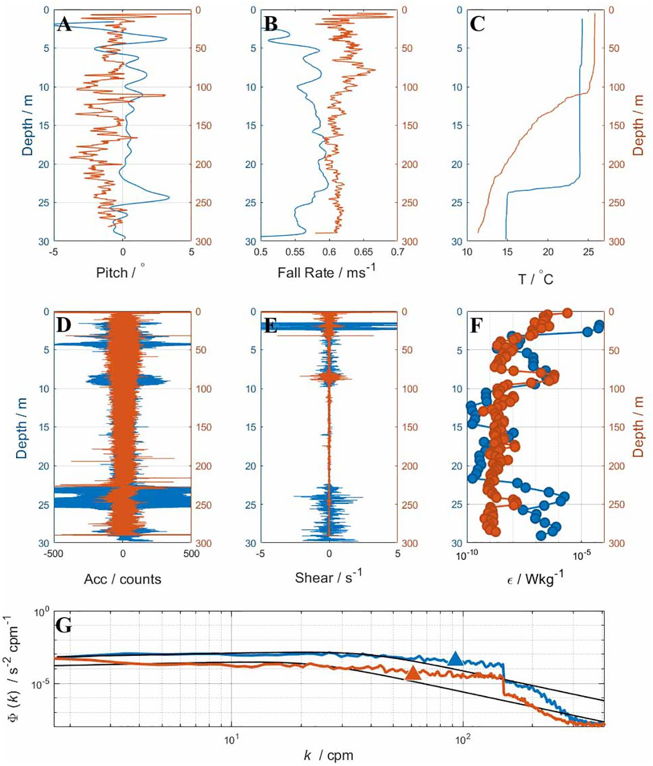
Figure 3 Vertical variations of the microstructure collected at St. A and St. B, represented by blue and orange curves, respectively. (A) The pitch angle of the instrument axis. (B) The fall rate of the instrument. (C) The vertical temperature profile. (D) The vertical acceleration profile. (E) The vertical shear profile. (F) The associated dissipation rates. (G) The associated shear spectrum (blue and orange curves) and the corresponding Nasmyth spectrum (black line).

4 Results

The entire shear signal is divided into uniform segments with 1 m to characterize the turbulent evolution in each vertical profile. Considering the diving stage of the instrument, depth segments of 6 m, 16 m and 26 m derived from the profile collected at St. A are selected to show their corresponding multi-layer frameworks. For the same reason, network structures are inferred from depth segments of 30 m, 80 m, 130 m, 180 m, 230 m and 280 m of the profile measured at St. B. These depth segments represent, in order, the initial phase, the sustained phase of stable diving, the turbulent phase crossing the thermocline and the near-bottom phase, respectively.

The energy cascade process is mapped by the network structure and topological features of the ECMN. Nodes and edges in the ECMN are depicted in a three-dimensional space with the following axes: x, which represents the time series; y, which indicates the intrinsic scale properties, network layers are arranged along the y axis, and the time scale decreases along the y−direction; and z, which indicates the local intermittency, indicating the energy accumulation of each node. Furthermore, a pair of simultaneous nodes (i, α) in layer α and (j, β) in layer β are adjacent to each other by an inter-layer edge e_αβ if they satisfy the qualification of edge determination. The inter-layer edge e_αβ represents the occurrence of energy transport between scales S_α and S_β.

Figures 4A–C show the corresponding ECMN built from shear segments at 6 m, 16 m, and 26 m, respectively. Shear signal in each segment is decomposed into several IMFs, and physical feature statistics are extracted at each sampling point of the IMF. Each node is a data collection containing time variable, scale variable, local intermittency variable and phase variable. Scattered nodes are assigned to a particular layer according to the scale feature, i.e. nodes derived from the same IMF are located at the identical layer. Here, layers are represented by transparent gray planes and nodes located on the identical layer are colored the same. Nodes with the shortest scale are located in the front right plane and are colored blue (Figure 4). Other nodes are located in the back layers and to the left as scale increases. Nodes with the largest scale feature are colored red in Figures 4A, C. Meanwhile, nodes with the largest scale are colored gray in Figure 4B. Furthermore, the location of nodes in a particular layer varies according to the time (x−direction) and energy properties (z−direction). In addition, the black dashed lines represent the connection between pairs of simultaneous nodes in different layers and they indicate the occurrence of energy transfer across scales.

Figure 4

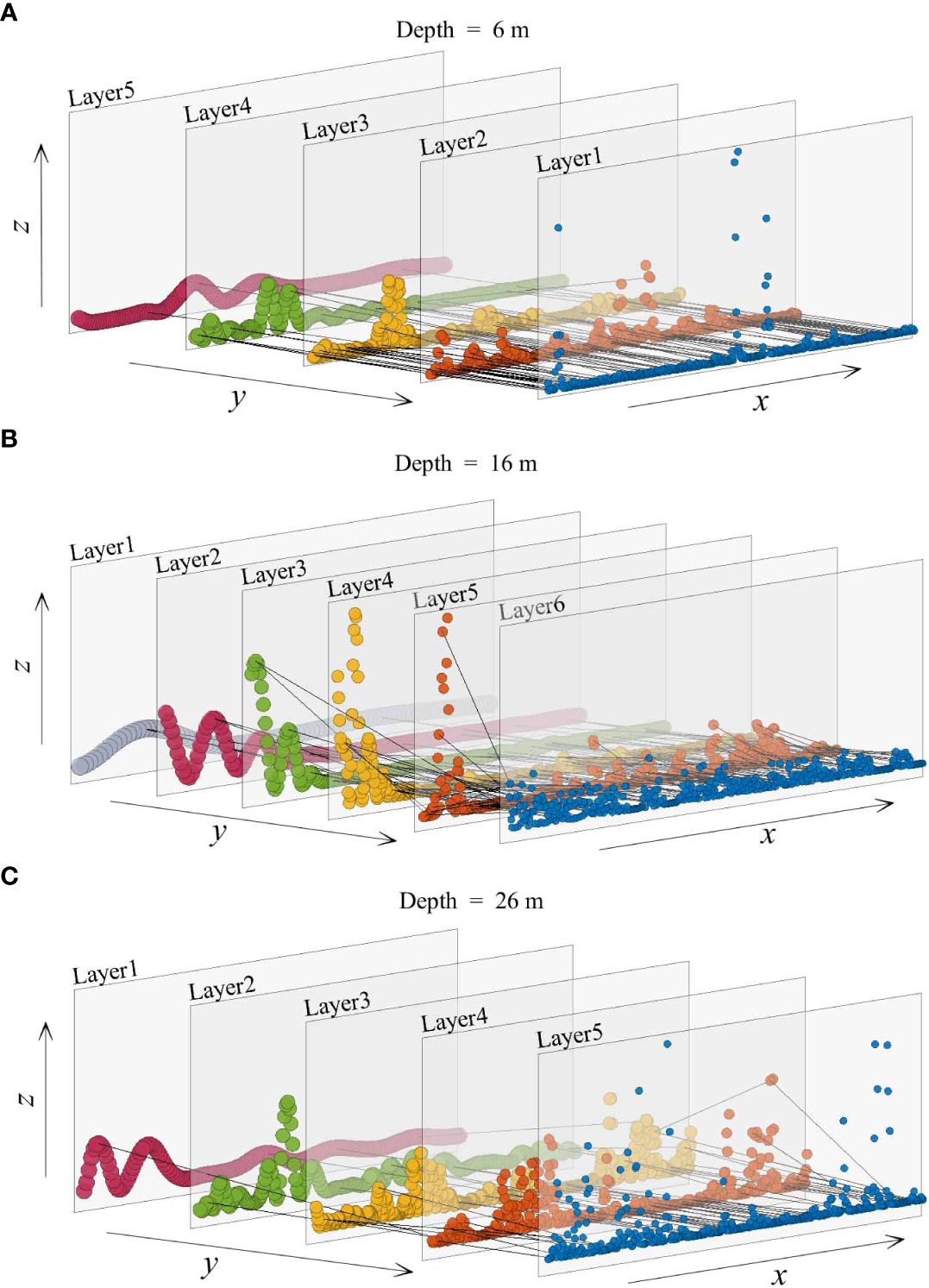
Figure 4 The ECMN constructed from the shear variation at the 6m, 16m and 26m depth segments and their corresponding subplots. Nodes with specific scales are indicated by different colors. Active layers and their energy-receiving layers are connected by inter-layer edges (dashed lines). (A) The ECMN constructed from the shear variation at the 6 m depth segment. (B) The ECMN constructed from the shear variation at the 16 m depth segment. (C). The ECMN constructed from the shear variation at the 26 m depth segment.

Figures 5A–F show the corresponding ECMN constructed based on shear segments at 30 m, 80 m, 130 m, 180 m, 230 m and 280 m, respectively. Taking the Figure 5A as an example, the underlying energy cascade process in the 30 m depth segment is converted into a topological framework. The shear signal s(t) in the 30 m depth segment is decomposed into six IMFs. Wavelet analysis, LIM and HT algorithms are performed on IMF1-IMF6 to evaluate the underlying characteristics. For each IMF, we will obtain three variations of time, local intermittency and phase, and a fixed value of scale. Physical statistics obtained at the same sampling point and the scale value together form topological nodes. A total of 412 nodes are obtained in this segment, and they are spread out in different locations according to their feature variables. Meanwhile, the feature variables in each pair of nodes i and j from different layers are evaluated to estimate whether they satisfy the requirements and determine the existence of edge.

Figure 5

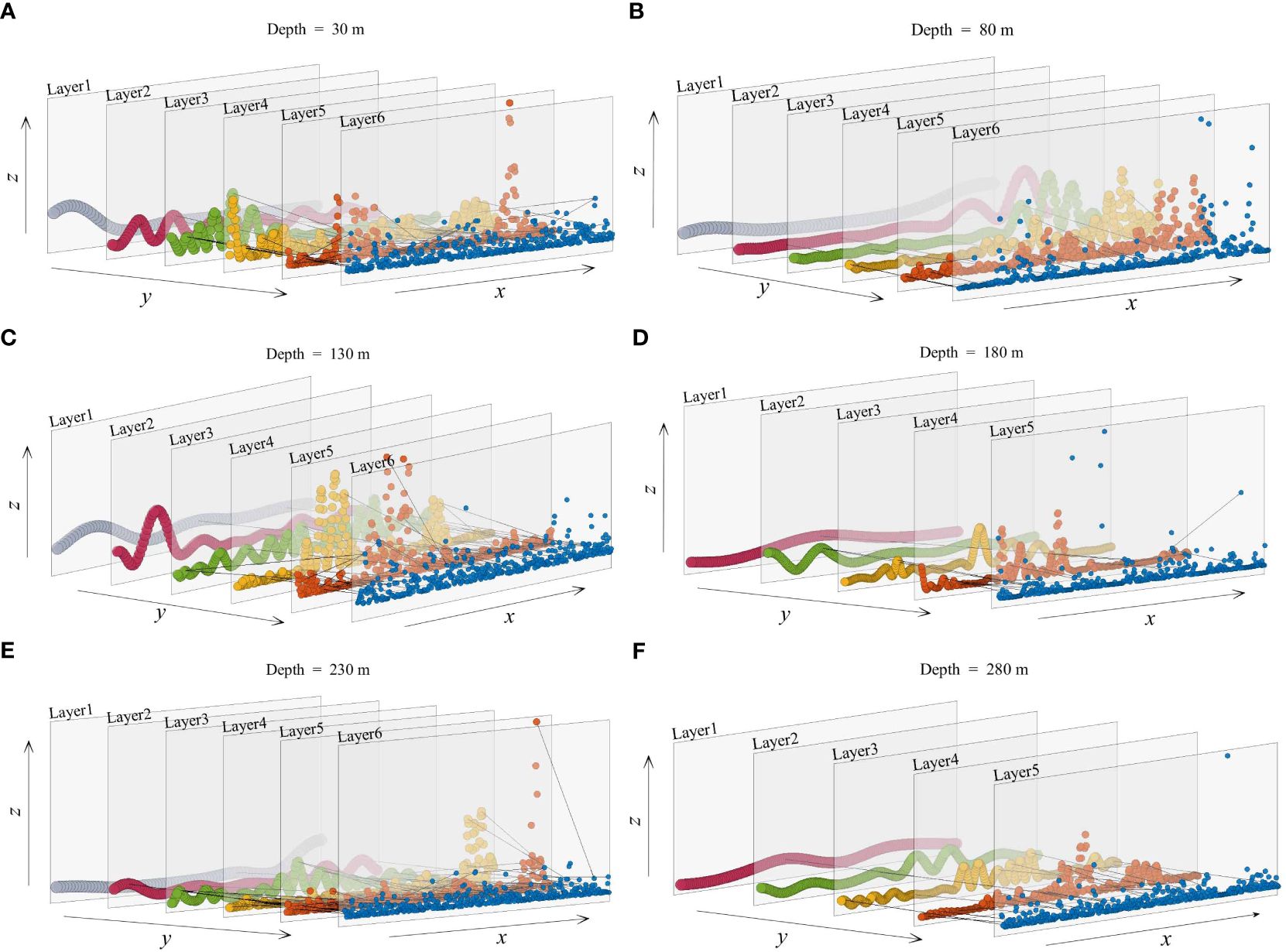
Figure 5 The ECMN constructed from shear variations at the depths of 30m, 80m, 130m, 180m, 230m and 280m. Nodes with specific scales are indicated by different colors. Active layers and their energy-receiving layers are connected by inter-layer edges (dashed lines). (A) The ECMN constructed from the shear variation at the 30m depth segment. (B) The ECMN constructed from the shear variation at the 80m depth segment. (C) The ECMN constructed from the shear variation at the 130m depth. (D) The ECMN constructed from the shear variation at the 180m depth. (E) The ECMN constructed from the shear variation at the 230m depth. (F) The ECMN constructed from the shear variation at the 280m depth segment.

We assume that different layers have different physical meanings, which are associated with different powers and frequencies. The marginal Hilbert spectra (Figure 6) for each depth segment indicate the contribution and distribution of the turbulent energy across frequencies. According to the marginal Hilbert spectra, larger scale layers generally have higher peaks (such as the red curves in Figures 6A, C, G, I, and the grey curves in Figures 6B, D-F, H), representing the mean flow with overwhelmingly large energy and sustaining the primary ocean circulation. In addition, smaller scale layers are usually found with relatively low energy. Herein, we ideally assume that all of the turbulence energy is transferred from the large scale to the small scale. Thus, the larger scale layer is the energy-producing layer and the smaller scale layer corresponds to the energy-receiving scale.

Figure 6

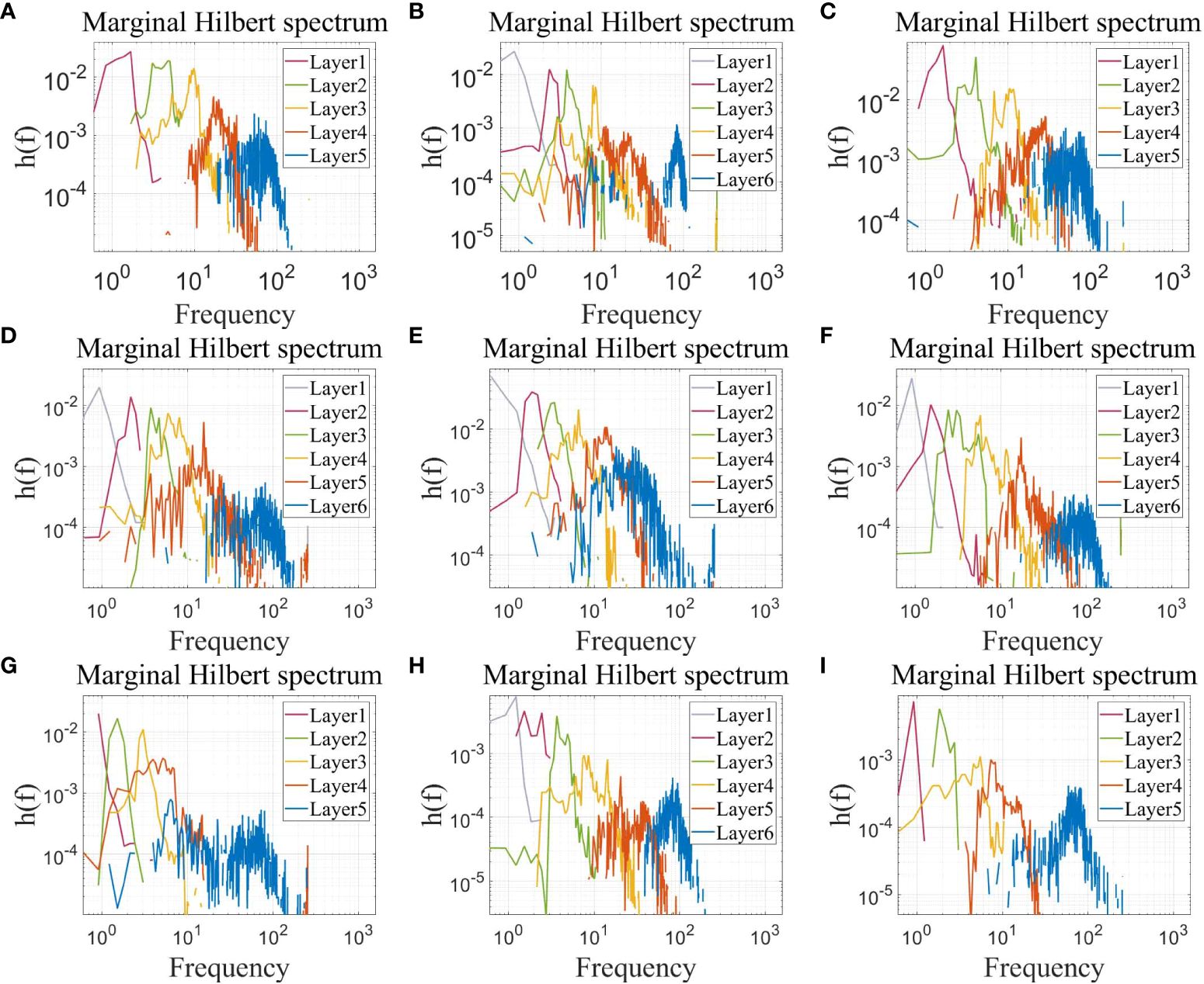
Figure 6 The marginal Hilbert spectra for St. A depth segments at (A) 6 m, (B) 16 m, and (C) 26 m. The marginal Hilbert spectra for St. B depth segments at (D) 30 m, (E) 80 m, (F) 130 m, (G) 180 m, (H) 230 m, and (I) 280 m.

The details of the ECMN are shown more clearly in Figures 7–10 (others in the Supplementary Material), where the overlapping edges between layers and their connected layers in Figures 4, 5 are separated into these sparse subgraphs, respectively. The sparse distribution of inter-layer edges indicates the inhomogeneity of energy cascade evolution. The energy transfer interaction between Layer 2 and its energy-receiving layers is relatively intense at the 6 m segment (Figure 7B). On the other hand, few inter-layer edges are found at the 26 m segment (Figure 9B). Meanwhile, the energy in Layer 1 (Figure 10A) is very stable and less energy is detected to be transferred from Layer 1. However, Layer 1 in Figure 5B is isolated from other layers, which maintain relatively quiescent energy, and no energy is transferred to small scales. In addition, the inter-layer edge distribution indicates the inhomogeneity in scale interaction. The inter-layer edges adjacent to Layer 3 and the its energy-receiving layers are shown in Figure 8C. It describes an energy transfer process, in which a small amount of energy in Layer 3 cascades to Layer 4, Layer 5 and Layer 6. In contrast, the scales derived from Layer 3 differ from those derived from Layer 2 (Figure 8B) or Layer 4 (Figure 8D). Energy in Layer 2 (Figure 8B) in found to be transferred to Layer 3-6 and turbulence energy in Layer 4 (Figure 8D) is found to be transferred to Layer 5-6. The inter-edges intensity increases as the energy of the scales decreases. Meanwhile, dramatically dense existences of inter-layer edges are found at the ends of subgraphs, indicating strong energy transfer between these miniature scales. The distribution of inter-layer edges and specific energy-receiving scales in each ECMN indicates that the characteristics of evolution and scale are dramatically intermittent and inhomogeneous.

Figure 7

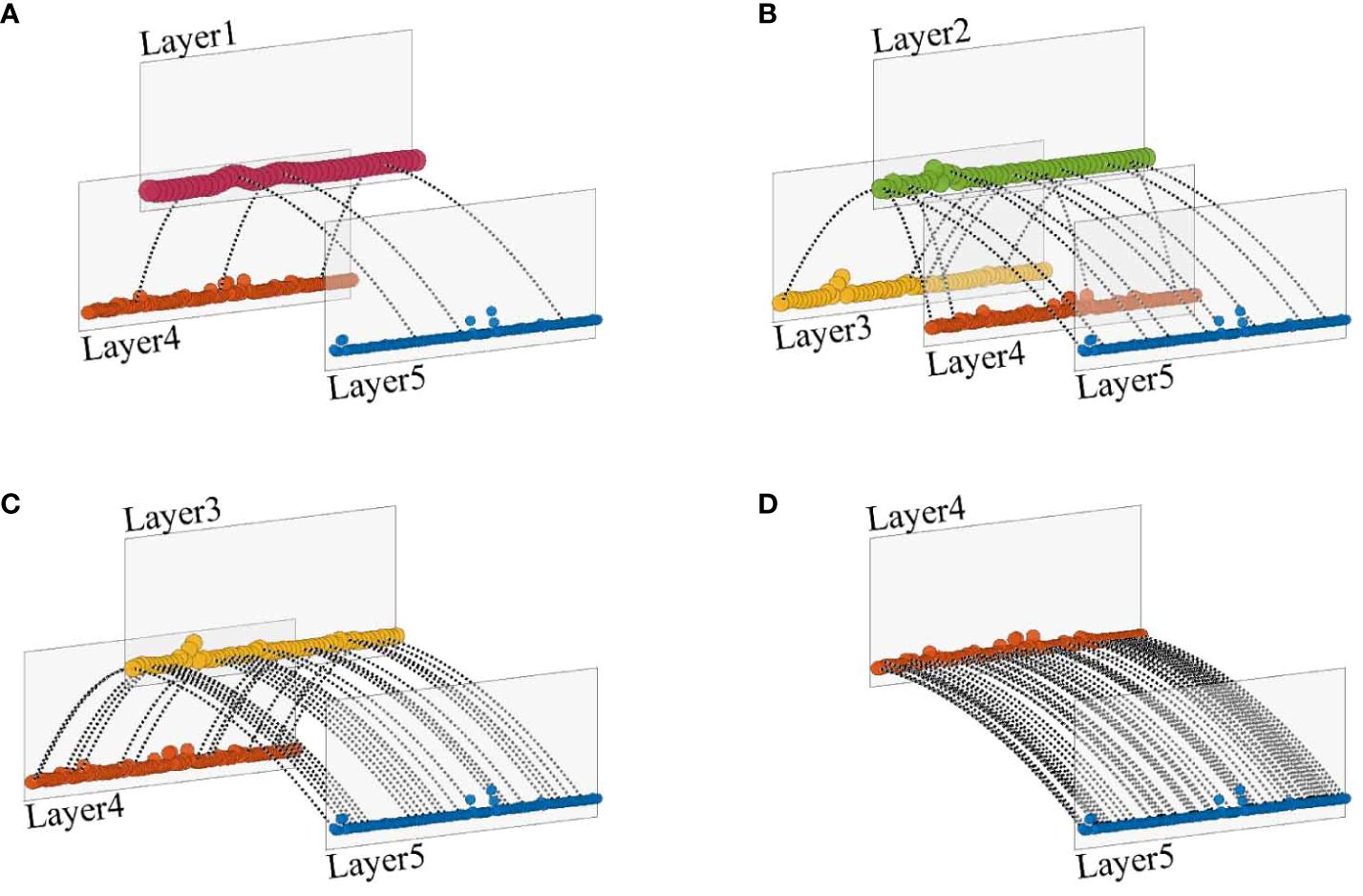
Figure 7 Sparse subgraphs of Figure 4A. (A) The energy in Layer 1 is found to be transferred to its energy-receiving layers, including Layer 4 and Layer 5. (B) All inter-layer edges that are connected to Layer 2 and its energy-receiving layers. (C) Layer 3 and its corresponding energy-receiving layers are presented. (D) Energy in Layer 4 is only transferred to Layer 5.

Figure 8

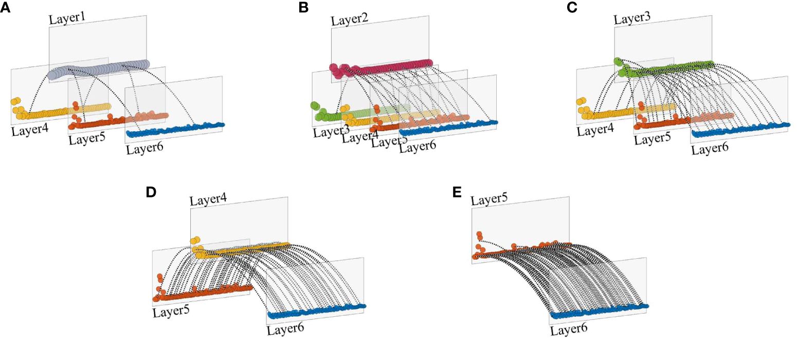
Figure 8 Sparse subgraphs of Figure 4B. (A) The energy in Layer 1 is found to be transferred to its energy-receiving layers, including Layer 4, Layer 5 and Layer 6. (B) All inter-layer edges that are connected to Layer 2 and its energy-receiving layers. (C) Layer 3 and its corresponding energy-receiving layers are presented. (D) The energy in Layer 4 is transferred to Layer5 and Layer 6. (E) The energy in Layer 5 is only transferred to Layer 6.

Figure 9

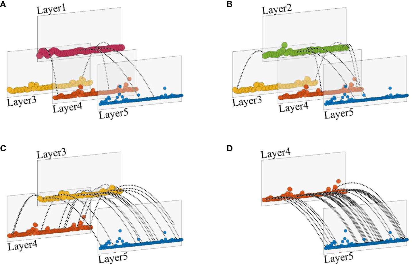
Figure 9 Sparse subgraphs of Figure 4C. The energy in both (A) Layer 1 and (B) Layer 2 is transferred to Layer 4, Layer 5 and Layer 6. (C) Layer 3 and its corresponding energy-receiving layers, Layer 4 and Layer 5. (D) The energy in Layer 4 is only transferred to Layer 5.

Figure 10

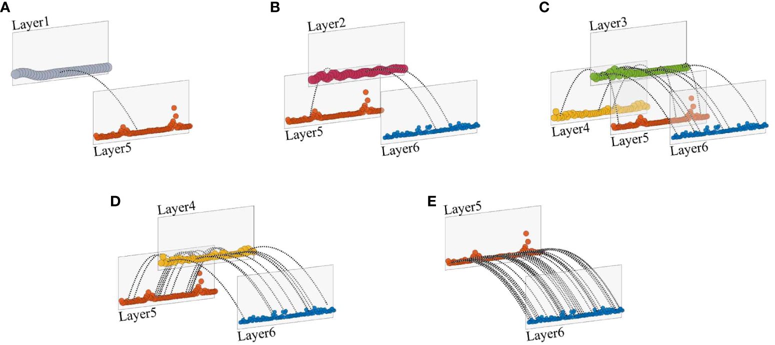
Figure 10 Sparse subgraphs of Figure 5A. (A) The energy in Layer 1 is only transferred to Layer 5. (B) All inter-layer edges that are connected to Layer 2 and its energy-receiving layers. (C) Layer 3 and its corresponding energy-receiving layers, Layer 4, Layer 5 and Layer 6. (D) The energy in Layer 4 is transferred to Layer5, and Layer 6. (E) The energy in Layer 5 is only transferred to Layer 6.

Subsequently, the aggregation method is applied to investigate the scale property of the energy cascade under the multi-layer framework. Each depth segment is divided into two equal sections. The first half and the second half of the ECMN are aggregated into corresponding WSLN, respectively (Figures 11, 12). Here, the node sizes vary with the corresponding energy and the line width represents the weight of edge in the aggregated WSLN. Fine edges can be seen extending from the larger nodes (Figure 12A1). In particular, Layer1 is separated from the others in Figure 12A2. This implies that these energetic structures have settled into a relatively stationary state, with little energy observed from them. Meanwhile, nodes of intermediate energy are identified as relatively active and some of the energy contained within them is transferred to finer structures via inter-layer edges (Figure 12E1). The largest weight, indicating enormous inter-layer edges, appears in the pair of smallest nodes, e.g., Layer5 and Layer6 in Figure 11B1. And it is much more visible in Figure 11B2. Moreover, almost all of the nodes are connected to these small or miniature structures. In each step, the staple concentration of energy in the ‘active eddies’ tends to cascade directly to small or miniature structures [Josserand et al. (2017)] compared to other generated structures (e₁₆ in Figure 11B1, e₁₆ in Figure 12C2, e₁₅ in Figure 12E2). The same results can be obtained from the degree normalization histogram (Figure 13). Small layer-nodes have dramatic peaks of overwhelming magnitude. Therefore, these nodes are characterized as radical fighters that contribute significantly to the energy transfer. In other words, larger scale energy structures are stable participants, controlling the relatively monolithic stability of the turbulence system. Nevertheless, these small eddies disturb this stable system and promote the evolution of turbulent mixing.

Figure 11

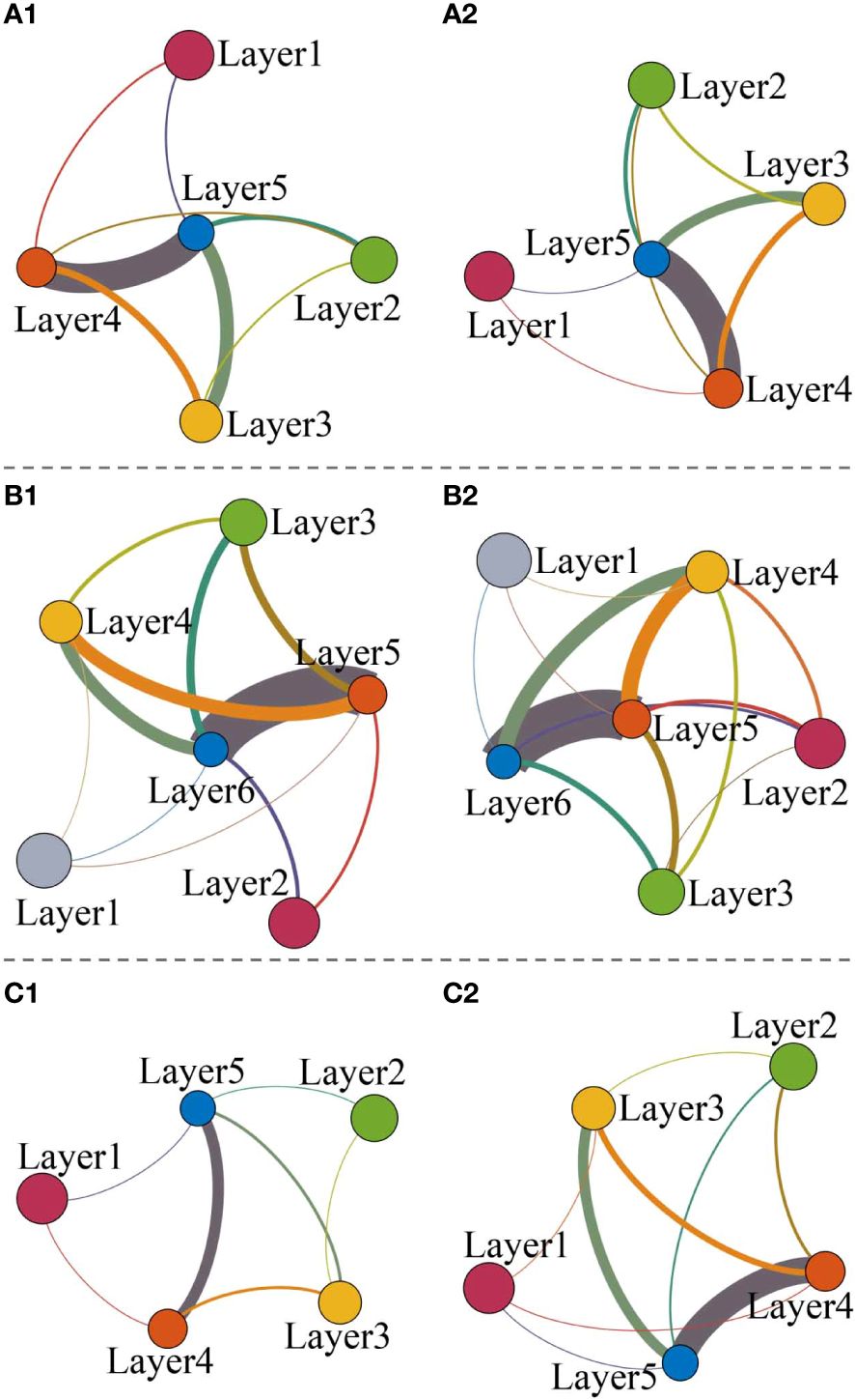
Figure 11 The WSLN aggregated from (A1) the first half and (A2) the second half of the corresponding ECMN in Figure 4A. The WSLN aggregated from (B1) the first half and (B2) the second half of the corresponding ECMN in Figure 4B. The WSLN aggregated from (C1) the first half and (C2) the second half of the corresponding ECMN in Figure 4C.

Figure 12

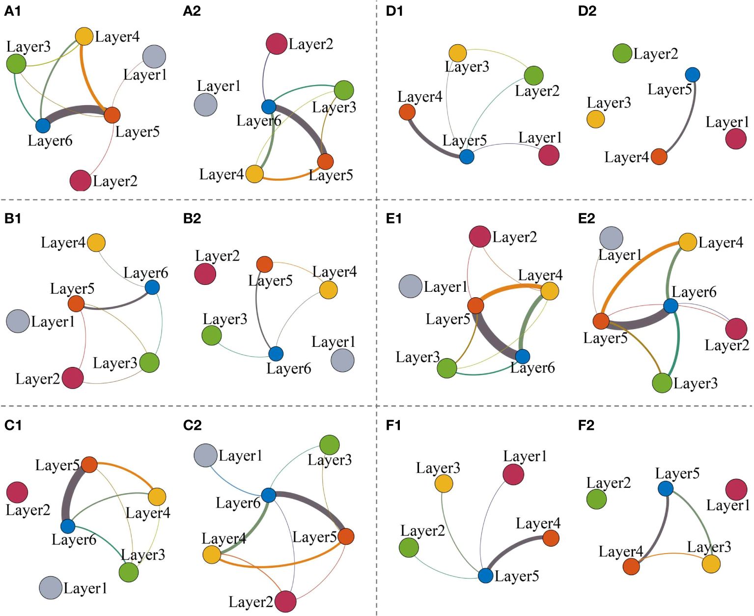
Figure 12 The WSLN aggregated from (A1) the first half and (A2) the second half of the corresponding ECMN in Figure 5A. The WSLN aggregated from (B1) the first half and (B2) the second half of the corresponding ECMN in Figure 5B. The WSLN aggregated from (C1) the first half and (C2) the second half of the corresponding ECMN in Figure 5C. The WSLN aggregated from (D1) the first half and (D2) the second half of the corresponding ECMN in Figure 5D. The WSLN aggregated from (E1) the first half and (E2) the second half of the corresponding ECMN in Figure 5E. The WSLN aggregated from (F1) the first half and (F2) the second half of the corresponding ECMN in Figure 5F.

Figure 13

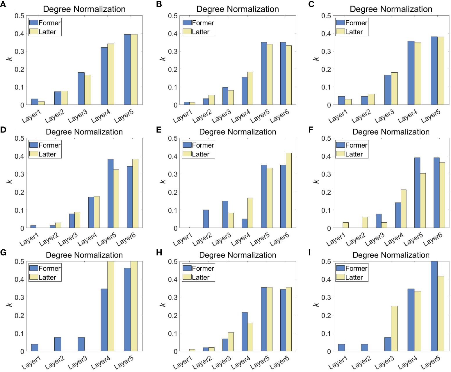
Figure 13 Degree normalization for St. A depth segments at (A) 6 m, (B) 16 m, (C) 26 m. Degree normalization for St. B depth segments at (D) 30 m, (E) 80 m, (F) 130 m, (G) 180 m, (H) 230 m and (I) 280 m.

Cascade is traditionally defined as a process in which energy is continuously transferred from one scale to the next in a decreasing order of magnitude Cardesa et al. (2015). However, the WSLN framework and its offshoots suggest that the mechanism of energy cascade differs significantly from that of homogeneous cascade models. And it suggests a synchronous multi-scale energy cascade pattern in which energy in one scale is synchronously transferred to all or part or none of the structures with smaller scales. Energy in node Layer2 (Figures 11A1, A2) is transferred to all layers of smaller scale. Energy in node Layer3 (Figures 11B1, B2) is transferred to all of the nodes with smaller scale. However, node Layer2 is only connected to node Layer5 in the first half of the 30 m depth segment (Figure 12A1) and node Layer2 is connected to node Layer3 and node Layer5 in the first half of the 80 m depth segment (Figure 12B1), indicating a large scale gap in energy transfer. Node Layer2 is connected to all smaller scales (Layer4, Layer5, Layer6) in Figure 12C2. However, the node Layer2 becomes isolated, and impedes energy transfer in the previous one (Figure 12C1). Similarly, Layer2 is adjacent to Layer4 and Layer5 in Figure 12E1, but it is connected to Layer5 and Layer6 in Figure 12E2, indicating a scale interruption. Furthermore, despite the similarity of the connections of the node pairs, the weight of the corresponding edges is completely different, implying the different intensity of energy transfer (Figures 11, 12), indicating the strong intermittency and inhomogeneity in the evolution of the energy cascade.

In addition, the network framework, based on marginal Hilbert spectra, covers both the inertial and dispersive regions of the turbulent power spectrum, allowing full identification of structures at all scales generated by the energy cascade. Meanwhile, syncretic signals are separated into isolated elements with relatively narrow frequency ranges and it characterizes full details of energy transfer between these structures of varying scales, providing a novel approach to turbulence analysis in the future.

The network structure coefficient κ is estimated to parameterize the energy transfer strength based on the specific layer scale and the number of inter-layer edges. The performance of is estimated with the microstructure profile. The variations of κ (shown in Figure 14) are in good agreement with the vertical profile of the dissipation rates. The shading represents the standard deviation of the dissipation rates. The correlation coefficients between κ and ϵ are 0.82 and 0.91 respectively, indicating a strong positive relationship. Thus, the ECMN framework is shown to be a valid structure for uncovering the underlying mechanism of the energy cascade, and κ is verified as an effective parameter for quantifying energy transfer. Furthermore, due to the strong stratification the κ estimates exhibit an abrupt increase around the pycnocline and are qualified to detect turbulent mixing oscillations. Thus, it shows generally good agreement in both strong mixing and well mixed regions, and the ECMN can be verified as an effective model for characterizing the underlying evolution of turbulent mixing.

Figure 14

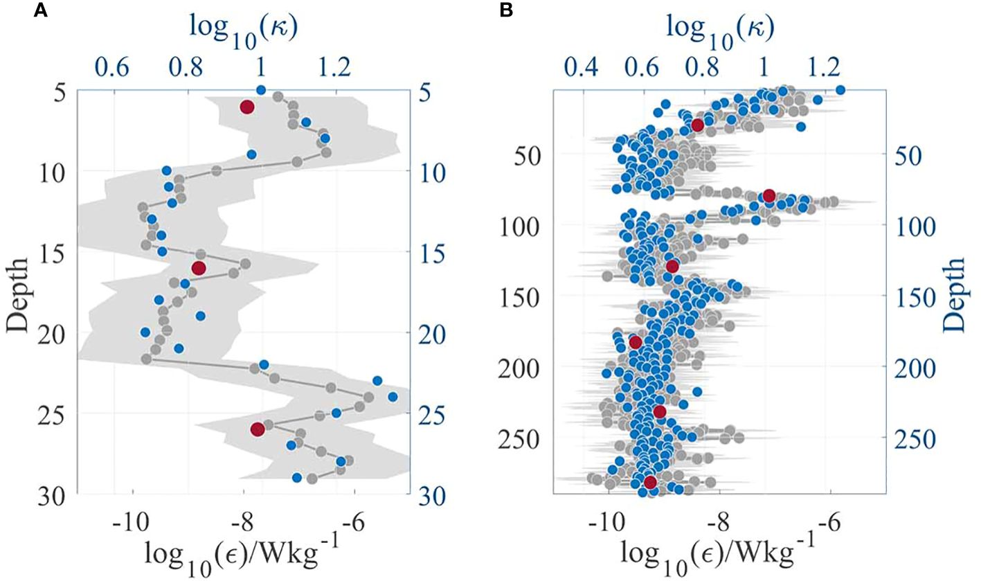
Figure 14 The performance of network structure coefficient κ. Vertical variations of dissipation rates ϵ and the network structure coefficient κ. The dissipation rates are represented by gray nodes, the standard deviation is shaded, and the network parameters are represented by blue nodes. (A) κ estimated at depths of 6 m, 16 m and 26 m are overlapped by red nodes. (B) κ calculated at depths of 30 m, 80 m, 130 m, 180 m, 230 m and 280 m are marked by red nodes.

5 Conclusions

Larger eddy decomposition and smaller vortex generation promote ocean circulation and turbulent mixing. The study of energy cascade is significant in oceanic studies. In the present work, the complex network analysis is used for the study of the chaotic interaction and scale property in energy cascade. An energy cascade multi-layer network (ECMN) was constructed, where nodes represent physical multivariate of turbulent fluid and inter-layer edges are indicators of energy transfer between scales. In the network, the underlying interactions of the energy cascade are transformed into topological elements, and the dynamic evolution of turbulent mixing can be revealed based on the topological property. In addition, the network framework covers both the inertial and dispersive regions of the turbulent power spectrum, allowing full identification of structures at all scales generated by the energy cascade. For a more detailed consideration of highly connected nodes, effective components in a multi-layer structure are aggregated into a single-layer network for both network analyses.

According to the topological framework of ECMN, the energy cascade process contradicts the homogeneous Richardson model, in which large eddies split into medium-sized eddies and gradually break down into small eddies, step by step. Energy is transferred between multi-scale structures. And the synchronous energy cascade pattern is demonstrated based on the topological characteristics of the network. It is also confirmed that the energy cascade process is chaotic, non-uniform and intermittent. We find that participants in energy transfer usually have different scale characteristics. Even when these participants have the same scale, the amount of energy exchanged is extremely different from each other. Meanwhile, the distribution of inter-layer edges to be irregular, indicating an intermittent evolution of the energy cascade. Furthermore, the large-scale vortices are shown to be stable structures that maintain the stability of the fluid flow. And these small eddies are the primary result of disturbance, facilitating turbulent mixing process.

We have also developed the network structure coefficient κ to assess the strength energy transfer. And it shows strong positive correlation between κ and intensity of turbulent mixing represented by the dissipation rate ϵ. The characteristics of the proposed network model is directly related to turbulent mixing. The results indicate that the proposed network model can reveal the chaotic property of energy cascade and effectively evaluate intermittent energy interaction underlying turbulent mixing.

The network framework offers novel insights for turbulence investigation and render the multi-layer network-based method efficient for analyzing chaotic evolution and inhomogeneous attributes in nonlinear and complex systems. Several obvious extensions, such as the direction of the energy cascade, are left for future studies. We believe that by considering the scale partitioning and focusing on the multi-scale interaction, we can conduct a complete research and propose a coherent link between turbulence and topology in the future.

Data availability statement

The data presented in this study are available upon request from the corresponding author.

Author contributions

BM: Conceptualization, Data curation, Formal analysis, Investigation, Methodology, Software, Validation, Visualization, Writing – original draft, Writing – review & editing. HY: Conceptualization, Formal analysis, Funding acquisition, Project administration, Resources, Supervision, Validation, Visualization, Writing – review & editing. DS: Resources, Supervision, Writing – review & editing. JL: Formal analysis, Supervision, Validation, Writing – review & editing. WS: Resources, Writing – review & editing. XL: Funding acquisition, Writing – review & editing.

Funding

The author(s) declare financial support was received for the research, authorship, and/or publication of this article. This work was supported by grants from National Natural Science Foundation of China (No.61871354, No.6172780176, No.62201537 and No.62001262), the funding of Natural Science Foundation of Shandong Province (No.ZR2022QF008 and No.ZR2020QF008).

Acknowledgments

We thank HY from the Ocean University of China for support and providing marine samples.

Conflict of interest

The authors declare that the research was conducted in the absence of any commercial or financial relationships that could be construed as a potential conflict of interest.

Publisher’s note

All claims expressed in this article are solely those of the authors and do not necessarily represent those of their affiliated organizations, or those of the publisher, the editors and the reviewers. Any product that may be evaluated in this article, or claim that may be made by its manufacturer, is not guaranteed or endorsed by the publisher.

Supplementary Material

The Supplementary Material for this article can be found online at: https://www.frontiersin.org/articles/10.3389/fmars.2024.1353444/full#supplementary-material

References

Alexakis A., Biferale L. (2018). Cascades and transitions in turbulent flows. Phys. REPORTS-REVIEW SECTION OF Phys. Lett. 767, 1–101. doi: 10.1016/j.physrep.2018.08.001

CrossRef Full Text | Google Scholar

Ballouz J. G., Johnson P. L., Ouellette N. T. (2020). Temporal dynamics of the alignment of the turbulent stress and strain rate. Phys. Rev. FLUIDS 5, 114606. doi: 10.1103/PhysRevFluids.5.114606

CrossRef Full Text | Google Scholar

Batchelor G. K., Townsend A. A. (1949). The nature of turbulent motion at large wave-numbers. Proc. R. Soc. A: Mathematical Phys. Eng. Sci. 199, 238–255.

Google Scholar

Benzi R., Paladin G., Parisi G., Vulpiani A. (1984). On the multifractal nature of fully developed turbulence and chaotic systems. J. physics A Math. Gen. 17, 3521–3531. doi: 10.1088/0305-4470/17/18/021

CrossRef Full Text | Google Scholar

Biferale L. (2003). Shell models of energy cascade in turbulence. Annu. Rev. OF FLUID MECHANICS 35, 441–468. doi: 10.1146/annurev.fluid.35.101101.161122

CrossRef Full Text | Google Scholar

Boccaletti S., Bianconi G., Criado R., del Genio C. I., Gomez-Gardenes J., Romance M., et al. (2014). The structure and dynamics of multilayer networks. Phys. REPORTS-REVIEW SECTION OF Phys. Lett. 544, 1–122. doi: 10.1016/j.physrep.2014.07.001

CrossRef Full Text | Google Scholar

Brown J., Hill A. E., Fernand L., Horsburgh K. J. (1999). Observations of a seasonal jet-like circulation at the central north sea cold pool margin. Estuar. Coast. Shelf Sci. 48, 343–355. doi: 10.1006/ecss.1999.0426

CrossRef Full Text | Google Scholar

Buaria D., Pumir A., Bodenschatz E. (2020). Self-attenuation of extreme events in navier-stokes turbulence. Nat. Commun. 11, 5852. doi: 10.1038/s41467-020-19530-1

PubMed Abstract | CrossRef Full Text | Google Scholar

Busecke J. J. M., Abernathey R. P. (2019). Ocean mesoscale mixing linked to climate variability. Sci. Adv. 5, eaav5014. doi: 10.1126/sciadv.aav5014

PubMed Abstract | CrossRef Full Text | Google Scholar

Carbone V., Veltri P., Bruno R. (1995). Experimental evidence for differences in the extended self-similarity scaling laws between fluid and magnetohydrodynamic turbulent flows. Phys. Rev. Lett. 75, 3110–3113. doi: 10.1103/PhysRevLett.75.3110

PubMed Abstract | CrossRef Full Text | Google Scholar

Cardesa J. I., Vela-Martin A., Dong S., Jimenez J. (2015). The temporal evolution of the energy flux across scales in homogeneous turbulence. Phys. OF FLUIDS 27, 111702. doi: 10.1063/1.4935812

CrossRef Full Text | Google Scholar

Cardesa J. I., Vela-Martin A., Jimenez J. (2017). The turbulent cascade in five dimensions. SCIENCE 357, 782+. doi: 10.1126/science.aan7933

PubMed Abstract | CrossRef Full Text | Google Scholar

Cerbus R. T., Chakraborty P. (2017). The third-order structure function in two dimensions: The rashomon effect. Phys. OF FLUIDS 29, 111110. doi: 10.1063/1.5003399

CrossRef Full Text | Google Scholar

Charakopoulos A. K., Karakasidis T. E., Papanicolaou P. N., Liakopoulos A. (2014). The application of complex network time series analysis in turbulent heated jets. CHAOS 24, 024408. doi: 10.1063/1.4875040

PubMed Abstract | CrossRef Full Text | Google Scholar

Cheikh M. I., Chen J., Wei M. (2019). Small-scale energy cascade in homogeneous isotropic turbulence. Phys. Rev. FLUIDS 4, 104610. doi: 10.1103/PhysRevFluids.4.104610

CrossRef Full Text | Google Scholar

Chunhua Q., Dan H., Changjian L., Yongsheng C., Juan O. (2019). Upper vertical structures and mixed layer depth in the shelf of the northern South China Sea. Continental Shelf Res. 174, 26–34.

Google Scholar

Dascaliuc R., Grujic Z. (2011). Energy cascades and flux locality in physical scales of the 3d navier-stokes equations. Commun. IN Math. Phys. 305, 199–220. doi: 10.1007/s00220-011-1219-8

CrossRef Full Text | Google Scholar

Dupont S., Argoul F., Gerasimova-Chechkina E., Irvine M. R., Arneodo A. (2020). Experimental evidence of a phase transition in the multifractal spectra of turbulent temperature fluctuations at a forest canopy top. J. OF FLUID MECHANICS 896, A15. doi: 10.1017/jfm.2020.348

CrossRef Full Text | Google Scholar

Evans D. G., Frajka-Williams E., Garabato A. C. N. (2022). Dissipation of mesoscale eddies at a western boundary via a direct energy cascade. Sci. Rep. 12, 887. doi: 10.1038/s41598-022-05002-7

PubMed Abstract | CrossRef Full Text | Google Scholar

Fan Z. (2016). Seasonal evolution of the yellow sea cold water mass and its interactions with ambient hydrodynamic system. J. Geophysical Res.: Oceans 121, 6779–6792.

Google Scholar

Fangli Q., Jian M., Changshui X., Yongzeng Y., Yeli Y. (2011). Influences of the surface wave-induced mixing and tidal mixing on the vertical temperature structure of the yellow and east China seas in summer. Prog. Natural Sci 739–746.

Google Scholar

Ferrari R., Wunsch C. (2009). Ocean circulation kinetic energy: Reservoirs, sources, and sinks. Annu. Rev. OF FLUID MECHANICS 41, 253–282. doi: 10.1146/annurev.fluid.40.111406.102139

CrossRef Full Text | Google Scholar

Frisch U., Nelkin M., Sulem P. (1978). A simple dynamical model of intermittent fully developed turbulence. 719. doi: 10.1017/S0022112078001846

CrossRef Full Text | Google Scholar

Frisch U., Sulem P.-L., Nelkin M. (2006). A simple dynamical model of intermittent fully developed turbulence. J. Fluid Mechanics 87, 719–736. doi: 10.1017/S0022112078001846

CrossRef Full Text | Google Scholar

Gao Z., Dang W., Mu C., Yang Y., Li S., Grebogi C. (2018). A novel multiplex network-based sensor information fusion model and its application to industrial multiphase flow system. IEEE Trans. ON Ind. Inf. 14, 3982–3988. doi: 10.1109/TII.9424

CrossRef Full Text | Google Scholar

Gao Z.-K., Lv D.-M., Dang W.-D., Liu M.-X., Hong X.-L. (2020). Multilayer network from multiple entropies for characterizing gas-liquid nonlinear flow behavior. Int. J. OF BIFURCATION AND CHAOS 30, 2050014. doi: 10.1142/S0218127420500145

CrossRef Full Text | Google Scholar

Gilles J. (2013). Empirical wavelet transform. IEEE Trans. ON Signal Process. 61, 3999–4010. doi: 10.1109/TSP.2013.2265222

CrossRef Full Text | Google Scholar

Goodman L., Levine E. R., Lueck R. G. (2006). On measuring the terms of the turbulent kinetic energy budget from an auv. J. OF ATMOSPHERIC AND OCEANIC Technol. 23, 977–990. doi: 10.1175/JTECH1889.1

CrossRef Full Text | Google Scholar

Gopinath S., Prince P. R. (2019). Investigations into solar flare effects using wavelet-based local intermittency measure. Acta GEOPHYSICA 67, 687–701. doi: 10.1007/s11600-019-00257-7

CrossRef Full Text | Google Scholar

Gregg M. C. (1999). Uncertainties and limitations in measuring ε and _XT. J. atmos oceanic Technol. 16, 1483–1490. doi: 10.1175/1520-0426(1999)016<1483:UALIMA>2.0.CO;2

CrossRef Full Text | Google Scholar

Gurcan O. D. (2021). Dynamical network models of the turbulent cascade. PHYSICA D-NONLINEAR PHENOMENA 426, 132983. doi: 10.1016/j.physd.2021.132983

CrossRef Full Text | Google Scholar

Huang N., Shen Z., Long S. (1999). A new view of nonlinear water waves: The hilbert spectrum. Annu. Rev. OF FLUID MECHANICS 31, 417–457. doi: 10.1146/annurev.fluid.31.1.417

CrossRef Full Text | Google Scholar

Huang N., Shen Z., Long S., Wu M., Shih H., Zheng Q., et al. (1998). The empirical mode decomposition and the hilbert spectrum for nonlinear and non-stationary time series analysis. Proc. OF THE R. Soc. A-MATHEMATICAL Phys. AND Eng. Sci. 454, 903–995. doi: 10.1098/rspa.1998.0193

CrossRef Full Text | Google Scholar

Huang N. E., Wu Z. (2008). A review on hilbert-huang transform: Method and its applications to geophysical studies. Rev. Geophysics 46, RG2006. doi: 10.1029/2007RG000228

CrossRef Full Text | Google Scholar

Iacobello G., Ridolfi L., Scarsoglio S. (2021a). Large-to-small scale frequency modulation analysis in wall-bounded turbulence via visibility networks. J. OF FLUID MECHANICS 918, A13. doi: 10.1017/jfm.2021.279

CrossRef Full Text | Google Scholar

Iacobello G., Ridolfi L., Scarsoglio S. (2021b). A review on turbulent and vortical flow analyses via complex networks. PHYSICA A-STATISTICAL MECHANICS AND ITS Appl. 563, 125476. doi: 10.1016/j.physa.2020.125476

CrossRef Full Text | Google Scholar

Iacobello G., Scarsoglio S., Ridolfi L. (2018). Visibility graph analysis of wall turbulence time-series. Phys. Lett. A 382, 1–11. doi: 10.1016/j.physleta.2017.10.027

CrossRef Full Text | Google Scholar

Iossif L. (2012). Upper pycnocline turbulence in the northern south China sea. Chin. Sci. Bull. 57, 2302–2306.

Google Scholar

Isern-Fontanet J., Turiel A. (2021). On the connection between intermittency and dissipation in ocean turbulence: A multifractal approach. J. OF Phys. OCEANOGR. 51, 2639–2653. doi: 10.1175/JPO-D-20-0256.1

CrossRef Full Text | Google Scholar

Josserand C., Le Berre M., Lehner T., Pomeau Y. (2017). Turbulence: Does energy cascade exist? J. OF Stat. Phys. 167, 596–625. doi: 10.1007/s10955-016-1642-5

CrossRef Full Text | Google Scholar

Klein P., Lapeyre G., Siegelman L., Qiu B., Fu L.-L., Torres H., et al. (2019). Ocean-scale interactions from space. Earth AND SPACE Sci. 6, 795–817. doi: 10.1029/2018EA000492

CrossRef Full Text | Google Scholar

Kolmogorov A. N. (1962). A refinement of previous hypotheses concerning the local structure of turbulence in a viscous incompressible fluid at high reynolds number. J. Fluid Mechanics 13, 82–85. doi: 10.1017/S0022112062000518

CrossRef Full Text | Google Scholar

Kolmogorov A. N. (1991). The local-structure of turbulence in incompressible viscous-fluid for very large reynolds-numbers. Proc. OF THE R. Soc. OF LONDON Ser. A-MATHEMATICAL Phys. AND Eng. Sci. 434, 9–13. doi: 10.1098/rspa.1991.0075

CrossRef Full Text | Google Scholar

Kyung-Hee O. H., Seok L., Kyu-Min S., Heung-Jae L., Young-Taeg K. (2012). Temporal and spatial variability of the yellow sea cold water mass in the southeastern yellow sea 2009 to 2011. Acta oceanologica Sin. 751–760.

Google Scholar

Lee W., Kovacic G., Cai D. (2018). Cascade model of wave turbulence. Phys. Rev. E 97, 062140. doi: 10.1103/PhysRevE.97.062140

PubMed Abstract | CrossRef Full Text | Google Scholar

Liu C., Zhou W.-X., Yuan W.-K. (2010). Statistical properties of visibility graph of energy dissipation rates in three-dimensional fully developed turbulence. PHYSICA A-STATISTICAL MECHANICS AND ITS Appl. 389, 2675–2681. doi: 10.1016/j.physa.2010.02.043

CrossRef Full Text | Google Scholar

McKeown R., Ostilla-Monico R., Pumir A., Brenner M. P., Rubinstein S. M. (2020). Turbulence generation through an iterative cascade of the elliptical instability. Sci. Adv. 6, eaaz2717. doi: 10.1126/sciadv.aaz2717

PubMed Abstract | CrossRef Full Text | Google Scholar

McMillan J. M., Hay A. E., Lueck R. G., Wolk F. (2016). Rates of dissipation of turbulent kinetic energy in a high reynolds number tidal channel. J. OF ATMOSPHERIC AND OCEANIC Technol. 33, 817–837. doi: 10.1175/JTECH-D-15-0167.1

CrossRef Full Text | Google Scholar

Meneveau C., Lund T. (1994). On the lagrangian nature of the turbulence energy cascade. Phys. OF FLUIDS 6, 2820–2825. doi: 10.1063/1.868170

CrossRef Full Text | Google Scholar

Mohamed A., Hassan M., M’Saoubi R., Attia H. (2022). Tool condition monitoring for high-performance machining systems-a review. SENSORS 22, 2206. doi: 10.3390/s22062206

PubMed Abstract | CrossRef Full Text | Google Scholar

Onorato M., Camussi R., Iuso G. (2000). Small scale intermittency and bursting in a turbulent channel flow. Phys. Rev. E 61, 1447–1454. doi: 10.1103/PhysRevE.61.1447

CrossRef Full Text | Google Scholar

Pang L., Hu T., Ren Q., Wang W., Ma L. (2017). “Characteristics study of internal wave in the yellow sea,” in OCEANS 2017 - ABERDEEN. (IEEE). doi: 10.1109/OCEANSE.2017.8084922

CrossRef Full Text | Google Scholar

Perri S., Carbone V., Vecchio A., Bruno R., Korth H., Zurbuchen T. H., et al. (2012). Phase-synchronization, energy cascade, and intermittency in solar-wind turbulence. Phys. Rev. Lett. 109, 245004. doi: 10.1103/PhysRevLett.109.245004

PubMed Abstract | CrossRef Full Text | Google Scholar

Rehman N. U., Mandic D. P. (2011). Filter bank property of multivariate empirical mode decomposition. IEEE Trans. ON Signal Process. 59, 2421–2426. doi: 10.1109/TSP.2011.2106779

CrossRef Full Text | Google Scholar

Richardson L., Lynch P. (1922). Weather prediction by numerical process. Mathematics Comput.

Google Scholar

Roget E., Lozovatsky I., Sanchez X., Figueroa M. (2006). Microstructure measurements in natural waters: Methodology and applications. Prog. Oceanogr. 70, 126–148. doi: 10.1016/j.pocean.2006.07.003

CrossRef Full Text | Google Scholar

Sahoo G., Biferale L. (2018). Energy cascade and intermittency in helically decomposed navier-stokes equations. FLUID DYNAMICS Res. 50, 011420. doi: 10.1088/1873-7005/aa839a

CrossRef Full Text | Google Scholar

Scarsoglio S., Iacobello G., Ridolfi L. (2016). Complex networks unveiling spatial patterns in turbulence. Int. J. OF BIFURCATION AND CHAOS 26, 1650223. doi: 10.1142/S0218127416502230

CrossRef Full Text | Google Scholar

Sharples J., Simpson J. H. (2012). Introduction to the Physical and Biological Oceanography of Shelf Seas. doi: 10.1017/CBO9781139034098

CrossRef Full Text | Google Scholar

Shirazi A. H., Reza Jafari G., Davoudi J., Peinke J., Tabar M. R. R., Sahimi M. (2009). Mapping stochastic processes onto complex networks. J. OF Stat. MECHANICS-THEORY AND EXPERIMENT. P07046. doi: 10.1088/1742-5468/2009/07/P07046

CrossRef Full Text | Google Scholar

Song D., Gao G., Xia Y., Ren Z., Yin B. (2021). Near-inertial oscillations in seasonal highly stratified shallow water. Estuar. Coast. Shelf Sci. 258, 107445. doi: 10.1016/j.ecss.2021.107445

CrossRef Full Text | Google Scholar

Sorriso-Valvo L., Marino R., Carbone V., Noullez A., Lepreti F., Veltri P., et al. (2007). Observation of inertial energy cascade in interplanetary space plasma. Phys. Rev. Lett. 99, 115011. doi: 10.1103/PhysRevLett.99.115001

CrossRef Full Text | Google Scholar

Sreenivasan K. R. (1991). Fractals and multifractals in fluid turbulence. Annu. Rev. fluid mechanics 23, 539–600. doi: 10.1146/annurev.fl.23.010191.002543

CrossRef Full Text | Google Scholar

Tan G., Gao Y., Huang Y., Wang L. (2021). Multi-level dissipation element analysis of the surface temperature of the South China Sea. Dynamics Atmospheres Oceans 94, 101218. doi: 10.1016/j.dynatmoce.2021.101218

CrossRef Full Text | Google Scholar

Teng F., Xu X., Fang G. (2017). Effects of internal tidal dissipation and self-attraction and loading on semidiurnal tides in the Bohai Sea, yellow sea and East China Sea: a numerical study. Chin. J. Oceanol. Limnol. 35, 1001. doi: 10.1007/s00343-017-6087-4

CrossRef Full Text | Google Scholar

Vassilicos J. C. (2015). “Dissipation in turbulent flows. In ANNUAL REVIEW OF FLUID MECHANICS,” in Annual Review of Fluid Mechanics, vol. 47 . Eds. Davis S., Moin P., 95–114. doi: 10.1146/annurev-fluid-010814-014637

CrossRef Full Text | Google Scholar

Vela-Martin A. (2022). The energy cascade as the origin of intense events in small-scale turbulence. J. OF FLUID MECHANICS 937, A13. doi: 10.1017/jfm.2022.117

CrossRef Full Text | Google Scholar

Wang G., Li J., Wang C., Yan Y. (2012). Interactions among the winter monsoon, ocean eddy and ocean thermal front in the South China Sea. J. Geophysical Res. Oceans 117, C08002. doi: 10.1029/2012JC008007

CrossRef Full Text | Google Scholar

Wang X., Wang P., Zhang X., Wan Y., Shi H., Liu W. (2022). Target electromagnetic detection method in underground environment: A review. IEEE SENSORS J. 22, 13835–13852. doi: 10.1109/JSEN.2022.3175502

CrossRef Full Text | Google Scholar

Wolk F., Yamazaki H., Seuront L. (2002). A new free-fall profiler for measuring biophysical microstructure. J. atmospheric oceanic Technol. 19, 780–793. doi: 10.1175/1520-0426(2002)019<0780:ANFFPF>2.0.CO;2

CrossRef Full Text | Google Scholar

Xiao X., Wang D., Zhou W., Zhang Z., Qin Y., He N., et al. (2013). Impacts of a wind stress and a buoyancy flux on the seasonal variation of mixing layer depth in the South China Sea. Acta Oceanologica Sin. 32, 30–37. doi: 10.1007/s13131-013-0349-6

CrossRef Full Text | Google Scholar

Xie J.-H., Buhler O. (2018). Exact third-order structure functions for two-dimensional turbulence. J. OF FLUID MECHANICS 851, 672–686. doi: 10.1017/jfm.2018.528

CrossRef Full Text | Google Scholar

Xu P., Yang W., Zhu B., Wei H., Zhao L., Nie H. (2020). Turbulent mixing and vertical nitrate flux induced by the semidiurnal internal tides in the southern yellow sea. Continental Shelf Res. 208, 104240. doi: 10.1016/j.csr.2020.104240

CrossRef Full Text | Google Scholar

Yeung P. K., Zhai X. M., Sreenivasan K. R. (2015). Extreme events in computational turbulence. Proc. OF THE Natl. Acad. OF Sci. OF THE UNITED States OF America 112, 12633–12638. doi: 10.1073/pnas.1517368112

CrossRef Full Text | Google Scholar

Yuan J., Song Z., Jiang H., Zhao Q., Zeng Q., Wei Y. (2023). The msegram: A useful multichannel feature synchronous extraction tool for detecting rolling bearing faults. MECHANICAL Syst. AND Signal Process. 187, 109923. doi: 10.1016/j.ymssp.2022.109923

CrossRef Full Text | Google Scholar

Yuhua P., Xiaohui L., Hailun H. E. (2017). Interpreting the sea surface temperature warming trend in the yellow sea and East China Sea. Sci. China (Earth Sciences). 1558–1568.

Google Scholar

Zhao S. (2003). Synchrocascade pattern in the atmospheric turbulence. J. Geophys. Res. Atmos. 108, 4238. doi: 10.1029/2002JD002354

CrossRef Full Text | Google Scholar