 Chuanzheng Zhang
 Ze-Nan Zhu
 Cong Xiao
 Xiao-Hua Zhu
 Zhao-Jun Liu
94% of researchers rate our articles as excellent or good
Learn more about the work of our research integrity team to safeguard the quality of each article we publish.
Find out more
ORIGINAL RESEARCH article
Front. Mar. Sci., 22 February 2024
Sec. Ocean Observation
Volume 11 - 2024 | https://doi.org/10.3389/fmars.2024.1350337
This article is part of the Research TopicOcean Observation based on Underwater Acoustic Technology, volume IIView all 23 articles
Acoustic tomographic inversion is based on travel times measured along the transmission paths between all station pairs to reconstruct three-dimensional temperature structures with mesoscale anomalies. In this study, tomographic simulation experiments were designed based on the Hybrid Coordinate Ocean Model (HYCOM) reanalysis data to reconstruct mesoscale phenomena from travel time data obtained from five, seven, and nine stations in the South China Sea over a domain of 100 × 100 km. The travel times for each station pair were calculated in the vertical section using the Bellhop acoustic ray simulation method. Six Empirical orthogonal function (EOF) modes of sound speed along the sound transmission paths in a vertical slice were used to formulate the inversion equations. The horizontal-slice distributions of temperature in the tomography domain were reconstructed using the grid-segmented method for each depth layer. For station-to-station distances greater than 100 km, the performance of inversion was best for the seven-station case rather than for the nine-station case, with the highest horizontal resolution of the three cases. This case study concluded that the seven-station case rather than the nine-station case provided an optimal station number for reconstructing the three-dimensional temperature fields.
Ocean mesoscale eddies are globally widespread and play important roles in ocean heat transport and energy dissipation. Mesoscale phenomena are the best targets for ocean acoustic tomography because of the movement and variability of eddies (Munk et al., 1995). In the northern part of the South China Sea (SCS), mesoscale eddies are generated by Kuroshio intrusion through the Luzon Strait (Liu et al., 2008).
Ocean acoustic tomography (OAT) is an innovative method that is widely used in oceanography (Munk and Wunsch, 1979; Munk et al., 1995; Kaneko et al., 2020). The OAT was proposed as an advanced underwater remote sensing technology, which was applicable to reconstruct the three-dimensional structures of ocean dynamic parameters. Acoustic stations are located at the periphery of an observation area, tomography domain is measured by sound traveling among the acoustic stations (Zheng et al., 1997; Zhu et al., 2013, Zhu et al., 2017; Syamsudin et al., 2019) to realize synchronous observation of rapidly varying mesoscale temperature fields, which are difficult to achieve using conventional shipboard and point mooring observations (Zhang et al., 2015). Several different vertical temperature distributions were assumed to be suitable for performing vertical inversion in coastal seas (Park et al., 2021). However, due to the complexity of the deep-sea environment, the sound speed profile is difficult to represent using a simple function. The Empirical orthogonal function (EOF) decomposes the vertical structure of sound speed into multiple principal components, and the characteristic feature of sound speed profiles can be accurately reconstructed by inverting the coefficients of the major EOF modes (LeBlanc and Middleton, 1980; Fukumori and Wunsch, 1991). The propagation time information observed by acoustic tomography can also be used to invert the coefficients of individual EOF modes. Tomographic mapping of three-dimensional mesoscale temperature fields has frequently been studied, with stochastic inversion (the Gauss–Markov method) being applied in most studies. However, the solution provides less flexibility because the covariance of the expected solution is required prior to inversion (Cornuelle et al., 1985; Howe et al., 1987; Yuan et al., 1999). Consequently, more flexible inversion methods are preferred.
The SCS is the largest marginal sea adjacent to the northwestern Pacific Ocean. Recent observations have shown that the SCS exhibits frequent mesoscale eddies (Wang et al., 2003, Wang et al., 2008; Chen et al., 2011; Nan et al., 2011; Chu et al., 2020). In this study, tomographic inversion of mesoscale eddies was performed for a model domain of 100 × 100 km in the northern SCS. The acoustic tomography network strategy was designed using temperature and salinity outputs from the Hybrid Coordinate Ocean Model (HYCOM) data. This study aimed to reconstruct three-dimensional mesoscale sound speed fields in the northern SCS using tomographic inversion under different station configurations.
A new method was proposed by combining the EOF method in the vertical slice and the grid-segmented method in the horizontal slice. Sections 2 and 3 describe the model and the forward formulation, respectively. The process and method of inversion are described in Section 4. Section 5 presents the simulation results under different station configurations. The discussion is presented in Section 6. Finally, Section 7 concludes the study.
The process of sound propagation between acoustic stations is affected by many factors, the most important of which are the sound speed profile (SSP), sound frequency, and bottom topography. The BELLHOP ray tracing method was used to simulate the sound propagation process between each of the transmitter-receiver station pairs. This was achieved using the time- and domain-averaged sound speed profile (the reference sound speed), calculated from the temperature and salinity data within the tomography region (MacKenzie, 1981). In the process of determining the ray patterns along the transmission paths between the station pairs, the sound speed distribution used is independent of range, while the bottom topography used is related to range. Figure 1 shows a typical ray pattern along each transmission path, along with the reference sound speed profile. Surface-bottom reflected rays were constructed in all sections (Figures 1A, B) that traversed the entire vertical section of the water body, indicating that the tomographic technique could measure the sound speed field over the entire section. All the parameters of multipath travel time, ray path, and ray length were required to execute the vertical section inversion. To distinguish the multipath travel time, this study used a 480 Hz sound source as an example, and the travel time difference in the selected typical sound rays was greater than the time resolution of acoustic tomography (2.1 ms), defined as the one-digit length of the M sequence for modulation number=1 (Q=1). The M sequence is a pseudo-random signal that has no correlation with ambient noises. It is a powerful tool to delete the effect of ambient noises in received signals and increases remarkably signal-to-noise ratio (SNR). For station distances varying between different station pairs, the number of typical sound rays was 38 at a maximum of 105 km distance (Figure 1A) and 12 at a minimum of 33 km distance (Figure 1B), and the average number was 25 for all station distances at 30–140 km. Note that apart from the bottom topography, the distance between the acoustic stations was a major factor affecting the density of acoustic rays within the vertical section (Figure 1C). A shadow zone is a space that cannot be covered with acoustic rays. The shorter the distance, the smaller the density of the acoustic rays and the larger the shadow zones. As long as a sufficient number of acoustic rays are obtained, the influence of shadow zones on inversion results is weak.
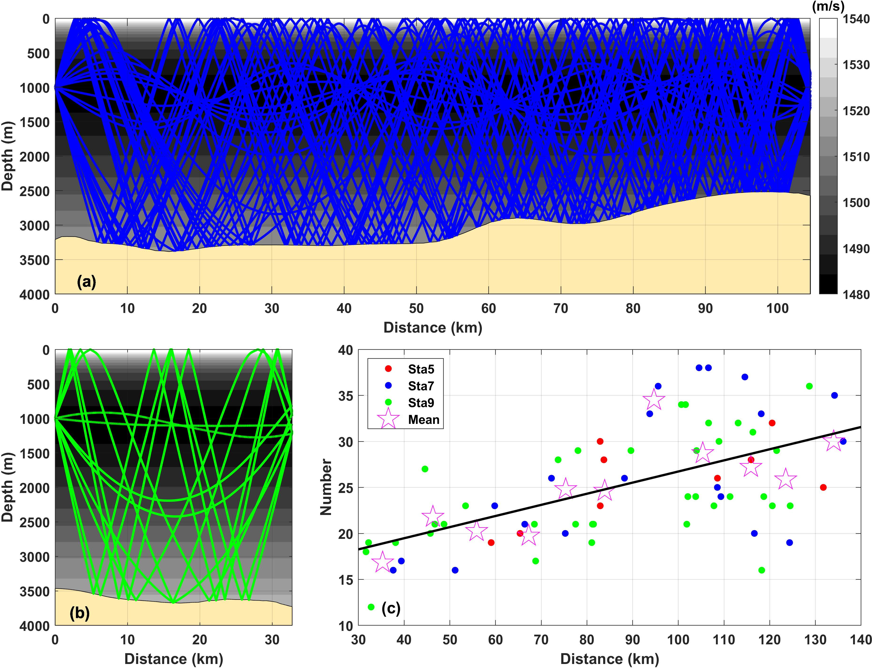
Figure 1 The typical ray pattern simulated using the Bellhop ray tracing scheme together with the reference sound speed profile. (A, B) show the typical ray patterns for L=105 km and L=33 km, respectively. The background color indicates the time- and domain-averaged reference sound speed profiles. (C) shows the number of rays plotted against the station distances. The open star marks indicated the mean of the ray number, calculated for every horizontal grid box of 10 km.
From the HYCOM reanalysis data from 1993 to 2011, we accumulated the vertical profiles of the sound speed to take seasonal averages using the daily temperature, salinity, and depth data, interpolated to 1 m interval data, and then subtracted the climatologically averaged sound speed from the daily data to obtain the deviated sound speed profiles (Figure 2A). The deviated SSP varied greatly with time and showed different vertical structures in the upper ocean in the different seasons. In the upper 200 m, the deviated sound speeds notably varied owing to the main thermocline, with a variation range of approximately ±15 m/s. The range of variation in the deviated sound speeds decreased with increasing depth. At a 1000 m depth, the variation in deviated sound speeds was only within ±2 m/s. Different seasonal profiles showed that the deviated sound speed varied within ±5 m/s in the subsurface layer, where the seasonal thermocline of the SSC was present (Wang et al., 2022). EOF decomposition was applied to the deviated sound-speed profile data, and the first six EOF modes were calculated (Figure 2B). The contribution rates of the six EOF modes were 81.7%, 12.4%, 3.5%, 1.0%, 0.9%, 0.5%, respectively, and the first three modes were the major modes accounting for the contribution rate of 97.6%. The deviated sound speed showed a large variability in the upper 400 m, and the variability diminished rapidly with depth. For the first several modes of the EOF, near-surface-intensified phenomena were also prominent in the upper 150 m, where the deviated sound speed had a large value. At depths greater than 600 m, the speed of the deviating sound decreased rapidly.
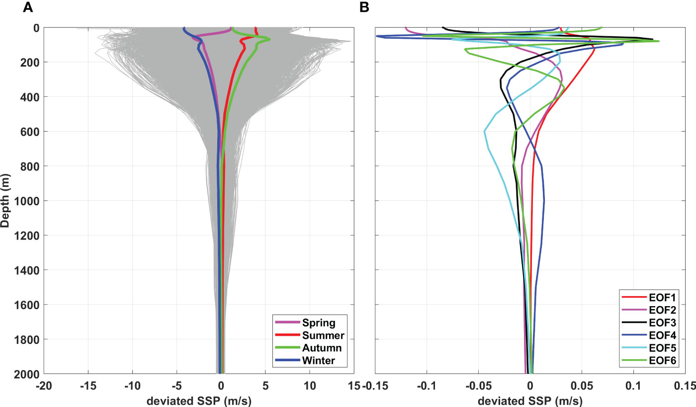
Figure 2 EOF decomposition for the deviated sound speed profiles. (A) The vertical profiles of deviated sound speed data accumulated from 1993 to 2011; (B) The vertical profiles of deviated sound speeds for the first six EOF modes.
The HYCOM reanalysis product was developed earlier and is currently the longest-time-scale high-resolution dataset with eddy-resolving resolution (Adams et al., 2011). Based on the hydrographic data (temperature and salinity) with a time resolution of 1 d and a horizontal resolution of 1/12° in the HYCOM dataset, we selected a 1° × 1° latitude-longitude model domain (approximately 104 × 111 km) in the southwest of the Luzon Strait, where the Kuroshio frequently intrudes. Mesoscale eddies that frequently appear in this area (Chen et al., 2011), where are the targets of acoustic tomography. In the analysis, the effects of station number on the accuracy of the inversion and the standard configuration of stations with asymmetry were considered. Figure 3 shows the standard configurations for the five-, seven-, and nine-station cases. The total number of rectangular grids was M=7 × 7 = 49. With an increase in the number of acoustic stations, the number of acoustic transmission lines increased exponentially. The five-, seven-, and nine-station cases constructed ten, twenty-one, and thirty-six transmission paths in the horizontal domain, respectively. The observational information, acquired from sound propagation among tomographic stations, increased with exponential growth rather than the linear growth obtained by conventional mooring stations (Zhang et al., 2017).
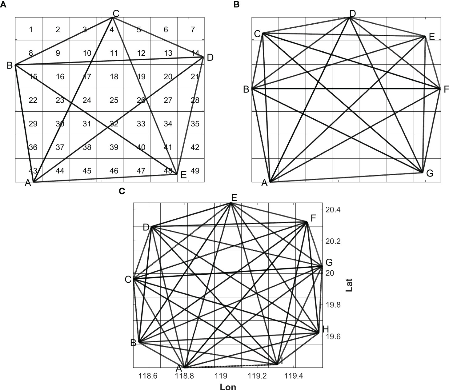
Figure 3 The standard configuration for (A) five, (B) seven, and (C) nine stations superimposed on the horizontal-slice inversion grid. The grids are numbered as 1–49; A–I are the names of the stations.
The temperature distribution on January 6, 2011, was selected with a focus on the warm eddy in the simulated domain. To facilitate comparison, the horizontal-slice distributions of the depth-averaged temperatures are shown at every 50-m depth with a 7 × 7 grid, as shown in Figure 4. In the upper layer (100–600 m), the core of temperature anomaly due to warm eddies intensified with a maximum temperature anomaly of approximately 2°C at a depth of 100–150 m. The eddies penetrated deeply, extending from 100 m to 600 m. The core of the temperature anomaly gradually weakened as depth increased, constructing an incline toward the southeast.
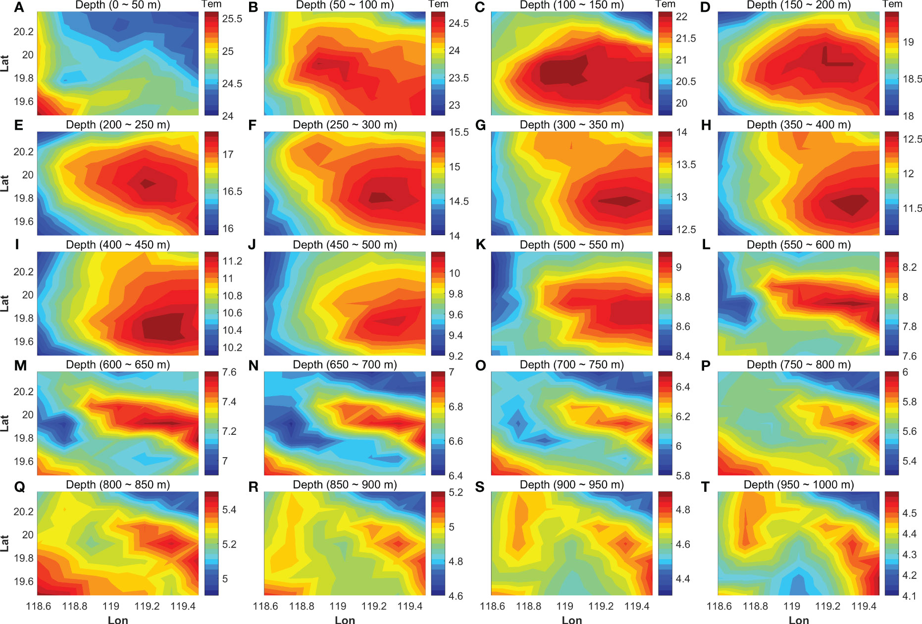
Figure 4 The horizontal-slice depth-average temperature distribution every 50 m with the 7 × 7 grid. The depth information is indicated at the top of each figure (A–T). The color bar of temperature is also indicated at the right of each figure.
The propagation of acoustic signals in the ocean can be approximated by using refracted acoustic rays. The propagation of ray paths in the vertical section depends on the vertical distribution of sound speed and velocity (Munk et al., 1995). This study focused on the influence of sound speed on propagation time without considering the velocity. The travel time deviation () for the i-th ray path traveling between the acoustic station pair is expressed as follows (Zhang et al., 2015):
When sound is transmitted from a source, it propagates in a stratified ocean; refracted rays passing through different depths are constructed, and various travel times are obtained from a receiver. For the vertical-slice inversion, the tomographic domain is decomposed into N depth layers such that the travel time deviation (Equation 1) is reduced to a discrete form as follows:
where represents the actual length of the i-th ray through the z-th layer and and represent the reference sound speed and the average sound speed deviation of the z-th layer, respectively.
The purpose of vertical-slice inversion was to reconstruct the vertical distribution of the layer-average sound speed deviations () using the travel time deviation as known variables. In this study, we considered a method in which the depth layer is decomposed into 4000 sublayers with an interval of 1 m. Because of the limited travel time information, only the sound speed deviation for typical layers was calculated (Taniguchi et al., 2013; Dai et al., 2023).
The EOF decomposition method was introduced to reduce the number of unknown inversion variables. In this study, the first six EOF modes (M=6) for the sound speed deviation were introduced. Subsequently, Equation (2) was transformed into
where is the value of the j-th EOF mode crossing the z-th layer, and is the coefficient for the j-th EOF mode. The goal of formulation is to determine the unknown variables () at every observation time when travel time deviation () is acquired. Finally, the vertical slice distribution of the average sound speed deviation was reconstructed using the following formula:
As a result of applying the EOF mode method, the number of unknown variables (the coefficient number of the EOF modes) was considerably reduced.
The tomography domain was surrounded by five, seven, and nine acoustic stations, typical cases for constructing ten, twenty-one, and thirty-six transmission paths, respectively. The horizontal-layered distribution of the sound speed deviation obtained in the vertical-slice inversion and the lengths of the transmission paths crossing individual grids were used in the horizontal-slice inversion as known variables. The formulation for the horizontal-slice inversion is represented as follows:
where is the layer-average sound speed deviation for the x-th grid at the z-th layer obtained from Equation (4), is the length of the i-th ray projected onto the z-th horizontal layer crossing the x-th grid, is the sound speed deviation of the x-th grid at the z-th layer, and is the length of the i-th projected ray at the z-th layer.
Three-dimensional mesoscale sound speed fields were reconstructed by combining the vertical and horizontal slice inversions. The simulation region was divided into a depth range of 50 m from the surface to 1000 m. To better describe mesoscale eddies, the three-dimensional distribution of sound speed was converted into a three-dimensional distribution of temperature according to the correlation formula using the sound speed deviation and taking depth as a variable. From the surface to a depth of 1000 m at an interval of 50 m, a change of 1 ms-1 in sound speed was equivalent to temperature changes of 0.5–0.2 °C.
Equations (3) and (5), which correspond to the vertical- and horizontal-slice inversions, respectively, are expressed in matrix form as follows:
where y is the simulated data set vector, x is the unknown variable vector, E is the transform matrix, and n is the noise vector.
In this study, the tapered least-squares method was adopted to obtain the optimal solution. In the tapered least squares method, we can express the objective function as follows:
where is the damping parameter. The expected solution is obtained, so that to minimize the objective function as follows:
The L-curve method developed by Hansen and O’Leary (1993) was used to determine the optimal value of . Consequently, the optimal solution of the sound speed deviation fields was obtained more flexibly than with stochastic inversion, which requires the covariance of the expected solution prior to inversion.
Figure 5 shows the horizontal-slice contour maps of temperature fields with warm eddy anomaly, reconstructed by inversion for the five-station number. The results of 20 depth averaged temperature fields at a 50 m interval from the surface to a depth of 1000 m are shown in Figures 5A–T, 6A–T, 7A–T show the contour maps of temperature for seven- and nine-station cases, respectively. The mesoscale anomaly was intensified in the depth layers of 100–600 m, as visible in the 50 m-interval depth-average temperature field (Figure 4), and rapidly diminished with depth in the layers deeper than 600 m. The core of the anomaly, which corresponded to the mesoscale eddies existing in the depth range of 50–600 m, was not clear in Figure 5 (five-station case). The cores were reconstructed with almost the same horizontal positions as Figure 4 in the depth range of 100–550 m for Figure 6 (seven-station case) and in the depth range of 150–500 m for Figure 7 (nine-station case).
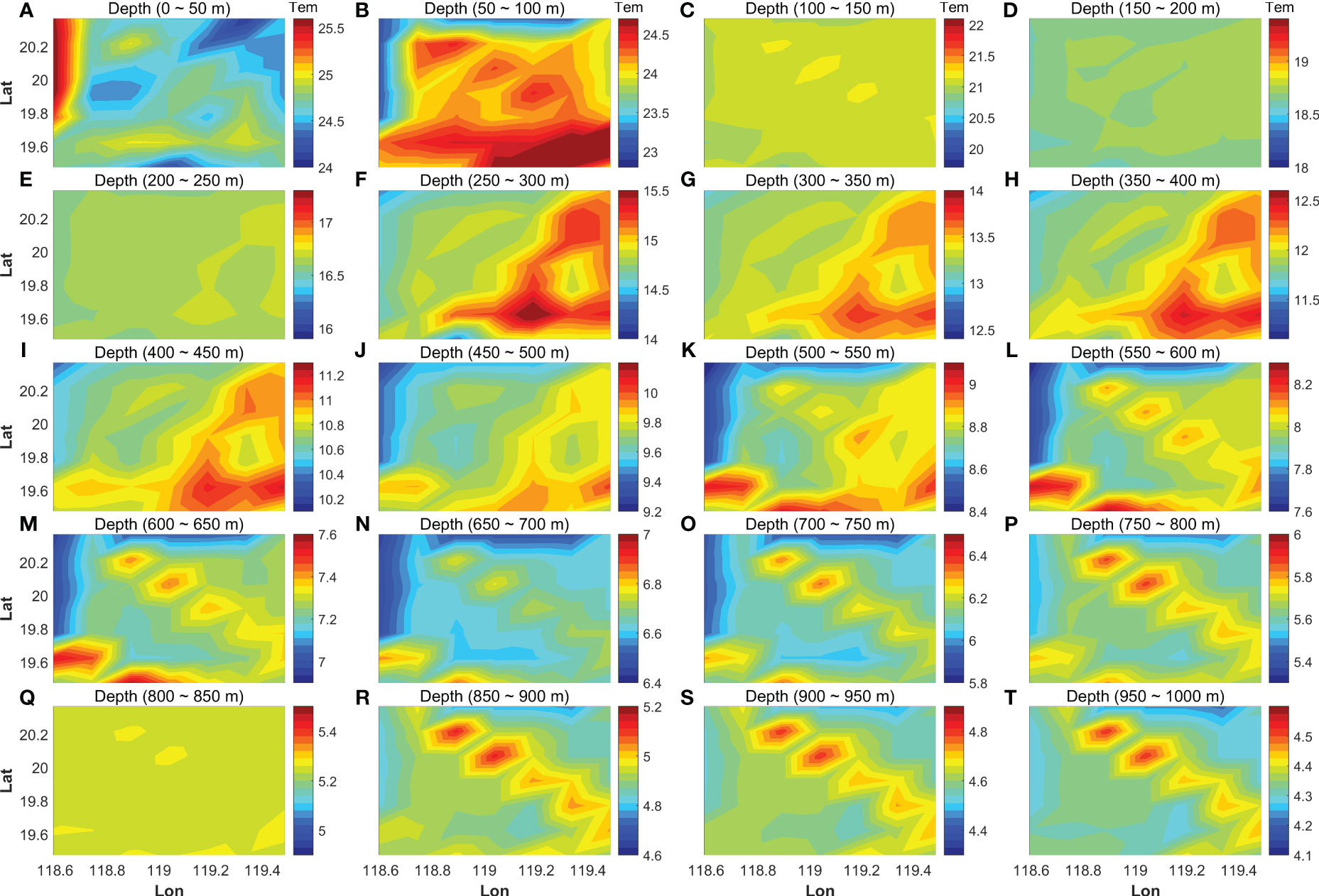
Figure 5 Contour maps of the horizontal-slice temperature fields, reconstructed for five acoustic stations. The depth range is indicated at the top of each figure (A–T). The color bar of temperature is also indicated at the right of each figure.
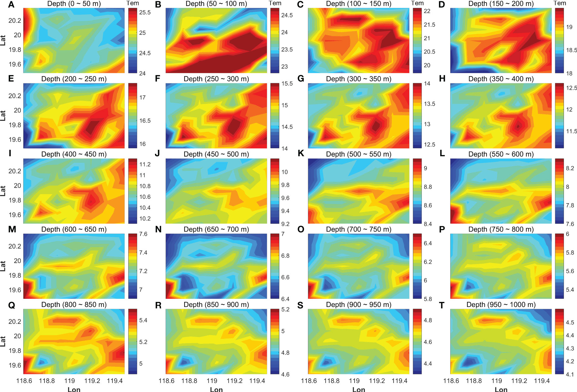
Figure 6 Contour maps of the horizontal-slice temperature fields, reconstructed for seven acoustic stations. Others are similar to Figure 5.
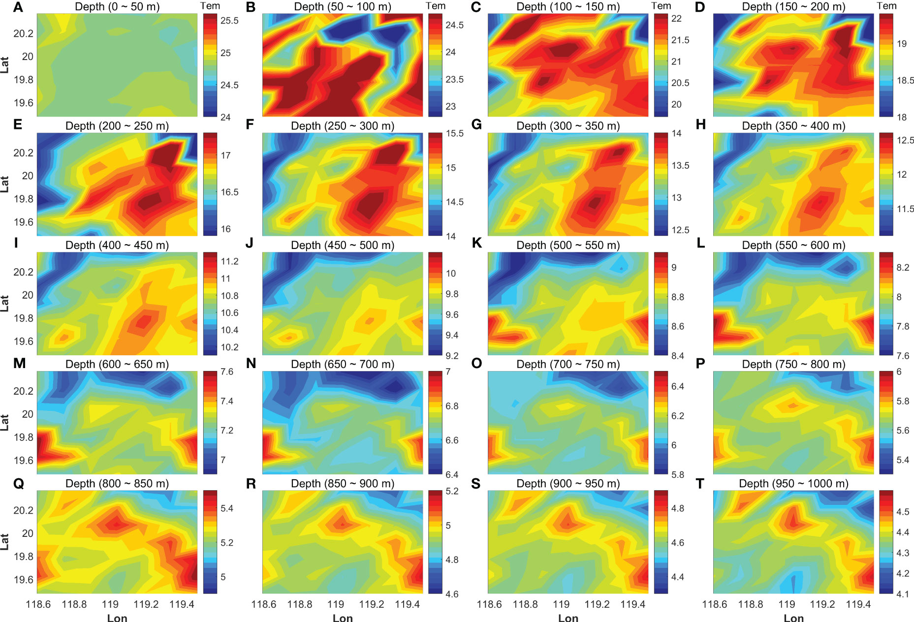
Figure 7 Contour maps of the horizontal-slice temperature fields, reconstructed for nine acoustic stations. Others are similar to Figure 5.
To evaluate the performance of the tomographic inversion, the inverted temperature at the m-th grid point of each layer was compared with the HYCOM data using two indices, CCOE and RMSD, as follows:
where is the time and and represent the HYCOM and inverted temperatures at each layer, respectively. and represent the average values of HYCOM and the inverted temperatures over all grid points in each layer, respectively.
The CCOE (Equation 9) and RMSD (Equations 10) for the HYCOM data and the inversion results averaged over the simulation domain were calculated for the three acoustic stations. Figure 8 shows the time plot of the comparison results for the entire year of 2011 in the second layer, where the sound speed (temperature) anomaly had the largest value. Within one year, the temperature varied from 20.0 °C to 26.5 °C. In general, all three sets of temporal data varied with similar tendencies. The CCOE and RMSD were 0.980 and 0.297 °C for the five-station case, 0.991 and 0.197 °C for the seven-station case, and 0.989 and 0.220 °C for the nine-station case, respectively. The RMSD was the smallest for the seven-station case, whereas the nine-station case had the highest horizontal resolution of the three cases.
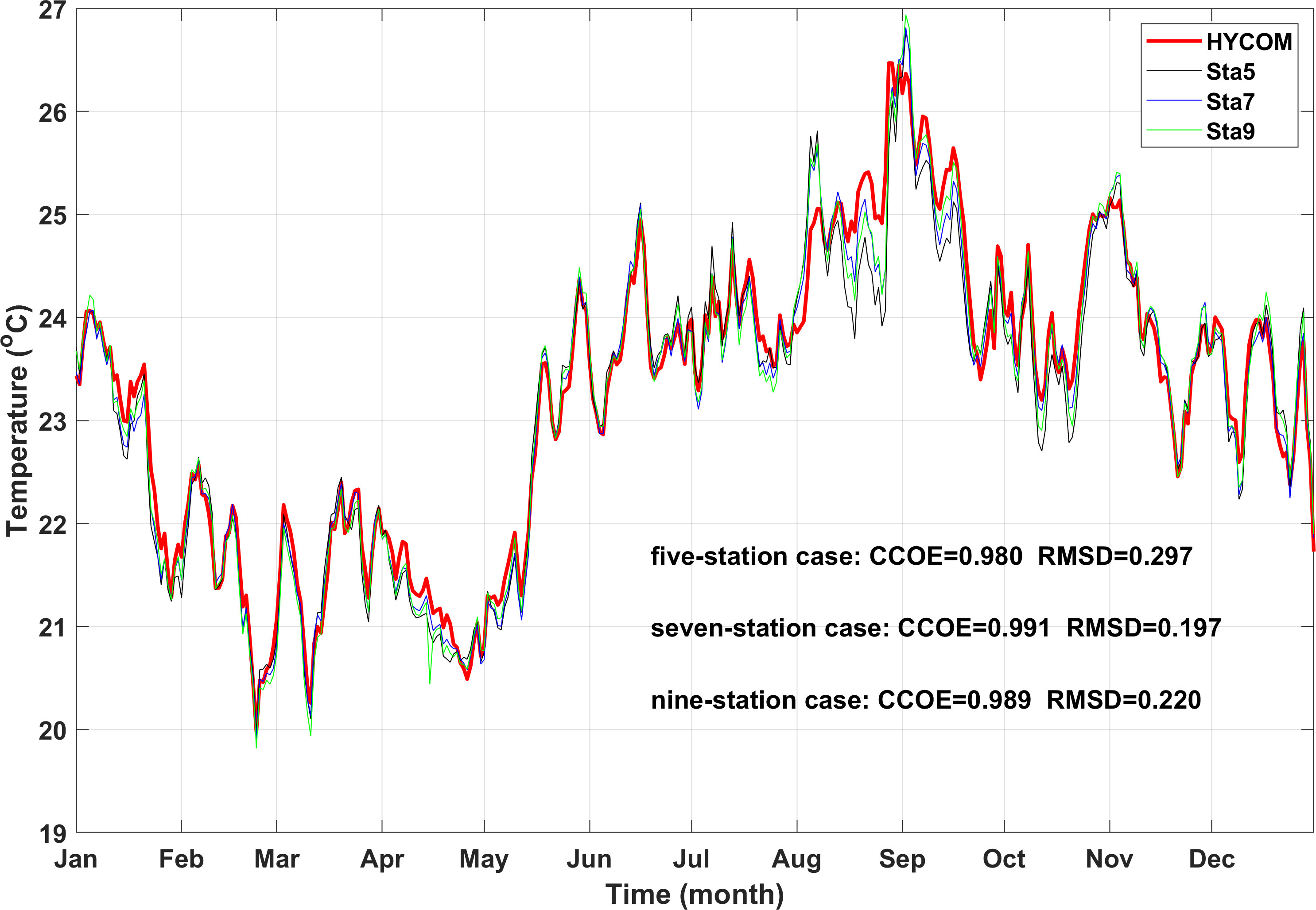
Figure 8 Time series of the 2011 HYCOM data (red line) and inversion results for five-station (black line), seven-station (blue line), and nine-station (green line) cases in the second layer. CCOE and RMSD are indicated in the lower right of the figure.
Statistical analyses of the RMSD at each layer provided an important indicator of the inversion performance. In the following analysis, the entire depth layer, from the surface to a depth of 1000 m, was divided into 20 sublayers every 50 m.
The mean and standard deviation (STD) of the RMSD were calculated for every grid of each depth layer, implying that the inversion accuracy varied with depth (Figure 9). The mean and STD of the RMSD were maximal in the second layer around the main thermocline. Its value was 0.64 °C for the five-station case, 0.55 °C for the seven-station case, and 0.78 °C for the nine-station case, showing that the seven-station case had a minimum value of mean. The results also showed that the nine-station case had the maximum value of the STD around the second layer. The mean and STD of the RMSD showed a decreasing trend with the number of depth layers. Therefore, the performance of inversion was best for the seven-station case rather than for the nine-station case, with the highest resolution of the three cases.
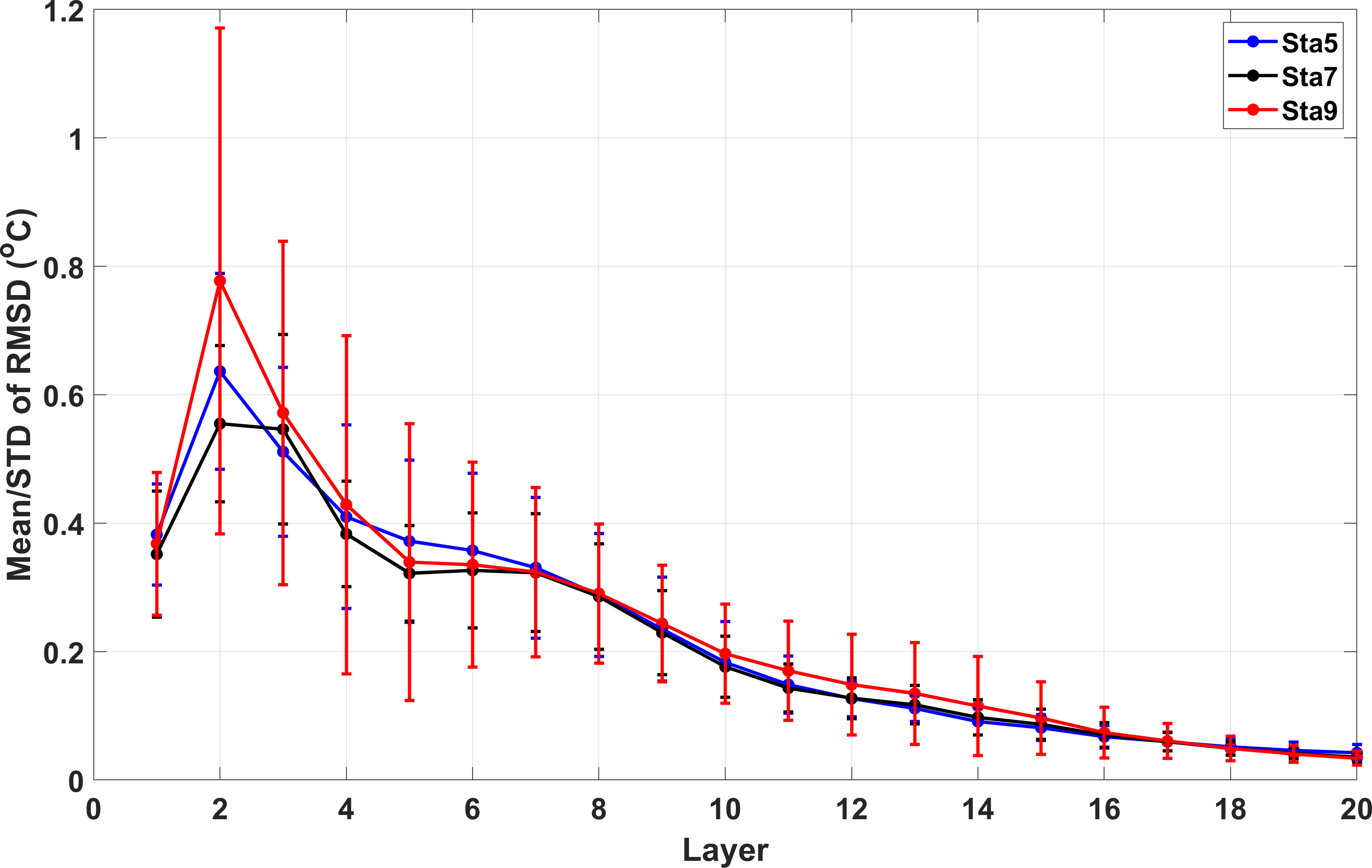
Figure 9 Layer dependence of the mean and STD of RMSD for the HYCOM and inverted data at each depth layer. The dots and vertical bars indicate the mean and STD, respectively. The results for five-, seven-, and nine-station cases are indicated with the blue, black, and red colors as simulated in the legend at the upper right of the figure.
The accuracy of horizontal-slice inversion depends on the spatial resolution (Park and Kaneko, 2001; Zhang et al., 2017). The number of stations determines the number of transmission paths required. The spatial resolution was formulated using the area (A) of the simulation domain and the number () of acoustic transmission paths, as follows:
where A = 104 × 111 km =11,544 km2. For the three station configurations on a horizontal slice, the spatial resolutions were calculated using Equation (11) and are listed in Table 1.
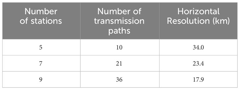
Table 1 Number of stations, number of transmission paths, and horizontal-slice spatial resolutions calculated for the three cases of station configurations.
In this study, the results for the mesoscale anomaly inversion showed that the inversion performance for the seven-station case was better than that for the nine-station case, with a higher spatial resolution. This means that the accuracy of three-dimensional inversion depends on the horizontal-slice spatial resolution as well as the vertical-slice spatial resolution. To illustrate the vertical-slice inversion performance more directly, the RMSD for the vertical-slice inverted temperature of the full water depth and HYCOM data were plotted against station distance and ray number (Figure 10). When the distance between stations increased from 30 km to 100 km, the RMSD for the vertical-slice inversion significantly decreased with increasing distances. For distances greater than 100 km, the RMSD was approximately constant (Figure 10A). Similarly, the RMSD for the vertical-slice inversion decreased as the number of acoustic rays increased (Figure 10B). With increasing distance, oceanic signals with smaller length scales were filtered out, increasing the smoothness of the inversion. In addition, the larger the number of refracted rays, the smaller the shadow zone, resulting in a higher vertical-slice resolution. The RMSD was close to a constant value for ray numbers greater than 30. The RMSD of the vertical slice was larger due to the small distance between station pairs of the nine-station case. However, the RMSD was more balanced due to the more appropriate distances in the seven-station case. Significantly, the comparison of temperature profiles from the vertical-slice inversion and HYCOM results for different station configurations during mesoscale eddy period is presented in Supplementary Figure S1 of the Supplementary material.
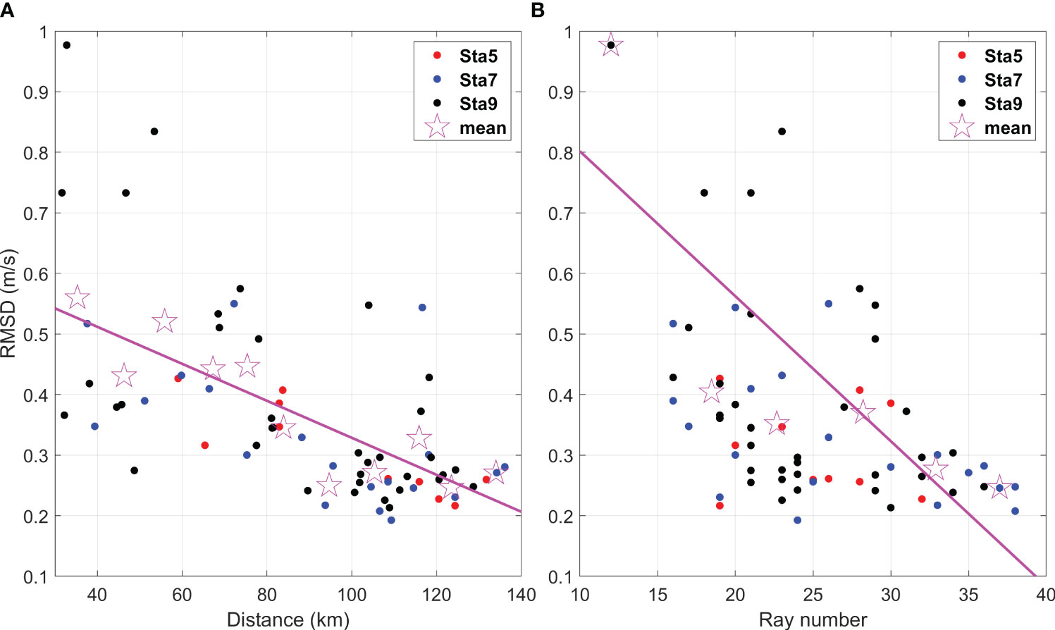
Figure 10 RMSDs for the inverted and HYCOM temperatures, plotted against (A) the station distance and (B) the ray number. The pink straight line is the regression line in each figure. The open star marks indicate the mean value of RMSD calculated for every horizontal grid box of 10 km and five rays, respectively.
Mesoscale eddies are difficult to measure synchronously using conventional shipboard methods because their horizontal scales are greater than 100 km. This can be achieved through acoustic tomography methods using a network of multiple acoustic stations located at the periphery of the observation domain. By simulating the OAT experiment using HYCOM reanalysis data, we tested three types of OAT station configurations: five, seven, and nine acoustic stations located at the periphery of a 104 × 111 km domain. The simulation fields were in the northern SCS, with mesoscale eddies generated due to the intrusion of the Kuroshio through the Luzon Strait.
A new inversion method was proposed by combining the EOF method in a vertical slice and the grid-segmented method in a horizontal slice. The tapered least-squares method combined with the L-curve method was used in the inversion process. The performance of the inversion was evaluated for the three cases of five, seven, and nine stations using the correlation coefficient (CCOE) and root mean square difference (RMSD) for the inverted and HYCOM reanalysis data. For a 100 × 100 km domain, the seven-station case provided an optimal number to reconstruct the mesoscale eddy phenomena rather than the nine-station case, with the highest horizontal resolution of the three cases. This means that the accuracy of the three-dimensional inversion depends on the horizontal-slice spatial resolution as well as the vertical-slice spatial resolution. Furthermore, the horizontal-slice spatial resolution, ray number, and station distance affect the vertical-slice inversion accuracy. The fewer the number of refracted rays, the greater the shadow zone. A longer station distance smoothens out oceanic phenomena at smaller scales.
In this study, we proposed ocean acoustic tomography as an underwater remote sensing technique that is fully capable of observing mesoscale eddies.
The HYCOM reanalysis data can be downloaded online (https://hycom.org/dataserver/gofs-3pt0/reanalysis). The original contributions presented in the study are included in the article/Supplementary Material. Further inquiries can be directed to the corresponding author.
CZ: Conceptualization, Methodology, Visualization, Writing – original draft, Writing – review & editing. Z-NZ: Methodology, Writing – review & editing. CX: Methodology, Writing – review & editing. X-HZ: Conceptualization, Writing – review & editing. Z-JL: Writing – review & editing.
The author(s) declare financial support was received for the research, authorship, and/or publication of this article. This study was sponsored by the National Key Research and Development Program of China (2021YFC3101502), the National Natural Science Foundation of China (Grants 41920104006, 41976001 and 52071293), the Scientific Research Fund of Second Institute of Oceanography, MNR (Grant JZ2001), Zhejiang Provincial Natural Science Foundation of China (LY24D060002), and the Innovation Group Project of Southern Marine Science and Engineering Guangdong Laboratory (Zhuhai) (311020004).
The authors declare that the research was conducted in the absence of any commercial or financial relationships that could be construed as a potential conflict of interest.
All claims expressed in this article are solely those of the authors and do not necessarily represent those of their affiliated organizations, or those of the publisher, the editors and the reviewers. Any product that may be evaluated in this article, or claim that may be made by its manufacturer, is not guaranteed or endorsed by the publisher.
The Supplementary Material for this article can be found online at: https://www.frontiersin.org/articles/10.3389/fmars.2024.1350337/full#supplementary-material
Adams D. K., McGillicuddy D. J., Zamudio L., Thurnherr A. M., Liang X., Rouxel O., et al. (2011). Surface-generated mesoscale eddies transport deep-sea products from hydrothermal vents. Science 332, 580–583. doi: 10.1126/science.1201066
Chen G., Hou Y., Chu X. (2011). Mesoscale eddies in the South China Sea: Mean properties, spatiotemporal variability, and impact on thermohaline structure. J. Geophys. Res. 116, 102–108. doi: 10.1029/2010JC006716
Chu X., Chen G., Qi Y. (2020). Periodic mesoscale eddies in the South China sea. J. Geophys. Res. Ocean 125, e2019JC015139. doi: 10.1029/2019JC015139
Cornuelle B., Wunsch C., Behringer D., Birdsall T., Brown M., Heinmiller R., et al. (1985). Tomographic maps of the ocean mesoscale. Part 1: pure acoustics. J. Phys. Oceanogr. 15, 133–152. doi: 10.1175/1520-0485(1985)015<0133:TMOTOM>2.0.CO;2
Dai L., Xiao C., Zhu X.-H., Zhu Z.-N., Zhang C., Zheng H., et al. (2023). Tomographic reconstruction of 3D sound speed fields to reveal internal tides on the continental slope of the South China Sea. Front. Mar. Sci. 9. doi: 10.3389/fmars.2022.1107184
Fukumori I., Wunsch C. (1991). Efficient representation of the North Atlantic hydrographic and chemical distributions. Prog. Oceanogr 27, 111–195. doi: 10.1016/0079-6611(91)90015-E
Hansen P., O’Leary D. P. (1993). The use of the L-curve in the regularization of discrete ill-posed problems. Siam J. Sci. Comput. 14 (6), 1487–1503. doi: 10.1137/0914086
Howe B. M., Worceser P. F., Spindel R. C. (1987). Ocean acoustic tomography: mesoscale velocity. J. Geophys. Res. 92, 3785–3805. doi: 10.1029/JC092iC04p03785
Kaneko A., Zhu X.-H., Ju Lin J. (2020). Coastal Acoustic Tomography (Amsterdam, Netherlands: Elsevier). doi: 10.1016/B978-0-12-818507-0.00003-2
LeBlanc L., Middleton F. H. (1980). An underwater acoustic sound velocity data model. J. Acoust. Soc Am. 67, 2055–2062. doi: 10.1121/1.384448
Liu Q., Kaneko A., Su J. (2008). Recent progress in studies of the South China Sea circulation. J. Oceano. 64, 753–762. doi: 10.1007/s10872-008-0063-8
MacKenzie K. V. (1981). Nine-term equation for sound speed in the ocean. J. Acoust. Soc Am. 70, 807–812. doi: 10.1121/1.386920
Munk W., Worceser P. F., Wunsch C. (1995). Ocean acoustic tomography (Cambridge: Cambridge Univ. Press). 433. doi: 10.1017/CBO9780511666926
Munk W., Wunsch C. (1979). Ocean acoustic tomography: a scheme for large scale monitoring. Deep-Sea Res. 26A, 123–161. doi: 10.1016/0198-0149(79)90073-6
Nan F., He Z., Zhou H., Wang D. (2011). Three long-lived anticyclonic eddies in the northern South China Sea. J. Geophys. Res. 116, C05002. doi: 10.1029/2010JC006790
Park Y., Jeon C., Song H., Choi Y., Chae J.-Y., Lee E.-J., et al. (2021). Novel method for the estimation of vertical temperature profiles using a coastal acoustic tomography system. Front. Mar. Sci. 8. doi: 10.3389/fmars.2021.675456
Park J.-H., Kaneko A. (2001). Computer simulation of the coastal acoustic tomography by a two-dimensional vortex mode. J. Oceangr. 57, 593–602. doi: 10.1023/A:1021211820885
Syamsudin F., Taniguchi N., Zhang C., Hanifa A. D., Li G., Chen M., et al. (2019). Observing internal solitary waves in the Lombok Strait by coastal acoustic tomography. Geophys. Res. Lett. 46, 10475–10483. doi: 10.1029/2019GL084595
Taniguchi N., Huang C., Kaneko A., Liu C., Howe B. M., Wang Y., et al. (2013). Measuring the Kuroshio Current with ocean acoustic tomography. J. Acoust. Soc Am. 134, 3272–3281. doi: 10.1121/1.4818842
Wang X., Du Y., Zhang Y., Wang T., Wang Mi., Jing Z. (2022). Subsurface anticyclonic eddy transited from Kuroshio shedding eddy in the northern South China Sea. J. Phys. Oceanogr. 53 (3), 841–861. doi: 10.1175/JPO-D-22-0106.1
Wang G., Su J., Chu P. C. (2003). Mesoscale eddies in the South China Sea observed with altimeter data. Geophys. Res. Lett. 30, 2121–1226. doi: 10.1029/2003GL018532
Wang D., Xu H., Lin J., Hu J. (2008). Anticyclonic eddies in the northeastern South China Sea during winter 2003/2004. J. Oceangr. 64 (6), 925–936. doi: 10.1007/s10872-008-0076-3
Yuan G., Nakano I., Fujimori H., Nakamura T., Kamoshida T., Kaya A. (1999). Tomographic measurements of the Kuroshio Extension meander and its associated eddies. Geophys. Res. Lett. 26, 79–82. doi: 10.1029/1998GL900253
Zhang C., Kaneko A., Zhu X.-H., Gohda N. (2015). Tomographic mapping of a coastal upwelling and the associated diurnal internal tides in Hiroshima Bay, Japan. J. Geophys. Res.Oceans 120, 4288–4305. doi: 10.1002/2014JC010676
Zhang C., Zhu X.-H., Zhu Z.-N., Liu W., Zhang Z.-Z., Fan X.-P., et al. (2017). High-precision measurement of tidal current structures using coastal acoustic tomography. Estuar. Coast. Shelf Sci. 193, 12–24. doi: 10.1016/j.ecss.2017.05.014
Zheng H., Gohda N., Noguchi H., Ito T., Yamaoko H., Tamura T., et al. (1997). Reciprocal sound transmission experiment for current measurement in the Seto Inland Sea, Japan. J. Oceanogr. 53, 117–127.
Zhu X.-H., Kanko A., Wu Q.-S., Zhang C., Taniguchi N., Gohda N. (2013). Mapping tidal current structures in zhitouyang bay, China, using coastal acoustic tomography. IEEE J. Oceanic Eng. 38, 285–296. doi: 10.1109/JOE.2012.2223911
Keywords: ocean acoustic tomography, inversion of three-dimensional temperature fields, mesoscale phenomena, HYCOM data, South China Sea
Citation: Zhang C, Zhu Z-N, Xiao C, Zhu X-H and Liu Z-J (2024) Acoustic tomographic inversion of 3D temperature fields with mesoscale anomaly in the South China Sea. Front. Mar. Sci. 11:1350337. doi: 10.3389/fmars.2024.1350337
Received: 05 December 2023; Accepted: 05 February 2024;
Published: 22 February 2024.
Edited by:
Arata Kaneko, Hiroshima University, JapanReviewed by:
Chanhyung Jeon, Pusan National University, Republic of KoreaCopyright © 2024 Zhang, Zhu, Xiao, Zhu and Liu. This is an open-access article distributed under the terms of the Creative Commons Attribution License (CC BY). The use, distribution or reproduction in other forums is permitted, provided the original author(s) and the copyright owner(s) are credited and that the original publication in this journal is cited, in accordance with accepted academic practice. No use, distribution or reproduction is permitted which does not comply with these terms.
*Correspondence: Xiao-Hua Zhu, eGh6aHVAc2lvLm9yZy5jbg==
Disclaimer: All claims expressed in this article are solely those of the authors and do not necessarily represent those of their affiliated organizations, or those of the publisher, the editors and the reviewers. Any product that may be evaluated in this article or claim that may be made by its manufacturer is not guaranteed or endorsed by the publisher.
Research integrity at Frontiers
Learn more about the work of our research integrity team to safeguard the quality of each article we publish.