
95% of researchers rate our articles as excellent or good
Learn more about the work of our research integrity team to safeguard the quality of each article we publish.
Find out more
ORIGINAL RESEARCH article
Front. Mar. Sci. , 20 February 2024
Sec. Marine Conservation and Sustainability
Volume 11 - 2024 | https://doi.org/10.3389/fmars.2024.1344013
This article is part of the Research Topic Assessing and Limiting the Adverse Effects of Offshore Wind Farm Development on Seabirds and Marine Mammals View all 6 articles
 Auriane Virgili1,2*
 Sophie Laran1
 Matthieu Authier1
 Ghislain Dorémus1
 Olivier Van Canneyt1
 Jérôme Spitz1,3
Intense development of Offshore Wind Farms (OWFs) has occurred in the North Sea with several more farms planned for the near future. These OWFs pose a threat to marine megafauna stressing the need to mitigate the impact of human activities. To help mitigate impacts, the Before After Gradient (BAG) design was proposed. We explored the use of the BAG method on megafauna sightings recorded at different distances from OWFs in the southern North Sea. We predicted intra-annual variability in species distribution, then correlated species distribution with the presence of operational OWFs and investigated the potential impact the operation of prospective OWFs may have on species distribution. Four patterns of intra-annual variability were predicted: species most abundant in spring, in winter, in both spring and winter, or all year round. We recommend that future OWF constructions be planned in summer and early fall to minimise impact on cetaceans and that offshore areas off northern France and Belgium be avoided to minimise impact on seabirds. Our prospective analysis predicted a decreased density for most species with the operation of prospective OWFs. Prospective approaches, using e.g. a BAG design, are paramount to inform species conservation as they can forecast the likely responses of megafauna to anthropogenic disturbances.
Anthropogenic activity in the southern region of the North Sea is among the most intense in the world. A strongly used shipping lane crosses the Dover Strait and the Belgian and British waters are used for intense fisheries as well as for offshore wind farm construction (Halpern et al., 2008). There has been a marked increase in marine renewable energy projects in the southern North Sea in recent years, particularly in offshore wind farms (OWFs), the number of which is expected to more than double in the coming years (European Commission, 2023). The development of these OWFs pose various threats to marine megafauna (i.e. marine mammals, seabirds, large fish and marine turtles) living in and travelling through the area, including: (1) direct mortalities due to collisions between seabirds and wind turbines (Drewitt and Langston, 2006); (2) physiological stress, such as lesions and hearing loss due to pile driving (Tougaard et al., 2004; Board and National Research Council, 2005; Thomsen et al., 2006; Dähne et al., 2013); and (3) disturbances due to pile driving and intense marine traffic, which can induce changes in distribution, behaviour, reproduction or foraging activity patterns, e.g. by displacing individuals from suitable habitats (Drewitt and Langston, 2006; Brandt et al., 2011; Bergström et al., 2014; Vallejo et al., 2017; Mendel et al., 2019). Harbour porpoises (Phocoena phocoena) and various seabird species (e.g. northern gannets Morus bassanus, northern fulmars Fulmarus glacialis) occur in high densities in the southern part of the North Sea (Lambert et al., 2017) and are therefore significantly at risk of being affected by the spread of wind farms. It is important that we understand the threats that anthropogenic developments and activities pose to marine biodiversity to allow development of specific recommendations to mitigate them. This is the aim of the EU’s Directive 2014/89/EU, which calls for efficient marine spatial planning in European waters (Douvere, 2008; European Parliament and Council Directive 2014/89/EU).
The mitigation of threats to biodiversity comprises four sequential steps, based on the mitigation hierarchy, namely: (1) avoidance, (2) minimisation, (3) restoration and (4) offsetting (Kiesecker et al., 2010). Avoidance involves taking measures to prevent impacts (e.g. excluding breeding areas in prospective development plans). Minimisation measures reduce the duration, intensity and extent of impacts that cannot be avoided (e.g. making technological adjustments to reduce noise). When impacts cannot be completely avoided or minimised, restoration efforts aim to return an ecosystem to a pre-impact state. After the implementation of the first three steps, any residual impacts can be offset - or compensated for - in order to balance the detrimental effects with positive effects (e.g. preventing future habitat degradation; Kiesecker et al., 2010).
Avoidance is the relatively easiest and most effective step, particularly in the context of wind farming. It requires that the initial state of the biodiversity in the prospected area be thoroughly investigated in order to assess when the construction phase would have the least impact on species and where the wind farm should be established to minimise impacts during the operational phase. This assessment critically hinges on accurate knowledge of species distributions, particularly on a seasonal and monthly scale (Foley et al., 2010; Santos et al., 2019). Knowledge of the monthly distribution of marine megafauna is essential in a marine spatial planning context because these animals are highly mobile and their distributions change depending on their life cycle. Animals are particularly sensitive to disturbance during certain life stages, e.g. during mating or breeding seasons, therefore accurate seasonal and monthly distribution patterns are necessary in order to reduce the spatial and/or temporal overlap between any disruptive activities and the sensitive stages or with key aggregation areas of the species (Gilles et al., 2011; Whitt et al., 2013; Pitchford et al., 2016).
The Before After Control Impact (BACI) method (Green, 1979), consisting in comparing an impact location (e.g. a wind farm) to a control location (unaffected by humans) before and after the human intervention, is often used to meet avoidance objectives and to study the effect of offshore wind farm on species (Bergström et al., 2013; Degraer et al., 2018; Wilber et al., 2018). However, this method has limitations (e.g. difficulty in finding a suitable control location, assumption that all wind farms are equivalent) and Methratta (2020) has proposed to integrate an alternative approach into fisheries surveys, the Before After Gradient (BAG) design, to overcome these limitations. Sampling before and after construction is carried out along a spatial gradient at increasing distances from the wind farms. She performed statistical analysis such as generalised linear or additive models, using the distance to wind farms as the main explanatory variable. Relationships between samples and distance to wind farms were obtained before and after wind farm construction. In our study, we explored the use of this BAG method on seabird and harbour porpoise sightings recorded at different distances from two wind farms in the southern North Sea. According to Marques et al. (2021), only 7% of studies have used the BAG design for the assessment of seabird displacement due to OWF construction.
We conducted six aerial surveys in the southern North Sea (from 50.8 to 52°N and from 1 to 3.5°E) between April 2017 and May 2018, allowing regular monitoring over a whole year so that we could study the intra-annual variability in the distribution and abundance of marine megafauna. This area is known to be a migration corridor for various seabirds (Stienen et al., 2007). According to the BAG framework, we used density surface models to (1) predict the monthly distribution and abundance of species (Guisan and Thuiller, 2005) and (2) to correlate species distributions with the distance to two operational OWFs in the area. Based on this empirical correlation, we (3) investigated the potential impact the operation of prospective OWFs may have on species distribution, on a monthly basis. These prospective OWFs are projects currently in concept or authorised for construction but for which construction has not yet begun (https://www.4coffshore.com/offshorewind/). As suggested by Methratta (2020), our aim was to use the distance to operational OWFs as predictor in the models to establish relationships and then use these relationships to assess how species distribution would change if OWFs currently approved were implemented and fully operational in the area. Finally, we used our results, particularly the seasonal and spatial distributions obtained, to make recommendations about avoidance and minimisation measures according to Kiesecker et al. (2010). We did not assess scenarios of noise or impact reduction during the construction phase of an OWF (Interim Population Consequences of Disturbance - iPCoD model; King et al., 2015; Degraer et al., 2018) nor assess the cumulative noise impact of the construction of multiple OWFs (Disturbance Effects of Noise on the Harbour Porpoise Population in the North Sea - DEPONS model, Nabe-Nielsen et al., 2018).
A good understanding of the current monthly species distributions and the potential impacts of the increasing wind farm activity in the future will allow for clear guidelines and recommendations defining when and where wind farm construction would have the least harmful impact ecologically and will facilitate the effective mitigation and management of marine activities in the area.
We focused on six species or species groups in this study, namely: the harbour porpoise (Phocoena phocoena), auks (Uria aalge and Alca torda), the black-legged kittiwake (Rissa tridactyla), cormorants (Phalacrocorax carbo and Phalacrocorax aristotelis), the northern fulmar (Fulmarus glacialis) and the northern gannet (Morus bassanus; Table 1). Only harbour porpoises and the seabirds listed above were present in numbers adequate for analysis. Harbour porpoises, black-legged kittiwakes, northern gannets and northern fulmars could be clearly identified from the aircraft and analyses could be conducted at the species level. Cormorants and auks needed to be considered as groups based on taxonomic and morphological criteria (Table 1).
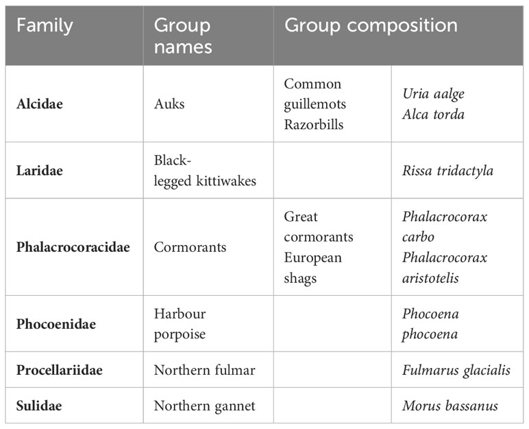
Table 1 Composition of species groups.
The study area covered about 9,400 km² and included the Belgian waters and parts of the French and English waters in the North Sea (from 50.75 to 52°N and from 1 to 3.5°E; Figure 1). Aerial visual surveys were conducted in 2017 on April 6-7, June 13-14, August 7-8, and December 4-5, and in 2018 on March 5-7 and May, 4-5. Transects were flown using high-wing aircrafts equipped with bubble windows at a target altitude of 182 m (600 feet) and a speed of 167 km.h−1 (90 knots). During the various flight sessions, two offshore wind farms, operational since 2009 and 2010, were regularly flown over, the Thanet wind farm, off the east end of Kent (England) and the Thorntonbank wind farm between the Belgian and Dutch waters (Figure 1).
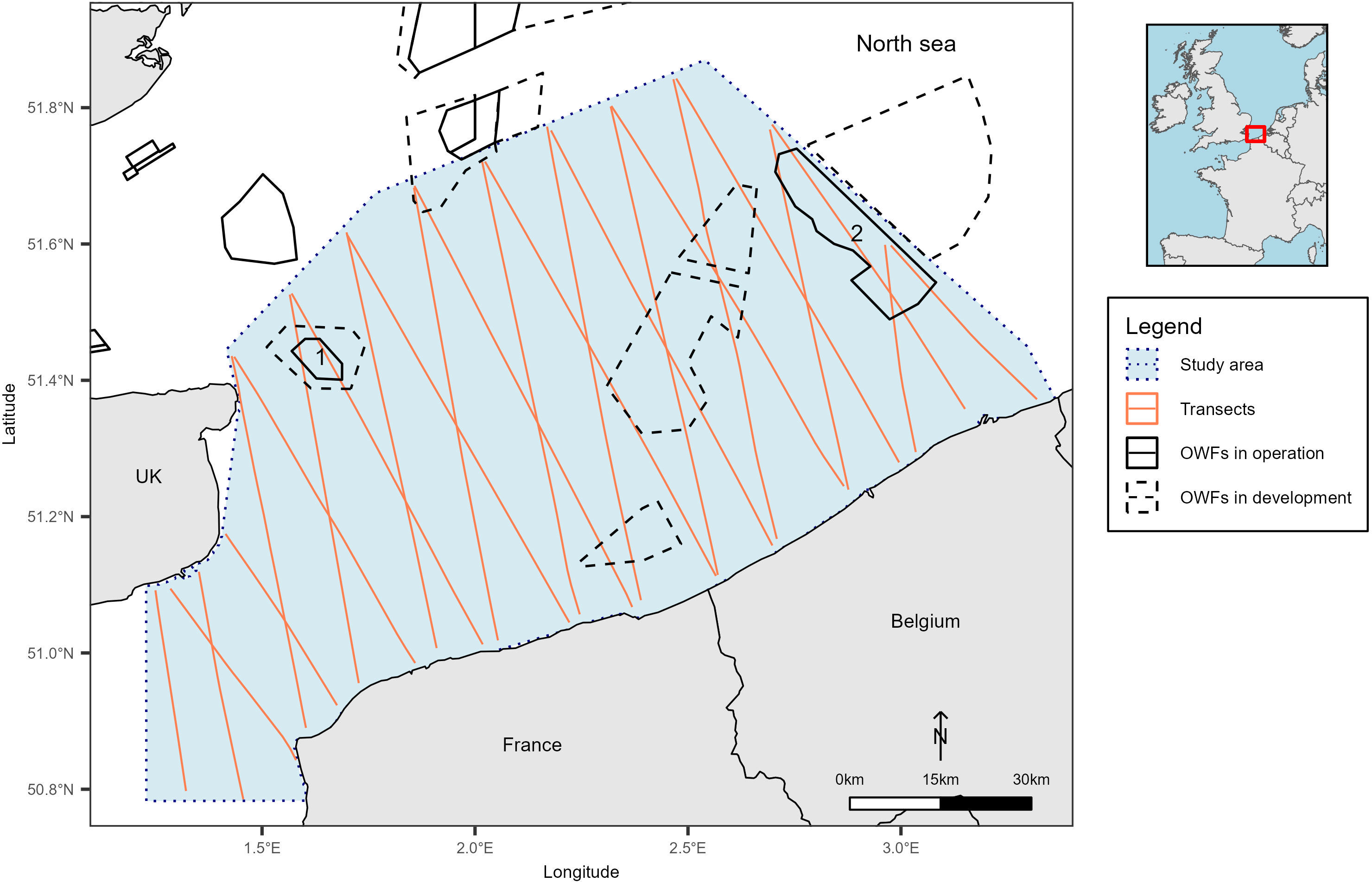
Figure 1 Study area and sampling plan. The dotted blue box delineates the study area, solid orange lines represent the sampling plan (for monthly detail refer to Appendix A), solid black boxes represent the OWFs in operation and dashed black boxes the OWFs in development. OWFs, Offshore Wind Farms; UK, United Kingdom; 1, Thanet OWF; 2, Thorntonbank OWF.
We used a multi-target protocol (described in detail in Lambert et al., 2019) to simultaneously record harbour porpoise and seabird sightings. Sightings of seabirds were recorded within a 200 m strip on each side of the aircraft (strip transect protocol), while for marine mammals, the perpendicular distance to the transect was recorded for distance sampling analyses (line transect protocol; Buckland et al., 2001). Linear transects were designed using the equal spaced zig-zag option of the software ‘Distance’ version 6.2 (Buckland et al., 2001; Thomas et al., 2010). This design can produce an unequal coverage probability when study regions are non-rectangular (Strindberg and Buckland, 2004) and this is why we used density surface modelling. This model-based approach relaxes the equal sampling probability assumption of conventional distance sampling by incorporating spatially explicit covariates to obtain a fine-grained density surface in the study area (Miller et al., 2013). Sightings and observation conditions were recorded using the ‘SAMMOA 1.0.4’ software (SAMMOA 1.0.4.; http://www.observatoire-pelagis.cnrs.fr/publications/les-outils/article/logiciel-sammoa). Observation conditions (Beaufort sea state, turbidity, cloud cover, glare severity and subjective observation conditions) were recorded at the beginning of each transect and when any condition changed. The last parameter corresponded to a subjective assessment of the detection conditions by the observer by combining all the observation conditions from poor to medium, good and excellent conditions.
Datasets were prepared for analyses using the ‘Marine Geospatial Ecology Tools’ package for ‘ArcGIS 10.3’ (Roberts et al., 2010; ESRI, 2016). Effort data were linearised and segmented into 2.5 km segments of homogenous observation conditions. Only segments recorded with good observation conditions were kept for analysis (i.e. Beaufort sea-state between 0 and 3 and subjective observation conditions from medium to excellent).
Density surface models (DSM; Miller et al., 2013) allowed us to investigate the relationships between species and their environment and predict their distributions. To do this we included both static and dynamic environmental variables, considered as potential drivers of prey availability.
Environmental variables were described by two subsets, the static and dynamic variables (Table 2). Static variables included distance to the coast, the minimum Euclidian distance to the OWFs, and for seabirds, the distance to the closest breeding colony. All distances were calculated in ArcGIS 10.3 (ESRI, 2016). Two types of OWFs were included in the analysis: 1) operational OWFs, from which the effect on species distributions were quantified (http://www.marineatlas.be/en/data for the Belgian OWF and https://www.thecrownestate.co.uk/en-gb/resources/maps-and-gis-data/ for the English OWF); and 2) OWFs in development – planned farms for which construction had not yet begun (https://www.4coffshore.com/offshorewind/) - which were used for the prospective analysis. Colonies were mapped for each seabird group (Legroux et al., 2017; Appendix B) and the strait-line distance between the centre of each segment and the nearest colony was calculated (allowing the seabirds to hypothetically fly over the mainland).
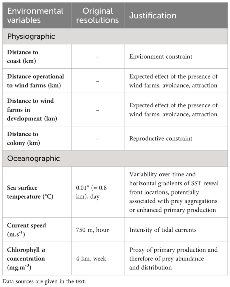
Table 2 Candidate environmental variables used for modelling density surfaces.
We also included a residual and time-varying spatial effect in the models to account for spatial autocorrelation (Wikle and Royle, 2002; see Supplementary Material in Appendix C for details). This spatial effect can be interpreted as the effect of environmental covariates not included in the models, but implies that predictions were restricted to the study area.
For dynamic variables, we used a 28-day temporal resolution (i.e. variables were averaged over the 28 days, or 4 weeks, prior the surveyed day) to account for a time lag between an environmental change and the response of marine megafauna to this new condition (Lambert et al., 2017). Environmental variables were averaged over a 2.5 × 2.5 km grid to match the 2.5 km segment length. Dynamic variables included sea surface temperature (extracted from NASA data, https://podaac.jpl.nasa.gov/dataset/JPL_OUROCEAN-L4UHfnd-GLOB-G1SST), maximum current speed (extracted from IFREMER’s MARS 2D model, https://marc.ifremer.fr/resultats/) and chlorophyll a concentration (extracted from IFREMER’s ECOMARS 3D model, https://marc.ifremer.fr/resultats/). Sea surface temperature served as a proxy for the location of fronts in which prey are concentrated. Maximum current speed was included because the English Channel and the southern North Sea are characterised by intense tidal currents. Chlorophyll a concentration served as an indicator of prey distribution. Sea surface temperatures were obtained from satellite data while other variables were derived from predictions of oceanographic models. These models were particularly useful in the case of chlorophyll a concentration because satellite data were unavailable in winter due to cloud coverage. Appendix D shows the average situation of each environmental covariate.
All environmental variables were standardised (mean-centred and divided by one standard deviation) prior to model fitting and then back-transformed to the original scale for ease of interpretation.
To model the relationships between the number of individuals (response variable) and the environment (predictors), we used generalised additive models (GAMs; Hastie and Tibshirani, 1986; Wood, 2006), assuming a binomial negative likelihood to account for data over-dispersion (Gilles et al., 2016; Isaac et al., 2019). GAMs are extensions of generalised linear models (GLMs) that allow for nonlinear relations between the response variable and predictors. It is important to note that the density surface models we built allowed for seasonal effects in both the intercepts and nonlinear relationships with the environment to predict monthly distributions. This effect was assumed to be temporally correlated: for example, the average density in January 2018 was correlated with the average density in December 2017 and February 2018 but not with the average density in August 2017 or 2018. An interaction with the month of the survey was included in the smoothing functions so that relationships with the environment can vary by month. This allowed us to obtain monthly relationships and then predict monthly distributions even if some months were not sampled during the surveys (see Appendix C for a detailed model description).
We fitted a GAM for each species group and used a model selection procedure to select the best model. To avoid collinearity between variables, we first excluded combinations of variables with Pearson correlation coefficients greater than | 0.7 | (Dormann et al., 2013). Fitted models always included the “Distance to operational wind farms “ for harbour porpoises and the “Distance to operational wind farms” and “Distance to colony” for seabirds to estimate the relationship between the number of individuals and the distance to the operational OWFs, and to assess the effect of distance to colonies on seabird distribution. This systematic inclusion of “Distance to operational wind farms” is akin to the BAG design of Methratta (2020). For the other variables, a whole-subset model selection procedure with the Widely Applicable Information Criterion (WAIC, Vehtari et al., 2017) selected the variables most predictive of species distribution. A maximum of five and six variables was allowed for harbour porpoises and seabirds respectively.
The best predictive model (corresponding to the lowest WAIC) was used to (i) map monthly relative densities on a 2.5 × 2.5 km grid, and (ii) estimate monthly abundances and their associated 80% credible intervals. To limit extrapolation, we only performed predictions within the sampled environmental envelope.
Empirical relationships with the operational OWFs were then used to predict densities and abundances using all OWFs located in the study area - both those that are operational and those under development. These predictions corresponded to counterfactuals, quantifying what would be observed, ceteris paribus, in the hypothetical scenario where all planned OWFs had already been completed. The selected models did not enable us to predict the effects of OWF construction on marine megafauna, only what the effects of the OWFs would be if they were all operational. We were therefore able to predict new monthly distributions and abundances for each species group by considering the presence of operational and planned OWFs.
Finally, monthly density distributions predicted with the counterfactuals were compared to the monthly density distributions predicted with the model using the earth mover’s distance (EMD, R-package ‘move’; Kranstauber et al., 2018). The EMD quantifies similarity between distributions by calculating the effort it takes to shape one utilization distribution landscape into another. A value of 0 indicates that the distribution maps match perfectly (Kranstauber et al., 2017).
A total of 8,840 km was flown during the six flight sessions (Table 3). Of the total effort, 89% was performed in good conditions, i.e. with a Beaufort sea-state strictly less than four and subjective observation conditions between medium and excellent.
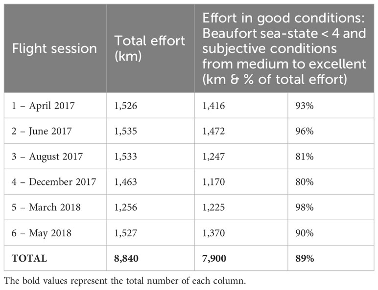
Table 3 Total effort and effort carried out with optimal observation conditions (in km) per flight session.
Sightings recorded during the six flight sessions, detailed in Appendix E, included 1,120 sightings of harbour porpoises (1,412 individuals) and 4,344 seabird sightings (5,861 individuals). The seabird sightings included 1,218 sightings of auks, 1,385 of black-legged kittiwakes, 134 of cormorants, 186 of northern fulmars and 1,421 of northern gannets. These sightings included both individuals and groups.
For each species, the model with the lowest WAIC was selected (all models are tanked in Appendix F). These models were used to predict species distributions. All species except for cormorants were predicted to be distributed offshore. The predicted distribution of cormorants was very coastal. Four seasonal patterns of abundance could be defined post-hoc: some species were abundant in spring (March to May) and almost absent in summer (June to August); others were abundant in winter (December to February), species whose abundance varies annually, and the rest showed little seasonal variations throughout the year.
Auks. The highest estimated densities of auks were associated with low chlorophyll a concentrations, large distances to the coast and colonies, low sea surface temperatures and average current speeds (Figure 2). Auks were predicted in offshore areas except in the north-west of the study area (near the English coast) and near the Belgian coast where they were almost absent (Figure 3A). They were most abundant between October and May (density > 1 individual/km²) and almost absent in summer (density < 0.1 individuals/km², Appendix G) with about 120,800 individuals estimated in March [80% Credible Interval: CI (14,000 - 260,000)] and only 100 individuals estimated in August [CI (8 - 250); Appendix H]. The lowest uncertainties associated with the predictions and counterfactuals were obtained during the months when aerial surveys were conducted (Appendix I). Uncertainties were fairly homogeneous in the study area because it was homogeneously covered.
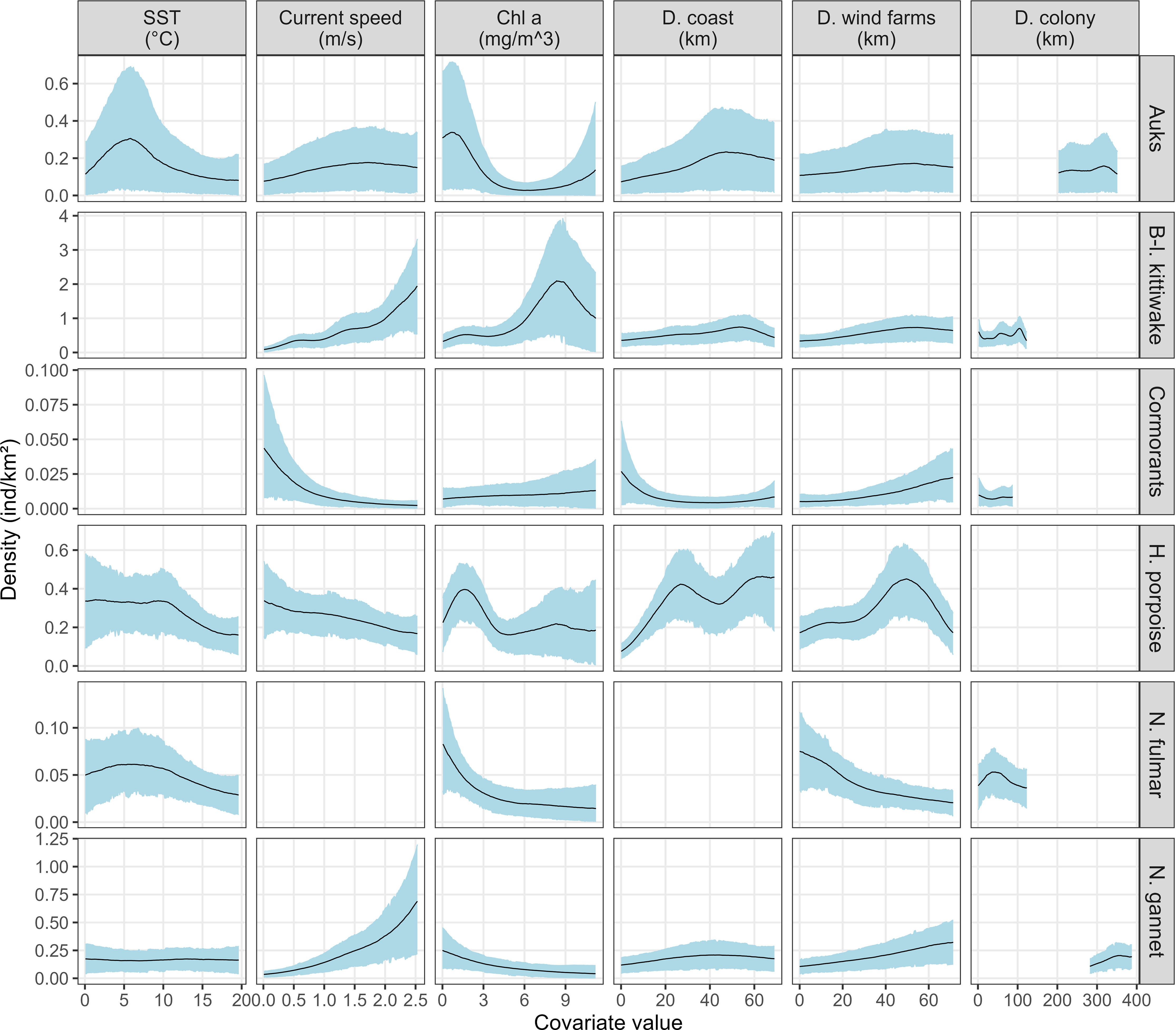
Figure 2 The average functional relationships between species and the selected variables. Solid lines represent the estimated smooth functions averaged over the entire period and the blue shaded regions show the approximate 95% confidence intervals (relationships obtained for each month are showed in Appendix F). The density of individuals is shown on the y-axis, where a zero indicates no effect of the covariate. A blank panel indicates that the variable was not selected in the model for this species group. SST: sea surface temperature, Chl a, chlorophyll a concentration; D. coast, distance to the coast; D. wind farms, distance to operational wind farms; D. colony, distance to the closest colony; B-l, black-legged; H, harbour; N, northern.
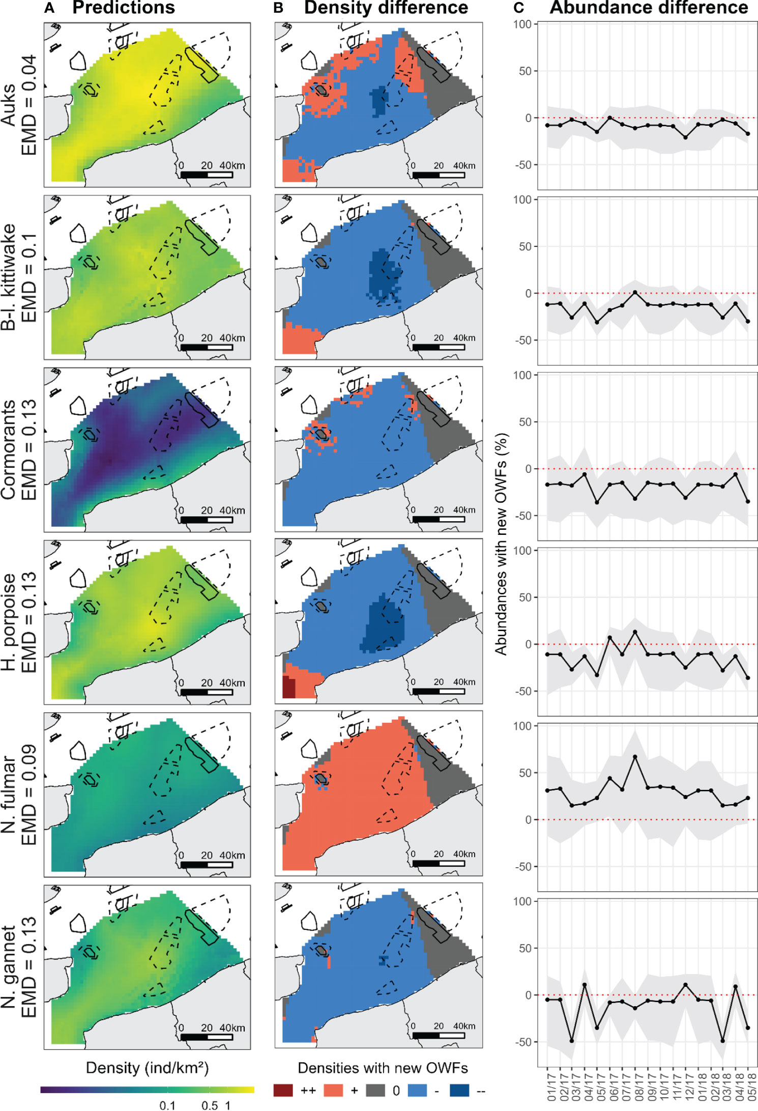
Figure 3 (A) The average predicted densities obtained from the models in the southern North Sea. Densities are averaged over the entire period. Monthly densities are shown in Appendix G Black solid boxes represent the wind farms in operation and black dashed boxes the wind farms in development. (B) The differences between counterfactuals and predicted densities. Reds and oranges indicate that densities increased when the new OWFs were added; greys indicate that densities were not changed and blues indicate that densities decreased when the new OWFs were added. (C) The monthly differences between counterfactual and predicted abundance estimates (number of individuals). The differences are given from January 2017 to May 2018. Positive values indicate that abundances increased when the new OWFs were added while negative values indicate that abundances decreased. Grey shaded regions represent confidence intervals.
Northern fulmars. The highest estimated densities of fulmars were associated with low chlorophyll a concentrations, low sea surface temperatures and short distances to colonies (Figure 2). Fulmars were distributed with high densities following a south-west/north-east axis that passed through the Dover Strait, especially in spring (March-April; Appendix G). Overall, abundances were quite low, reaching a maximum of 3,100 individuals in March [CI (150 – 8,650)] and a minimum of 280 [CI (10 - 570); Appendix H] in August. Uncertainties were quite high in all months (Appendix I) and particularly high in January and February, when no survey was conducted.
Black-legged kittiwakes. The highest estimated densities of black-legged kittiwakes were associated with high chlorophyll a concentrations, high current speeds and large distances to the coast (Figure 2). Kittiwakes were predicted to occur in the whole study area (Figure 3A) with an east-west shift in their distribution pattern over the year. The lowest abundance was estimated in August [≈ 4,700 individuals, CI (380 - 8,800)] and the highest in November [≈ 23,000 individuals; CI (750 - 65,600); Appendix H]. As for harbour porpoise, the lowest uncertainties were obtained during the months when aerial surveys were conducted (Appendix I). They were the highest in the centre of the study area.
Harbour porpoise. The highest estimated densities of harbour porpoises were associated with low chlorophyll a concentrations, distances to the coast of around 25-30 km and beyond 50 km, low current speed and low sea surface temperatures (Figure 2). As a result, harbour porpoises were not predicted in coastal areas but in offshore waters, with higher densities estimated further from the coasts (> 20 km, Figure 3A). Distribution patterns were relatively constant throughout the year but not the estimated densities and abundances. Estimated densities were the lowest in summer (maximum density ≈ 0.1 individuals/km²) and the highest in spring between March and May (maximum density ≈ 3-5 individuals/km²; Appendix G), with 2,500 individuals [CI (970 - 4,200)] estimated in summer (August) and up to 26,600 individuals [CI (5,700 - 52,200)] estimated in spring (May, Appendix H). A smaller peak of abundance to 16,400 individuals [CI (5,700 - 25,400)] was estimated in December. The lowest uncertainties associated with the predictions and counterfactuals were obtained during the months when aerial surveys were conducted (Appendix I). They were the highest in the centre of the study area.
Cormorants. The highest estimated densities of cormorants were close to the colonies in shallow waters associated with low current speeds (Figure 2). Their resulting distribution was very coastal, predicted to be mainly along the French and Belgian coasts (Figure 3A) with little variation throughout the year. They were most abundant in March [≈ 2,700 individuals, CI (10 – 9,000), Appendix H]. Uncertainties were high for cormorants, particularly when no survey was conducted and offshore when surveys were conducted (Appendix I).
Northern gannets. The highest estimated densities of northern gannets were associated with high current speeds, low chlorophyll a concentrations and large distances to the coast and colonies (Figure 2). Gannets were mostly predicted to occur in the centre of the study area (Figure 3A). They were more abundant in December and March with up to 10,000 individuals [CI (950 – 35,000)] and down to 3,000 - 4,000 individuals during the other months (Appendix H). Uncertainties were high when no survey was conducted and offshore when surveys were conducted and were fairly homogenous (Appendix I).
The relationships between predicted densities and distance to operational OWFs varied between species groups (Figure 2). Predicted densities of northern fulmars were higher at short distances to OWFs while densities of auks were insensitive to distance to OWFs. In contrast, the highest densities of kittiwakes, cormorants, porpoises and gannets were found at distances larger than 40 km from OWFs.
The estimated distribution of all species in the eastern and north-western part of the study area remained unchanged when predictions from the prospective scenario, wherein all planned OWFs were assumed to be operating, were taken into account (Figure 3B). For porpoises, kittiwakes, gannets and cormorants, densities would be lower, on average, in the centre of the study area, particularly near the planned OWFs. Densities of fulmars would however be higher in this central area. The predicted change in auk distribution was more contrasted: densities were predicted to be lower in the centre of the study area but higher in the northern and western parts.
The EMDs, which indicated the match between the predicted density distributions and the counterfactual density distributions, were relatively small (less than 0.3; Figure 4). Therefore, the counterfactual predictions were relatively close to the original predictions, but the values were not negligible, so the implementation of the OWFs would affect species distribution. This would be particularly noticeable in spring for harbour porpoise, black-legged kittiwake and northern gannet (higher EMDs), in summer for northern fulmar and throughout the year for cormorants. For auks, the EMDs were relatively stable, so the implementation of the OWFs would probably not have a major impact on the distribution of the species.
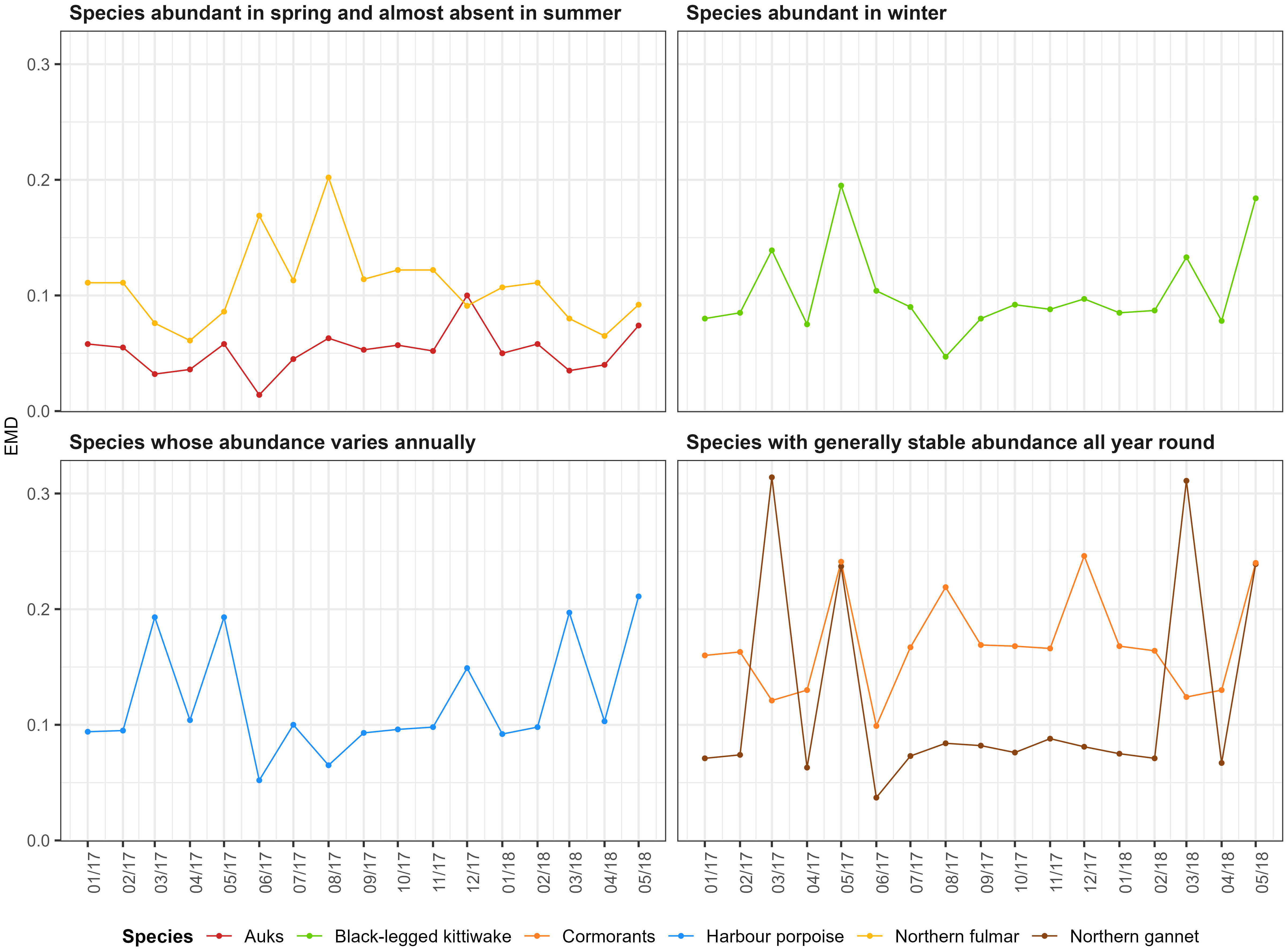
Figure 4 The earth mover’s distance (EMD) per species per month. The EMD is calculated as the distance between the model and counterfactual predictions. A value of 0 indicates a perfect match between the model and counterfactual predictions.
In contrast, if the planned OWFs were operational, the impact on species abundance would be higher. The abundance of fulmars would increase significantly (between +20% and +70%; Figure 3C), all else being equal, while the abundance of all other species would decrease (down to -50% for gannets), although the decrease would be less for auks (maximum -20%). There are two months during the time period where abundances of porpoises and gannets slightly increase (+10%; Figure 3C).
For the year 2017/2018, using an approximate BAG method, we highlighted high intra-annual variability in distribution patterns with species mostly present in spring, or in winter, or both in spring and winter, or all year round. To minimise the impacts of OWFs currently planned in the area, construction should consider that species are not equally distributed within a year, and consequently take place in areas and seasons during which animals are present in the lowest densities. Our results highlighted summer as the season where seabirds and harbour porpoises were present in the lowest densities in the area. We also highlighted a potential change in species distribution and abundance after the planned OWFs come into operation, suggesting potential long-term effects on marine megafauna that need to be considered in a marine spatial planning context.
We are aware that we sampled only a few months of the year and we cannot represent fixed monthly or seasonal distribution patterns for the studied species over multiple years. However, our model, which included month-varying relationships and time-varying spatial effects (modelled as random walk; see Appendix C) allowed to predict species distributions for each month, thereby illustrating intra-annual variation.
Recommendations for minimisation measures critically hinge on knowledge of seasonal abundance and spatial distribution patterns. Carrying out regular surveys every month is very costly, and impractical over large areas. Here, we capitalised on a series of six surveys carried out between 2017 and 2018 to collect data on marine megafauna. These data were then used to calibrate a model that took into account spatio-temporal variations explicitly. In order to study mobile species, monitoring over a broad area is required which in turn limit temporal replicates. With six surveys spread over a whole year, we highlighted intra-annual variations in the species distribution allowing to identify the period and areas where the impact would be the lowest while with an average annual distribution, we would not have been able to do it. This study therefore highlights how critical spatial and seasonal variations in abundance are to marine spatial planning.
The estimated relationships between animal distributions and the planned OWFs must be interpreted with caution: they are not causal, nor do they arise from direct observations of behavioural responses to OWFs. Instead they could reflect the effect of other variables (e.g. environmental) not considered in the models.
Our predictions are borne out of the best available evidence for the study area, and rely on a state-of-the-art modelling approach that takes into account seasonal and spatial variations. Regular monitoring of the study area in the future can ground-truth these predictions. Our prospective approach allows for the cumulative effect of the commissioning of multiple OWFs (either operating or planned) on marine megafauna distribution to be quantified, in contrast to the DEPONS model (Nabe-Nielsen et al., 2018), which assesses the cumulative impact of noise on harbour porpoise distribution during the construction phase of multiple OWFs. The approach and results we put forward in this study suggest additional impacts of OWFs than those determined using the DEPONS model. The DEPONS model considers the cumulative impact of noise from OWF projects built simultaneously or sequentially, while our approach targets various species, not only those impacted by noise, and assesses the long-term impacts on species distributions once planned OWFs are operational, and not only the impacts during the construction phase. These two approaches complement one another and are both crucial to mitigation efforts and marine spatial planning objectives with regards to the impacts of OWFs at the population scale since they individually concern the construction and operational phases.
Harbour porpoises showed an offshore distribution and were absent along the coast line, as previously highlighted by Lambert et al. (2017). They appeared to prefer cool waters, which may explain their decreased abundance in summer compared to winter and spring. It is likely that they migrate to the central and northern parts of the North Sea in summer (Benke et al., 2014; McClellan et al., 2014).
Most seabirds were predicted to be more abundant further offshore with monthly variations in their abundances with the exception of cormorants, which had a coastal distribution, which is consistent with Lambert et al. (2017) and Virgili et al. (2017). This is because non-breeding cormorants feed within a radius of 35 km around their colonies and resting sites (Grémillet, 1997). Auks and fulmars were mostly abundant in spring and winter and absent from the study area in summer. This is because auks start migrating to their wintering grounds between May and October (Heath et al., 2000; Fort et al., 2013) and fulmars between June and November (Cadiou et al., 2004; Lambert et al., 2017). Kittiwakes were abundant in winter, which is when they are concentrated around breeding colonies, and less abundant in summer when they are dispersed far from colonies (Marchant et al., 2002). The highest abundances of northern gannets were estimated at the beginning of spring, the prenuptial period during which many individuals cross the Dover Strait (Fort et al., 2012). Individuals observed between April and September were probably immature birds because mature individuals breed outside of the study area (Kubetzki et al., 2009; Fort et al., 2012; Wakefield et al., 2013).
In this study, we applied the approach proposed by Methratta (2020), consisting in recording species sightings at different distances from wind farms and to include the distance to the wind farms in the models. We thus estimated relationships between the sightings and the distance to the nearest OWF as well as with variables that characterise the environment. The results were consistent with the known ecology of the species (Grémillet, 1997; Heath et al., 2000; Marchant et al., 2002; Cadiou et al., 2004; Fort et al., 2012; 2013; Benke et al., 2014; McClellan et al., 2014; Lambert et al., 2017). The transect design carried out during the surveys does not strictly follow the BAG design because it was not a sampling at increasing distances from the wind farms but rather a sampling that allowed the area to be optimally gridded with an aircraft (limitation of transit time with optimal coverage). We have therefore adapted the approach proposed by Methratta (2020) to the aerial survey methodology. We highlighted the effect of the OWF present in the area and use the obtained relationships to predict the distribution that species would have if these relationships were maintained with the OWFs currently planned in the area.
The models predicted the highest densities of fulmars at short distances to operational OWFs, whereas for all other groups, except auks, the highest densities were at large distances. Predicted densities of auks were unaffected by the distance to OWFs. Furness et al. (2013) and Vanermen et al. (2015) showed that gannets are sensitive to the presence of OWFs and would avoid them. This is supported in our results by the predictions of lower gannet densities near the operating OWFs in the area. Likewise, Vallejo et al. (2017) showed a constant abundance of common guillemot (an auk species) regardless of the development phases of an OWF, which may explain why the implementation of the planned OWFs had little effect on the auk abundance. Garthe and Hüppop (2004) have argued that cormorants, kittiwakes and fulmars were among the least sensitive species to the presence of OWFs. The model predicted higher densities of fulmars near OWFs, so if the planned OWFs were operational, their density in the study area would increase, all else being equal. Harbour porpoises seem to avoid an OWF area during the construction phase but can become as abundant during the operational phase as before construction started (Madsen et al., 2006; Brandt et al., 2011; Vallejo et al., 2017). Here, densities of harbour porpoises were lower in the east, near the Belgian wind farm, than in the centre of the study area, this may be due to the construction of an extension around a Belgian OWF during the surveys.
The prediction of seabird and harbour porpoise distributions based on the hypothetical scenario in which all planned OWFs were fully operational highlighted changes in species distribution. These predictions can be compared to future monitoring data, putting the model’s predictive ability to a true test and ultimately facilitating the improvement of predictive models. Northern fulmar abundance was predicted to increase near the new OWFs while the abundance of the other groups decreased, suggesting avoidance of OWFs and thus displacement of individuals out of the study area. One hypothesis for the unexpected increase in fulmar abundance, proposed for example by Vanermen et al. (2015), would be that feeding opportunities would be enhanced near OWFs, but any attraction effects of OWFs are currently poorly understood. These predicted changes in abundance and distribution clearly suggest that new OWFs in the study area would impact marine megafauna when construction is finalised and they become operational.
The construction phase of an OWF poses the greatest threat to cetaceans because the noise generated by pile driving drives away the animals (Vallejo et al., 2017) and can induce hearing loss (Tougaard et al., 2004; Thomsen et al., 2006; Dähne et al., 2013). During the operational phase, the noise levels generated by the turbines and maintenance activities are lower than those during pile driving and are unlikely to affect cetaceans (Madsen et al., 2006). The operational phase is the most hazardous for seabirds because of fatal collisions with wind turbines, particularly for gannets (Furness et al., 2013) but also because turbines may create physical barriers along migration routes and displace animals from foraging habitats (Drewitt and Langston, 2006; Furness et al., 2013). Displacement occurs when seabirds avoid OWFs and can lead to increased energy costs and reduced food supplies which might affect individual fitness (Masden et al., 2010; Peschko et al., 2020).
In order to meet the mitigation objectives of avoidance and minimisation (Kiesecker et al., 2010), based on our results, we recommend that wind farms be established in areas of low seabird densities to minimise the risk of collisions and the loss of important foraging habitats during the operational phase, and that the construction phase be planned during periods of low porpoise densities. We would mainly recommend that the various OWFs planned for development be constructed between mid-summer and early fall to minimise the impact on harbour porpoises. The construction phase of a wind farm takes between 1.5 and 2 years, depending, in part, on the number of wind turbines constructed (Carstensen et al., 2006). Some stages of the construction phase are noisier than others and last between 3 and 5 months (Carstensen et al., 2006; Brandt et al., 2011). Therefore, the time window proposed in the study would be compatible with the most noise-generating construction stages of the wind farms. In addition, weather conditions in the area are generally most favourable between mid-summer and fall, which could facilitate the construction phase and limit its duration.
Another recommendation could be to avoid building OWFs in offshore areas in the centre of the study area to minimise the impact on seabirds, in particular auks, kittiwakes and gannets. In the light of these recommendations, the two wind farms planned off the Belgian coast (between 2.5 and 2.8° E and 51.25 and 51.7° N; Figure 1) could be harmful to seabirds because the southern North Sea is a migration corridor for numerous seabirds (Stienen et al., 2007). In order to apply this recommendation, further research would probably be required, particularly into the distribution of the species’ prey and whether the construction of the OWFs would result in the displacement of this prey, in which case the loss of habitat would probably be limited. In addition, the main impact of the OWFs would be collisions with seabirds. A better understanding of seabird behaviour in the presence of OWFs, particularly through telemetry, would help to fill in the gaps.
To minimise this impact, we also recommend that the number of OWFs constructed in the coming years be limited, and that the new OWFs be spaced more widely apart, avoiding high concentrations of farms in a small area. The construction of OWFs in various areas should also be staggered temporally so that the disruption occurs only in a limited area at a time, allowing animals, especially cetaceans, areas of refuge in which they can continue foraging, breeding, etc. undisturbed. It is essential that the location of OWFs avoids bird migration corridors (Larsen and Madsen, 2000; Garthe and Hüppop, 2004), and the layout of the turbines must avoid the barrier effect if the wind farm is located on a migration corridor. Turbines could be controlled to limit their operation during periods of high bird migration (Fijn et al., 2015). Finally, the definition, at national or even European level, of zones that are favourable or unfavourable for the installation of wind turbines would allow better positioning of wind farms while limiting the impact on biodiversity.
This study predicts the potential impact of wind farms on marine megafauna species, but in a wider context, marine species are subject to anthropogenic pressures beyond those resulting from OWFs, and in the North Sea those pressures are many. The southern North Sea is crossed by a shipping lane frequently used by more than 400 commercial ships (1/4 of the world traffic), many ferries as well as fishing and recreational vessels, which certainly have an impact on marine megafauna (Halpern et al., 2008). For example, Wisniewska and colleagues (Wisniewska et al., 2018) showed that porpoises make deeper dives and interrupt their foraging and echolocation activities due to the noise of boats. Fishing also affects seabird and cetacean populations through the alteration of food supplies and bycatch incidents in fishing gear (Tasker et al., 2000; Read et al., 2006). The cumulative impacts of boat noise, fishing and wind farm activities could have negative long-term consequences on marine megafauna. These impacts are important to consider in the context of marine spatial planning in order to establish and maintain an organised maritime area that takes the interactions between users (both professional and private) into account and balances the need for maritime development and activities with the protection of the environment (Douvere, 2008; European Parliament and Council Directive 2014/89/EU). The better we understand the impacts of anthropogenic activities – individually and cumulatively, on a specific and broad scale – the more effectively we can reconcile development and environmental conservation and make valuable suggestions for marine spatial planning.
The southern North Sea is subjected to intense human activities that include high maritime traffic (commercial, fishing and tourist vessels) as well as a high concentration of OWFs. The region is also densely populated by seabirds and harbour porpoises. It is crucial that we understand how marine megafauna use their environment and how they respond to maritime activities in order to 1) anticipate the effects of anthropogenic pressures, both current and future, on the animals that inhabit this region and 2) to make a guided effort to mitigate them. With mobile species, it is important to define how their distribution and abundance may change over time. Our study illustrates how the regular monitoring of marine megafauna in a relatively small area over several seasons enables the prediction of monthly distributions and abundances and changes thereof under hypothetical scenarios of increased human activities. Our study also illustrates how the BAG design can be used on aerial survey data. In addition to being promising for fisheries surveys, the BAG design approach has shown promising results in assessing the impact of wind farms on large predators such as cetaceans and seabirds.
One of the objectives of the European Union Member States is to contribute to the sustainable development of energy sectors at sea, maritime transport, and the fisheries and aquaculture sectors, but their role also includes ensuring the preservation and protection of the environment. This study aims to inform marine spatial planning decisions regarding these developments so that they have the least possible impact on marine species. Our goal was to reconcile the development of wind farm activity with the conservation of marine megafauna species by anticipating the potential impacts the existing and planned developments would have on various species using the best available evidence. While a prospective assessment helps in planning and decision making, it remains paramount to ensure that regular and accurate monitoring of the study area continues in order to ground-truth predictions and revise models accordingly both for future marine spatial planning and mitigation purposes.
The datasets presented in this study can be found in online repositories. The names of the repository/repositories and accession number(s) can be found below: https://pelabox.univ-lr.fr/pelagis/PelaObs/.
Ethical approval was not required for the study involving animals in accordance with the local legislation and institutional requirements because the research methods were purely observational.
AV: Conceptualization, Formal analysis, Methodology, Writing – original draft. SL: Data curation, Writing – review & editing. MA: Conceptualization, Formal analysis, Writing – review & editing. GD: Data curation, Writing – review & editing. OC: Data curation, Writing – review & editing. JS: Supervision, Writing – review & editing.
The author(s) declare financial support was received for the research, authorship, and/or publication of this article. This study was funded by the national project LEDKOA (Levée des risques pour l’appel d’offres éolien au large de Dunkerque par observation aérienne) survey (Agence Francise pour la Biodiversité 2016/129). Pelagis was supported by the French ministry in charge of Environment (Direction de l’Eau et de la Biodiversité).
We thank above all the Direction Générale de l’Energie et du Climat, the Office Français de la Biodiversité (formerly the Agence Française pour la Biodiversité) and the CEREMA that enabled us to carry out this study and Sylvain Michel who coordinated the project. Surveys would not have been possible without the investment and flexibility of the Pixair Survey team that conducted the flight sessions: Jean-Jérôme Houdaille, Pierre Chevé and Christian Morales; and the team of observers: Cécile Dars (Pelagis), Ghislain Dorémus (Pelagis), Marc Duvilla (LPO Normandie), Sophie Laran (Pelagis), Morgane Perri (Al Lark) and Olivier Van Canneyt (Pelagis). We would also like to thank the air traffic control agencies that facilitated the access to the study area: the DGAC and the Air Navigation Service (SNA NORD) for France; BELGOCONTROL and the Koksijde Control Tower for Belgium; the Luchtverkeersleiding Nederland for the Netherlands; and NATS for England. We thank Carin Reisinger for proofreading the manuscript and contributing to its improvement. Finally, we would like to thank the two reviewers for their careful reading and constructive comments, which allowed us to improve the manuscript.
The authors declare that the research was conducted in the absence of any commercial or financial relationships that could be construed as a potential conflict of interest.
All claims expressed in this article are solely those of the authors and do not necessarily represent those of their affiliated organizations, or those of the publisher, the editors and the reviewers. Any product that may be evaluated in this article, or claim that may be made by its manufacturer, is not guaranteed or endorsed by the publisher.
The Supplementary Material for this article can be found online at: https://www.frontiersin.org/articles/10.3389/fmars.2024.1344013/full#supplementary-material
Appendix A | Effort carried out during each flight session.
Appendix B | Colonies of seabirds located near the study area.
Appendix C | Details about the model used in the study.
Appendix D | Average monthly distributions of environmental variables used in the density surface modelling.
Appendix E | Sightings recorded during each flight session.
Appendix F | Models results.
Appendix G | Monthly predicted densities in the southern North Sea.
Appendix H | Monthly abundances in number of individuals estimated from the model (A) and the counterfactuals (B).
Appendix I | Coefficients of variation associated with the prediction and the counterfactuals.
Benke H., Bräger S., Dähne M., Gallus A., Hansen S., Honnef C. G., et al. (2014). Baltic Sea harbour porpoise populations: status and conservation needs derived from recent survey results. Mar. Ecol. Prog. Ser. 495, 275–290. doi: 10.3354/meps10538
Bergström L., Kautsky L., Malm T., Rosenberg R., Wahlberg M., Capetillo N.Å., et al. (2014). Effects of offshore wind farms on marine wildlife - a generalized impact assessment. Environ. Res. Lett. 9, 34012. doi: 10.1088/1748-9326/9/3/034012
Bergström L., Sundqvist F., Bergström U. (2013). Effects of an offshore wind farm on temporal and spatial patterns in the demersal fish community. Mar. Ecol. Prog. Ser. 485, 199–210. doi: 10.3354/meps10344
Board and National Research Council. (2005). Marine mammal populations and ocean noise: determining when noise causes biologically significant effects (Washington, DC: National Academies Press).
Brandt M. J., Diederichs A., Betke K., Nehls G. (2011). Responses of harbour porpoises to pile driving at the Horns Rev II offshore wind farm in the Danish North Sea. Mar. Ecol. Prog. Ser. 421, 205–216. doi: 10.3354/meps08888
Buckland S. T., Anderson D. R., Burnham H. P., Laake J. L., Borchers D. L., Thomas L. (2001). Introduction to distance sampling: Estimating abundance of biological populations (Oxford: Oxford University Press). doi: 10.1093/oso/9780198506492.001.0001.
Cadiou B., Pons J.-M., Yésou P. (2004). Oiseaux marins nicheurs de France métropolitaine: 1960–2000 (Mèze, Hérault: Biotope Editions).
Carstensen J., Henriksen O. D., Teilmann J. (2006). Impacts of offshore wind farm construction on harbour porpoises: acoustic monitoring of echolocation activity using porpoise detectors (T-PODs). Mar. Ecol. Prog. Ser. 321, 295–308. doi: 10.3354/meps321295
Dähne M., Gilles A., Lucke K., Peschko V., Adler S., Krügel K., et al. (2013). Effects of pile-driving on harbour porpoises (Phocoena phocoena) at the first offshore wind farm in Germany. Environ. Res. Lett. 8, 25002. doi: 10.1088/1748-9326/8/2/025002
Degraer S., Brabant R., Rumes B., Vigin L. (2018). Environmental Impacts of Offshore Wind Farms in the Belgian Part of the North Sea: Assessing and Managing Effect Spheres of Influence. (Brussels: Royal Belgian Institute of Natural Sciences, OD Natural Environment, Marine Ecology and Management). 136 p.
Dormann C. F., Elith J., Bacher S., Buchmann C., Carl G., Carré G., et al. (2013). Collinearity: a review of methods to deal with it and a simulation study evaluating their performance. Ecography 36, 27–46. doi: 10.1111/j.1600-0587.2012.07348.x
Douvere F. (2008). The importance of marine spatial planning in advancing ecosystem-based sea use management. Mar. Policy 32, 762–771. doi: 10.1016/j.marpol.2008.03.021
Drewitt A. L., Langston R. H. (2006). Assessing the impacts of wind farms on birds. Ibis 148, 29–42. doi: 10.1111/j.1474-919X.2006.00516.x
ESRI (2016). ArcGIS - A Complete Integrated System Environmental Systems (Redlands, California: Research Institute, Inc.). Available at: http://esri.com/arcgis.
European Commission (2023) European Wind Power Action Plan. COM(2023) 669 final. Available online at: https://eur-lex.europa.eu/legal-content/EN/TXT/PDF/?uri=CELEX:52023DC0669.
European Parliament and Council Directive 2014/89/EU European Parliament and Council Directive 2014/89/EU of 23 July 2014 establishing a framework for maritime spatial planning. Available at: https://eur-lex.europa.eu/legal-content/EN-FR/TXT/?uri=CELEX:32014L0089&from=FR.
Fijn R. C., Krijgsveld K. L., Poot M. J., Dirksen S. (2015). Bird movements at rotor heights measured continuously with vertical radar at a Dutch offshore wind farm. Ibis 157, 558–566. doi: 10.1111/ibi.12259
Foley M. M., Halpern B. S., Micheli F., Armsby M. H., Caldwell M. R., Crain C. M., et al. (2010). Guiding ecological principles for marine spatial planning. Mar. Policy 34, 955–966. doi: 10.1016/j.marpol.2010.02.001
Fort J., Pettex E., Tremblay Y., Lorentsen S. H., Garthe S., Votier S., et al. (2012). Meta-population evidence of oriented chain migration in northern gannets (Morus bassanus). Front. Ecol. Environ. 10, 237–242. doi: 10.1890/110194
Fort J., Steen H., Strøm H., Tremblay Y., Grønningsæter E., Pettex E., et al. (2013). Energetic consequences of contrasting winter migratory strategies in a sympatric Arctic seabird duet. J. Avian Biol. 44, 255–262. doi: 10.1111/j.1600-048X.2012.00128.x
Furness R. W., Wade H. M., Masden E. A. (2013). Assessing vulnerability of marine bird populations to offshore wind farms. J. Environ. Manage. 119, 56–66. doi: 10.1016/j.jenvman.2013.01.025
Garthe S., Hüppop O. (2004). Scaling possible adverse effects of marine wind farms on seabirds: developing and applying a vulnerability index. J. Appl. Ecol. 41, 724–734. doi: 10.1111/j.0021-8901.2004.00918.x
Gilles A., Adler S., Kaschner K., Scheidat M., Siebert U. (2011). Modelling harbour porpoise seasonal density as a function of the German Bight environment: implications for management. Endangered species Res. 14, 157–169. doi: 10.3354/esr00344
Gilles A., Viquerat S., Becker E. A., Forney K. A., Geelhoed S. C. V., Haelters J., et al. (2016). Seasonal habitat-based density models for a marine top predator, the harbour porpoise, in a dynamic environment. Ecosphere 7, 1–22. doi: 10.1002/ecs2.1367
Green R. H. (1979). Sampling Design and Statistical Methods for Environmental Biologists (New York, NY: John Wiley and Sons).
Grémillet D. (1997). Catch per unit effort, foraging efficiency, and parental investment in breeding great cormorants (Phalacrocorax carbo). ICES J. Mar. Sci. 54, 635–644. doi: 10.1006/jmsc.1997.0250
Guisan A., Thuiller W. (2005). Predicting species distribution: offering more than simple habitat models. Ecol. Lett. 8, 993–1009. doi: 10.1111/j.1461-0248.2005.00792.x
Halpern B. S., Walbridge S., Selkoe K. A., Kappel C. V., Micheli F., D’agrosa C., et al. (2008). A global map of human impact on marine ecosystems. Science 319, 948–952. doi: 10.1126/science.1149345
Hastie T., Tibshirani R. (1986). Generalized additive models. Stat. Sci. 3, 297–313. doi: 10.1214/ss/1177013604.
Heath M. F., Borggreve C., Peet N. (2000). European bird populations : estimates and trends (Cambridge: BirdLife International), 10.
Isaac N. J., Jarzyna M. A., Keil P., Dambly L. I., Boersch-Supan P. H., Browning E., et al. (2019). Data integration for large-scale models of species distributions. Trends Ecol. Evol. 35 (1), 56–67. doi: 10.1016/j.tree.2019.08.006
Kiesecker J. M., Copeland H., Pocewicz A., McKenney B. (2010). Development by design: blending landscape-level planning with the mitigation hierarchy. Front. Ecol. Environ. 8, 261–266. doi: 10.1890/090005
King S. L., Schick R. S., Donovan C., Booth C. G., Burgman M., Thomas L., et al. (2015). An interim framework for assessing the population consequences of disturbance. Methods Ecol. Evol. 6 (10), 1150–1158. doi: 10.1111/2041-210X.12411
Kranstauber B., Smolla M., Safi K. (2017). Similarity in spatial utilization distributions measured by the earth mover’s distance. Methods Ecol. Evol. 8, 155–160. doi: 10.1111/2041-210X.12649
Kranstauber B., Smolla M., Scharf A. K. (2018) move: Visualizing and Analyzing Animal Track Data. R package version 3.1.0. Available online at: https://CRAN.R-project.org/package=move.
Kubetzki U., Garthe S., Fifield D., Mendel B., Furness R. W. (2009). Individual migratory schedules and wintering areas of northern gannets. Mar. Ecol. Prog. Ser. 391, 257–265. doi: 10.3354/meps08254
Lambert C., Authier M., Doremus G., Gilles A., Hammond P., Laran S., et al. (2019). The effect of a multi-target protocol on cetacean detection and abundance estimation in aerial surveys. R. Soc. Open Sci. 6, 190296. doi: 10.1098/rsos.190296
Lambert C., Pettex E., Dorémus G., Laran S., Stéphan E., Van Canneyt O., et al. (2017). How does ocean seasonality drive habitat preferences of highly mobile top predators? Part II: The eastern North-Atlantic. Deep Sea Res. Part II: Topical Stud. Oceanogr. 141, 133–154. doi: 10.1016/j.dsr2.2016.06.011
Larsen J. K., Madsen J. (2000). Effects of wind turbines and other physical elements on field utilization by pink-footed geese (Anser brachyrhynchus): A landscape perspective. Landscape Ecol. 15, 755–764. doi: 10.1023/A:1008127702944
Legroux N., Ponchon A., Poirson C., Michel S. (2017). Synthèse bibliographique sur les oiseaux migrateurs, nicheurs et hivernants dans le détroit du Pas-de-Calais. 173. Available at: https://www.eoliennesenmer.fr/sites/eoliennesenmer/files/fichiers/2021/08/1_Avifaune-Etat-initial.pdf.
Madsen P. T., Wahlberg M., Tougaard J., Lucke K., Tyack P. (2006). Wind turbine underwater noise and marine mammals: implications of current knowledge and data needs. Mar. Ecol. Prog. Ser. 309, 279–295. doi: 10.3354/meps309279
Marchant J., Wernham C., Toms M., Baillie S., Siriwardena G., Clark J. (2002). The migration atlas: movements of the birds of Britain and Ireland. London: T. & A. D. Poyser.
Marques A. T., Batalha H., Bernardino J. (2021). Bird displacement by wind turbines: assessing current knowledge and recommendations for future studies. Birds 2, 460–475. doi: 10.3390/birds2040034
Masden E. A., Haydon D. T., Fox A. D., Furness R. W. (2010). Barriers to movement: modelling energetic costs of avoiding marine wind farms amongst breeding seabirds. Mar. pollut. Bull. 60, 1085–1091. doi: 10.1016/j.marpolbul.2010.01.016
McClellan C. M., Brereton T., Dell’Amico F., Johns D. G., Cucknell A. C., Patrick S. C., et al. (2014). Understanding the distribution of marine megafauna in the English Channel region: identifying key habitats for conservation within the busiest seaway on earth. PloS One 9, e89720. doi: 10.1371/journal.pone.0089720
Mendel B., Schwemmer P., Peschko V., Müller S., Schwemmer H., Mercker M., et al. (2019). Operational offshore wind farms and associated ship traffic cause profound changes in distribution patterns of Loons (Gavia spp.). J. Environ. Manage. 231, 429–438. doi: 10.1016/j.jenvman.2018.10.053
Methratta E. T. (2020). Monitoring fisheries resources at offshore wind farms: BACI vs. BAG designs. ICES J. Mar. Sci. 77, 890–900. doi: 10.1093/icesjms/fsaa026
Miller D. L., Burt M. L., Rexstad E. A., Thomas L. (2013). Spatial models for distance sampling data: recent developments and future directions. Methods Ecol. Evol. 4, 1001–1010. doi: 10.1111/2041-210X.12105
Nabe-Nielsen J., van Beest F. M., Grimm V., Sibly R. M., Teilmann J., Thompson P. M. (2018). Predicting the impacts of anthropogenic disturbances on marine populations. Conserv. Lett. 11, e12563. doi: 10.1111/conl.12563
Peschko V., Mendel B., Müller S., Markones N., Mercker M., Garthe S. (2020). Effects of offshore windfarms on seabird abundance: Strong effects in spring and in the breeding season. Mar. Environ. Res. 162, 105157. doi: 10.1016/j.marenvres.2020.105157
Pitchford J. L., Howard V. A., Shelley J. K., Serafin B. J., Coleman A. T., Solangi M. (2016). Predictive spatial modelling of seasonal bottlenose dolphin (Tursiops truncatus) distributions in the Mississippi Sound. Aquat. Conserv.: Mar. Freshw. Ecosyst. 26, 289–306. doi: 10.1002/aqc.2547
Read A. J., Drinker P., Northridge S. P. (2006). Bycatch of marine mammals in U.S. and global fisheries. Conserv. Biol. 20, 163–169. doi: 10.1111/j.1523-1739.2006.00338.x
Roberts J. J., Best B. D., Dunn D. C., Treml E. A., Halpin P. N. (2010). Marine Geospatial Ecology Tools: An integrated framework for ecological geoprocessing with ArcGIS, Python, R, MATLAB, and C++. Environ. Model. Softw. 25, 1197–1207. doi: 10.1016/j.envsoft.2010.03.029
SAMMOA 1.0.4 Système d’Acquisition des données sur la Mégafaune Marine par Observations Aériennes, logiciel développé par l’UMS 3462 Pelagis et Code Lutin. Available online at: http://www.observatoire-pelagis.cnrs.fr/publications/les-outils/article/logiciel-sammoa.
Santos C. F., Agardy T., Andrade F., Crowder L. B., Ehler C. N., Orbach M. K. (2019). Major challenges in developing marine spatial planning. Mar. Policy. 132, 103248. doi: 10.1016/j.marpol.2018.08.032
Stienen E. W., Van Waeyenberge J., Kuijken E., Seys J. (2007). Trapped within the corridor of the Southern North Sea: the potential impact of offshore wind farms on seabirds. 1st ed (Madrid: Birds and wind farms. Risk assessment and mitigation), 71–80. Quercus.
Strindberg S., Buckland S. T. (2004). Zigzag survey designs in line transect sampling. Journal of Agricultural. Biol. Environ. Stat 9, 443. doi: 10.1198/108571104X15601
Tasker M. L., Camphuysen C. J., Cooper J., Garthe S., Montevecchi W. A., Blaber S. J. (2000). The impacts of fishing on marine birds. ICES J. Mar. Sci. 57, 531–547. doi: 10.1006/jmsc.2000.0714
Thomas L., Buckland S. T., Rexstad E. A., Laake J. L., Strindberg S., Hedley S. L., et al. (2010). Distance software: design and analysis of distance sampling surveys for estimating population size. J. Appl. Ecol. 47, 5–14. doi: 10.1111/j.1365-2664.2009.01737.x
Thomsen F., Lüdemann K., Kafemann R., Piper W. (2006). Effects of offshore wind farm noise on marine mammals and fish. Biola Hamburg Germany behalf COWRIE Ltd 62.
Tougaard J., Teilmann J., Rye Hansen J. (2004). Effects of the horns reef wind farm on harbour porpoises. Report number NEI-DK--4697. (Denmark), 23.
Vallejo G. C., Grellier K., Nelson E. J., McGregor R. M., Canning S. J., Caryl F. M., et al. (2017). Responses of two marine top predators to an offshore wind farm. Ecol. Evol. 7, 8698–8708. doi: 10.1002/ece3.3389
Vanermen N., Onkelinx T., Courtens W., Van De Walle M., Verstraete H., Stienen E. W. (2015). Seabird avoidance and attraction at an offshore wind farm in the Belgian part of the North Sea. Hydrobiologia 756, 51–61. doi: 10.1007/s10750-014-2088-x
Vehtari A., Gelman A., Gabry J. (2017). Practical Bayesian model evaluation using leave-one-out cross-validation and WAIC. Stat comput. 27, 1413–1432. doi: 10.1007/s11222-016-9696-4.
Virgili A., Lambert C., Pettex E., Dorémus G., Van Canneyt O., Ridoux V. (2017). Predicting seasonal variations in coastal seabird habitats in the English Channel and the Bay of Biscay. Deep Sea Res. Part II: Topical Stud. Oceanogr. 141, 212–223. doi: 10.1016/j.dsr2.2017.03.017
Wakefield E. D., Bodey T. W., Bearhop S., Blackburn J., Colhoun K., Davies R., et al. (2013). Space partitioning without territoriality in gannets. Science 341, 68–70. doi: 10.1126/science.1236077
Whitt A. D., Dudzinski K., Laliberté J. R. (2013). North Atlantic right whale distribution and seasonal occurrence in nearshore waters off New Jersey, USA, and implications for management. Endangered Species Res. 20, 59–69. doi: 10.3354/esr00486
Wikle C., Royle J. (2002). Spatial statistical modeling in biology (Mississauga, ON: EOLSS Publishers Co. Ltd).
Wilber D. H., Carey D. A., Griffin M. (2018). Flatfish habitat use near North America’s first offshore wind farm. J. Sea Res. 139, 24–32. doi: 10.1016/j.seares.2018.06.004
Wisniewska D. M., Johnson M., Teilmann J., Siebert U., Galatius A., Dietz R., et al. (2018). High rates of vessel noise disrupt foraging in wild harbour porpoises (Phocoena phocoena). Proc. R. Soc B 285, 20172314. doi: 10.1098/rspb.2017.2314
Keywords: BAG design, counterfactuals, distribution and abundance, prospective impact, species distribution models
Citation: Virgili A, Laran S, Authier M, Dorémus G, Van Canneyt O and Spitz J (2024) Prospective modelling of operational offshore wind farms on the distribution of marine megafauna in the southern North Sea. Front. Mar. Sci. 11:1344013. doi: 10.3389/fmars.2024.1344013
Received: 24 November 2023; Accepted: 01 February 2024;
Published: 20 February 2024.
Edited by:
Mark Jessopp, University College Cork, IrelandReviewed by:
Oriol Giralt Paradell, University College Cork, IrelandCopyright © 2024 Virgili, Laran, Authier, Dorémus, Van Canneyt and Spitz. This is an open-access article distributed under the terms of the Creative Commons Attribution License (CC BY). The use, distribution or reproduction in other forums is permitted, provided the original author(s) and the copyright owner(s) are credited and that the original publication in this journal is cited, in accordance with accepted academic practice. No use, distribution or reproduction is permitted which does not comply with these terms.
*Correspondence: Auriane Virgili, YXVyaWFuZUBzaGFyZXRoZW9jZWFuLmVhcnRo
Disclaimer: All claims expressed in this article are solely those of the authors and do not necessarily represent those of their affiliated organizations, or those of the publisher, the editors and the reviewers. Any product that may be evaluated in this article or claim that may be made by its manufacturer is not guaranteed or endorsed by the publisher.
Research integrity at Frontiers
Learn more about the work of our research integrity team to safeguard the quality of each article we publish.