Seasonal variability of Red Sea mixed layer depth: the influence of atmospheric buoyancy and momentum forcing

The seasonal and spatial evolution of the mixed layer (ML) in the Red Sea (RS) and the influence of atmospheric buoyancy and momentum forcing are analyzed for the 2001–2015 period using a high-resolution (1/100°, 50 vertical layers) ocean circulation model. The simulation reveals a strong spatiotemporal variability reflecting the complex patterns associated with the air–sea buoyancy flux and wind forcing, as well as the significant impact of the basin’s general and mesoscale circulation. During the spring and summer months, buoyancy forcing intensifies stratification, resulting in a generally shallow ML throughout the basin. Nevertheless, the results reveal local maxima associated with the influence of mesoscale circulation and regular wind induced mixing. Under the influence of surface buoyancy loss, the process of deepening of the ML commences in early September, reaching its maximum depth in January and February. The northern Gulf of Aqaba and the western parts of the northern RS, exhibit the deepest ML, with a gradual shoaling toward the south, primarily due to the surface advection of relatively fresh water that enters the basin from the Gulf of Aden. The mixed layer depth (MLD) variability is primarily driven by atmospheric buoyancy forcing, especially its heat flux component. Although evaporative fluxes dominate the annually averaged surface buoyancy forcing, they exhibit weak seasonal and spatial variability. Wind induced mixing exerts a significant impact on the MLD only locally, especially during summer. Of particular importance are strong winds channeled by topography, such as those in the vicinity of the Strait of Bab-Al-Mandeb and the straits connecting the two gulfs in the north, as well as lateral jets venting through mountain gaps, such as the Tokar Jet in the central RS. The analysis highlights the complex patterns of air-sea interactions, thermohaline circulation, and mesoscale activity, all of them strongly imprinted on the MLD distribution.

1 Introduction

The surface mixed layer (ML) is the outermost layer of the ocean directly influenced by the atmosphere. Its thickness can vary from a few to hundreds of meters. The ML is characterized by uniformity in temperature and salinity, extending to a depth which practically reflects the penetration of the atmospheric impact on ocean’s upper layer (Kara, 2003). Consequently, the mixed layer depth (MLD) is a pivotal climatic factor that directly shapes the air-sea interaction processes. Furthermore, MLD plays a critical role in biological processes as mixing with deeper water can enrich the euphotic zone with nutrients or transport phytoplankton to deeper layers restricting sufficient photosynthesis (Mann and Lazier, 1991; Denman and Gargett, 1995).

The development of the ML is primarily driven by vertical mixing, which is generated by both wind-induced turbulence, through the shearing effects of momentum forcing, and by the stabilizing or destabilizing effects of sea-surface buoyancy fluxes on the water column. Surface momentum and buoyancy (the sum of heat and fresh water fluxes) are the primary drivers of mixing in the near-surface layer and the formation of the oceanic ML (Cronin and Sprintall, 2008). Buoyancy gain by the sea increases the stability of the surface layer, constraining the deepening of the ML. Conversely, air–sea buoyancy loss disrupts stratification, causing instability and convective mixing (Alexander et al., 2000; Kantha and Clayson, 2002; Carton et al., 2008). The upper layer stratification and the ML distribution are also affected by general and mesoscale circulation advecting heat and salt (Alexander et al., 2000; Taylor and Ferrari, 2010). Moreover, mesoscale eddies tend to homogenize the upper layers by inducing lateral and vertical mixing (Cerovečki and Marshall, 2008; Gaube et al., 2018; Zhan et al., 2019) and by displacing isopycnals; in particular, cyclonic eddies tend to cause the isopycnals to dome upward, locally decreasing the MLD, whereas anticyclonic eddies tend to deepen the isopycnals, locally increasing the MLD (Dong et al., 2014; Gaube et al., 2018). The variability of the ML is particularly important for semi-enclosed basins where an increase of ML thickness can lead to deep water formation that feeds the basin’s overturning circulation and oxygenates the near-bottom layers. Additionally, MLD and convection processes largely govern the vertical redistribution of nutrient concentration, which is of paramount importance for oligotrophic seas (Carvalho et al., 2019).

Located between Africa and the Arabian Peninsula, the Red Sea (RS) is an elongated semi-enclosed basin that extends from 12.5°N to 30°N in the SE–NW direction, with an average width of 220 km. Although its maximum depth along the axial trench exceeds 3000 m, shallow and broad shelf platforms cover a large part of the basin, especially in the Southern RS (SRS) (Rasul et al., 2015). The also elongated Gulfs of Aqaba (GoAq) and Suez (GoS) are basin’s extensions at its northeast and northwest tips, respectively (Figure 1). The GoS is very shallow, with an average depth of 40 m, and a mean width of approximately 30 km and extends to the northwest for approximately 300 km connected to the RS via a wide shelf. In contrast, the depth of the GoAq exceeds 1,800 m (Neumann and McGill, 1961) and the gulf is connected to the RS through the narrow Straits of Tiran, with a sill depth of approximately 260 m. In the southern RS, the relatively shallow (maximum depth of 137 m) and narrow (18 km) Strait of Bab-Al-Mandeb (BAM), connects the RS to the Gulf of Aden (GoAd) and the Indian Ocean (Figure 1).

Figure 1

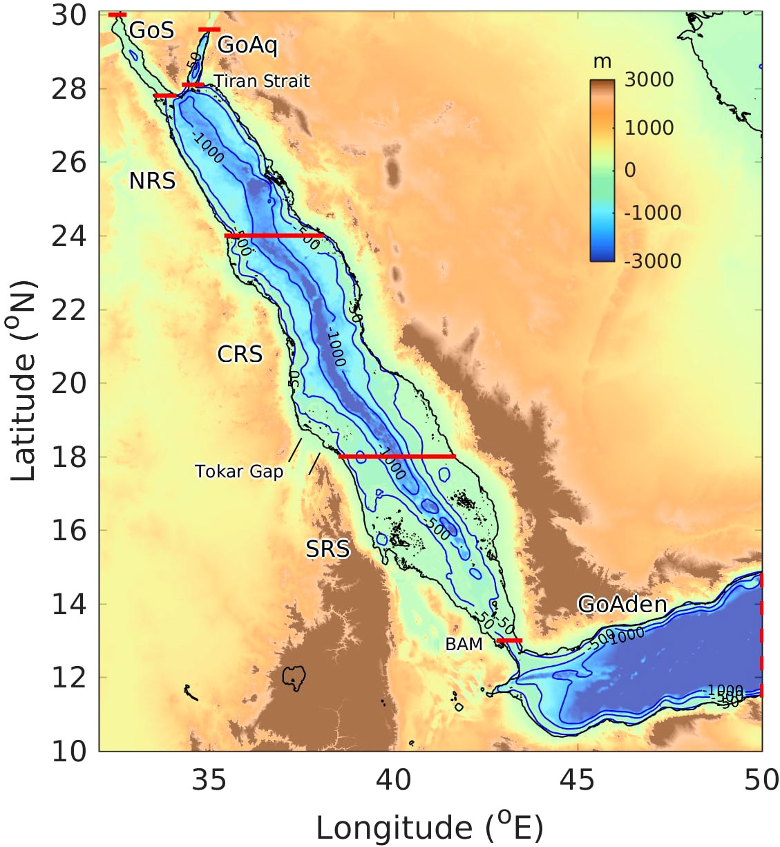
Figure 1 Bathymetric map of the model domain, covering the Red Sea (RS) and the adjacent gulfs. The red lines indicate the boundaries of the individual analysis regions: NRS, CRS, SRS, GoS, and GoAd. The dashed red line indicates the model’s open boundary.

Although the RS is located in the tropics, surrounded by two of the world’s largest deserts, it exhibits a weak annual net heat loss (7 W/m², Patzert, 1974; 11 ± 5 W/m², Sofianos et al., 2002). Because of its arid environment, the RS experiences one of the highest evaporation rates among the world’s oceans, with an annual average of approximately 2 m/year, while precipitation is negligible (Privett, 1959; Morcos, 1982; Tragou et al., 1999; Sofianos et al., 2002; Albarakati and Ahmad, 2013; Ahmad and Albarakati, 2015). The strongest air–sea buoyancy exchange occurs in winter in the northern RS, leading to convective mixing and the deepest mixed layers that guide the formation of two hypersaline water masses: the relatively lighter RS intermediate water (RSIW), which can be found below the surface water at a depth of up to about 250 m, and the denser RS deep water (RSDW) below it (Phillips, 1966; Cember, 1988; Sofianos and Johns, 2003; Yao et al., 2014a, b). These two water masses gradually flow southwards, with the RSIW accounting for most of the dense outflow through the BAM (see Figure 2 in Sofianos and Johns, 2015). The outflow of dense water from the RS through the BAM is counterbalanced by the inflow of fresher water from the GoAd (Sofianos and Johns, 2007). The exchange at the BAM exhibits a distinct seasonal pattern governed by the reversal of the monsoon winds and the associated upwelling in the GoAd (Patzert, 1974). In winter, the water exchange has a two-layered pattern in which the deep outflow is balanced by the inflow of surface water from the GoAd. In summer, the mean surface circulation reverses direction towards the GoAd, while fresher and cooler GoAd intermediate water (GAIW) intrude at intermediate depths (Yao et al., 2014a, b) and only a weak deep outflow persists throughout the summer (Yao et al., 2014a; Xie et al., 2019).

Figure 2

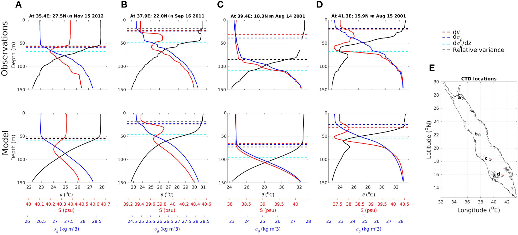
Figure 2 MLD estimates for selected profiles of salinity S, potential temperature θ, and potential density σ_θ, obtained using four methods: two property difference-based methods, with a σ_θ threshold of 0.125kg/m³ and a θ threshold that is equivalent to a σ_θ difference of 0.125kg/m³, the maximum gradient method based on σ_θ, and the relative variance method proposed by Huang et al. (2018) using σ_θ.

The importance of understanding the RS dynamical functioning has been increasingly recognized in recent years due to the basin’s ecological and economical significance, which stems from its remarkable biological diversity and productivity (Carvalho et al., 2019). Of particular importance for RS ecology is the wintertime surface heat loss in the NRS that drives the deepening of the mixed layer (ML) and the formation of the intermediate and deep waters that ventilate the deep parts of the RS. The deepening of the ML is a major factor driving the RS primary productivity (Acker et al., 2008; Gittings et al., 2018, 2019). The ML also plays a crucial role in the air–sea exchange of gases such as oxygen, thus impacting marine life (Gaube et al., 2018).

While observational studies have provided a general overview of the seasonal variability of the ML in the RS, knowledge about the MLD in the RS is still rather poor due to the paucity of in situ observations (Eladawy et al., 2017). The available observations are very inhomogeneous both in space and time; they have mostly been collected during periods of favorable sea conditions, thus providing a biased representation of the MLD distribution and hindering the identification of local extremes. Abdulla et al. (2018) derived the monthly MLD climatology in the RS based on a historical collection of temperature profiles from in situ observations between 1934 and 2017, suggesting large spatial and seasonal MLD variability. Particularly a deep ML has been observed in the NRS due to winter cooling of the highly saline surface water, while wind stress strongly affects MLD variability in the CRS and SRS (Abdulla et al., 2018). Ocean eddies and local wind jets, such as that at the Tokar Gap, significantly alter the MLD structure throughout the RS (Zhai and Bower, 2013; Abdulla et al., 2018; Krokos et al., 2021). In the GoAq, MLD variability is predominantly driven by variability in air–sea heat exchange (Wolf-Vecht et al., 1992; Silverman and Gildor, 2008; Carlson et al., 2014). Based on observations, Carlson et al. (2014) reported that the MLD in the GoAq varies from less than 50 m in September to more than 350 m in May. Using a high-resolution simulation of the RS for the 2001−2015 period, Krokos et al. (2021) examined the relative role of external forcing and internal processes in the development of the ML properties in the RS. The study revealed the important role of advective fluxes, through both the general circulation and mesoscale features in transporting heat and salt, strongly affecting the temperature and salinity characteristics, either promoting or inhibiting the development of the ML. It further showed a significant contribution of entrainment that drives the reemergence of heat and salt stored below the ML and preconditions the upper layers for ML deepening and denser water formation, especially in the northern RS.

In this study, we use the results of the regional RS circulation model presented in Krokos et al. (2021) to describe in details the spatiotemporal variability of the ML in the RS and to specifically examine its relation to the momentum, heat and fresh water (FW) exchanges with the atmosphere. The paper is organized as follows. The model setup, the available in situ observations, the method used to estimate the MLD and the validation of the model estimates against those from available observations are described in Section 2. The seasonal and spatial distributions of wind stress and surface buoyancy flux estimated from the model simulation are presented in Section 3, together with the relative contribution of the wind and surface buoyancy flux to vertical mixing. A short description of the upper layer circulation is presented in Section 4. The simulated seasonal MLD distribution is then described in Section 5 and the regional characteristics are detailed in Section 6. Finally, a summary of the main findings is provided in Section 7.

2 Data and methods

2.1 Model configuration

The analysis is based on a high-resolution regional RS hydrodynamic simulation using the Massachusetts Institute of Technology ocean general circulation model (MITgcm, Krokos et al., 2021). The model domain includes the RS, the GoS, the GoAq, and a large part of the GoAd (Figure 1). The model is configured with a horizontal grid spacing of approximately 1 km (1/100°) and 50 non-uniformly spaced vertical layers (z-coordinates) with an exponentially increasing thickness ranging from 4 m near the surface to 250 m in the deepest layer. This high resolution configuration provides an improved representation of the complex bathymetry of the RS, including deep basins, shallow shelves, and narrow straits, which are important characteristics for reliable representation of the RS circulation (Sofianos and Johns, 2015). It further allows the model to capture small-scale features more accurately, such as mesoscale eddies and filaments, and to better represent submesoscale processes, providing a more realistic representation of the ocean dynamics and the physical processes affecting the MLD (Zhan et al., 2022). The bathymetry dataset is derived from the GEBCO 2014 product (Weatherall et al., 2015). The model has an open boundary located at approximately 50°E, which is forced by temperature, salinity, sea surface height, and velocity conditions obtained from GLORYS2 (version 4), the most recent ocean reanalysis product from Mercator Ocean (http://marine.copernicus.eu/). The model is forced by atmospheric fields with a 5-km horizontal resolution generated by downscaling the ERA-Interim reanalysis (Dee et al., 2011) using the Advanced Research version of the Weather Research and Forecasting (WRF) model and assimilating available in situ and satellite observations for the region (Viswanadhapalli et al., 2017). A detailed description of the model configuration, as well as an extended validation of the model results against available observations are provided in the Supplementary Material (Section S1 and S3, respectively). The comparison between the model’s results, satellite-derived daily averaged SSTs (Section S3.1) and available CTD observations and (Section S3.3) showed an overall good representation of the upper layer stratification and its seasonal succession throughout the RS. The agreement in the spatial and seasonal distribution of the sea level anomalies in the model and the satellite derived data has suggested a qualitative consistency in the model representation of the circulation patterns (Section S3.2). The model seasonal evolution of volume transport through the BAM, representative of the thermohaline-driven overturning circulation, closely matches values reported from observations (Section S3.4.1). Finally, comparison with the available velocity observations showed a good representation of the energetic mesoscale field (Section S3.4.2).

2.2 Method for determining the MLD

Several methods have been proposed to provide global estimates for the MLD. A common difficulty is that these methods depend on the specific thermohaline conditions of each region (e.g., Kara, 2003) and the type and vertical resolution of the input data (e.g., Huang et al., 2018 and references within). We sought to identify a method that would provide robust MLD estimates using both the high-resolution vertical CTD profiles and the daily numerical model outputs with a coarser vertical resolution.

Criteria that have been widely used to determine the MLD can be separated into two general groups: those based on differences in properties and those based on a gradient. In the former group, the MLD is defined as the depth at which the vertical change in some oceanic property (most often the potential temperature or potential density) between the surface value and a particular horizontal location exceeds a threshold value (e.g., de Boyer Montégut et al., 2004). As suggested by Lorbacher et al. (2006), the latter group determines the MLD as the shallowest extreme curvature of the near-surface layer density or temperature profiles. However, as the curvature method requires the second derivative to be considered, it may fail to provide accurate MLD estimates when dealing with “wiggly” profiles (Lorbacher et al., 2006).

Huang et al. (2018) suggested a new method that provides a universal means for identifying the MLD. This method is based on the idea that density (as well as the temperature and salinity) varies more strongly close to the MLD. Accordingly, the relative variance is defined as the ratio between the standard deviation of the variable’s profile and the maximum variation over that depth range. At the depth of the ML, the maximum variation increases sharply and is stronger than the standard deviation over this depth range. An initial estimation of a point located below the ML depth is thus possible by identifying the minimum relative variance. A final adjustment is then made by examining the rate of change in the standard deviation above this depth. Huang et al. (2018) extensively compared their proposed approach with commonly used methods from both groups and demonstrated its robustness in identifying the MLD using noisy data. Here, we use density profiles to identify the MLD because, in the RS, neither temperature nor salinity can be employed to globally define the ML. The vertical profiles of properties in the RS vary regionally due to differences in the prevailing atmospheric forcing and in the strong advective fluxes of the water exchange in the straits connecting the RS to adjacent gulfs.

To evaluate the accuracy of different methods, we implemented four criteria to determine the MLD in the RS. Two of these are based on differences in properties (i.e., density and temperature thresholds), one is based on the gradient of the density profile, and the remaining one is that proposed by Huang et al. (2018). For the difference-based criteria, a threshold of Δσ=0.125 kg/m³, which falls within the range of commonly used thresholds (e.g., Dong et al., 2008), is chosen as the most appropriate for the RS. Accordingly, for the temperature-based method, the threshold is the potential temperature difference equivalent to a potential density increase of Δσ=0.125 kg/m³.

A description of the available observations is provided in the Supplementary material (Section S2). The observations were first examined to ensure they are suitable to represent the local ML. Estimation of the MLD requires gap-free profiles that are sufficiently deep to capture the vertical ML structure. From the 1039 profiles available for the model simulation time period, 151 were out of these criteria. The final comparison was conducted using 413 profiles from the summer period, spanning all the regions of the RS basin and 470 profiles from the winter period.

We then assess the robustness of the four methods using both the model results and the observations. The corresponding results from the simulation and the observations were individually examined and the estimates were compared with the visually identified MLD. Accordingly, the correctness of the MLD identification was evaluated using a binary method of successful or false identification. Visual identification of the individual profiles further allowed the evaluation of the methods in characteristic cases (such as noisy profiles, small/extreme gradients etc.). The results for several selected profiles are presented in Figure 2. The most robust MLD estimates are obtained using the relative variance method proposed by Huang et al. (2018). The method is able to correctly identify the MLD in the majority of the profiles (93%, compared to 85% for the curvature method and less than 80% for the threshold methods) and performs well for different characteristics of the vertical structure. It is capable to detect differences in the characteristics of the water column across the RS (i.e., whether it is temperature- or salinity-dominated) because it is independent of subjective thresholds that are usually tailored to specific conditions, as illustrated in Figures 2A, B. Although this method resembles the gradient approach as it searches for the depth with the maximum variability, it is generally more robust, being less sensitive to noisy data or weakly stratified profiles. This is especially important for the in-situ datasets, as illustrated in Figures 2C, D. The method proposed by Huang et al. (2018) is thus used to estimate the MLD using both observations and model outputs, as described in the next section.

2.3 Comparison of MLD estimates from the model and CTD observations

The modeled MLD estimates are validated against those derived from the CTD observations for the same location on the same day. They show generally good agreement for both seasons and across the basin (Figure 3), despite the differences in the vertical and temporal resolution between the model outputs (daily averages; vertical resolutions ranging from 4 m at the surface to 14 m at the maximum MLD estimate) and the in-situ observations (instantaneous; usually with a vertical resolution of 1 m).

Figure 3

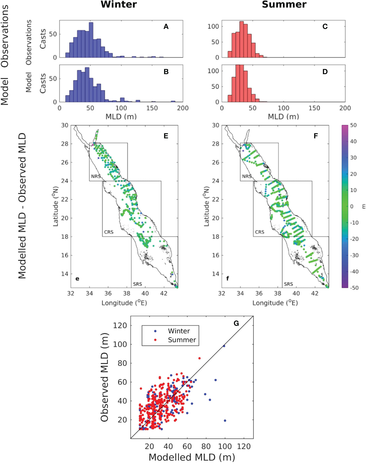
Figure 3 (A, C) Histogram of the number of CTD casts available during the model simulation period (2001−2015) and (B, D) from the daily averaged model output as a function of the MLD; (E, F) the difference between the MLD estimates obtained from the CTD casts and the daily averaged model output; (G) scatter plot of the MLD estimates.

In summer (Figures 3A, B), the MLD from both, measurements and modeling, mostly range between 20 and 40 m, with very few estimates deeper than 60 m. In winter (Figures 3C, D), the model reproduced the observed deepening of the ML (40–60 m). During summer, the MLD exhibit smaller differences along the basin’s central axis (Figure 3E). The largest differences are in the northwestern part of the RS during winter (Figure 3F), where MLD estimates from both the observations and model results are the deepest (data not shown). The RMSD is 13.8 m overall (12.6 m during summer and 15.6 m in winter), with the differences showing a uniform spread in both seasons (Figure 3G). In the CRS, the differences do not exhibit a clear spatial pattern, while local differences may be linked to the higher eddy activity in the region, as well as challenges in simulating the intermediate water pathways in the region (see also Section 3.1). The MLD estimates obtained from the few observations available for the NRS in winter (where most of the deep ML observations are found, Figure 3F) agreed well with the model estimates.

3 Atmospheric buoyancy and momentum fluxes

Surface buoyancy flux and wind stress are important on inducing turbulent mixing and directly impact the development of the ML. We consider the heat and freshwater flux components separately because they generally exhibit different spatial and seasonal variability. The relative importance of the surface buoyancy and momentum fluxes on turbulent mixing is qualitatively assessed by examining the Obukhov length scale. Following the typical geographical partition of the RS (Raitsos et al., 2013; Ahmad and Albarakati, 2015), we consider the two gulfs in the north (GoAq and GoS), the NRS (24°–28°N), the CRS (18°–24°N), and the SRS (between 18°N and the BAM) separately (Figure 1). This partition is based on the mean θ and S characteristics and the unique bathymetric features of each region. For a comprehensive description of the seasonal variability of properties, model results are presented as four-seasons climatology, summer (June–August), autumn (September–November), winter (December–February), and spring (March–May).

3.1 Wind forcing

The seasonal climatology for wind stress in the RS is presented in Figure 4. The wind fields used to force the model simulation in the present study were originally analyzed by Langodan et al. (2017). Because the spatiotemporal characteristics of wind stress closely resemble those of wind field, we only provide a brief overview of the most pertinent features here.

Figure 4

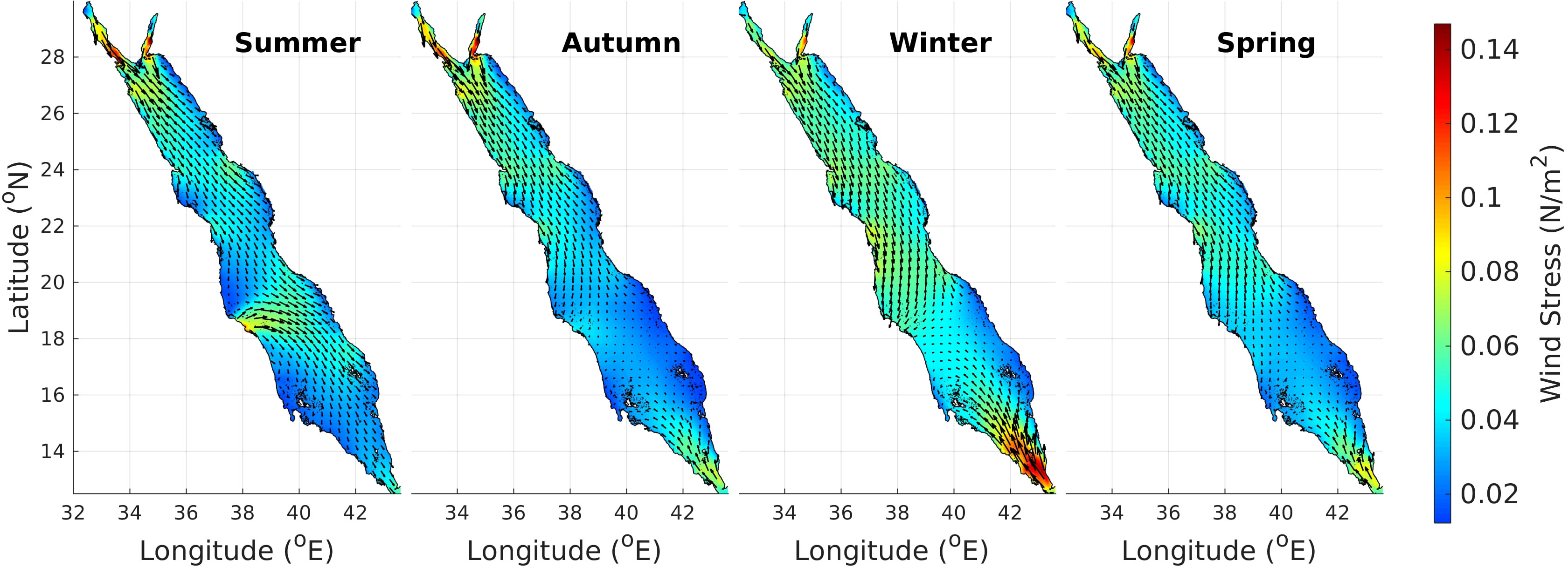
Figure 4 Seasonal climatology for the model estimates of wind stress.

The most prominent feature in the seasonal variability of the wind field is associated with the seasonal reversal of winds in the southern part of the basin, induced by the Indian monsoon system. During the summer, northwesterly winds blow over the entire basin gradually weakening in the south parts of the basin where they reverse during winter (Pratt et al., 1999; Langodan et al., 2017). In winter, wind stress is intensified due to strong and persistent northerly winds especially in the NRS and CRS that are more pronounced along the western parts of the basin. In summer, wind stress is generally reduced in the CRS and NRS, but locally intensifies in the vicinity of gaps in the coastal mountain chains parallel to the RS axis (Jiang et al., 2009; Langodan et al., 2014). Of particular importance are the eastward wind jets that blow through the Tokar Gap in the CRS before shifting to southward towards the eastern part of the SRS.

Wind stress is also amplified by the channeling effect within the elongated Gulf of Aqaba (GoAq) and Gulf of Suez (GoS) in the north and the narrow BAM strait in the south. This leads to intensified wind stress aligned along the axes of the two northern gulf that persists throughout the year, particularly strengthening over their southern parts. Intense wind stress is evident in the vicinity of the BAM strait especially during winter, when northward winds enter through the physical opening of the strait, primarily affecting the western parts of the SRS, reaching with gradually lower intensity the CRS (Pratt et al., 1999; Langodan et al., 2017).

3.2 Surface buoyancy fluxes

The net surface buoyancy flux (B) is the sum of the surface heat and freshwater (FW) flux components and it can be expressed as.

$\begin{array}{ll}B=-ɡ·a_t·\frac{Q}{{\rho }_s·c_p}+ɡ·b_s(E-P)·S,& (1)\end{array}$

where ρ_s is the water density at the surface, g is the gravitational constant (9.81 ms^-2), c_p is the specific heat capacity, a_t and b_s are the thermal expansion and saline contraction coefficients¹* evaluated at the sea surface, and S is the surface salinity. Q is the net heat flux, which is the sum of the net shortwave and longwave radiation, and the sensible and latent heat fluxes. Finally, E denotes evaporation, and P is precipitation. All terms were evaluated using the daily mean model outputs.

The seasonal climatology of the net buoyancy flux and its heat and freshwater flux components are presented in Figure 5. Positive buoyancy fluxes increase the stability of the water column and inhibit vertical mixing, whereas negative buoyancy fluxes reduce stratification and drive convective mixing. The heat and FW fluxes exhibit different seasonal variability and spatial patterns (Figures 5B, C). The seasonal variability of the net buoyancy flux (Figure 5A) is mainly controlled by its heat flux component (Figure 5B), while that of the FW flux component is apparently smaller (Figure 5C). Evaporation is steadily high throughout the year, acting against the near-surface stratification and plays an important role in preconditioning for the deepening of the ML (Sofianos and Johns, 2015).

Figure 5

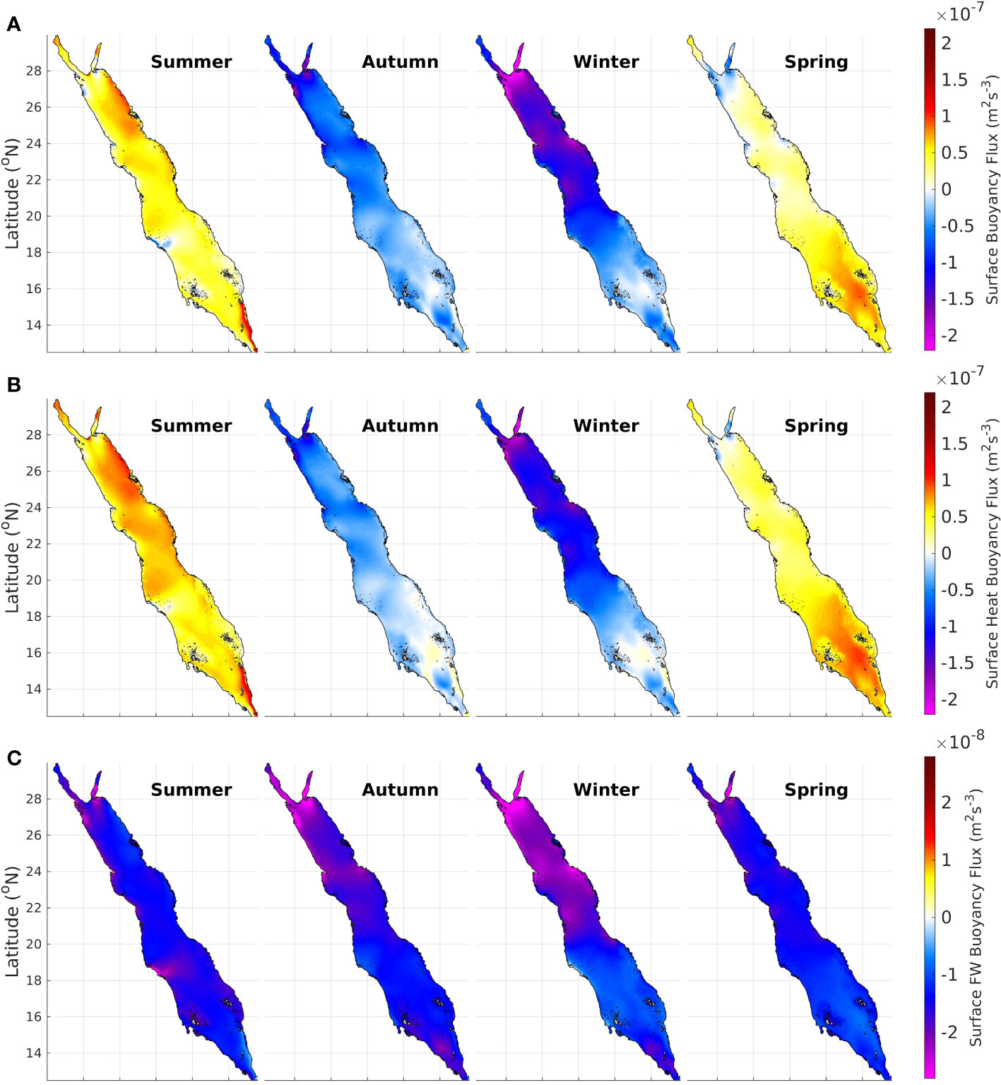
Figure 5 Seasonal climatology for the model estimates of (A) the net air–sea buoyancy flux and its (B) heat flux and (C) freshwater flux components. Positive values indicate a gain in ocean surface buoyancy.

Surface buoyancy loss in the RS starts in early autumn (Figure 5A), predominantly due to surface cooling (Figure 5B). Both heat and FW fluxes exhibit a north–south gradient, with stronger heat and FW losses in the NRS (Figures 5B, C). The highest wintertime surface buoyancy loss occurs in the GoAq, where the monthly mean heat loss can exceed 300 W/m², and evaporation can be as high as 3 my^-1. Although the GoS is located at a similar latitude to the GoAq, the wintertime buoyancy loss is significantly weaker, with the monthly mean heat loss to remain lower than −150 W/m² while the FW flux is less than −1.5 my^-1. These differences reflect the smaller thermal capacity of the GoS due to its shallower depth. Wintertime buoyancy loss is also strong in the northwestern part of the NRS, where the monthly mean heat flux in winter exceeds −250 W/m² and the FW flux is −2.5 my^-1. They are driven by cold air outbreaks that originate in the northwest and by the channeling of northern winds from the two gulfs (Papadopoulos et al., 2022). Locally, increased buoyancy loss near the coasts in the CRS and NRS is driven mostly by the strong surface FW loss (Figures 5A, C), and mainly through evaporation due to the lateral dry winds that blow through the mountain gaps. In contrast to the rest of the RS, the sea surface in the central part of the SRS gains buoyancy even in winter (Figure 5A) as the warmer southerly winds isolate it from the cooler atmospheric systems of the north (Langodan et al., 2017).

In spring, most of the RS gains buoyancy via heating from the atmosphere, especially in the SRS. Buoyancy loss during spring occurs only in the northern RS, in the vicinity of the straits connecting the two gulfs with the open RS, a feature detected also in summer (Figure 5A). In summer, heat (and buoyancy) gain prevails throughout the basin, which is especially strong in the eastern part of the NRS and in the southeastern SRS (Figures 5A, B). Buoyancy loss only appears in the region influenced by the Tokar Jet due to extreme evaporation (Figures 5A, C).

3.3 Relative importance of surface buoyancy and momentum forcing in vertical mixing

To evaluate the relative contribution of wind stress and buoyancy forcing to vertical mixing, we employ the Obukhov length scale, a fundamental parameter introduced by Obukhov (1946) and described in detail by Foken (2006). This scale, denoted as L_m, serves as a universal measure for exchange processes in surface layers, providing insight into the interplay between shearing and buoyancy effects (Phillips, 1977; Large, 1998). It essentially quantifies the relative significance of wind stress versus buoyancy forcing in the turbulent mixing processes responsible for the formation of the ML (Taylor and Ferrari, 2010). The length scale L_m is defined by.

$\begin{array}{ll}{L}_m=\left|\frac{{(U^{*})}^3}{\kappa B}\right|,& (2)\end{array}$

where U^* is the friction (shear) velocity, κ = 0.4 is the von Karman constant, and B is the buoyancy flux. The surface buoyancy flux is estimated as in Equation 1 (Section 4.2) accounting for the individual contribution of its components within the ML. The friction velocity U^* in Eq. 2 represents the contribution of shear on turbulence and is defined as follows.

$$U^{*}=\sqrt{\raisebox{1ex}{$Ws$}\!\left/ \!\raisebox{-1ex}{${\rho }_s$}\right.},$$

where Ws is the wind stress, and ρ_s is the surface density.

This approach allows the quantification of the relative roles of wind-induced shear and buoyancy-driven processes in vertical mixing. Considering the absolute value of the length scale L_m, the buoyancy term B is a measure of the contribution of convective mixing to turbulence when the buoyancy flux is negative or to turbulence suppression when the buoyancy flux is positive (Large, 1998). Practically, the estimates of the length scale L_m represent the depth at which turbulence is more strongly dominated by buoyancy than by wind-induced shear (Taylor and Ferrari, 2010). Because of the nonlinear nature of L_m, local extremes may appear in regions in which B changes its sign and its value reaches zero. As these values indicate the absence of buoyancy forcing, they are removed using a maximum threshold for L_m (<150 m) based on the examination of the distribution of B in daily model outputs, thereby ensuring that other regions were not affected.

The seasonal climatological means for L_m derived from the 2001−2015 model time average show a notable spatiotemporal variability. Nevertheless, characteristic seasonal and spatial patterns emerge (Figure 6). During winter, mixing is mostly controlled by the surface buoyancy fluxes. The strongest buoyant mixing (indicated by small L_m values) appears in the NRS and GoAq, associated with convection (Figure 6). In contrast, wind shear has a higher contribution in other seasons and especially in summer, when buoyancy serves to increase stratification. The impact of wind shear diminishes in winter when convective processes dominate vertical mixing.

Figure 6

Figure 6 Seasonal climatology for the Obukhov length scale.

While buoyancy forcing plays a predominant role in the seasonal variability of L_m, the spatial patterns generally reflect the variability in the wind stress. The strongest contribution of mixing induced by wind shear appears where winds are funneled through straits, such as the two northern gulfs and close to BAM, as well as where jets blow through mountain gaps. In summer, wind forcing dominates mixing in the northern regions of the RS. This is primarily because northern winds are channeled through the narrow gulfs and exit intensified towards the NRS. Wind stress influence is also notable in the western CRS in the Tokar Jet region, with its effects extending into the western part of the SRS, particularly over the shallow regions.

During autumn, the contribution of wind shear gradually diminishes, as buoyancy loss starts to increase everywhere in the RS, especially in the shallow regions of the SRS. In winter, mixing due to wind shear remains strong only in the SRS reflecting the influence of monsoon-driven southern winds that are channeled through the BAM strait.

4 Upper layer circulation

The seasonal climatology for the upper layer circulation in the RS is presented in Figure 7. The general features of the RS circulation have already been described in several previous studies (for example Sofianos and Johns, 2003; Yao et al., 2014a, b; Sofianos and Johns, 2015). Accordingly, we simply provide a brief overview of the most relevant features here.

Figure 7

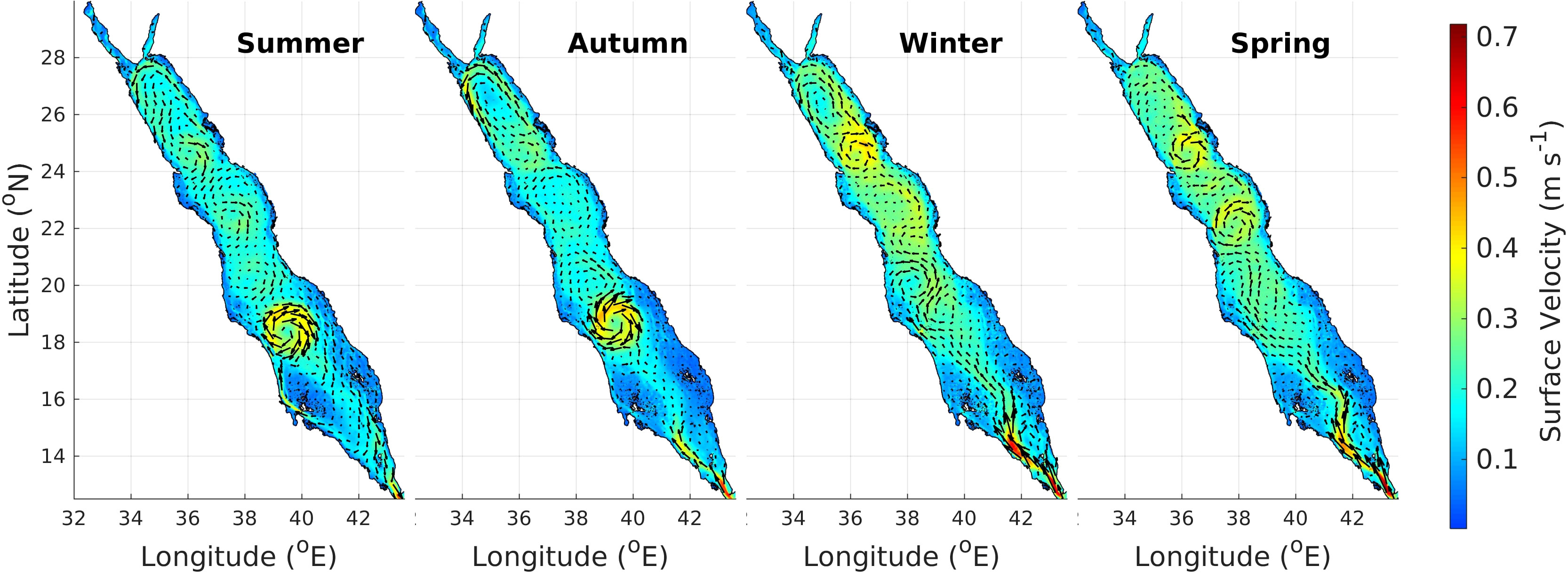
Figure 7 Seasonal climatology of sea surface velocities.

The upper layer circulation of the Red Sea is marked by its seasonal variations, distinctive regional patterns, and the substantial influence of mesoscale eddies. The general flow comprises a northward transport that initially intensifies along the western boundary up to the CRS before it transitions to the eastern shore of the RS and continues up to the NRS through meandering currents and semi-permanent eddies. This upper layer flow is a response to water transformation and sinking processes in the northern parts of the RS that drive a corresponding southward return flow at intermediate and deeper layers that eventually outflow to the GoAden through the BAM strait (Quadfasel and Baudner, 1993; Sofianos and Johns, 2002b; Yao et al., 2014b; Zhai et al., 2015). Mesoscale eddies are present throughout the RS and are particularly frequent in its central region between 18°N and 24°N, where they strengthen in winter (Zhan et al., 2016). Cyclone/anticyclone dipoles also develop in response to lateral wind jets blowing through gaps in the mountains surrounding the RS basin, becoming stronger in summer and spring (Jiang et al., 2009; Langodan et al., 2017; Menezes et al., 2018). The energetic eddies drive strong interactions laterally and with the underlying water masses, while they strongly influence locally the depth of the isopycnals.

The northward upper layer mean flow occurs throughout the year, but intensifies throughout the basin in winter following the reestablishment of the overturning processes. Along this main northward flow several local patterns can be identified. In winter, following the northwesterly reversal of winds in the southern Red Sea, its upper layers are influenced by a surface intrusion of water masses from the Gulf of Aden. This surface flow intensifies along the western boundary of the SRS as it progresses northward before shifting towards the eastern side of the Red Sea. This eastern boundary current transforms into a permanent cyclonic gyre in the NRS, centered between 26°N and 27°N (Sofianos and Johns, 2002b; Yao et al., 2014a). This gyre preconditions this region for intermediate and deep-water formations (Papadopoulos et al., 2015). During summer, the cyclonic gyre that dominates the NRS weakens, while the reestablishment of the northwesterly winds in the south drives an eastern boundary current from the CRS to the SRS. This current primarily contributes to the surface outflow through the BAM, but also partially returns as a northward boundary current along the western coasts. The most striking feature of the summer season is the semi-permanent dipolar eddy that forms in response to the Tokar Jet winds in the CRS, centered at approximately 18.5°N (Bower et al., 2013; Zhai and Bower, 2013; Zhan et al., 2018). In particular the anticyclone in the south is the most energetic eddy in the RS persisting well into Autumn.

5 Seasonal evolution of the MLD

The modeled ML in the RS displays strong seasonal and spatial variability, which closely mirrors the variability of surface forcing while also revealing spatial patterns associated with circulation features. To illustrate these dynamics, we present maps of the seasonal climatology for both mean and maximum MLD in Figure 8. Additionally, monthly spatially averaged values for the individual regions are presented in Figure 9, while detailed monthly climatological maps of the simulated MLD can be found in the Supplementary Material (Supplementary Figure S7). We further explore the influence of the atmospheric buoyancy flux and wind stress on the seasonal MLD evolution by analyzing their daily lagged correlations (Figures 10, Figure 11, respectively).

Figure 8

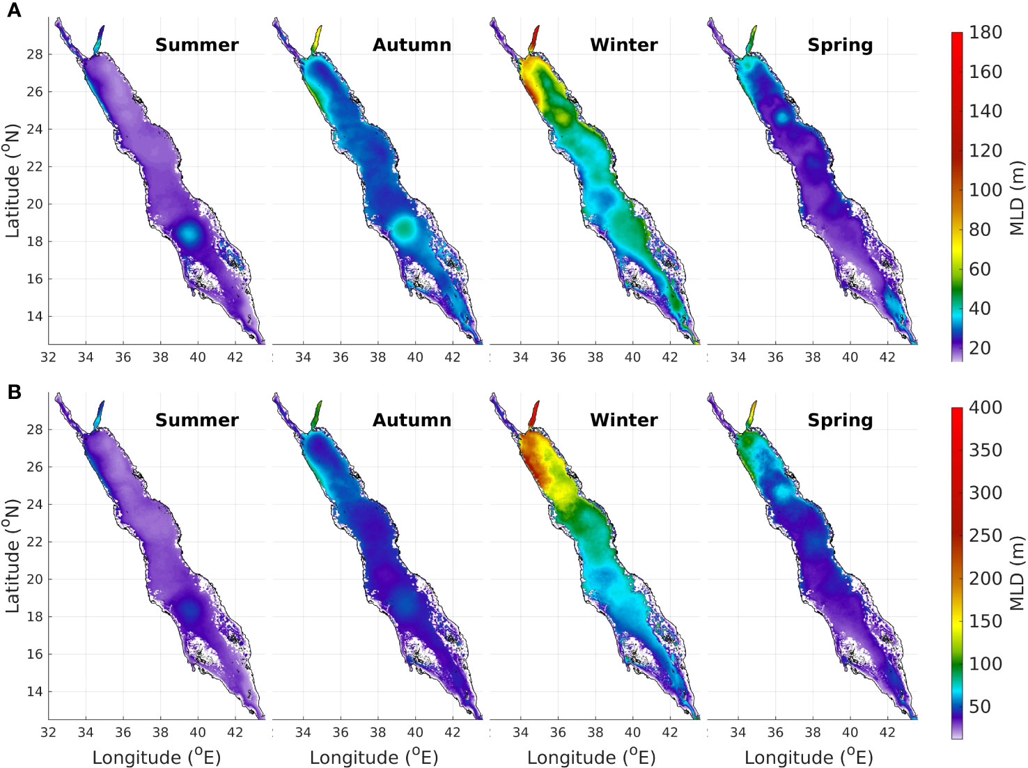
Figure 8 Seasonal climatology of the (A) mean and (B) maximum model MLD estimates.

Figure 9

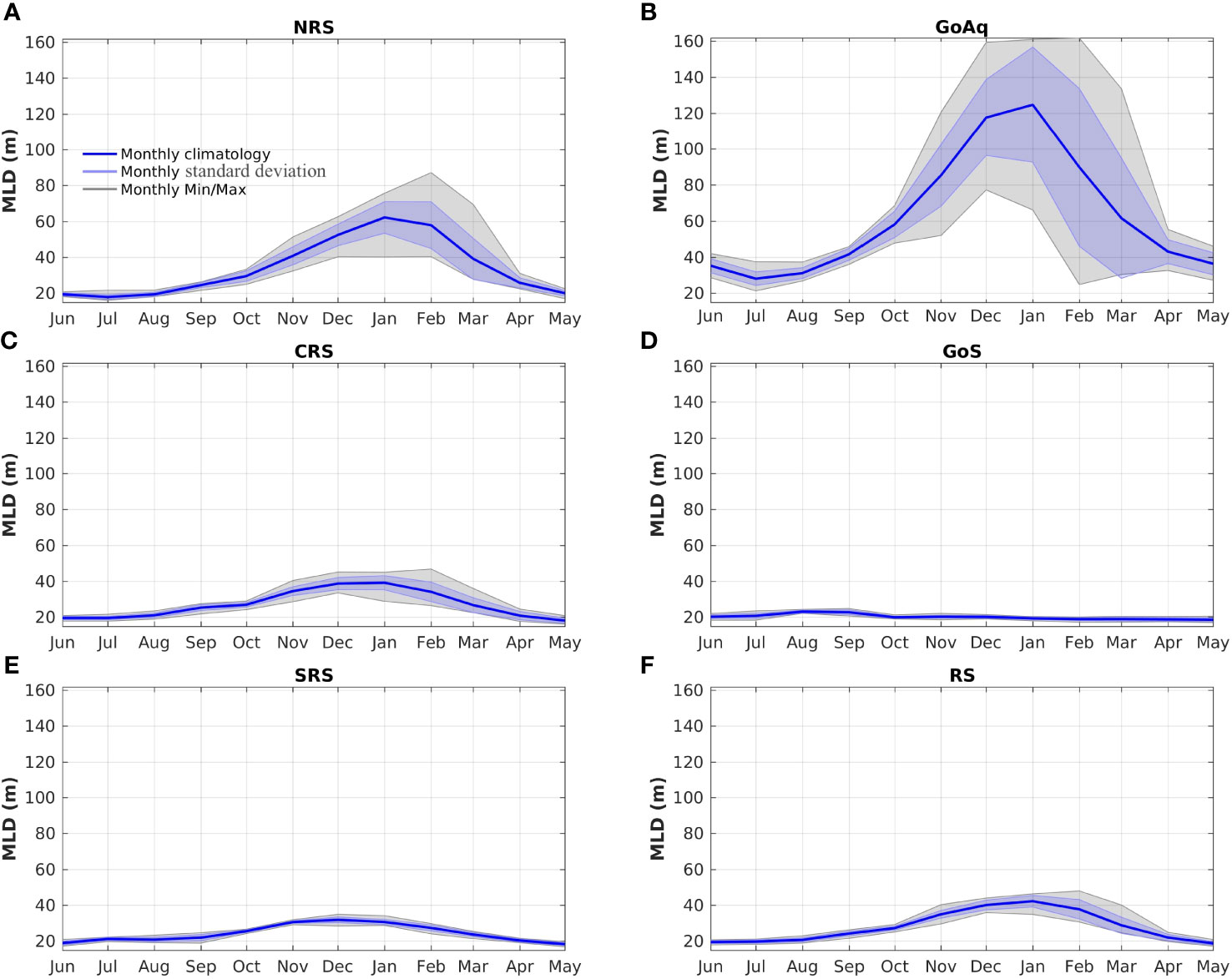
Figure 9 Monthly mean climatology of the simulated MLD during the 2001–2015 period, with the monthly standard deviation and the range between the minimum and maximum monthly mean values averaged over the individual regions: (A) NRS, (B) GoAq, (C) CRS, (D) GoS, (E) SRS, and (F) the entire RS (see Figure 1).

Figure 10

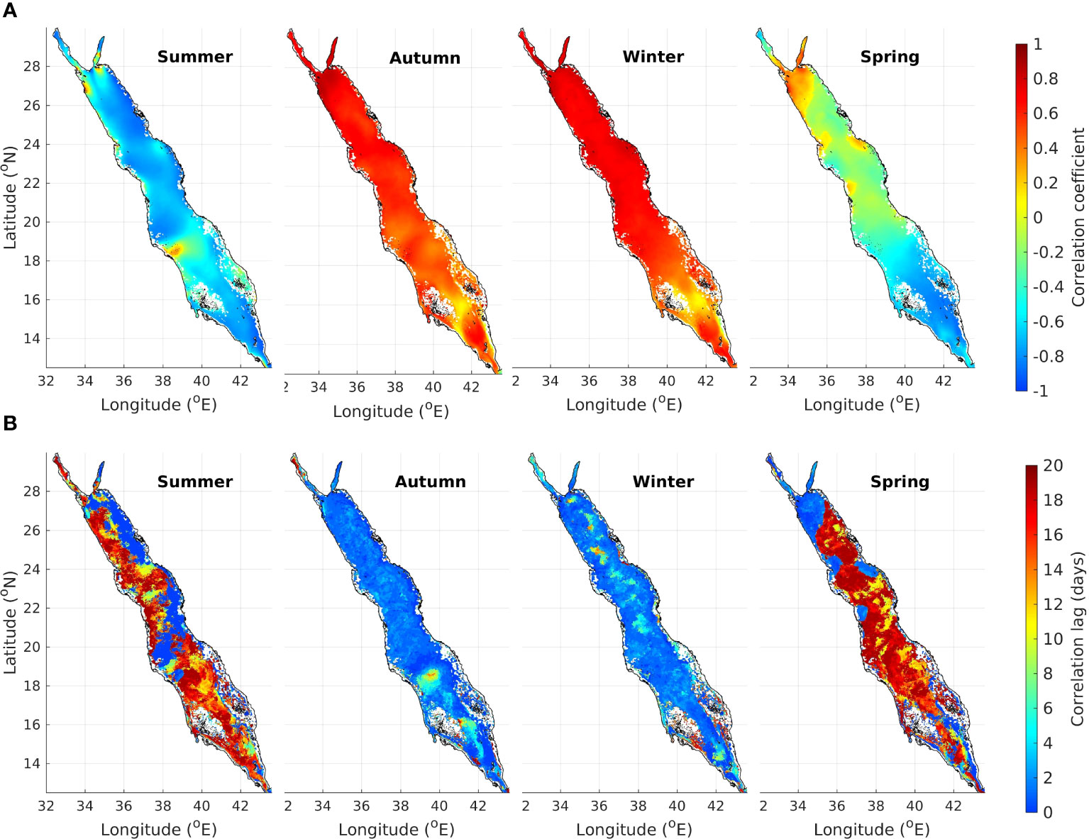
Figure 10 (A) Daily lagged correlation coefficient between MLD and the net air–sea buoyancy flux (B) number of days to reach the maximum correlation coefficient.

Figure 11

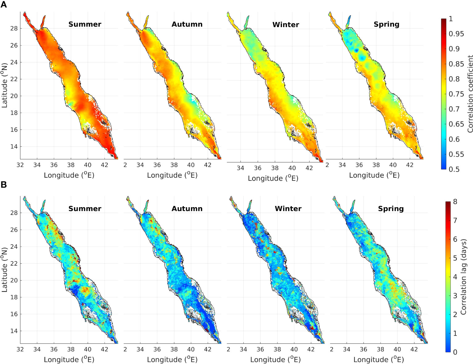
Figure 11 (A) Daily lagged correlation coefficient between MLD and wind stress (B) number of days to reach the maximum correlation coefficient.

In summer, the ML is shallow almost everywhere within the RS (Figure 8), with the exception of local deepening in the southern part of the CRS in the vicinity of the Tokar Jet. The ML starts to deepen in mid-September throughout the basin and the deepest ML is reached in January and February (Figure 9). The ML is deeper in the northern parts of the basin, particularly in the GoAq and the western parts of the NRS (Figure 8). In contrast, it becomes shallower toward the southern parts of the basin, with relative deeper ML found in the eastern parts of the CRS and SRS. In the NRS, the monthly average reach of about 65 m but remain at about 20 m in the SRS. The maximum depth locally reaches over 300 m in the NRS and around 80 m in the SRS. The GoAq exhibits the deepest MLD, with monthly average depths of more than 120 m, while it may locally exceed 400 m (Figure 8B).

Transitioning to early spring, stratification in the near surface layers begins, causing the ML to shoal across the entire basin. During this period, the mean depth remains generally below 30 m (Figure 8A). Nonetheless, it remains relatively deeper in the northern parts of the basin, locally reaching a depth of over 100 m, and in the SRS, particularly near the BAM, locally reaching depths of up to 60 m.

The daily correlations between the MLD and both surface buoyancy and momentum forcing suggest a stronger relation between the large-scale seasonal variability in the MLD and the surface buoyancy flux. Wind forcing shows positive correlation with MLD, whereas buoyancy forcing tends to be positively correlated with MLD during autumn and winter when convection deepens the ML. However, during spring and summer, when heat gain increases stratification, this correlation is negative. Nonetheless, locally the correlation indicates that buoyancy forcing still acts in favor of vertical mixing, especially during spring.

In winter, the correlation with buoyancy forcing is uniformly high (>0.7) in the NRS and CRS (Figure 10A), where the deepest ML is found (Figure 8). In spring, when the thermal stratification shoals the ML throughout the RS, this correlation decreases to approximately 0.3. During summer, the correlation with wind stress is high (>0.8) across the entire RS (Figure 11A), while the correlation with buoyancy forcing is strong (>0.8) only in regions where lateral winds give rise to significant latent heat loss (Figure 10A). In autumn, with the onset of surface buoyancy loss in the northernmost part of the RS, the correlation with buoyancy forcing increases in the two gulfs in the north and in the north and western parts of the NRS. In contrast, the correlation with wind stress is higher in the western parts of the RS. However, in the SRS, especially in the vicinity of the BAM, the correlation with wind stress remains high (>0.8) throughout the year (Figure 11A).

The time lags of reaching the maximum correlation between the forcing components and MLD indicate a faster response of the ML during winter. Wind forcing exhibits relatively short lags, mostly less than 2-3 days. Regarding the buoyancy forcing, MLD responds faster during autumn and winter, generally in less than 2 days, but it exhibits a longer response during spring and summer, in some regions more than 10 days. However, spring and summer are characterized by relatively lower correlation values.

The MLD in the RS exhibits a strong correlation with atmospheric forcing concerning both its temporal and spatial variability. However, when the correlation between the atmospheric components and the MLD is low (often with delayed response), it suggests that other processes may also affect its development that are not explicitly analyzed in this study. For example, wind-generated waves lead to enhanced vertical mixing through wave-induced turbulence, extending the influence to the greater vicinity of regions with intensified winds due to topography. Moreover, lateral transport of heat and salt associated with general and mesoscale circulation play a role in the water column stratification. For example, the northward upper layer flow associated with the general thermohaline circulation in the RS transports warmer and fresher water from the south, which can increase stratification (Krokos et al., 2021). Additionally, the presence of mesoscale eddies may affect the MLD locally by enhancing mixing or vertically displacing isopycnals.

6 Regional characteristics of the MLD

Although different subregions of the Red Sea share similar regimes in terms of seasonal MLD variability and dominant forcing, each subregion has unique characteristics and influences that make them special in their own way. In this regard, we discuss separately the main features of each subregion to allow for a more nuanced understanding of the complex dynamics within the Red Sea.

6.1 Gulf of Aqaba

The ML here is the deepest throughout the year (Figure 8A). During winter, the monthly average MLD in this region can exceed 160 m, and this deep ML shows a longer persistence than in the rest of the RS (Figure 9B). Significant variation in the monthly average MLD in the GoAq indicates that in some years, the ML can become much deeper (Figure 9B). In winter, the MLD has the strongest correlation with surface heat loss (Figure 10A), indicating that this is the primary driver of the deepening of the ML. Spatially, the ML is deepest in the northern part of GoAq, with maximum MLDs locally deeper than 400 m (Figure 8B). Surprisingly, this occurs even though buoyancy forcing and wind stress are more intense in its central and southern parts (Figures 4, 5, respectively). This can be attributed to the inflow of warmer and less saline water from the NRS upper layer, which increases the stratification in the southern part of the gulf and inhibits the development of a deep ML (Krokos et al., 2021). In summer, the monthly average MLD in the GoAq is approximately 30 m. Deeper ML (greater than 50 m) forms in the southern parts of the gulf (Figure 8B) where the MLD exhibits a strong correlation with the intensified winds channeled through the Straits of Tiran, suggesting the dominance of wind-induced mixing (Figure 11A).

6.2 Gulf of Suez

The GoS exhibits a relatively shallow MLD and low seasonal variability due to its shallow depth, which prevents the ML from deepening significantly. Mixing in this area is primarily driven by the wind, except in winter when buoyancy forcing is stronger and exhibits a higher correlation with the MLD (Figures 10A, 11A). However, interestingly, the MLD is slightly shallower in winter than in summer. This suggests that following the intensification of baroclinic circulation in winter, surface inflow of warmer and fresher water from the NRS sustain stratification in the GoS (Sofianos and Johns, 2017), effectively balancing mixing induced by atmospheric forcing.

6.3 North Red Sea

The MLD in the NRS exhibits similar seasonal variations to the GoAq, with the deepest ML occurring in January and February (Figure 9A). This deepening is primarily driven by strong air–sea buoyancy loss during winter (Figure 10A). The ML begins to deepen in autumn, and the correlation between the buoyancy flux and the MLD generally becomes positive and increases (Figure 10A), following the onset of buoyancy loss (Figure 5A). In winter, the monthly MLD averaged over the NRS can exceed 150 m, with a relatively large standard deviation suggesting significant year-to-year variability (Figure 9A). The ML is deeper on the periphery of the NRS (Figure 8A), reaching a maximum depth of more than 250 m (Figure 8B). The NRS experiences a general cyclonic circulation throughout the year, which intensifies in winter (Zhan et al., 2014). In the center of this cyclonic gyre, the ML is shallower due to the doming of the isopycnals. The MLD is also deeper in the western parts of the NRS throughout the year, especially during the winter months (Figure 8A) with several factors contributing to this variability. First, wind forcing is consistently stronger in the western parts throughout the year (Figure 11). In autumn and winter, the ML is deepest in the regions with the greatest buoyancy flux (Figure 5A), which also occurs in the western parts of the basin (Figure 8A). Additionally, the eastern parts of the NRS are directly influenced by the warmer and fresher water advected from the south in the upper layers following the general cyclonic circulation (Krokos et al., 2021). This water increases stratification and leads to the shallowing of the ML in this region. In the southern part of the NRS (toward the CRS), the MLD distribution is affected by a semi-permanent anticyclone at approximately 25°N, leading to a noticeable deepening of the local ML (Figure 8A), with a maximum MLD exceeding 150 m (Figure 8B). At this location, the local MLD has a low correlation with atmospheric forcing (Figures 10A, 11A), suggesting that MLD is mostly associated with the presence of the anticyclone.

In spring, the MLD generally becomes shallower to less than 30 m, except in the western part of the NRS and in the vicinity of the straits connecting with the two northern gulfs. The mean MLD in these regions is about 50 m, while the maximum depth may exceed 100 m. In the vicinity of the straits of the two gulfs in the north, the correlation of the MLD with buoyancy fluxes is higher than with wind stress (Figures 10A, Figure 11A), suggesting that the deepening of the ML is sustained by the evaporative heat flux and convective mixing. In summer, the ML is generally shallow, with mean values less than 30 m. A deeper ML is still found in its western parts, where the correlation with wind stress is higher, and the MLD may exceed 50 m along the western coast (Figure 8B).

6.4 Central Red Sea

The deepest ML in the CRS occurs mainly along the central axis of the basin and at its eastern parts (Figure 8A). It is generally shallower compared to the NRS, with a monthly mean ML depth typically less than 50 m, and the maximum depth generally shallower than 120 m. During winter, the region experiences weaker surface buoyancy loss compared to northern areas (Figure 8B), but buoyancy still shows a notable correlation with the MLD (Figure 10A). Wind stress, on the other hand, exhibits a higher correlation with the MLD in its eastern part increasing towards the south (Figure 11). The general northward flow of the upper layer advects warmer and less saline water from the south, initially following a westward path that results in a shallower MLD in the western parts of the CRS. However, advection influence gradually shifts toward the northeast (Krokos et al., 2021).

In summer, the ML in the CRS is generally shallow, with mean values typically less than 20 m (Figure 8A). The maximum depth reaches about 40 m (Figure 8B), except in the south region around 18°N, where a strong anticyclone forms in response to the Tokar Jet winds. This leads to a local deepening of the ML to more than 60 m (Figure 8B). This anticyclone is part of a dipole eddy system, with the cyclone in the north having a weaker but still noticeable influence on the MLD. The MLD in this region is strongly correlated with wind stress over the Tokar anticyclone, and its effects extend to the eastern part of the CRS (Figure 11A). However, the correlation between the MLD and the buoyancy flux is generally weak across this region (Figure 10A). In contrast, the correlation with buoyancy forcing is higher in the area where the cyclonic eddy persists. It is worth noting that even though the Tokar Jet winds cease in early September (Jiang et al., 2009), the semi-permanent dipole eddy system remains for longer, imprinted in the ML until October (see Supplementary Material, Supplementary Figure S8).

6.5 South Red Sea

In the SRS, the ML is generally shallower compared to other parts of the basin (Figure 9E). During summer, the ML is confined to a thin upper layer, typically within the first 20 m. However, in its western sections, it can be slightly deeper, locally reaching down to 30 m. This shallow depth is attributed to a combination of two main factors: the intense surface heat gain and the southward movement of warmer and saline surface water from the CRS (Krokos et al., 2021). Both of these factors favor higher stratification in the region. The depth of this upper layer is also confined by the subsurface intrusion of fresher and cooler GAIW. During this period, the SRS experiences strong southward winds that have a stronger correlation with the MLD compared to buoyancy flux (Figures 10A, 11A). Additionally, these southward winds induce coastal upwelling along the eastern boundary south of 17°N (Sofianos et al., 2002). This is consistent with the spatial pattern of the ML in the SRS, which also shows a gradual increase from east to west.

With the reversal of the monsoon in September, warmer and fresher surface water from the GoAd enters the RS through the BAM. This mainly affects the western parts of the SRS, leading to increased stratification and shallowing of the MLD (Krokos et al., 2021). Additionally, the prevailing northward winds during winter induce downwelling along the eastern coast of the SRS (Sofianos and Johns, 2002b). Consequently, the ML becomes relatively deeper, reaching depths of 80 m in the eastern part of the SRS (Figure 8B). The deepest part of the ML is restricted to the central part of the SRS, bounded by extended coastal shallow areas on both sides of the region (Figure 8A). The MLD in this area has a stronger correlation with the southern winds entering the RS through the BAM (Figure 11A). Buoyancy forcing, on the other hand, has a weaker correlation (Figure 10A) due to the weak surface heat loss in the SRS during winter (Figure 8B). This increase in MLD, particularly near the BAM, continuous until April (see Supplementary Material, Supplementary Figure S8). In May, various factors contribute to the shallowing of the ML, including the gradual weakening of the southern winds, the intensification of the surface heat gain, and the reestablishment of the southward transport of warmer surface water from the north part of the SRS.

7 Summary and discussion

Surface mixing is a fundamental process for the ecosystem’s functioning in the Red Sea, strongly impacting the basin’s physical and biochemical characteristics. This study provides a comprehensive description of the seasonal and spatial evolution of the ML in the RS and highlights the relative roles of wind and buoyancy forcing. The analysis is based on a 15-year high resolution numerical simulation that has been extensively validated against available observations endorsing its capability to replicate seasonal temperature and salinity variations in the upper layer, as well as key features of RS circulation patterns and their spatiotemporal changes. The MLD estimates, obtained using the relative variance method introduced by Huang et al. (2018) applied on potential density, align well with observations, both for summer and winter conditions.

The analysis of MLD seasonal variability reveals significant spatiotemporal fluctuations, overcoming the drawback of studying MLD in the RS using sparse data from various locations and years. The ML tends to be very shallow during summer almost everywhere in the RS, with an average depth of approximately 20 m. However, the simulation reveals localized noteworthy deepening near the Straits of Tiran in the Gulf of Aqaba (GoAq), the western NRS (deeper than 50 meters locally), and the western SRS (around 50 meters). Deeper ML is also observed in the southern part of the Central Red Sea (CRS) associated with the Tokar anticyclone. Gradual deepening of the ML initiates in early autumn and extends until late March, with peaks in January and February throughout the RS. The deepest MLs appear in the western NRS and the GoAq. In these regions, monthly mean MLD can be deeper than 180 meters, with local maxima exceeding 250 meters in the NRS and 400 meters in the GoAq. Notably, there is significant interannual variability in the MLD, with some years experiencing considerably deeper ML.

Examination of the impact of the atmospheric forcing components to vertical mixing reveals that seasonal variability is primarily influenced by the surface buoyancy fluxes, especially their heat component. Although freshwater fluxes in the RS region dominate the annually averaged surface buoyancy forcing, their seasonal variability is too weak to significantly affect the seasonal variability of the total buoyancy flux. It is worth noting that, due to the cumulative effect of wintertime surface buoyancy loss, the ML in the RS is deepest after the peak in the surface heat loss. On the other hand, wind-induced mixing contribution is more significant during summer and spring when buoyancy forcing acts to increase the stratification. The relatively deep ML in the northern parts of the basin (NRS and the GoAq) and in the SRS near the BAM also correlates strongly with the wind stress, indicating its influence. In autumn, the wind contribution gradually decreases as buoyancy loss starts to increase everywhere within the RS and convective processes become the dominant driver of vertical mixing. Wind-driven mixing remains relatively strong only in the SRS due to strong winds channeled through the BAM. However, strong winds also induce local buoyancy loss, which deepens the MLD through convective mixing.

This analysis, following previous literature, considered different subregions of the RS based on their mean characteristics and distinct bathymetric features. Although they exhibit unique characteristics and influences, some similar regimes in terms of seasonal MLD variability and dominant forcing are also apparent. In terms of spatial MLD variability, the most characteristic feature is the strong north-south gradient, indicative of the stronger buoyancy forcing in the northern parts of the basin, especially during winter. The northern parts of the basin exhibit the deepest MLDs that persist for a longer period compared to the rest of the basin. Similarities between different regions appear in the vicinity of the narrow and shallow straits connecting the subbasins, the BAM strait in the south and the straits connecting the RS with the two Gulfs in the north. Exchanges of waters through the straits have a strong impact on the upper layer physical properties and may inhibit the effect of atmospheric forcing. Moreover, these regions are all strongly influenced by wind induced mixing, which usually exceeds that of buoyancy forcing, due to the intensification of winds through the narrow topography surrounding the straits.

Despite the generally high correlation between the MLD and the atmospheric forcing components, its temporal and spatial variability may also be influenced by advective fluxes, such as lateral advection of heat and salt, local upwelling and downwelling processes, as well as by wave induced mixing. While this study mainly focuses on the air-sea buoyancy and momentum forces and their impact on the MLD, it further acknowledges the influence of thermohaline circulation and mesoscale activity, and the potential role of wave-induced turbulence, distinguishing the intricate interplay between surface air–sea interactions and internal processes in shaping the MLD variability in the RS.

Data availability statement

The data analyzed in this study is subject to the following licenses/restrictions: The datasets generated during and/or analyzed during the current study are available from the corresponding author on reasonable request. Requests to access these datasets should be directed to GK, g.krokos@hcmr.gr.

Author contributions

GK: Conceptualization, Data curation, Investigation, Methodology, Visualization, Writing – original draft, Formal Analysis, Funding acquisition, Validation. IC: Investigation, Methodology, Writing – review and editing, Conceptualization. PZ: Writing – review and editing. VP: Writing – review and editing. MH: Methodology, Supervision, Writing – review and editing, Investigation. IH: Conceptualization, Methodology, Supervision, Writing – review and editing, Funding acquisition, Resources.

Funding

The author(s) declare that financial support was received for the research, authorship, and/or publication of this article. The research reported in this publication was supported by King Abdullah University of Science and Technology (KAUST) under the Competitive Research Grant Program (CRG), Grant #UFR/1/2979-01-01.

Acknowledgments

Model simulations and postprocessing of the outputs were performed at the KAUST supercomputing facility in Shaheen-II, Saudi Arabia. We are grateful to the KAUST HPC team for their valuable support during the generation and processing of the model outputs. We also thank the UK MetOffice Ocean for providing the Operational SST and Sea Ice Analysis (OSTIA) products. OSTIA data are available from the Copernicus Marine Environmental Monitoring Service (CMEMS) web portal (http://marine.copernicus.eu/).

Conflict of interest

The authors declare that the research was conducted in the absence of any commercial or financial relationships that could be construed as a potential conflict of interest.

Publisher’s note

All claims expressed in this article are solely those of the authors and do not necessarily represent those of their affiliated organizations, or those of the publisher, the editors and the reviewers. Any product that may be evaluated in this article, or claim that may be made by its manufacturer, is not guaranteed or endorsed by the publisher.

Supplementary material

The Supplementary Material for this article can be found online at: https://www.frontiersin.org/articles/10.3389/fmars.2024.1342137/full#supplementary-material

Footnotes

1. ^ * Coefficients c_p, a_t, and b_s are computed using the Gibbs-Sea Water (GSW) Oceanographic Toolbox (McDougall and Barker, 2011).

References

Abdulla C. P., Alsaafani M. A., Alraddadi T. M., Albarakati A. M. (2018). Mixed layer depth variability in the Red Sea. Ocean. Sci. 14, 563–573. doi: 10.5194/os-14-563-2018

CrossRef Full Text | Google Scholar

Acker J., Leptoukh G., Shen S., Zhu T., Kempler S. (2008). Remotely-sensed chlorophyll a observations of the northern red sea indicate seasonal variability and influence of coastal reefs. J. Mar. Syst. 69, 191–204. doi: 10.1016/j.jmarsys.2005.12.006

CrossRef Full Text | Google Scholar

Ahmad F., Albarakati A. M. A. (2015). “Heat balance of the Red Sea,” in The Red Sea: The Formation, Morphology, Oceanography and Environment of a Young Ocean Basin. Eds. Rasul N. M. A., Stewart I. C. F. (Springer Berlin Heidelberg, Berlin, Heidelberg), 355–361. doi: 10.1007/978-3-662-45201-1_21

CrossRef Full Text | Google Scholar

Albarakati A. M. A., Ahmad F. (2013). Variation of the surface buoyancy flux in the Red Sea. Indian J. Mar. Sci. 42, 717–721.

Google Scholar

Alexander M. A., Scott J. D., Deser C. (2000). Processes that influence sea surface temperature and ocean mixed layer depth variability in a coupled model. J. Geophys. Res.: Oceans. 105, 16823–16842. doi: 10.1029/2000jc900074

CrossRef Full Text | Google Scholar

Bower A. S., Swift S. A., Churchill J. H., Mccorkle D. C., Abualnaja Y., Limeburner R., et al. (2013). New observations of eddies and boundary currents in the Red Sea, 15, 9875. In. EGU. Gen. Assembly. Conf. Abstracts. 15, 9875.

Google Scholar

Carlson D. F., Fredj E., Gildor H. (2014). The annual cycle of vertical mixing and restratification in the Northern Gulf of Eilat/Aqaba (Red Sea) based on high temporal and vertical resolution observations. Deep-Sea. Res. Part I.: Oceanogr. Res. Papers. 84, 1–17. doi: 10.1016/j.dsr.2013.10.004

CrossRef Full Text | Google Scholar

Carton J. A., Grodsky S. A., Liu H. (2008). Variability of the oceanic mixed layer 1960-2004. J. Climate 21, 1029–1047. doi: 10.1175/2007JCLI1798.1

CrossRef Full Text | Google Scholar

Carvalho S., Kürten B., Krokos G., Hoteit I., Ellis J. (2019). “The Red Sea,” in World Seas: an Environmental Evaluation (Academic Press, Elsevier), 49–74. doi: 10.1016/B978-0-08-100853-9.00004-X

CrossRef Full Text | Google Scholar

Cember R. P. (1988). On the sources, formation, and circulation of Red Sea deep water. J. Geophys. Res. 93, 8175. doi: 10.1029/JC093iC07p08175

CrossRef Full Text | Google Scholar

Cerovečki I., Marshall J. (2008). Eddy modulation of air–sea interaction and convection. J. Phys. Oceanogr. 38, 65–83. doi: 10.1175/2007jpo3545.1

CrossRef Full Text | Google Scholar

Cronin M. F., Sprintall J. (2008). Wind- and buoyancy-forced upper ocean. Encyclopedia. Ocean. Sci., 337–345. doi: 10.1016/B978-012374473-9.00624-X

CrossRef Full Text | Google Scholar

de Boyer Montégut C., Madec G., Fischer A. S., Lazar A., Iudicone D. (2004). Mixed layer depth over the global ocean: An examination of profile data and a profile-based climatology. J. Geophysical Res. C: Oceans 109, 1–20. doi: 10.1029/2004JC002378

CrossRef Full Text | Google Scholar

Dee D. P., Uppala S. M., Simmons A. J., Berrisford P., Poli P., Kobayashi S., et al. (2011). The ERA-Interim reanalysis: Configuration and performance of the data assimilation system. Q. J. R. Meteorol. Soc. 137, 553–597. doi: 10.1002/qj.828

CrossRef Full Text | Google Scholar

Denman K. L., Gargett A. E. (1995). Biological–physical interactions in the upper ocean: the role of vertical and small scale mixing processes. Annu. Rev. Fluid. Mechanics. 27, 225–255.

Google Scholar

Dong S., Sprintall J., Gille S. T., Talley L. (2008). Southern Ocean mixed-layer depth from Argo float profiles. J. Geophys. Res. 113, C06013. doi: 10.1029/2006JC004051

CrossRef Full Text | Google Scholar

Dong C., McWilliams J. C., Liu Y., Chen D. (2014). Global heat and salt transports by eddy movement. Nat. Commun. 5, 1–6. doi: 10.1038/ncomms4294

CrossRef Full Text | Google Scholar

Eladawy A., Nadaoka K., Negm A., Abdel-Fattah S., Hanafy M., Shaltout M. (2017). Characterization of the northern Red Sea’s oceanic features with remote sensing data and outputs from a global circulation model. Oceanologia 59, 213–237. doi: 10.1016/j.oceano.2017.01.002

CrossRef Full Text | Google Scholar

Foken T. (2006). 50 years of the monin-obukhov similarity theory. Boundary Layer Meteorol 119, 431–447. doi: 10.1007/s10546-006-9048-6

CrossRef Full Text | Google Scholar

Gaube P., McGillicuddy D. J., Moulin A. J. (2018). Mesoscale eddies modulate mixed layer depth globally. Geophys. Res. Lett. doi: 10.1029/2018GL080006

CrossRef Full Text | Google Scholar

Gittings J. A., Raitsos D. E., Kheireddine M., Racault M. F., Claustre H., Hoteit I. (2019). Evaluating tropical phytoplankton phenology metrics using contemporary tools. Sci. Rep. 9, 1–10. doi: 10.1038/s41598-018-37370-4

CrossRef Full Text | Google Scholar

Gittings J. A., Raitsos D. E., Krokos G., Hoteit I. (2018). Impacts of warming on phytoplankton abundance and phenology in a typical tropical marine ecosystem. Sci. Rep. 8. doi: 10.1038/s41598-018-20560-5

CrossRef Full Text | Google Scholar

Huang P.-Q., Lu Y.-Z., Zhou S.-Q. (2018). An objective method for determining ocean mixed layer depth with applications to WOCE Data. J. Atmospheric. Oceanic. Technol. 35, 441–458. doi: 10.1175/JTECH-D-17-0104.1

CrossRef Full Text | Google Scholar

Jiang H., Farrar J. T., Beardsley R. C., Chen R., Chen C. (2009). Zonal surface wind jets across the Red Sea due to mountain gap forcing along both sides of the Red Sea. Geophys. Res. Lett. 36, 1–6. doi: 10.1029/2009GL040008

CrossRef Full Text | Google Scholar

Kantha L., Clayson C. A. (2002). Ocean mixed layer. Encyclopedia. Atmospheric. Sci., 291–298.

Google Scholar

Kara A. B. (2003). Mixed layer depth variability over the global ocean. J. Geophys. Res. 108, 1–15. doi: 10.1029/2000jc000736

CrossRef Full Text | Google Scholar

Krokos G., Cerovečki I., Papadopoulos V. P., Hendershott M. C., Hoteit I. (2021). Processes governing the seasonal evolution of mixed layers in the Red Sea. J. Geophys. Res.: Oceans., 1–18. doi: 10.1029/2021jc017369

CrossRef Full Text | Google Scholar

Langodan S., Cavaleri L., Vishwanadhapalli Y., Pomaro A., Bertotti L., Hoteit I. (2017). The climatology of the Red Sea – part 1: the wind. Int. J. Climatol. 37, 4509–4517. doi: 10.1002/joc.5103

CrossRef Full Text | Google Scholar

Langodan S., Cavaleri L., Viswanadhapalli Y., Hoteit I. (2014). The Red Sea: A natural laboratory for wind and wave modeling. J. Phys. Oceanogr. 44, 3139–3159. doi: 10.1175/JPO-D-13-0242.1

CrossRef Full Text | Google Scholar

Large W. G. (1998). Modeling and parameterizing the ocean planetary boundary layer. Ocean. Modeling. Parameterization., 81–120. doi: 10.1007/978-94-011-5096-5_3

CrossRef Full Text | Google Scholar

Lorbacher K., Dommenget D., Niiler P. P., Köhl A. (2006). Ocean mixed layer depth: A subsurface proxy of ocean-atmosphere variability. J. Geophys. Res.: Oceans. 111, 1–22. doi: 10.1029/2003JC002157

CrossRef Full Text | Google Scholar

Mann K. H., Lazier J. R. N. (1991). Dynamics of marine ecosystems, biological–physical interactions in the oceans (Boston: Blackwell Scientific Publications), 466.

Google Scholar

McDougall T. J., Barker P. M. (2011). Getting started with TEOS-10 and the gibbs seawater (GSW) oceanographic toolbox, 28pp. SCOR/IAPSO. WG127.

Google Scholar

Menezes V. V., Farrar J. T., Bower A. S. (2018). Westward mountain-gap wind jets of the northern Red Sea as seen by QuikSCAT. Remote Sens. Environ. 209, 677–699. doi: 10.1016/j.rse.2018.02.075

CrossRef Full Text | Google Scholar

Morcos S. A. (1982). The Egyptian expedition to the Red Sea 1934/35, (Article 247).

Google Scholar

Neumann A. C., McGill D. A. (1961). Circulation of the Red Sea in early summer. Deep. Sea. Res. 8, 223–235. doi: 10.1016/0146-6313(61)90023-5

CrossRef Full Text | Google Scholar

Obukhov A. M. (1946). ‘Turbulentnost’ v temperaturnoj–neodnorodnoj atmosfere (Turbulence in an atmosphere with a non-uniform temperature)’. Trudy Inst. Theor. Geofiz.

Google Scholar

Papadopoulos V. P., Krokos G., Dasari H. P., Abualnaja Y., Hoteit I. (2022). Extreme heat loss in the Northern Red Sea and associated atmospheric forcing. Front. Mar. Sci. 9. doi: 10.3389/fmars.2022.968114

CrossRef Full Text | Google Scholar

Papadopoulos V. P., Zhan P., Sofianos S., Raitsos D. E., Qurban M., Abualnaja Y., et al. (2015). Factors governing the deep ventilation of the Red Sea. J. Geophys. Res.: Oceans. 120, 7493–7505. doi: 10.1002/2015JC010996

CrossRef Full Text | Google Scholar

Patzert W. C. (1974). Wind-induced reversal in Red Sea circulation. Deep-Sea. Res. Oceanogr. Abstracts. 21, 109–121. doi: 10.1016/0011-7471(74)90068-0

CrossRef Full Text | Google Scholar

Phillips O. M. (1966). On turbulent convection currents and the circulation of the Red Sea. Deep. Sea. Res. Oceanogr. Abstracts. 13, 1149–1160. doi: 10.1016/0011-7471(66)90706-6

CrossRef Full Text | Google Scholar

Phillips O. M. (1977). The dynamics of the upper ocean, Vol. 61. 223–247.

Google Scholar

Pratt L. J., Johns W., Murray S. P., Katsumata K. (1999). Hydraulic interpretation of direct velocity measurements in the Bab al Mandab. J. Phys. Oceanogr. 29, 2769–2784. doi: 10.1175/1520-0485(1999)029<2769:HIODVM>2.0.CO;2

CrossRef Full Text | Google Scholar

Privett D. W. (1959). Monthly charts of evaporation from the N. Indian Ocean (including the Red Sea and the Persian Gulf). Q. J. R. Meteorol. Soc. 85, 424–428. doi: 10.1002/qj.49708536614

CrossRef Full Text | Google Scholar

Quadfasel D., Baudner H. (1993). Gyre-scale circulation cells in the Red Sea. Oceanol. Acta 4), 221–229.

Google Scholar

Raitsos D. E., Pradhan Y., Brewin R. J. W., Stenchikov G., Hoteit I. (2013). Remote sensing the phytoplankton seasonal succession of the Red Sea. PloS One 8, e64909. doi: 10.1371/journal.pone.0064909

CrossRef Full Text | Google Scholar

Rasul N. M. A., Stewart I. C. F., Nawab Z. A. (2015). “Introduction to the Red Sea: Its origin, structure, and environment,” in The Red Sea: The Formation, Morphology, Oceanography and Environment of a Young Ocean Basin. Eds. Rasul N. M. A., Stewart I. C. F. (Springer Berlin Heidelberg, Berlin, Heidelberg), 1–28. doi: 10.1007/978-3-662-45201-1_1

CrossRef Full Text | Google Scholar

Silverman J., Gildor H. (2008). The residence time of an active versus a passive tracer in the Gulf of Aqaba: A box model approach. J. Mar. Syst. 71, 159–170. doi: 10.1016/j.jmarsys.2007.06.007

CrossRef Full Text | Google Scholar

Sofianos S. S., Johns W. E. (2002b). An Oceanic General Circulation Model (OGCM) investigation of the Red Sea circulation, 1. Exchange between the Red Sea and the Indian Ocean. J. Geophys. Res. 107. doi: 10.1029/2001JC001184

CrossRef Full Text | Google Scholar

Sofianos S. S., Johns W. E. (2003). An Oceanic General Circulation Model (OGCM) investigation of the Red Sea circulation: 2. Three-dimensional circulation in the Red Sea. J. Geophys. Res. 108, 3066. doi: 10.1029/2001JC001185

CrossRef Full Text | Google Scholar

Sofianos S. S., Johns W. E. (2007). Observations of the summer Red Sea circulation. J. Geophys. Res. 112, 1–20. doi: 10.1029/2006JC003886

CrossRef Full Text | Google Scholar

Sofianos S. S., Johns W. E. (2015). The Red Sea: Water Mass Formation, Overturning Circulation, and the Exchange of the Red Sea with the Adjacent Basins. Eds. Rasul N. M. A., Stewart I. C. F. (Berlin, Heidelberg: Springer Berlin Heidelberg). doi: 10.1007/978-3-662-45201-1

CrossRef Full Text | Google Scholar

Sofianos S. S., Johns W. E. (2017). The summer circulation in the Gulf of Suez and its influence in the Red Sea thermohaline circulation. J. Phys. Oceanogr. 47, 2047–2053. doi: 10.1175/jpo-d-16-0282.1

CrossRef Full Text | Google Scholar

Sofianos S. S., Johns W. E., Murray S. P. (2002). Heat and freshwater budgets in the Red Sea from direct observations at Bab el Mandeb. Deep-Sea. Res. Part II.: Topical. Stud. Oceanogr. 49, 1323–1340. doi: 10.1016/S0967-0645(01)00164-3

CrossRef Full Text | Google Scholar

Taylor J. R., Ferrari R. (2010). Buoyancy and wind-driven convection at mixed layer density fronts. J. Phys. Oceanogr. 40, 1222–1242. doi: 10.1175/2010JPO4365.1

CrossRef Full Text | Google Scholar

Tragou E., Garrett C., Outerbridge R., Gilman C. (1999). The heat and freshwater budgets of the Red Sea. J. Phys. Oceanogr. 29, 2504–2522. doi: 10.1175/1520-0485(1999)029<2504:THAFBO>2.0.CO;2

CrossRef Full Text | Google Scholar

Viswanadhapalli Y., Dasari H. P., Langodan S., Challa V. S., Hoteit I. (2017). Climatic features of the Red Sea from a regional assimilative model. Int. J. Climatol. 37, 2563–2581. doi: 10.1002/joc.4865

CrossRef Full Text | Google Scholar

Weatherall P., Marks K. M., Jakobsson M., Schmitt T., Tani S., Arndt J. E., et al. (2015). A new digital bathymetric model of the world’s oceans. Earth Space Sci. 2, 331–345. doi: 10.1002/2015EA000107

CrossRef Full Text | Google Scholar

Wolf-Vecht A., Paldor N., Brenner S. (1992). Hydrographic indications of advection/convection effects in the Gulf of Elat. Deep. Sea. Res. Part A. Oceanogr. Res. Papers. 39, 1393–1401. doi: 10.1016/0198-0149(92)90075-5

CrossRef Full Text | Google Scholar

Xie J., Krokos G., Sofianos S., Hoteit I. (2019). Interannual variability of the exchange flow through the Strait of Bab-al-Mandeb. J. Geophys. Res.: Oceans. 124, 1988–2009. doi: 10.1029/2018JC014478

CrossRef Full Text | Google Scholar

Yao F., Hoteit I., Pratt L. J., Bower A. S., Köhl A., Gopalakrishnan G., et al. (2014b). Seasonal overturning circulation in the Red Sea: 2. Winter circulation. J. Geophys. Res.: Oceans. 119, 2263–2289. doi: 10.1002/2013JC009331

CrossRef Full Text | Google Scholar

Yao F., Hoteit I., Pratt L. J., Bower A. S., Zhai P., Kohl A., et al. (2014a). Seasonal overturning circulation in the Red Sea: 1. Model validation and summer circulation. J. Geophys. Res.: Oceans. 119, 2238–2262. doi: 10.1002/2013JC009004

CrossRef Full Text | Google Scholar

Zhai P., Bower A. S. (2013). The response of the Red Sea to a strong wind jet near the Tokar Gap in summer. J. Geophys. Res.: Oceans. 118, 422–434. doi: 10.1029/2012JC008444

CrossRef Full Text | Google Scholar

Zhai P., Pratt L. J., Bower A. S. (2015). On the crossover of boundary currents in an idealized model of the Red Sea. J. Phys. Oceanogr. 150318154651004. doi: 10.1175/JPO-D-14-0192.1

CrossRef Full Text | Google Scholar

Zhan P., Gopalakrishnan G., Subramanian A. C., Guo D., Hoteit I. (2018). Sensitivity studies of the Red Sea eddies using adjoint method. J. Geophys. Res.: Oceans. 123, 8329–8345. doi: 10.1029/2018JC014531

CrossRef Full Text | Google Scholar

Zhan P., Krokos G., Guo D., Hoteit I. (2019). Three-dimensional signature of the Red Sea eddies and eddy-induced transport. Geophys. Res. Lett. 46, 2167–2177. doi: 10.1029/2018GL081387

CrossRef Full Text | Google Scholar

Zhan P., Subramanian A. C., Yao F., Hoteit I. (2014). Eddies in the Red Sea: A statistical and dynamical study. J. Geophys. Res.: Oceans. 119, 3909–3925. doi: 10.1002/2013JC009563

CrossRef Full Text | Google Scholar

Zhan P., Subramanian A. C., Yao F., Kartadikaria A. R., Guo D., Hoteit I. (2016). The eddy kinetic energy budget in the Red Sea. J. Geophys. Res.: Oceans. 121, 4732–4747. doi: 10.1002/2015JC011589

CrossRef Full Text | Google Scholar

Zhan P., Guo D., Krokos G., Dong J., Duran R., Hoteit I. (2022). Submesoscale processes in the upper red sea. J. Geophys Res. Oceans 127, 1–17. doi: 10.1029/2021JC018015

CrossRef Full Text | Google Scholar