Mapping seabird vulnerability to offshore wind farms in Norwegian waters

Introduction: Offshore wind energy development (OWED) has been identified as a major contributor to the aspired growth in Norwegian renewable energy production. Spatially explicit vulnerability assessments are necessary to select sites that minimize the harm to biodiversity, including seabird populations. Distributional data of seabirds in remote areas are scarce, and to identify vulnerable areas, species, and seasons it is necessary to combine data sets and knowledge from different sources.

Methods: In this study, we combined seabird tracking data, data from dedicated coastal and seabird at-sea surveys, and presence-only data from citizen science databases to develop habitat suitability maps for 55 seabird species in four seasons throughout the Norwegian exclusive economic zone; in total 1 million km² in the Northeast Atlantic. The habitat suitability maps were combined with species-specific vulnerability indicators to yield maps of seabird vulnerability to offshore wind farms (OWFs). The resulting map product can be used to identify the relative vulnerability of areas prospected for OWED with respect to seabird collision and habitat displacement. More detailed assessments can be done by splitting the spatial indicators into seasonal and species-specific components.

Results and discussion: Associated with higher diversity of seabirds near the coast, the cumulative vulnerability indicator showed a strong declining gradient from the coast to offshore waters while the differences in vulnerability between ocean areas and seasons were negligible. Although the present map product represents the best currently available knowledge, the indicators are associated with complex uncertainties related to known and unknown sampling biases. The indicators should therefore be used cautiously, they should be updated regularly as more data become available, and we recommend that more detailed environmental impact assessments based on dedicated seabird surveys, tracking of birds from potentially affected populations and population viability analyses are conducted in areas ultimately selected for OWED.

1 Introduction

Offshore wind energy development (OWED) has been identified as a major contributor to the aspired growth in Norwegian renewable energy production before 2030, and potential areas for OWED have been suggested in 20 marine areas comprising 55,371 km² in the Norwegian exclusive economic zone (EEZ) (NVE, 2023). However, Norwegian waters hold significant proportions of European seabird populations (Fauchald et al., 2015), and the impact of offshore wind farms (OWFs) on seabirds through collision, disturbance and habitat displacement (Garthe and Hüppop, 2004; Furness et al., 2013) is accordingly a major environmental concern. As a first step in a strategic environmental assessment, a spatially explicit vulnerability analysis of seabirds that potentially could be affected by OWED is necessary to select sites that minimize the harm to vulnerable seabird populations (Croll et al., 2022).

To achieve a precise and unbiased strategic assessment of OWED, detailed knowledge with respect to the spatial distribution and the potential consequences of OWF are needed for all seabird populations present in the assessment area. However, datasets that document a species’ spatial distribution, the impact of OWF on its vital rates and the consequences for population dynamics are rare. One solution is to restrict the analyses to a few well-studied species and monitoring sites with the implicit assumption that this selection is a representative sample of the seabird populations in the assessment area. However, discarding species or areas based on data scarcity could result in an assessment bias towards well studied species and data rich areas (e.g., Halpern and Fujita, 2013).

One strategy to mitigate assessment bias related to data availability is to combine all available datasets as well as expert assessments into composite indicators (e.g., Halpern et al., 2008, Halpern et al., 2012; Issaris et al., 2012). The philosophy behind this approach is to synthesize the best available knowledge of all relevant components of the system into indicators using a transparent framework consisting of a set of procedures with associated assumptions (Halpern and Fujita, 2013). Procedures often involve the use of expert opinions to systematically weigh the importance and impacts of stressors and environmental components, specification of algorithms for correcting sampling bias and methodological discrepancies, and statistical modelling for spatial and temporal interpolations (Halpern and Fujita, 2013). Using “best available knowledge” means that the indicator should be updated regularly as more insight of the system, more data, and improved statistical methods become available. The indicator approach has gained traction in recent years as large open-access databases, fast computing, and programing environments for data management and statistical modeling have improved and become increasingly available (for assessments of birds and wind farms see e.g., Bradbury et al. (2014); Kelsey et al. (2018); Goodale et al. (2019); Perrow (2019); Cleasby et al. (2020); May et al. (2020); May et al. (2021)).

Here, we use the indicator approach to develop a data product for vulnerability assessment of marine birds (including seabirds, marine ducks and geese) in the Norwegian EEZ with respect to OWED. Spatial datasets on marine birds in the area are limited, and we used a combination of seabird tracking data, survey data and citizen science data to develop standardized habitat suitability maps in four seasons for relevant marine birds in the assessment area. The habitat suitability maps were combined with indicators of species-specific vulnerability with respect to collision with wind turbines and displacement from OWF areas (Garthe and Hüppop, 2004; Furness et al., 2013; Robinson Willmott et al., 2013; Dierschke et al., 2016) to yield spatially explicit species-specific vulnerability indicators (Bradbury et al., 2014; Kelsey et al., 2018). Wind farms can also attract seabirds such as gulls, cormorants and shags by providing roosting opportunities and enhanced feeding conditions due to e.g., “reef effects” (Vanermen et al., 2015; Dierschke et al., 2016). Effects of attraction are not explicitly considered in the present indicators; however, it should be noted that attraction could represent both a negative effect through increased collision risk as well as positive effects through e.g., enhanced food availability (Vanermen et al., 2015).

The indicators were summed into a cumulative vulnerability map for marine birds in the assessment area. Our approach builds on the methods developed by Garthe and Hüppop (2004) and Furness et al. (2013) for quantifying species-specific vulnerability, and on Bradbury et al. (2014) and Kelsey et al. (2018) for distributing the vulnerability scores in the assessment area using spatial models of seabird distribution. As a further refinement of Bradbury et al. (2014) and Kelsey et al. (2018), our approach combines different data sources to model habitat suitability, making it possible to assess the vulnerability of relevant species in the entire assessment area.

2 Materials and methods

The workflow of analyses is shown in Figure 1. Seabird observation data and environmental data were combined in species distribution models (SDMs) to yield maps of habitat suitability for each species and season. From the literature, data on conservation status and vulnerability with respect to OWF were compiled and combined to OWF vulnerability scores. From the vulnerability scores and habitat suitability models, vulnerability maps were calculated for each species and season. The maps were combined and normalized to the minimum - maximum values in the assessment area to yield a map product comprising three levels of detail: Maps of vulnerability of each species and season; maps of seasonal vulnerability for all species combined; and a map of total seabird vulnerability.

Figure 1

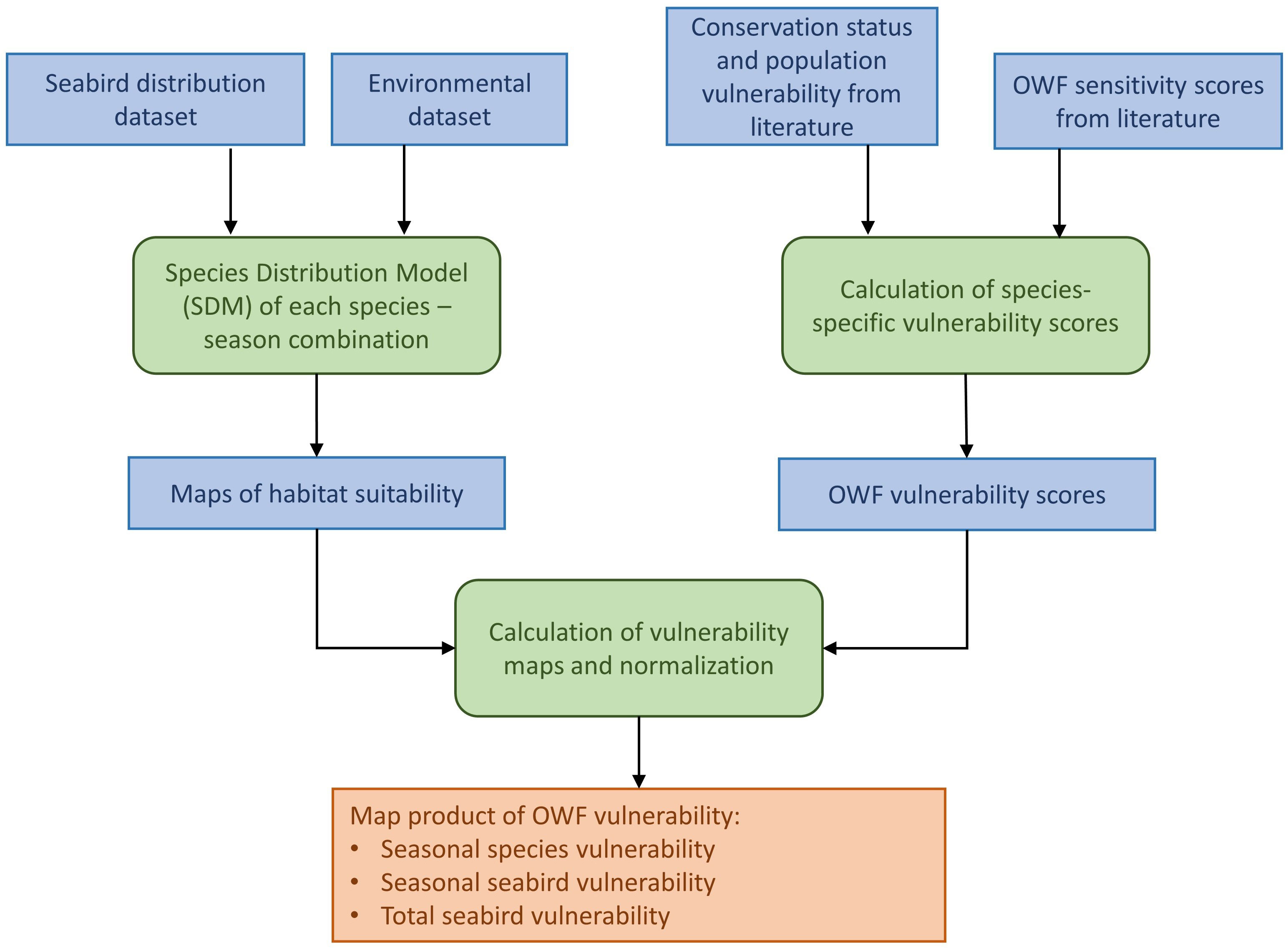
Figure 1 Workflow, including input data sets (blue boxes) and analyses (green boxes) to obtain a map product of seabird vulnerability to offshore wind farms (OWF).

2.1 Study area and species

The assessment area for the vulnerability analyses was defined by the Norwegian EEZ, which extends from the coastline of the Norwegian mainland and 200 nautical miles offshore, comprising an area of 1 million km² in the Northeast Atlantic (Figure 2). Within this area, assessment units were defined by the cells in a 10x10 km² regular grid (WGS 84/UTM zone 33N, EPSG:32633) often used in environmental assessments of offshore energy development in Norway.

Figure 2

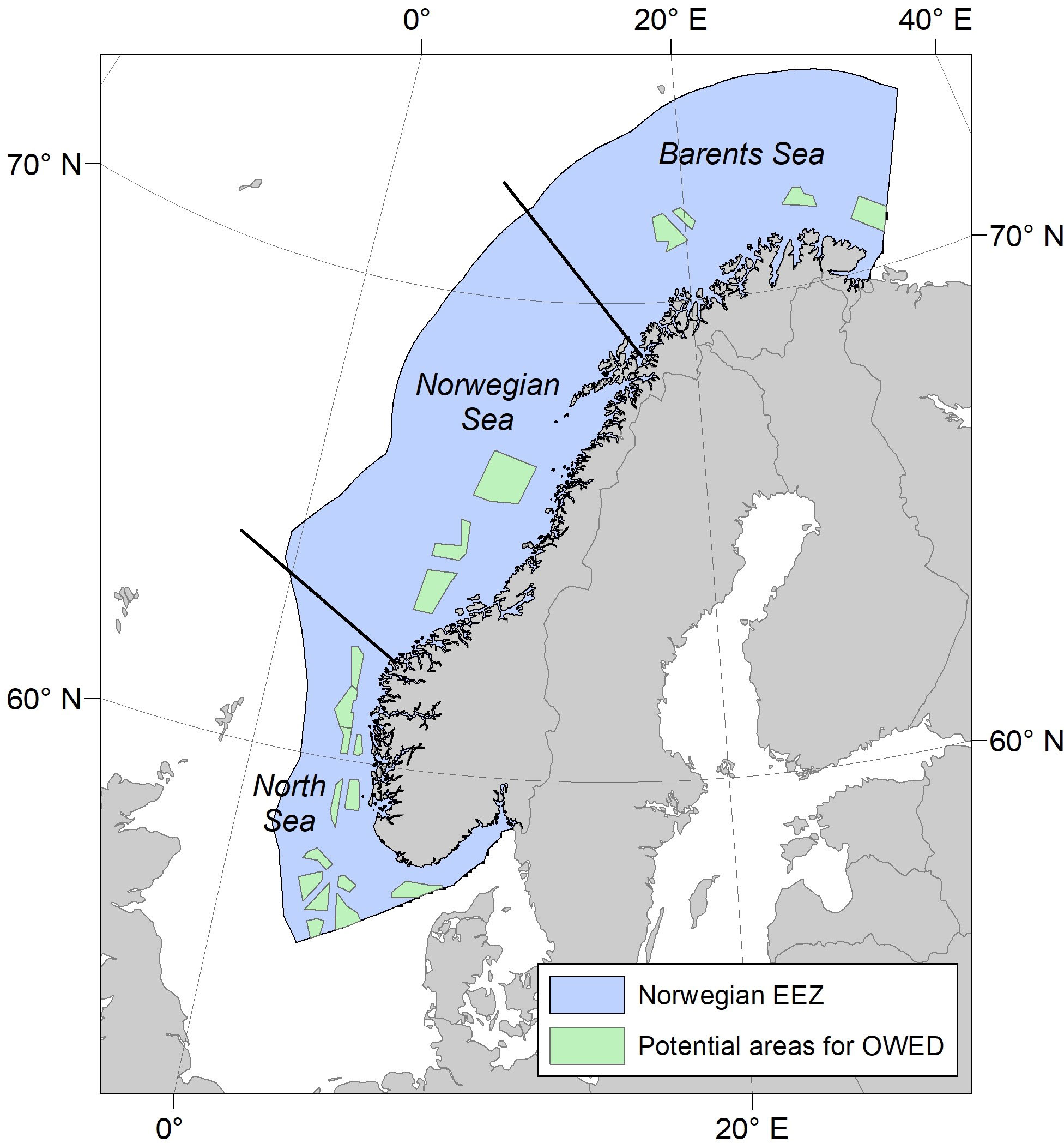
Figure 2 Study area. The study area was defined by the Norwegian exclusive economic zone (EEZ) (blue area). Green areas are areas proposed for further evaluation with respect to development of offshore wind energy. Delineation of the Barents Sea, Norwegian Sea and North Sea is indicated by lines.

Following the definition of Croxall et al. (2012), seabirds are defined as “species for which a large proportion of the total population rely on the marine environment for at least part of the year”. Globally, Dias et al. (2019), identified 359 extant species that met this criterion. From this list, we identified 53 species that according to our datasets (see section 2.2 below) were regularly observed in the study area. In addition to these 53 “true” seabird species, we added 13 bird species that, in at least part of the year, were observed in Norwegian marine and coastal areas and therefore could be affected by OWFs. The total list of 66 species is given in Supplementary Table 1.

Analyses were conducted separately for four seasons chosen to approximate the annual cycle of seabirds in the area: Spring, migration period (February-April); Summer, breeding period (May-July); Autumn, moulting and migration period (August-October); and Winter, winter period (November-January).

The number of observations for some species and seasons were too low to provide reliable estimates of habitat suitability from the species distribution models (SDMs); i.e., the models did not converge or provided unreliable predictions. Note that the lower threshold of sample size for a reliable SDM depends on the spatial distribution of observations and the threshold did therefore vary among models. For 11 relatively rare species, we were not able to model habitat suitability in any season and these species were accordingly removed from the assessment, giving a final list of 55 species (Supplementary Table 1).

2.2 Habitat suitability maps

Habitat suitability maps for six of the seabird species were compiled from the NEAS dataset (section 2.2.1). For the rest of the species, habitat suitability was estimated using SDMs developed according to the target group (TG) method (Phillips et al., 2009). The observations of each species were modelled by environmental variables, and habitat suitability was predicted for each cell in the assessment area. The SDMs were based on three datasets with spatial explicit observations of marine birds in the study area. These datasets were: seabird at-sea survey data (section 2.2.2); systematic coastal survey data (section 2.2.3); and citizen science presence-only data (section 2.2.4).

All analyses were conducted using the R Statistical language version 4.2.3 (R Core Team, 2023).

2.2.1 NEAS dataset

For six species (Atlantic fulmar (Fulmarus glacialis), black-legged kittiwake (Rissa tridactyla), thick-billed murre (Uria lomvia), common murre (Uria aalge), little auk (Alle alle) and Atlantic puffin (Fratercula arctica)), maps of habitat suitability were collected from the NEAS dataset. The NEAS dataset was developed by the SEATRACK program (SEATRACK, 2023) and is based on tracking data of 2356 birds using geolocation (GLS) loggers in 25 seabird colonies in the Northeast Atlantic. The dataset and methods are described in detail in Fauchald et al. (2021). In short, the maps combine SDMs based on tracking data of birds from the network of seabird colonies with data on population sizes to provide monthly maps of densities of birds from Northeast Atlantic colonies. The dataset covers 87% of the Northeast Atlantic populations, however in Norwegian waters this coverage is even higher, and close to 100%. From the NEAS dataset, density values for the six pelagic species were retrieved for the Norwegian EEZ and average estimates for each cell and season were calculated.

2.2.2 Seabirds at-sea data

Data from seabirds at-sea surveys were retrieved from the ESAS (European Seabirds at Sea) database (ESAS, 2022) and from the SEAPOP seabird at-sea dataset (Fauchald, 2011). SEAPOP is the national monitoring program for seabirds in Norway. The seabirds at-sea data were collected through standardized strip transect sampling where individuals of all bird species were counted from the bridge of a ship in a 300 m wide strip while the ship was steaming at a constant speed and direction (Tasker et al., 1984). Species that are commonly attracted to ships (e.g., fulmars and gulls), and therefore over-estimated in strip transect sampling, were counted as point observations at regular time intervals (most commonly every 10 minutes). Small and diving species (e.g., auks) are more difficult to detect or might avoid the ship and their abundance is therefore often under-estimated in at-sea surveys. In the analyses, observations were not corrected for distance to ship.

In total, seabirds at-sea data contributed with 120,717 observations of individual marine birds within the study area (Figure 3A). The dataset covered the entire study area however, inshore coastal areas and fjords generally had a low coverage and the large offshore areas of the Norwegian Sea had a lower coverage than the Barents Sea and the North Sea.

Figure 3

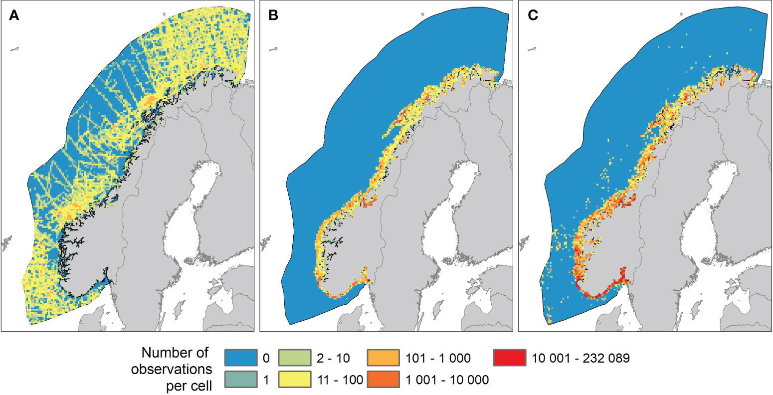
Figure 3 Datasets used in species distribution modeling (SDMs). Maps show number of observations of seabirds in 10x10 km² cells in the study area from three datasets: (A) Seabirds at sea data, (B) coastal survey data, and (C) citizen science data.

2.2.3 Coastal survey data

Coastal survey data on seabirds were retrieved from the SEAPOP database (SEAPOP, 2023). This dataset consists of data from systematic mapping and monitoring of marine birds in specified areas or locations along the Norwegian coast and Svalbard. Observations were made from small boats, by UAVs, airplanes or on foot. The dataset includes counts of breeding populations as well as systematic counts of migrating, molting and wintering birds. In total, this dataset comprised 256,610 observations of individual marine birds in the study area (Figure 3B). All observations were made inshore with a particularly high coverage in permanent monitoring plots along the coast.

2.2.4 Citizen science data

Finally, seabird observations were retrieved from the Norwegian national species observations system (Artsobs, 2023). This database is a collection of data from many different sources. Species are registered to lowest taxonomic level together with parameters such as behavior, observer id, method, time and position. BirdLife Norway has contributed with a large number of standardized high-quality observations, and we included only observations registered as a part of BirdLife’s activity. For the Norwegian EEZ, this dataset comprised 3,965,542 observations of individual marine birds (Figure 3C). Almost all observations were found along the coast, with “hot spots” in areas with high density and activity of bird watchers.

2.2.5 Environmental data

We included seven environmental variables in the SDMs:

1. Depth. Depth is an important parameter determining marine productivity and the availability of food for seabirds. Bottom depth is particularly important for benthic feeding birds such as cormorants and sea ducks. Depth data were retrieved from the ETOPO 1 Global Relief Model (Amante and Eakins, 2009) developed by National Geophysical Data Center (NGDC), an office of the National Oceanic and Atmospheric Administration (NOAA). From the dataset, the average depth was calculated for each cell in the assessment area.

2. Slope. Bottom topography is important for physical oceanographic processes generating productive areas such as fronts and up-welling areas that attract seabirds. From the depth data, we calculated the slope in depth in the 8-cell neighborhood of each cell in the assessment area using the terrain function in the terra package in R (Hijmans, 2023).

3. SST. Sea-surface temperature (SST) is often a good predictor for the habitats of marine species. We retrieved the Daily Optimum Interpolation Sea Surface Temperature (DOISST) Version 2.1 provided by the National Oceanic and Atmospheric Administration (NOAA) (Huang et al., 2021) and assigned each cell in the assessment area with an average value for each season.

4. TGrad. The spatial gradient in sea surface temperature reflects fronts where different water masses meet. Such areas are often productive and might attract foraging seabirds. Using the SST data, we calculated the “gradient” in SST in the 8-cell neighborhood of each cell in the assessment area using the terrain function in the terra package in R (Hijmans, 2023).

5. SSS. Sea surface salinity is an important environmental parameter affecting biological productivity and the habitats of coastal marine birds. SSS varies with the distance to land, the strength of the coastal current and the runoff from land. SSS data from surface waters (< 5 meters) were retrieved from the CTD (conductivity, temperature, and depth) dataset hosted by the ICES data portal (ICES Data Portal, 2022). Average interpolated SSS values for each season were calculated for each cell in the assessment area.

6. DFCoast. The distance from coast is important for biological production, availability and selection of food items, the exposure to wind and waves and not least the birds’ connection to their breeding locations. Distance from coast was calculated for each cell in the assessment area.

7. DACoast. The Norwegian coastal current runs close to the coast from the Swedish border in southeast to the Russian border in northeast. It forms an important bio-climatic gradient and is responsible for the dispersion of plankton along the coast. To mirror this bio-climatic gradient, the distance along the coast was calculated for each cell in the assessment area as the projected distance along a line running along the coast from southeast to northeast.

Several of the environmental variables describe, at least partly, similar physical or biological features. There was accordingly a strong collinearity between DACoast and SST (Pearson’s |r| = 0.93) and a collinearity between Depth, Slope, SSS and DFCoast (Pearson’s |r| ranging from 0.51 to 0.73) (Supplementary Table 2). However, for several models, removal of variables due to collinearity reduced the models’ ability to predict presences. We therefore decided to include all variables in the initial models and subsequently remove variables to optimize model performance and parsimony. In other words, although the collinearity among the variables is likely to preclude the interpretation of the relationship between bird observations and specific environmental features, we prioritized the model prediction accuracy over the interpretability of the spatial predictors (Legendre and Legendre, 2012).

2.2.6 Sampling bias and the target group approach

While seabirds at-sea data have a standardized registration of sampling effort, the coastal dataset includes several different observation methods with different measures of effort, and the citizen science data are “presence-only” data with no information of observer effort. Consequently, it was not feasible to correct for any direct measures of observer effort in the analyses, and all datasets were aligned to the “presence-only” format.

The observations in the resulting dataset were highly biased with “hot spots” along the coast with more than 10,000 seabird observations per cell, and remote offshore cells with zero or only a few observations (Figure 3). To reduce the effect of a skewed sampling effort we decided to randomly subsample each dataset to a maximum of 1000 observations per cell.

Due to heterogeneous sampling effort (Figure 3), a random selection of background or pseudo-absence points would create biases towards areas with high sampling intensity (Elith and Leathwick, 2009). To control for heterogeneous sampling effort, we used the Target Group (TG) approach suggested by (Phillips et al., 2009). Instead of using a random or regular sampling of background points as a contrast to the presences, the TG method uses the observations of other species within the same species group (TG). In principle, this means that the TG method introduces the same bias in the background points as is present in the observations. It has been shown that the TG method efficiently removes sampling biases in SDMs (e.g., Barber et al., 2022). However, areas with high density of other species within the target group will also give a higher number of background points, resulting in an under-estimation of habitat suitability in areas with high biodiversity or abundance of the target group (Ranc et al., 2017; Vollering et al., 2019).

To control for some of the spatial heterogeneity in diversity, the species were divided into two target groups; (1) strictly coastal species, and (2) species that can be found both offshore and along the coast. The Target Groups are defined in Supplementary Table 1.

2.2.7 Species distribution models (SDMs)

Except for the species from the NEAS dataset (section 2.2.1), SDMs were conducted for all identified marine bird species (section 2.1; Supplementary Table 1). For each species and season, the relationship between the species observations and environmental variables was analyzed using the cells in the assessment area as the unit of analysis. In line with the TG approach, the response variable was defined as the proportion of the number of observations of the analyzed species (number of presences) and the sum of observations of other species (number of background points). A logistic model was used to fit the relationship between the response variable and the environmental variables. We used GAM (Generalized Additive Model), where the response is modeled as a combination of non-lineal smooth functions to account for non-linear relationships (Wood, 2017). Several modelling methods are regularly used in SDMs (Norberg et al., 2019). In the present study, we fitted 196 models of relatively large datasets (> 50,000 observations) and efficiency with respect to computation and interpretation, as well as flexibility in model formulation were important. GAM is a computationally efficient and well-proven method with straightforward interpretation and built-in regularization of the predictor function to avoid overfitting (Wood, 2017). We used thin-plate regression splines as smoothers and the optimal degree of smoothing was determined by Generalized Cross-validation (GCV). In cases when the model did not converge or produced unrealistic predictions due to over-fitting, the complexity of the model was constrained by specifying a maximum number of knots in the smooth function and/or removing environmental variables from the model. All analyzes and predictions were conducted using the terra package (Hijmans, 2023) and the mgcv package (Wood, 2017) in R.

The initial model was formulated as:

$\begin{array}{ll}gam(Presence/Backround)~s(Depth)+s(Slope)+s(SST)+s(TGrad)+s(SSS)+DFCoast+s(DACoast), family=binomial& (1)\end{array}$

2.2.8 Calculation of habitat suitability

Based on the predicted presence from the SDMs Equation 1 or NEAS dataset, habitat suitability was calculated in the assessment area for each species and season. The predicted presences were standardized to the season with the highest sum of predicted presence in the assessment area. Thus, habitat suitability c in cell i in season j was calculated as:

$\begin{array}{ll}{c}_{i,j}=n\times \frac{p_{i,j}}{ma{x}_j{\sum }_i{p}_{i,j}}& (2)\end{array}$

Where n is the number of cells in the assessment area and p is the predicted values from the SDM or predicted density values from the NEAS dataset.

Note that habitat suitability Equation 2 is standardized to the season with highest predicted presence, meaning that habitat suitability is independent of the general abundance or rarity of the species but will vary geographically and seasonally according to how the species migrate in and out of the assessment area.

2.3 Species-specific vulnerability

The calculation of species-specific vulnerability to OWF was based on the methods developed by Garthe and Hüppop (2004) and refined by Furness et al. (2013); Bradbury et al. (2014) and Kelsey et al. (2018). The vulnerability indicator combines three factors considered important for seabirds’ vulnerability to OWF: (1) conservation status, (2) direct impact of OWF through increased mortality due to collisions with wind turbines, and (3) indirect impact of OWF through habitat disturbance causing birds to avoid the impacted area. The indicators are scaled from 1 (least vulnerable) to 5 (most vulnerable).

Indicator values were either based on published data (Garthe and Hüppop, 2004; King et al., 2009; Furness et al., 2013; Robinson Willmott et al., 2013; Dierschke et al., 2016) or assessments made by an international expert group (named in Furness et al. (2013)). For species for which there was insufficient information, we used values ​​from closely related and comparable species. Indicator values and references are given in Supplementary Tables 3–5.

2.3.1 Conservation status

The general vulnerability of seabird populations to acute or indirect mortality is related to factors such as population size, population trends and demography. Garthe and Hüppop (2004); Furness et al. (2013); and Bradbury et al. (2014) used the unweighted average of scores from (1) biogeographical population size, (2) threat status, and (3) adult survival as an indicator of conservation status. In accordance with this, but specific to the Norwegian context, we included: (1) National (Norwegian) proportion of the European population (a), (2) red list status on the Norwegian red list (b), and (3) adult survival (c) to define conservation status (CS):

$\begin{array}{ll}CS=\frac{a+b+c}{3}& (3)\end{array}$

The Norwegian proportion of the European population (a) was based on the number of breeding individuals in Norway (incl. Svalbard) retrieved from the Norwegian red list for species (Artsdatabanken, 2022) and the number of breeding individuals in Europe obtained from BirdLife International (2021). The variable was classified as follows: 1 for populations with< 1% of the European population; 2 for 1-4%; 3 for 5-9%; 4 for 10-19%; and 5 for > 19%.

The Norwegian red list status (b) was obtained from the Norwegian red list for species (Artsdatabanken, 2022) and classified as follows: 1 for species classified as LC; 2 for NT; 3 for VU; 4 for EN; and 5 for CR.

Long-lived species with high adult survival are expected to be more vulnerable to increased mortality. Adult mortality (c) was classified as follows: 1 for species with adult survival< 0.749; 2 for 0.75-0.799; 3 for 0.8-0.849; 4 for 0.85-0.899; and 5 for > 0.90.

Several species of marine ducks and geese breed in coastal freshwater habitats and are thus less exposed to offshore wind turbines during summer. To account for this, we multiplied the CS for these species with 0.5 during summer.

Supplementary Table 3 shows the classification of the variables in Equation 3 and the resulting indicator for conservation status (CS) for each species considered. The long-lived pelagic seabirds, including common murre, Atlantic puffin, Atlantic fulmar, and thick-billed murre obtained the highest conservation scores, with CS ranging from 4.7 to 5.0 (Supplementary Table 3). Lowest scores were obtained by some of the duck and geese species; Greater white-fronted goose (Anser albifrons), Mallard (Anas platyrhynchos), and Tufted duck (Aythya fuligula) with CS ranging from 1.0 to 1.3.

2.3.2 Collision risk

Two separate indicators for sensitivity with respect to OWF were calculated (Furness et al., 2013): Vulnerability from increased mortality due to collision with wind turbines (VC) and increased vulnerability due to disturbance and displacement from the area occupied by OWF (VD).

The indicator for collision risk (VC) was defined by four variables: (1) Nocturnal flight activity (d), (2) Proportion of time flying (e), (3) Proportion of time spent at rotor height (f), and (4) Flight maneuverability (g):

$\begin{array}{ll}VC=\frac{(d+e)/2+f+g}{3}& (4)\end{array}$

High nocturnal flight activity, high proportion of time flying, and a high proportion of time spent flying at rotor height are expected to increase the risk of collision with wind turbines, while flight maneuverability reflects the bird’s ability to avoid collision with the wind turbine at a close range. Note that the equation and notation for collision risk have been defined differently in the literature (see Garthe and Hüppop (2004); Furness et al. (2013); Bradbury et al. (2014); Kelsey et al. (2018)). The present Equation 4 differs from the equations given in Furness et al. (2013) and Bradbury et al. (2014), where they give the Proportion of time spent at rotor height a higher weight by including it as a factor. Instead, we followed Kelsey et al. (2018) who weighted Nocturnal flight activity and Proportion of time flying with 0.5 (i.e., giving them half the weight compared to the Proportion of time spent in rotor height and Flight maneuverability).

The classification of the variables in Equation 4, including sources and the resulting indicator for collision risk (VC) are given in Supplementary Table 4 for each species considered. Nocturnal flight activity (d) was classified from 1 (low nocturnal flight activity) to 5 (high nocturnal flight activity). The proportion of time flying (e) was classified as: 1 for species spending 0-20% of the time flying; 2 for 21-40%; 3 for 41-60%; 4 for 61-80%; and 5 for 81-100%. Proportion of time spent in rotor height (f) was classified into three categories: 1 for< 5% of the time spent in rotor height; 3 for 5-20%; and 5 for >20%. Flight maneuverability (g) was classified from 1 (high degree of micro avoidance) to 5 (low degree of micro avoidance). Highest scores with respect to collision risk were obtained by Larus, Anser, and Cygnus species with CS scores ranging from 3.8 to 4.7 (Supplementary Table 4).

2.3.3 Disturbance and displacement

The indicator for the impact of OWF with respect to disturbance and displacement (VD) was defined by two variables: (1) Avoidance (h), and (2) Habitat flexibility (k).

$\begin{array}{ll}VD=\frac{h+k}{2}& (5)\end{array}$

Avoidance (h) describes the displacement of a species from an area due to disturbances from OWF activities. Habitat flexibility (k) describes the degree to which a species can utilize alternative habitats (opposite of habitat specialization), reducing the potential impact from habitat displacement.

The classification of the variables in Equation 5, including sources and the resulting indicator for disturbance and displacement (VD) are given in Supplementary Table 5 for each species considered. Avoidance was classified from 1 (low degree of avoidance) to 5 (high degree of avoidance). Habitat flexibility was classified from 1 (high flexibility in habitat selection) to 5 (low flexibility in habitat selection). Lowest scores of disturbance and displacement were obtained by skuas and Larus species with VD scores ranging between 1 and 1.5 (Supplementary Table 5). The Gavia and Branta species were among those with highest scores (VD = 4.5).

2.3.4 Combined non-spatial vulnerability

The species-specific non-spatial indicator for vulnerability (VU) Equation 6 was defined as the product between conservation status (CS), and either the indicator for collision risk (VC) or disturbance/displacement (VD) dependent on whichever was larger:

$\begin{array}{ll}VU=CS\times max(VC, VD)& (6)\end{array}$

The VU scores together with the scores for CS, VC and VD for the ten species with the highest VU are shown in Table 1. The VU scores for all species considered is given in Supplementary Table 7.

Table 1

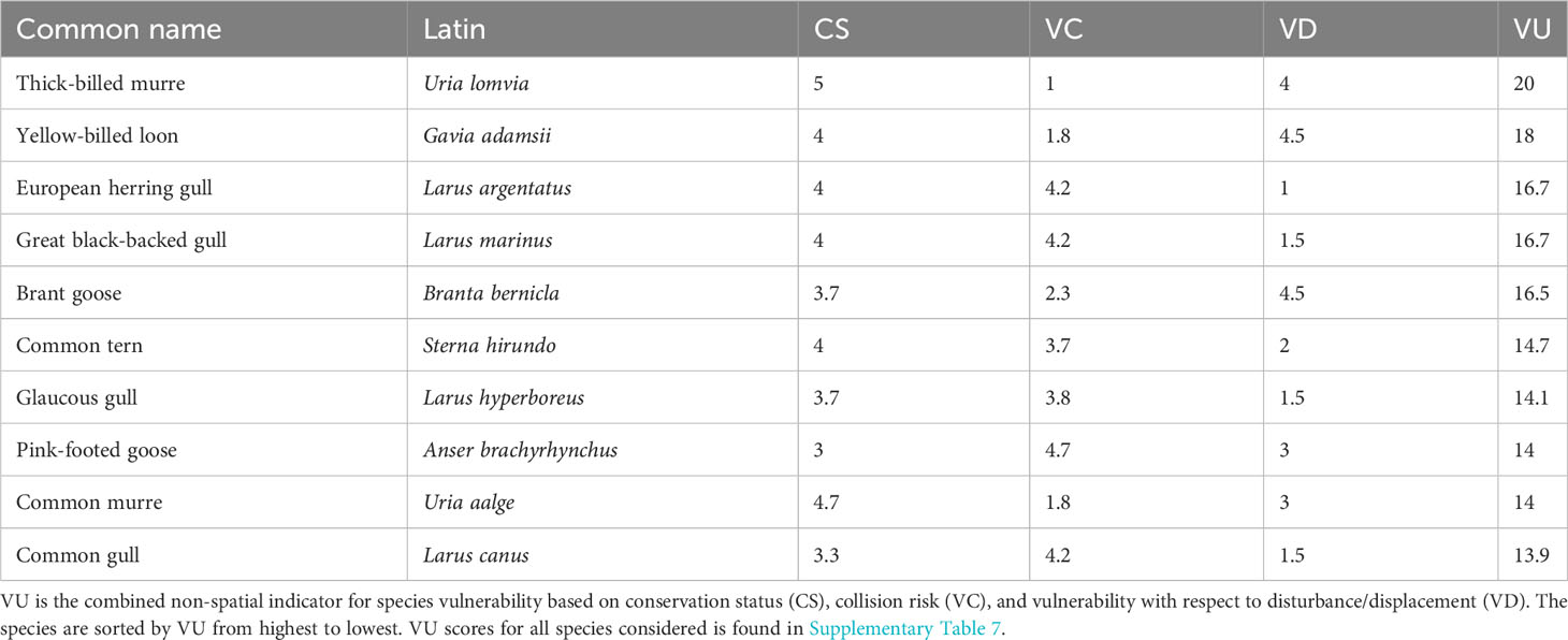
Table 1 The ten species with the highest scores with respect to vulnerability to OWF (VU) in the Norwegian EEZ.

2.4 Vulnerability maps

The species-specific vulnerability scores and maps of habitat suitability were combined to yield a map product consisting of three spatial indicators representing three different levels of detail: (1) Species Vulnerability (SPV) Equation 7 which maps the vulnerability of each species and season, (2) Seasonal Seabird Vulnerability (SSV) Equation 8 which sums the Species Vulnerability in each season, and (3) Total Seabird Vulnerability (TSV) Equation 9 which maps the maximum Seasonal Seabird Vulnerability.

To map the vulnerability of each species and season, predictions from the habitat suitability models were used to distribute the vulnerability in the assessment area. Accordingly, the Species Vulnerability (SPV_i,j,s) in cell i and season j for species s, was defined as the product of habitat suitability (c_i,j,s) and the non-spatial vulnerability indicator (VU_S). Untransformed, the indicator had a skewed distribution with many small values close to zero and few large values. To reduce the skewness of the distribution, the indicator was log_e(x +1) -transformed:

$\begin{array}{ll}SP{V}_{i,j,s}=lo{g}_e(c_{i,j,s}\times V{U}_s+1)& (7)\end{array}$

Seasonal Seabird Vulnerability (SSV_i,j) in cell i and season j was defined as the sum of Species Vulnerability scores for each season and cell:

$\begin{array}{ll}SS{V}_{i,j}={\displaystyle {\sum }_{s}SP{V}_{i,j,s}}& (8)\end{array}$

Finally, Total Seabird Vulnerability (TSV_i) in cell i was defined as the maximum seasonal vulnerability score for each cell:

$\begin{array}{ll}TS{V}_i=\underset{j}{\max }(SS{V}_{i,j})& (9)\end{array}$

2.4.1 Normalization

The spatial vulnerability indicators represent dimensionless values. To give them a relative meaning, the indicators were normalized according to the minimum and maximum indicator values in the assessment area (i.e., (x-min)/(max-min)) and presented as percentages. Accordingly, SPV is expressed as percentage of the maximum SPV value in the assessment area estimated for all species and seasons, SSV is expressed as percentage of the maximum SSV value in the assessment area estimated for all seasons, and TSV is expressed as percentage of the maximum TSV value in the assessment area.

3 Results

Maps of habitat suitability were calculated for 55 species in four seasons (see Supplementary Table 6 for sample sizes and model details). Note that due to seasonal migration in and out of the assessment area, the number of observations were in some cases too few to model habitat suitability. In these cases, habitat suitability was set to zero for the assessment area.

Table 1 shows the non-spatial vulnerability score (VU) together with scores of conservation status (CS), collision risk (VC) and disturbance/displacement (VD) for the ten species with highest VU. In Supplementary Table 7, VU is given for all species considered together with sample statistics of the spatial vulnerability score (SPV) for the assessment area. The table is sorted by VU from high to low vulnerability. Note that the sample statistics of SPV depend on seasonal migration and spatial aggregation. Accordingly, spatially aggregated species with a high VU score had a high maximum SPV and a low mean SPV due to many zeroes.

The importance of the spatiotemporal differences among species is illustrated in Figure 4 which shows maps of SPV for the three species with highest VU score (thick-billed murre, yellow-billed loon Gavia adamsii and herring gull Larus argentatus), and in addition, common tern Sterna hirundo which is a more southern migratory species with a relatively high VU score (Supplementary Table 7). The vulnerability maps reflect differences in spatial distribution and migratory behavior: thick-billed murre and yellow-billed loon are arctic breeding species that migrate north and mainly out of the assessment area during summer. However, while thick-billed murre is a pelagic seabird found over large ocean areas in the Barents Sea, yellow-billed loon is a strictly coastal species wintering in the coastal archipelago in Northern Norway. Herring gulls are found along the entire coast. It has a wide distribution, especially during the non-breeding period when it is frequently observed in offshore shelf areas. Finally, common tern is a coastal migratory species. It breeds along the coast with highest densities in the south and migrates out of the assessment area during winter.

Figure 4

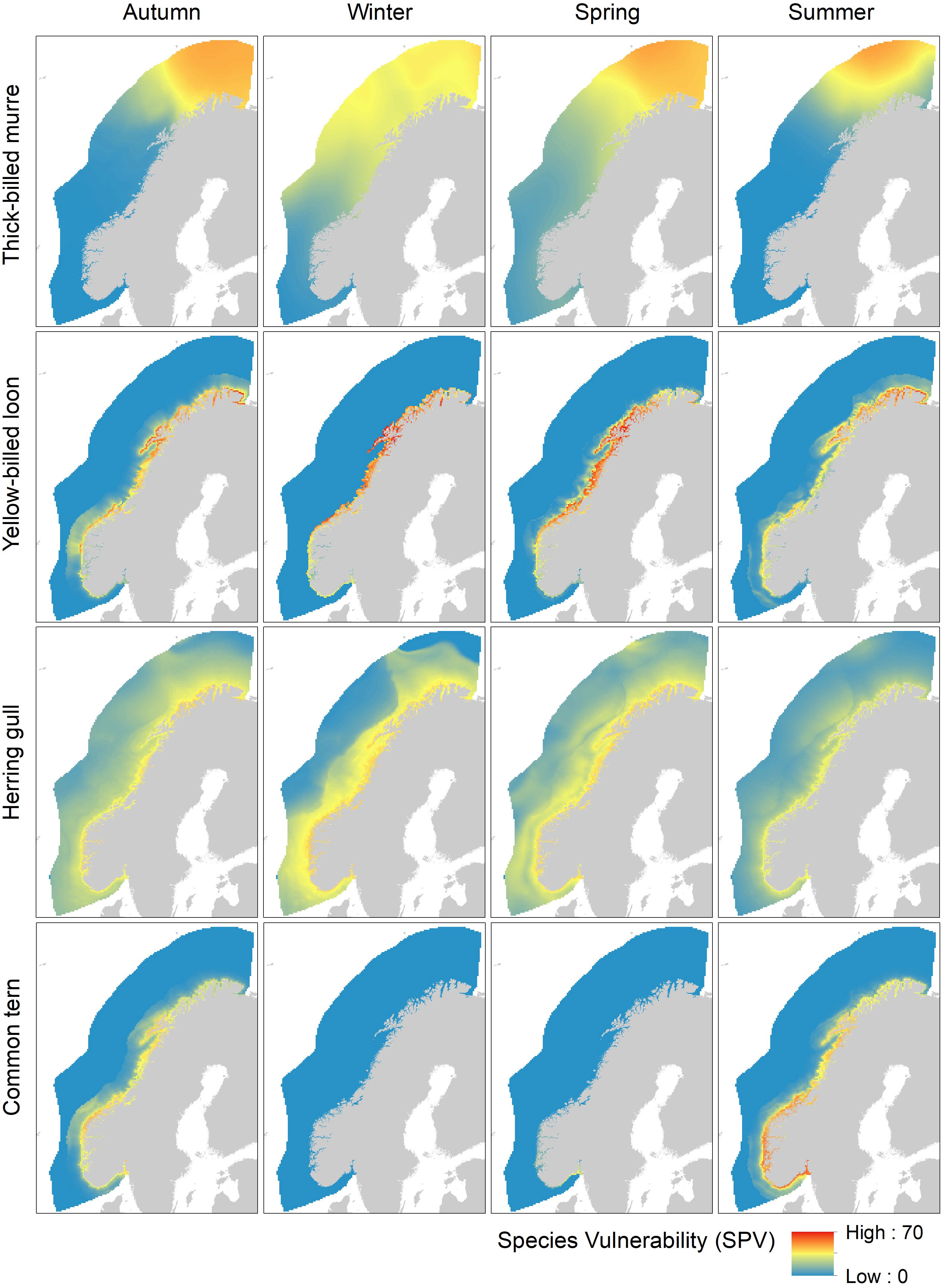
Figure 4 Species vulnerability indicator (SPV) with respect to OWF. The maps show the spatial distribution in SPV scores for four species (thick-billed murre, yellow-billed loon, herring gull and common tern) in four seasons (autumn (August-October), winter (November-January), spring (February-April), and summer (May-July)). SPV is a normalized indicator based on species-specific vulnerability with respect to OWF and habitat suitability.

Summing the species vulnerability scores for all 55 species in each season into the seasonal seabird vulnerability (SSV) indicator, revealed a strong and persistent spatial gradient from high vulnerability along the coast to low vulnerability in offshore areas (Figure 5). To further investigate seasonal differences along the coastal-offshore gradient and differences between ocean areas, we extracted the SSV values for coastal areas (< 100 km from the coastline) and offshore areas (> 100 km from the coastline) for the North Sea, Norwegian Sea, and Barents Sea regions (see definitions in Figure 3). Box-whiskers plots of the distribution of SSV values in different areas and seasons underline the major difference between coastal and offshore areas (Figure 6). Differences between seasons and ocean areas were comparatively small. For the coastal areas (Figure 6A), the three ocean areas had on average similar vulnerability. However, the Barents Sea showed some degree of seasonality with lower values in winter and higher values in summer, suggesting that there was a net migration out of the coastal area during winter. Similar seasonality was not found for the North Sea or the Norwegian Sea. For the offshore areas (Figure 6B), there was an increasing trend in vulnerability from south (North Sea) to north (Barents Sea), suggesting a higher abundance and/or diversity of pelagic seabirds in the north. Seasonality was also more pronounced in the offshore areas and with an increasing trend towards the north.

Figure 5

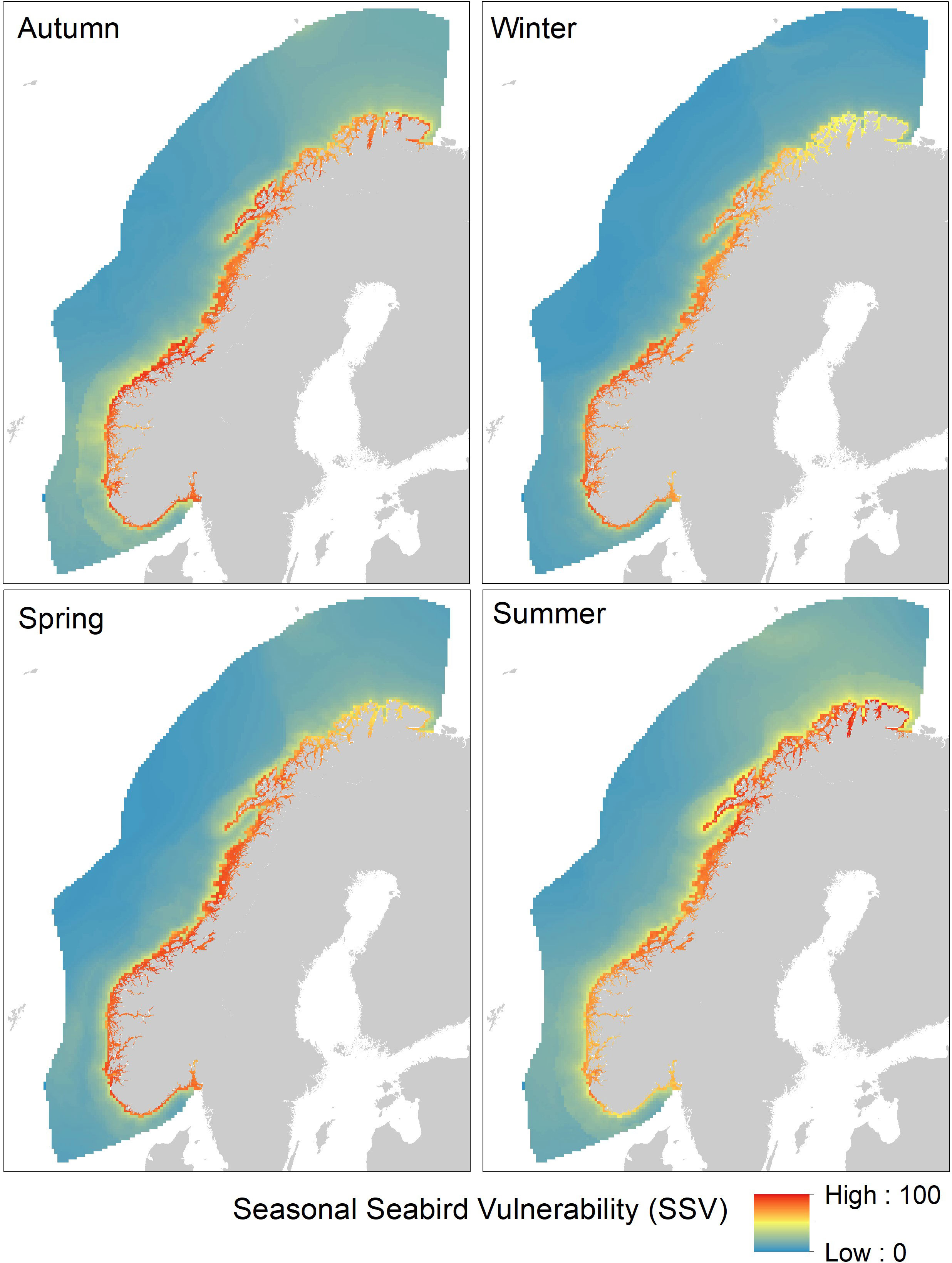
Figure 5 Seasonal Seabird Vulnerability (SSV) with respect to OWF in the Norwegian EEZ. The maps show the spatial distribution of SSV in four seasons (autumn (August-October), winter (November-January), spring (February-April), and summer (May-July)). SSV is the normalized sum of species vulnerability (SPV) from 55 species of seabirds.

Figure 6

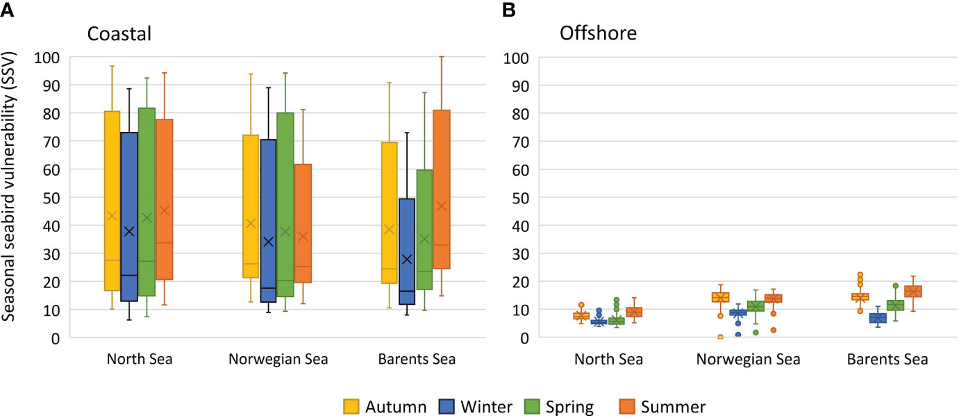
Figure 6 Seasonal seabird vulnerability indicator (SSV). Box-whiskers plot of SSV scores from (A) coastal areas (< 100 km from coastline), and (B) offshore areas (> 100 km from the coastline) in the North Sea, Norwegian Sea and Barents Sea. SSV is the normalized sum of species vulnerability (SPV) from 55 species of seabirds.

The overall seabird vulnerability indicator with respect to OWF (TSV) is shown in Figure 7. Note that this indicator is defined by the normalized maximum seasonal value in each cell. To investigate the dominant inshore-offshore gradient in vulnerability, we plotted the TSV scores as a function of distance from coast (Figure 8). Note the sharp decline in TSV from 0 km (TSV between 68 and 100) to 25 km (TSV between 18 and 39) and a more gradual decline to 50 km (TSV between 14 and 30), 100 km (TSV between 12 and 27), and > 300 km (TSV between 5 and 15).

Figure 7

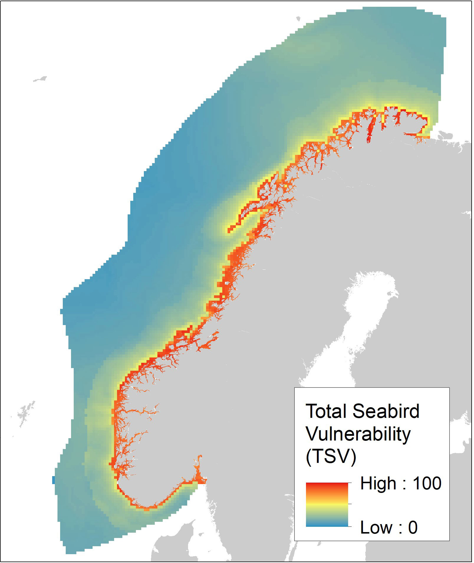
Figure 7 Total Seabird Vulnerability (TSV) with respect to OWF in the Norwegian EEZ. TSV is defined as the normalized maximum seasonal vulnerability and is based on maps of habitat suitability and species-specific vulnerability with respect to OWF for 55 seabird species.

Figure 8

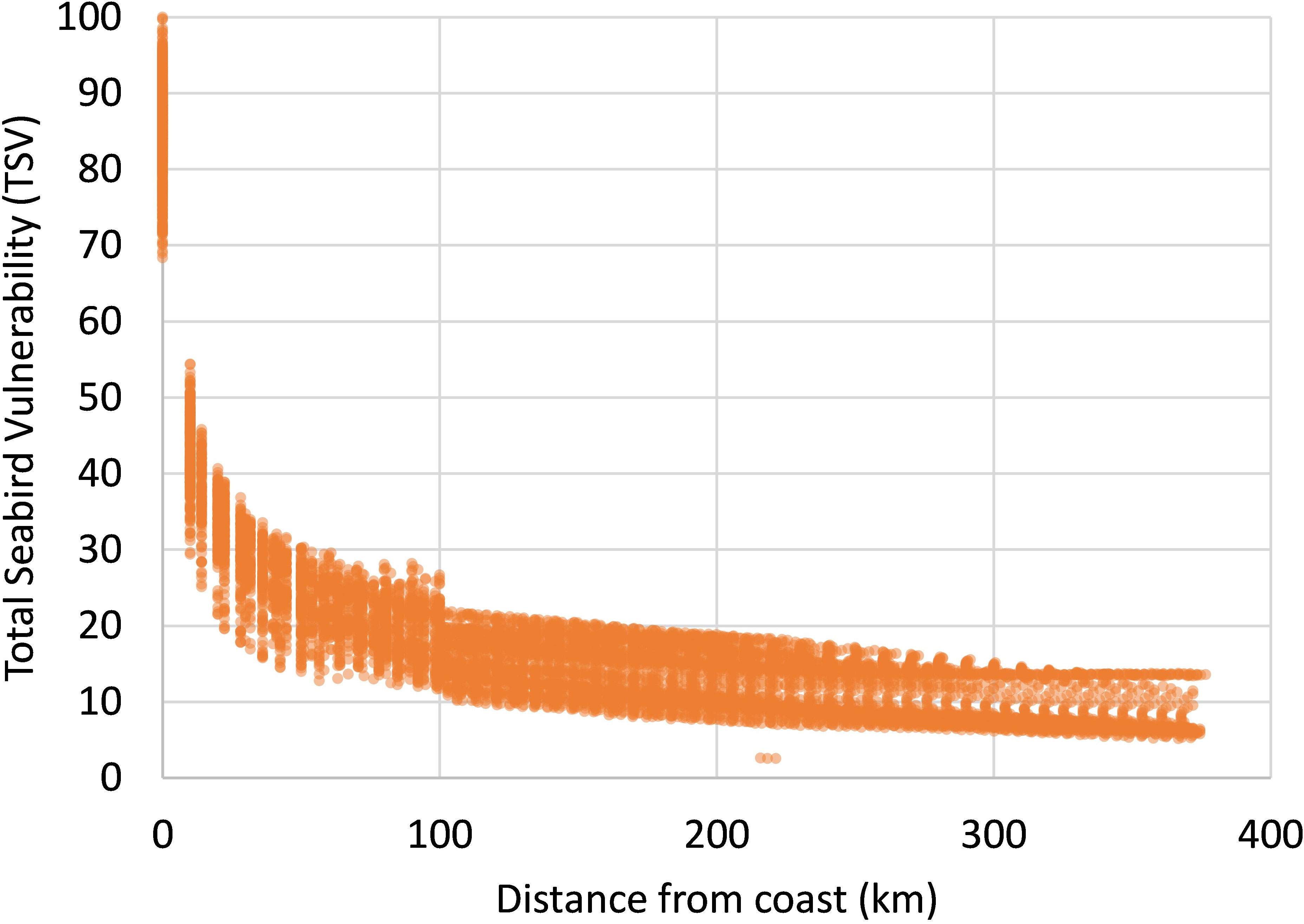
Figure 8 Relationship between Total Seabird Vulnerability (TSV) and distance from coastline. TSV is a normalized indicator based on maps of habitat suitability and species-specific vulnerability with respect to OWF for 55 seabird species.

To illustrate the use of the map product, we extracted the vulnerability scores (total, seasonal and species) for three of the areas proposed for OWED in the Norwegian EEZ (Figure 9). For each area, we calculated the quantiles of total vulnerability (TSV), seasonal vulnerability (SSV), and species vulnerability (SPV). For SPV we show the four species-season combinations with highest average SPV. Note that the most vulnerable species shifted among areas.

Figure 9

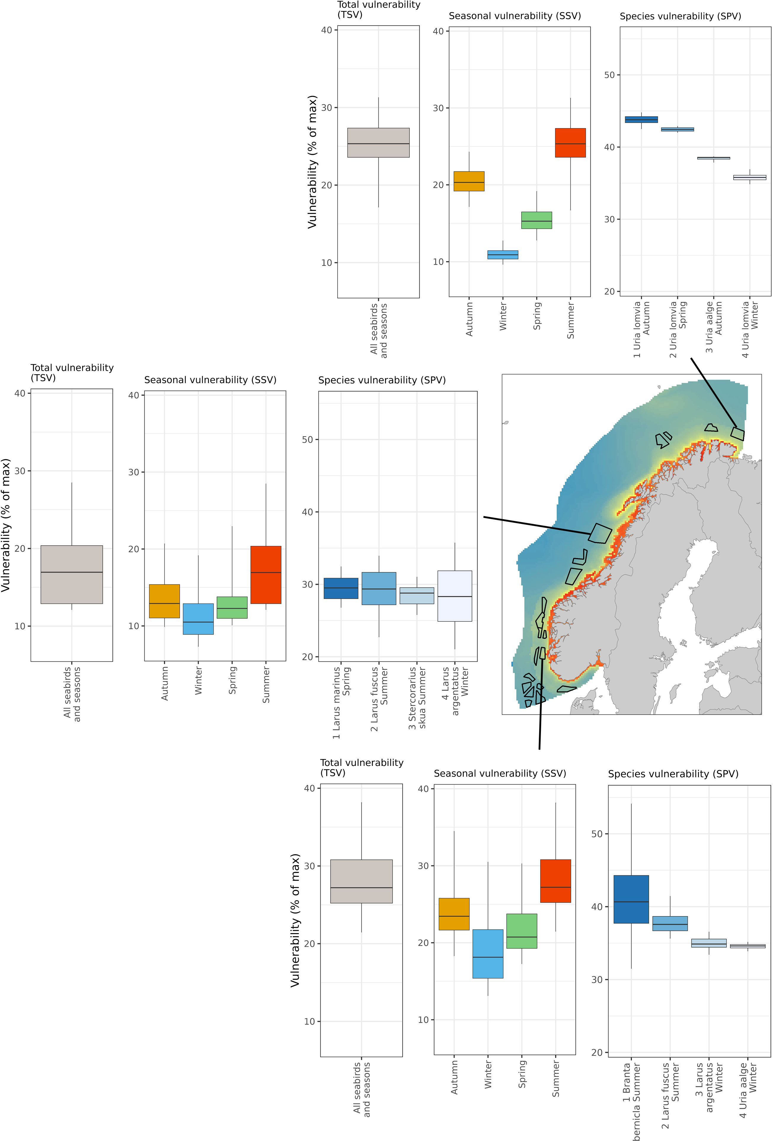
Figure 9 Vulnerability analyses of 3 potential areas for OWED in the Norwegian EEZ. The three map products are illustrated as box-whiskers plots for three identified areas (Nordavind A, Nordvest A and Vestavind F). The left boxplots show the quantiles of total vulnerability scores (TSV) in the proposed areas, the middle boxplots show the quantiles of seasonal vulnerability scores (SSV), and the right boxplots show the quantiles of species vulnerability scores (SPV) for the four most vulnerable species-season combinations. The map shows total seabird vulnerability (TSV) as a color gradient and all the proposed areas for OWED as black polygons.

4 Discussion

By combining species-specific data on vulnerability with habitat suitability maps generated by species distribution models (SDMs), we developed vulnerability maps with respect to offshore wind farms (OWF) for 55 species of marine birds in the Norwegian exclusive economic zone (EEZ). The species included in the analyses represent the most abundant seabirds, marine ducks and geese that occur regularly in Norwegian waters. The maps were summed to yield seasonal maps of seabird vulnerability and a map of the overall vulnerability in the assessment area. The resulting data product targets strategic environmental impact assessments with respect to offshore wind energy development (OWED) in the Norwegian EEZ and represents the currently best available knowledge of the spatial vulnerability of marine birds to OWFs in the assessment area.

Due to differences in seasonal movements of birds within and out of the assessment area, differences in habitat preferences and spatial aggregation, the analyses revealed large variation in spatial vulnerability among species and seasons. However, when summing the spatial vulnerability across species, the combined vulnerability indicator revealed a strong and persistent inshore-offshore gradient from high vulnerability in inshore waters to low vulnerability in offshore waters (Figures 7, 8). Similar inshore-offshore gradients in vulnerability have been found studies carried out in English territorial waters (Bradbury et al., 2014), the US Pacific Outer Continental Shelf (Kelsey et al., 2018), and along the US east coast (Goodale et al., 2019). The inshore-offshore gradient is probably partly related to the restricted activity range away from the breeding locations, and partly a result of a diverse group of coastal species with habitats confined to a narrow strip along the coast. In contrast to the diverse group of coastal species aggregated along the coast, a less diverse pelagic group of seabirds is widely distributed over large ocean areas (Amélineau et al., 2021; Fauchald et al., 2021).

The spatial pattern of the combined vulnerability indicator is probably related to the presence of ecological niches (e.g., Fauchald et al., 2011; Ollus et al., 2023). Different seabird species fill different spatial niches and have different migratory behavior, and if niches are evenly distributed in the habitat, spatial and seasonal variance in vulnerability will decrease as more species are included in the cumulative indicator. However, the interface between terrestrial and marine habitats hosts a myriad of ecological niches for seabirds compared to offshore habitats. Consequently, coastal areas are expected to hold a higher diversity of seabirds and consequently show a higher combined vulnerability across species.

Compared to the inshore-offshore gradient, the differences between ocean areas and seasons were negligible. Interestingly, we found no differences in vulnerability between the coastal areas of the North Sea, Norwegian Sea, and Barents Sea. Accordingly, the indicator does not reflect the geographic distribution of the large seabird colonies which are mainly found in the north (Brun, 1979; Fauchald et al., 2015, Fauchald et al., 2021). However, these colonies are dominated by a few pelagic seabird species (e.g., black-legged kittiwake, common murre and Atlantic puffin), and by summing up the vulnerability of all marine bird species, the spatial difference was cancelled out. The feeding areas around the large seabird cliffs are however highly sensitive areas with respect to OWED as large number of birds commute to and from the colony during summer (Peschko et al., 2020, Peschko et al., 2021). These areas should accordingly be included in the assessment either by incorporating them in the indicator presented here or by a separate assessment.

The data product presented here is particularly relevant in a pre-construction phase where the vulnerability indicators can give input in the siting process of OWFs to avoid or reduce harm to marine birds (Croll et al., 2022). The dominant inshore-offshore gradient found in the present study might suggest that a simple rule of thumb in the siting process is to avoid development in the coastal areas as the harm to seabirds, as quantified by the vulnerability indicator, is expected to be reduced by 70-80% by moving the OWED from the coast to 50-100 km offshore, while little will be gained by moving the project along the coast (Figures 7 and Figure 8). While possibly true, this simplification hides important variation in spatial vulnerability among species (e.g., Figure 9). Indeed, the large variance in habitat use and migration pattern between species revealed in the present study, underlines the importance of incorporating all relevant species in the assessment. The indicator approach, where all available data and knowledge is combined is particularly useful to avoid assessment biases in such large-scale strategic assessments. Moreover, the dataset can be used to identify species and populations of particular concern and thereby guide directed environmental impact assessments as well as mitigation actions and post-constructing monitoring priorities (see Figure 9).

Although the present map product represents the best currently available knowledge, the indicators are associated with complex uncertainties and known, and unknown biases related to the data sampling and the analytical approach (see section 2.2 and 2.3). Importantly, low sampling intensity in remote offshore areas could affect the uncertainty of the SDMs and consequently uncertainty in the predicted habitat suitability. Moreover, the target group approach (Phillips et al., 2009) will generate a higher number of background points in areas with high species diversity and thereby bias the habitat predictions to lower values (Ranc et al., 2017; Vollering et al., 2019). Because coastal waters hold higher seabird diversity, the present predicted inshore-offshore gradient is therefore probably under-estimated. This bias is exacerbated by the log-transformation of the vulnerability scores (eq. 7) which downplay the highly aggregated spatial distribution of coastal species.

The rapid development of offshore wind energy has enabled several recent studies that document the impact of OWF on seabirds through risk of collision (Thaxter et al., 2019; Johnston et al., 2022) and displacement (Mendel et al., 2019; Peschko et al., 2020, Peschko et al., 2021; Garthe et al., 2023). Indeed, the rapid increase in knowledge in this area of research will probably improve the classification and weighing of the vulnerability indicators. OWF is one of many stressors that impact seabirds in the marine environment (Croxall et al., 2012; Dias et al., 2019) and incorporating other human stressors in the indicators could be an important addition to the present approach. Finally, climate change and other anthropogenic impacts are currently changing marine ecosystems and consequently the distribution and abundance of seabirds (Cooley et al., 2022). In sum, improved data, knowledge and statistical methods combined with a changing marine environment suggest that the relevance of the data product presented here has a limited time horizon and should be updated regularly.

Data availability statement

Publicly available datasets were analyzed in this study. This data can be found here: Links to the datasets are provided in the text. The data and code supporting the conclusions of this article will be made available by the corresponding author, without undue reservation.

Author contributions

PF: Conceptualization, Data curation, Formal analysis, Methodology, Validation, Writing – original draft, Writing – review & editing. VO: Conceptualization, Data curation, Formal analysis, Methodology, Writing – original draft, Writing – review & editing. MB: Data curation, Formal analysis, Writing – review & editing. AB: Data curation, Validation, Writing – review & editing. SC-D: Conceptualization, Data curation, Methodology, Writing – review & editing. SM: Data curation, Validation, Writing – review & editing. AT: Methodology, Validation, Writing – review & editing. GS: Data curation, Methodology, Writing – review & editing. BM: Conceptualization, Data curation, Methodology, Project administration, Writing – review & editing.

Funding

The author(s) declare financial support was received for the research, authorship, and/or publication of this article. This research was funded by The Norwegian Water Resources and Energy Directorate (NVE), and the seabird monitoring programs SEATRACK and SEAPOP.

Acknowledgments

The authors thank Dr. Svein-Håkon Lorentsen and Jørund Braa for guidance and support during the study.

Conflict of interest

The authors declare that the research was conducted in the absence of any commercial or financial relationships that could be construed as a potential conflict of interest.

Publisher’s note

All claims expressed in this article are solely those of the authors and do not necessarily represent those of their affiliated organizations, or those of the publisher, the editors and the reviewers. Any product that may be evaluated in this article, or claim that may be made by its manufacturer, is not guaranteed or endorsed by the publisher.

Supplementary material

The Supplementary Material for this article can be found online at: https://www.frontiersin.org/articles/10.3389/fmars.2024.1335224/full#supplementary-material

References

Amante C., Eakins B. W. (2009). ETOPO1 1 Arc-Minute Global Relief Model: Procedures, Data Sources and Analysis. (National Geophysical Data Center, NOAA: NOAA Technical Memorandum NESDIS NGDC-24). doi: 10.7289/V5C8276M

CrossRef Full Text | Google Scholar

Amélineau F., Merkel B., Tarroux A., Descamps S., Anker-Nilssen T., Bjørnstad O., et al. (2021). Six pelagic seabird species of the North Atlantic engage in a fly-and-forage strategy during their migratory movements. Mar. Ecol. Prog. Ser. 676, 127–144. doi: 10.3354/meps13872

CrossRef Full Text | Google Scholar

Artsdatabanken (2022). Norwegian redlist for species 2021. Available at: https://artsdatabanken.no/lister/rodlisteforarter/2021/.

Google Scholar

Artsobs (2023) Artsobservasjoner. Available online at: https://www.artsobservasjoner.no/.

Google Scholar

Barber R. A., Ball S. G., Morris R. K. A., Gilbert F. (2022). Target-group backgrounds prove effective at correcting sampling bias in Maxent models. Divers. Distrib. 28, 128–141. doi: 10.1111/ddi.13442

CrossRef Full Text | Google Scholar

BirdLife International (2021). European Red List of Birds (Luxembourg: Publications Office of the European Union).

Google Scholar

Bradbury G., Trinder M., Furness B., Banks A. N., Caldow R. W. G., Hume D. (2014). Mapping Seabird Sensitivity to offshore wind farms. PLoS One 9, e106366. doi: 10.1371/journal.pone.0106366

PubMed Abstract | CrossRef Full Text | Google Scholar

Brun E. (1979). “Present status and trends of seabirds in Norway,” in Conervation of Marine Birds of Northern North America. Eds. Bartonek J. C., Nettleship D. N. (U.S. Fish and Wildlife Service: Seattle, Washington).

Google Scholar

Cleasby I. R., Owen E., Wilson L., Wakefield E. D., O’Connell P., Bolton M. (2020). Identifying important at-sea areas for seabirds using species distribution models and hotspot mapping. Biol. Conserv. 241, 108375. doi: 10.1016/j.biocon.2019.108375

CrossRef Full Text | Google Scholar

Cooley S., Schoeman D., Bopp L., Boyd P., Donner S., Ghebrehiwet D. Y., et al. (2022). Oceans and Coastal Ecosystems and Their Services. In Climate Change 2022: Impacts, Adaptation and Vulnerability. Ed. Pörtner H. -O., Roberts D. C., Tignor M., Poloczanska E. S., Mintenbeckr K., Alegría A., et al. UK and New York, NY, USA: Cambridge University Press. 379–550. doi: 10.1017/9781009325844.005

CrossRef Full Text | Google Scholar

Croll D. A., Ellis A. A., Adams J., Cook A. S. C. P., Garthe S., Goodale M. W., et al. (2022). Framework for assessing and mitigating the impacts of offshore wind energy development on marine birds. Biol. Conserv. 276, 109795. doi: 10.1016/j.biocon.2022.109795

CrossRef Full Text | Google Scholar

Croxall J. P., Butchart S. H. M., Lascelles B., Stattersfield A. J., Sullivan B., Symes A., et al. (2012). Seabird conservation status, threats and priority actions: A global assessment. Bird Conserv. Int. 22, 1–34. doi: 10.1017/S0959270912000020

CrossRef Full Text | Google Scholar

Dias M. P., Martin R., Pearmain E. J., Burfield I. J., Small C., Phillips R. A., et al. (2019). Threats to seabirds: A global assessment. Biol. Conserv. 237, 525–537. doi: 10.1016/j.biocon.2019.06.033

CrossRef Full Text | Google Scholar

Dierschke V., Furness R. W., Garthe S. (2016). Seabirds and offshore wind farms in European waters: Avoidance and attraction. Biol. Conserv. 202, 59–68. doi: 10.1016/j.biocon.2016.08.016

CrossRef Full Text | Google Scholar

Elith J., Leathwick J. R. (2009). Species distribution models: Ecological explanation and prediction across space and time. Annu. Rev. Ecol. Evol. Syst. 40, 677–697. doi: 10.1146/annurev.ecolsys.110308.120159

CrossRef Full Text | Google Scholar

ESAS (2022). European Seabirds At Sea (ESAS) (Copenhagen, Denmark: ICES). Available at: https://esas.ices.dk.

Google Scholar

Fauchald P. (2011). Sjøfugl i åpent hav. Utbredelsen av sjøfugl i norske og tilgrensende havområder. NINA Rapport, 786.

Google Scholar

Fauchald P., Anker-Nilssen T., Barrett R. T., Bustnes J. O., Bårdsen B., Christensen-Dalsgaard S., et al. (2015). The status and trends of seabirds breeding in Norway and Svalbard. NINA Rep., 1151.

Google Scholar

Fauchald P., Skov H., Skern-Mauritzen M., Hausner V. H., Johns D., Tveraa T. (2011). Scale-dependent response diversity of seabirds to prey in the North Sea. Ecology 92, 228–239. doi: 10.1890/10-0818.1

PubMed Abstract | CrossRef Full Text | Google Scholar

Fauchald P., Tarroux A., Amélineau F., Bråthen V. S., Descamps S., Ekker M., et al. (2021). Year-round distribution of Northeast Atlantic seabird populations: Applications for population management and marine spatial planning. Mar. Ecol. Prog. Ser. 676, 255–276. doi: 10.3354/meps13854

CrossRef Full Text | Google Scholar

Furness R. W., Wade H. M., Masden E. A. (2013). Assessing vulnerability of marine bird populations to offshore wind farms. J. Environ. Manage. 119, 56–66. doi: 10.1016/j.jenvman.2013.01.025

PubMed Abstract | CrossRef Full Text | Google Scholar

Garthe S., Hüppop O. (2004). Scaling possible adverse effects of marine wind farms on seabirds: Developing and applying a vulnerability index. J. Appl. Ecol. 41, 724–734. doi: 10.1111/j.0021-8901.2004.00918.x

CrossRef Full Text | Google Scholar

Garthe S., Schwemmer H., Peschko V., Markones N., Müller S., Schwemmer P., et al. (2023). Large-scale effects of offshore wind farms on seabirds of high conservation concern. Sci. Rep. 13, 4779. doi: 10.1038/s41598-023-31601-z

PubMed Abstract | CrossRef Full Text | Google Scholar

Goodale M. W., Milman A., Griffin C. R. (2019). Assessing the cumulative adverse effects of offshore wind energy development on seabird foraging guilds along the East Coast of the United States. Environ. Res. Lett. 14, 074018. doi: 10.1088/1748-9326/ab205b

CrossRef Full Text | Google Scholar

Halpern B. S., Fujita R. (2013). Assumptions, challenges, and future directions in cumulative impact analysis. Ecosphere 4, 1–11. doi: 10.1890/ES13-00181.1

CrossRef Full Text | Google Scholar

Halpern B. S., Longo C., Hardy D., McLeod K. L., Samhouri J. F., Katona S. K., et al. (2012). An index to assess the health and benefits of the global ocean. Nature 488, 615–620. doi: 10.1038/nature11397

PubMed Abstract | CrossRef Full Text | Google Scholar

Halpern B. S., Walbridge S., Selkoe K., Kappel C. V., Micheli F., D’Agrosa C., et al. (2008). A global map of human impact on marine ecosystems. Science 319, 948–952. doi: 10.1126/science.1149345

PubMed Abstract | CrossRef Full Text | Google Scholar

Hijmans R. J. (2023) terra: Spatial Data Analysis. R package version 1.7-39. Available online at: https://cran.r-project.org/package=terra.

Google Scholar

Huang B., Liu C., Banzon V., Freeman E., Graham G., Hankins B., et al. (2021). Improvements of the daily optimum interpolation sea surface temperature (DOISST) version 2.1. J. Clim. 34, 2923–2939. doi: 10.1175/JCLI-D-20-0166.1

CrossRef Full Text | Google Scholar

ICES Data Portal (2022). Dataset on Ocean Hydrochemistry (Copenhagen: ICES). Available at: www.ices.dk/data/dataset-collections.

Google Scholar

Issaris Y., Katsanevakis S., Pantazi M., Vassilopoulou V., Panayotidis P., Kavadas S., et al. (2012). Ecological mapping and data quality assessment for the needs of ecosystem-based marine spatial management: Case study Greek Ionian Sea and the adjacent gulfs. Mediterr. Mar. Sci. 13, 297–311. doi: 10.12681/mms.312

CrossRef Full Text | Google Scholar

Johnston D. T., Thaxter C. B., Boersch-Supan P. H., Humphreys E. M., Bouten W., Clewley G. D., et al. (2022). Investigating avoidance and attraction responses in lesser black-backed gulls Larus fuscus to offshore wind farms. Mar. Ecol. Prog. Ser. 686, 187–200. doi: 10.3354/meps13964

CrossRef Full Text | Google Scholar

Kelsey E. C., Felis J. J., Czapanskiy M., Pereksta D. M., Adams J. (2018). Collision and displacement vulnerability to offshore wind energy infrastructure among marine birds of the Pacific Outer Continental Shelf. J. Environ. Manage. 227, 229–247. doi: 10.1016/j.jenvman.2018.08.051

PubMed Abstract | CrossRef Full Text | Google Scholar

King S., Maclean I. M. D., Norman T., Prior A. (2009). Developing guidance on ornithological cumulative impact assessment for offshore wind farm developers. COWRIE. 1–41.

Google Scholar

Legendre P., Legendre L. (2012). Numerical Ecology. 3rd ed (Elsevier Science: Amsterdam, The Netherlands).

Google Scholar

May R., Jackson C. R., Middel H., Stokke B. G., Verones F. (2021). Life-cycle impacts of wind energy development on bird diversity in Norway. Environ. Impact Assess. Rev. 90. doi: 10.1016/j.eiar.2021.106635

PubMed Abstract | CrossRef Full Text | Google Scholar

May R., Middel H., Stokke B. G., Jackson C., Verones F. (2020). Global life-cycle impacts of onshore wind-power plants on bird richness. Environ. Sustain. Indic. 8. doi: 10.1016/j.indic.2020.100080

CrossRef Full Text | Google Scholar

Mendel B., Schwemmer P., Peschko V., Müller S., Schwemmer H., Mercker M., et al. (2019). Operational offshore wind farms and associated ship traffic cause profound changes in distribution patterns of Loons (Gavia spp.). J. Environ. Manage. 231, 429–438. doi: 10.1016/j.jenvman.2018.10.053

PubMed Abstract | CrossRef Full Text | Google Scholar

Norberg A., Abrego N., Blanchet F. G., Adler F. R., Anderson B. J., Anttila J., et al. (2019). A comprehensive evaluation of predictive performance of 33 species distribution models at species and community levels. Ecol. Monogr. 89, 1370. doi: 10.1002/ecm.1370

CrossRef Full Text | Google Scholar

NVE (2023) Identifisering av utredningsområder for havvind. Available online at: https://veiledere.nve.no/havvind/identifisering-av-utredningsomrader-for-havvind/.

Google Scholar

Ollus V. M. S., Biuw M., Lowther A., Fauchald P., Deehr Johannessen J. E., Martín López L. M., et al. (2023). Large-scale seabird community structure along oceanographic gradients in the Scotia Sea and northern Antarctic Peninsula. Front. Mar. Sci. 10. doi: 10.3389/fmars.2023.1233820

CrossRef Full Text | Google Scholar

Perrow M. R. (2019). Wildlife and Wind Farms - Conflicts and Solutions. Volume 3 Offshore: Potential Effects (Exeter, UK: Pelagic Publishing).

Google Scholar

Peschko V., Mendel B., Mercker M., Dierschke J., Garthe S. (2021). Northern gannets (Morus bassanus) are strongly affected by operating offshore wind farms during the breeding season. J. Environ. Manage. 279, 111509. doi: 10.1016/j.jenvman.2020.111509

PubMed Abstract | CrossRef Full Text | Google Scholar

Peschko V., Mendel B., Müller S., Markones N., Mercker M., Garthe S. (2020). Effects of offshore windfarms on seabird abundance: Strong effects in spring and in the breeding season. Mar. Environ. Res. 162, 105157. doi: 10.1016/j.marenvres.2020.105157

PubMed Abstract | CrossRef Full Text | Google Scholar

Phillips S. J., Dudík M., Elith J., Graham C. H., Lehmann A., Leathwick J., et al. (2009). Sample selection bias and presence-only distribution models: Implications for background and pseudo-absence data. Ecol. Appl. 19, 181–197. doi: 10.1890/07-2153.1

PubMed Abstract | CrossRef Full Text | Google Scholar

Ranc N., Santini L., Rondinini C., Boitani L., Poitevin F., Angerbjörn A., et al. (2017). Performance tradeoffs in target-group bias correction for species distribution models. Ecography (Cop.). 40, 1076–1087. doi: 10.1111/ecog.02414

CrossRef Full Text | Google Scholar

R Core Team. (2023). R: A Language and Environment for Statistical Computing. R Foundation for Statistical Computing: Vienna, Austria. Available at: https://www.R-project.org/.

Google Scholar

Robinson Willmott J. C., Forcey G., Kent A. (2013). The relative vulnerability of migratory bird species to offshore wind energy projects on the atlantic outer continental shelf: An assessment method and database. Final report to the U.S. Department of the interior, bureau of ocean energy management. OCS Study BOEM 2013–207, 1:275.

Google Scholar

SEAPOP (2023) SEAPOP. Available online at: https://seapop.no/en/.

Google Scholar

SEATRACK (2023) SEATRACK. Available online at: https://seapop.no/en/seatrack/.

Google Scholar

Tasker M. L., Hope Jones O., Dixon T. I. M., Blake B. F., Jones P. H. (1984). Counting seabirds from ships: a review of methods employed and a suggestion for a standardized approach. Auk 101, 567–577. doi: 10.1093/auk/101.3.567

CrossRef Full Text | Google Scholar

Thaxter C. B., Ross-Smith V. H., Bouten W., Clark N. A., Conway G. J., Masden E. A., et al. (2019). Avian vulnerability to wind farm collision through the year: Insights from lesser black-backed gulls (Larus fuscus) tracked from multiple breeding colonies. J. Appl. Ecol. 56, 2410–2422. doi: 10.1111/1365-2664.13488

CrossRef Full Text | Google Scholar

Vanermen N., Onkelinx T., Courtens W., Van de walle M., Verstraete H., Stienen E. W. M. (2015). Seabird avoidance and attraction at an offshore wind farm in the Belgian part of the North Sea. Hydrobiologia 756, 51–61. doi: 10.1007/s10750-014-2088-x

CrossRef Full Text | Google Scholar

Vollering J., Halvorsen R., Auestad I., Rydgren K. (2019). Bunching up the background betters bias in species distribution models. Ecography (Cop.). 42, 1717–1727. doi: 10.1111/ecog.04503

CrossRef Full Text | Google Scholar

Wood S. N. (2017). ). Generalized additive models: An introduction with R, second edition. Chapman and Hall/CRC: Boca Raton, US. doi: 10.1201/9781315370279

CrossRef Full Text | Google Scholar