DWSTr: a hybrid framework for ship-radiated noise recognition

The critical nature of passive ship-radiated noise recognition for military and economic security is well-established, yet its advancement faces significant obstacles due to the complex marine environment. The challenges include natural sound interference and signal distortion, complicating the extraction of key acoustic features and ship type identification. Addressing these issues, this study introduces DWSTr, a novel method combining a depthwise separable convolutional neural network with a Transformer architecture. This approach effectively isolates local acoustic features and captures global dependencies, enhancing robustness against environmental interferences and signal variability. Validated by experimental results on the ShipsEar dataset, DWSTr demonstrated a notable 96.5\% recognition accuracy, underscoring its efficacy in accurate ship classification amidst challenging conditions. The integration of these advanced neural architectures not only surmounts existing barriers in noise recognition but also offers computational efficiency for real-time analysis, marking a significant advancement in passive acoustic monitoring and its application in strategic and economic contexts.

1 Introduction

Ship-radiated noise plays a critical role as a significant source of oceanic noise, making its recognition essential across diverse domains, including maritime security, navigation, environmental monitoring, and ocean research. However, the recognition of ship-radiated noise in the real marine environment poses significant challenges. The underwater environment comprises various types of underwater acoustic signals resulting from ocean movements, marine creatures, vessels, etc. The unwanted presence of natural sounds can greatly obscure the target’s signals, posing a great challenge to accurately identify and discern the distinct features of ship-radiated noises.

In addition to the interference caused by ambient noise, the challenge of accurately identifying ship targets based on their radiated noises is intensified by the inevitable attenuation and distortion that occur in received acoustic signals. Furthermore, the noise emitted by a ship is primarily attributed to the vibrations generated by its various components. These vibrations result in a multifaceted soundscape consisting of mechanical noise, propeller noise, hydrodynamic noise, and other contributing factors (Li and Yang, 2021). The intricate blend of these auditory elements poses a significant challenge that makes it difficult to solely rely on the analysis of radiated noise to accurately identify ship targets.

In the field of recognition tasks, researchers primarily focus on two crucial aspects: feature extraction and classifier design. The process of feature extraction involves extracting meaningful and relevant information from the input data and transforming it into a more compact and representative format. On the other hand, classifier design involves the creation and implementation of models that can effectively classify and categorize the extracted features.

In the field of feature extraction methods, the traditional approaches such as the discrete wavelet transform (DWT) (Mallat, 1989), the low-frequency array (LOFAR) (Polatidis et al., 2013), and the detection of envelope modulation on noise (DEMON) (Pollara et al., 2016) are valuable in certain applications, but they may struggle to address the full range of challenges posed by underwater acoustic signals.

The DWT, which decomposes signals into different frequency bands, faces challenges in differentiating desired signals from background noise and environmental interference, as highlighted in academic literature. Key disadvantages identified include shift sensitivity, where DWT’s output can vary significantly with slight input shifts, limiting its use in precise signal localization; poor directionality, which restricts its effectiveness in multidimensional signal processing, like image analysis; and the inability to preserve phase information, crucial for detailed signal structure and timing (Fernandes et al., 2004). Furthermore, the computational complexity and resource consumption of conventional DWT, as discussed by Alzaq et al. (Alzaq and Üstündağ, 2018) present further challenges, particularly in areas requiring low-frequency focus.

LOFAR spectra transform signals from the time domain to the time-frequency domain using shorttime Fourier transform (STFT), which is particularly significant for sound source information with a high signal-to-noise ratio. As discussed by Chen et al. (Chen et al., 2021) and Luo et al. (Luo and Feng, 2020), the process implies that LOFAR is more attuned to identifying low-frequency elements in sonar ship target recognition, which may suggest inherent limitations in capturing high-frequency details.

DEMON, a technique for monitoring and detecting impulsive underwater sounds, faces challenges in real-time analysis and adaptability to changing noise conditions, as discussed by Tian et al. (Tian et al., 2023). Its effectiveness in recognizing different types of underwater acoustic events or sources is limited, especially when dealing with complex and variable noise signatures.

Auditory-characteristic-based extraction methods, such as Mel-frequency cepstral coefficients (MFCCs) (Davis and Mermelstein, 1980a) and Mel-spectrogram (Davis and Mermelstein, 1980b), can help mitigate the shortcomings mentioned above (Hinton et al., 2012). By mapping the signal’s frequency content to the mel-scale, these methods provide improved frequency resolution, enabling the capture of nuances in underwater acoustic signals. Additionally, they exhibit noise robustness through logarithmic compression, which emphasizes perceptually relevant features while suppressing noise components. Thus the performance is enhanced in the presence of additive noise. However, the inclusion of the Discrete Cosine Transform (DCT) in MFCCs can inadvertently filter out valuable information and increase computational complexity. However, Mel-spectrograms can directly represent the signal’s complete spectral information, including both magnitude and phase, without requiring additional computation steps or omitting crucial details. Therefore, in this paper, the choice of feature extraction method to handle raw underwater acoustic data falls on the Mel-spectrogram.

Previous studies have demonstrated the application of statistical classifiers in the field of underwater acoustic signal recognition, showcasing notable achievements (Filho et al., 2011; Yang et al., 2016; Tong et al., 2020). However, achieving promising results often requires sophisticated feature engineering and abundant prior knowledge. Furthermore, the statistical approaches usually entail a relatively complex process of partitioning the problem into multiple subsections and then accumulating the results (Khishe, 2022).

Deep learning methods provide effective solutions to handle the limitations mentioned above, which have brought new ideas to strengthen data analysis and improve the accuracy of shipradiated noise recognition. Their automatic feature extraction capability eliminates the need for manual engineering. However, there are inherent deficiencies in traditional network architectures like Deep Belief Networks (DBNs) (Zhao et al., 2016; Tang et al., 2017; Yang et al., 2018; Wu et al., 2019)and Convolutional Neural Networks (CNNs) (Chen et al., 2017; Wang et al., 2017; Chen et al., 2018; Shen et al., 2018). While excelling in capturing local features and preserving locality, they struggle with comprehending long-range dependencies and capturing global temporal patterns. Designed primarily for local feature extraction, they lack effectiveness in capturing broader temporal relationships within ship-radiated noise data. Additionally, their inherent computing mechanisms make them computationally expensive and time-consuming.

Perotin et al. (Perotin et al., 2019) introduce a method that combines CNN blocks with a recurrent neural network (RNN) block to enhance classification accuracy by capturing temporal dependencies, where CNN blocks extract locally invariant high-level features and the RNN block gathers related features. However, the use of RNN introduces the short-term memory problem, hindering the network’s ability to learn long-term dependencies. For longer input sequences, the RNN model may neglect information at the beginning (Zhou et al., 2018). Although CNNs can partially address this issue by applying different kernels to the input sequence, as the maximum length of the input sequence increases, the number of kernels required to capture dependencies grows exponentially. This can result in ineffective training and model overfitting, limiting the model’s performance. Therefore, there is a need for alternative approaches that can address long-term dependencies more effectively while avoiding potential training and overfitting challenges caused by an increasing number of parameters.

The Transformer was initially introduced in natural language processing (Vaswani et al., 2017; Devlin et al., 2018; Brown et al., 2020) to overcome recursion and enable parallel computations, reducing training time and minimizing performance drops due to long dependencies. Being a non-sequential model that doesn’t rely on past hidden states, the Transformer exhibits robust global computation and flawless memory, making it more suitable for processing lengthy sequences compared to RNNs. In the domain of ship-radiated noise signal recognition, the Transformer architecture has emerged as a pivotal tool, adeptly handling complex acoustic signals. Li et al. (Li et al., 2023) demonstrated the Transformer’s proficiency in learning temporal information under low signal-to-noise ratios, significantly bolstering signal recognition and denoising. Feng et al. (Feng and Zhu, 2022) delved into the Transformer’s core feature, the attention mechanism, highlighting its effectiveness in isolating critical signal features amidst substantial background interference. Yang et al. (Yang et al., 2023) innovatively merged two-dimensional adaptive compact variational mode decomposition with the Transformer, enhancing the extraction and denoising of ship-radiated noise textures, thereby markedly surpassing traditional methodologies. This transformative approach in underwater acoustic signal processing stands as a beacon, offering a robust solution to the complexities inherent in marine environments.

The rising trend of researchers proposing transformer-based models to improve various tasks highlights the growing interest in their capabilities. However, it is important to note that the Transformer stands out with its notably reduced spatial-specific inductive bias compared to CNNs (Dosovitskiy et al., 2020). This distinction arises from inherently integrating locality, twodimensional neighborhood structure, and translation equivariance across all layers for CNNs. Jin et al. (Jin and Zeng, 2023) adeptly combine the Res-Dense CNN with the Transformer’s attention mechanism to address ship-radiated noise challenges in complex marine environments. They leverage the Residuals CNN module to prevent network degradation, while the attention mechanism effectively highlights important features in time series data. Duan et al. (Duan et al., 2022) employ signal enhancement techniques alongside a one-dimensional CNN and Vision Transformer’s multihued attention mechanism. This innovative approach significantly boosts the signal-to-noise ratio of ship-radiated noise, particularly in extremely low signal-to-noise conditions ranging from -20 dB to -25 dB.

In the complex marine environment, ship sound recordings are often contaminated by persistent, irregular background noise. To develop an effective recognition model, it is crucial to denoise the data while preserving the essential feature dependencies present in the original recordings. This study takes inspiration from the CRNN architecture and proposes a novel approach that combines a depthwise separable convolutional neural network (DWSCNN) with a Transformer. This integration aims to enhance the model’s ability to capture both spatial characteristics and feature dependencies accurately. By decomposing the convolution operation into separate depthwise and pointwise stages, the computational complexity can be significantly reduced. This reduction in complexity makes the DWSCNN more efficient than traditional CNNs, particularly when operating on large-scale datasets or in resource-constrained environments.

The contributions in this paper can be summarized as:

1. In order to address the performance degradation resulting from long-term dependencies and noisy input data, we introduce a Transformer approach. The model can automatically assign higher importance to relevant information frames, thereby enabling improved modeling of spectral dependencies and capturing critical temporal dependencies.

2. In order to enhance spatial modeling in underwater acoustic signal recognition, we propose a DWSCNN combined with the Transformer framework. The model gains the ability to effectively analyze and interpret spatial characteristics, leading to more precise and reliable results in recognizing underwater acoustic signals.

3. In order to reduce computational complexity and realize real-time analysis, the convolution operation is separated into pointwise and depthwise stages. This separation allows for more efficient processing, reducing the overall computational load and enabling faster analysis of data.

The rest of the paper is structured as follows. Section II details the methodology of feature extraction and the proposed neural network. Section III presents the dataset used in this paper and analyses conducted from experimental results. Finally, conclusions are given in section IV.

2 Methodology

2.1 System overview

This paper proposes a hybrid network, DWSTr, to ensure data integrity and model efficiency. The spectrogram is initially processed by the DWS block, generating a two-dimensional spatial feature mapping. This mapping is then flattened, segmented, and position-embedded, forming a one-dimensional sequence. The Transformer block subsequently processes the entire sequence, learning the timing correlation information. By combining the strengths of the DWS block and Transformer block, the proposed network effectively maintains the integrity of the data while efficiently capturing timing correlations, leading to improved performance. The overall architecture of the proposed model is shown in Figure 1.

Figure 1

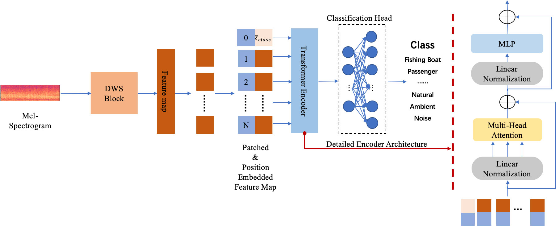
Figure 1 The overall architecture of the proposed method in this paper: (1) the audio signal’s Mel-spectrogram is used as the input; (2) a DWS block is employed to extract spatial features and the generated feature map is used as the Transformer’s input; (3) a Transformer is adopted to automatic learn temporal features and classify the target.

2.2 Feature extraction

In the dataset, each recorded ship-radiated noise sample is stored as a one-dimensional array based on the audio length and sampling rate. Extracting informative feature representations necessitates the use of Mel-spectrograms since they offer a distinct advantage due to their ability to comprehensively represent the raw data while also providing flexibility in parameter selection, such as window length and overlap. This adaptability allows for customization that aligns with the specific requirements of underwater acoustic analysis. Moreover, Mel-spectrograms seamlessly integrate into deep learning models because they can directly process spectrogram-like inputs. Hence, they are exceptionally well-suited for acoustic signal recognition tasks that involve the utilization of neural networks. Figure 2 shows the extraction process of the Mel-spectrogram. In the process, an audio signal first goes through a pre-emphasis filter. The filter is employed to balance the frequency spectrum since high frequencies usually have smaller magnitudes compared to lower frequencies. Besides, it can avoid numerical problems during the Fourier Transform operation and also improve the signal-to-noise ratio.

Figure 2

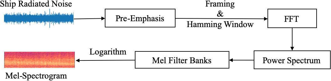
Figure 2 Block diagram of the Mel-spectrogram extraction process. The process mainly includes three stages: (1) the pre-processing stage involves pre-emphasizing, framing and windowing the original signal; (2) the spectrum transformation stage involves N-point Fast Fourier Transform (FFT) on each frame and then computing the power spectrum; (3) the Mel-spectrogram transformation stage aims to apply triangular filters on a Mel-scale to the power spectrum to extract frequency bands and apply logarithm to extract the Mel-spectrogram.

Frequencies are time-varying, so in most cases, applying the Fourier transform to the entire signal would make no sense and lose the frequency contours of the audio data. However, it can be safely assumed that frequencies in a signal are stationary over a very short period. Hence, a good approximation of the frequency contours can be obtained by concatenating adjacent frames’ Fourier transformation results. To avoid variations in a frame, the frame size is usually set small with a millisecond level. In this paper, the frame size of the ship-radiated noise is set to be 25 ms, with feature aggregation conducted over a temporal interval of 75 ms. A Hanning window is used in the work to reduce spectral leakage. Then, a 2048-point FFT with 512 hopping-length in the time domain is applied to each frame in order to generate the frequency spectrum. The power spectrum is computed by Equation 1,

$\begin{array}{ll}P=\frac{{\left|FFT(x_i)\right|}^2}{N}& (1)\end{array}$

where FFT stands for Fast Fourier Transform and x_iis the ith frame of signal x. In the end, the Mel filter bank with 128 bins is applied to the power spectrum to extract the Mel-spectrogram. The rationale behind the choice of 128 is that it is a power of 2, hence it is convenient for the calculations conducted in the neural network. The Hertz(f) and Mel(m) can be converted using Equations 2, 3.

$\begin{array}{ll}m=2595{\log }_{10}(1+\frac{f}{700})& (2)\end{array}$

$\begin{array}{ll}f=700({10}^{m/2595}-1)& (3)\end{array}$

The Mel-scale aims to be more discriminative at lower frequencies and less discriminative at higher frequencies. With a 22050 Hz sampling rate, a 75 ms signal can generate a Mel-spectrogram with the size of 128 × 4. Although the Mel-spectrogram can only reflect the static characteristics of the signal, the duration of each audio signal is short enough to be safely assumed that the target is relatively stable, and therefore, only the static features are mattered. Figure 3 represents an original ship-radiated noise signal and its corresponding Mel-spectrogram.

Figure 3

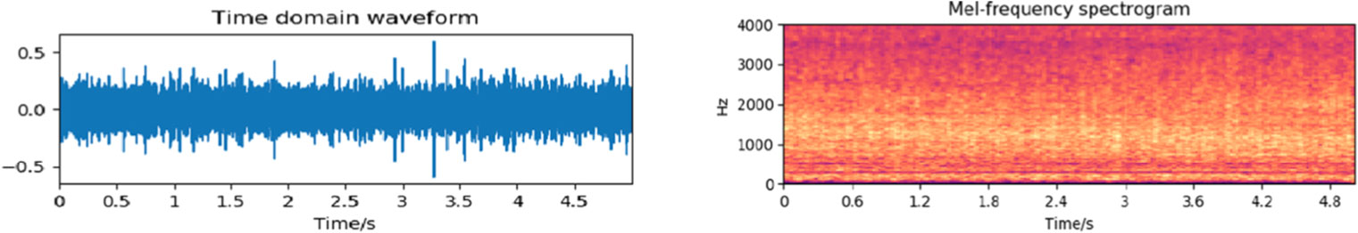
Figure 3 The original signal and its corresponding Mel-spectrogram.

2.3 Model architecture

The overall DWSTr architecture contains two main parts: a DWS block to extract a compact spatial feature representation and a Transformer block to extract timing correlation characteristics. The basic conception of the architecture is inspired by the classical CRNN model with the replacement of a DWS for CNNs, which results in a smaller amount of parameters and increased performance (Ioffe and Szegedy, 2015; Szegedy et al., 2015; Chollet, 2016; Szegedy et al., 2016; Howard et al., 2017), and the replacement of a multi-head attention based Transformer for RNNs, which can perfectly model temporal context and evade the short-term memory problem.

In detail, the proposed model first accepts an input Mel-spectrogram as X ∈ R^T×N×1, where T is 128 and N is 4. The DWS block is mainly composed of a 2D Depthwise convolution layer and a Pointwise convolution layer. Each layer is followed by a normalization process and a rectified linear (ReLU) activation function to overcome the vanishing gradient problem, allowing the model to learn faster and perform better. Figure 4 illustrates the structure. In a typical 2D CNN with unit stride and zero padding, the spatial and cross-channel learning process can be described by Equation 4,

Figure 4

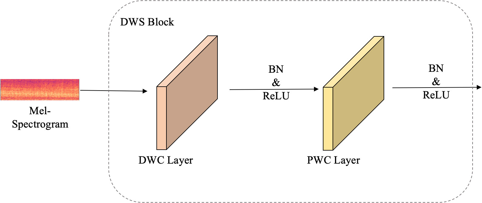
Figure 4 A detailed description of the DWS block. It mainly contains two parts: the DWC (Depthwise Convolution) layer and the PWC (Pointwise Convolution) layer. Each convolution layer is followed by a BN (batch normalization) layer and a ReLU activation layer.

$\begin{array}{ll}{Z}_{x_H^{\text{'}}-K_h,x_W^{\text{'}}-K_w,k_o}=(K_{k_o}*X)(x_h-k_h,x_w-k_w,k_i)={\displaystyle \sum _{k_h}^{K_h}\sum _{k_w}^{K_w}\sum _{k_i}^{K_i}}{X}_{x_h-k_h,x_w-k_w,k_i}{K}_{k_h,k_w,k_o}& (4)\end{array}$

where * denotes the convolution operation. k_i and k_o are the number of input and output channels of the CNN respectively. K_h and K_w represent the height and width of the kernel of each channel. Normally, they are set to be equal to generate a square kernel. Each kernel $K\in R^{K_h\times K_w\times K_i}$ is applied to the input $X\in R^{X_H\times X_W\times K_i}$, then the output $Z\in R^{X_{\text{H}}^{\prime }\times X_{\text{W}}^{\prime }{K}_{\text{o}}}$ is obtained. Its computational complexity is O(K_h · X_H · K_w · X_W · K_i · K_o) and the total number of its learnable parameters is K_h · K_w · K_i · K_o, excluding the bias b ∈ $R^{K_i}$.

Different from traditional CNNs, DWS separates the whole process described above into two parts. Instead of using only one kernel to learn both spatial and cross-channel information in a single convolution, there are two kernels and two convolutions, namely depthwise convolution and pointwise convolution, are employed in series for the input X. At first, K_i kernals $K^s\in R^{K_h\times K_w}$ are applied to each $X_{k_i}$. The learned spatial relationships, $\text{F}\in R^{X_{\text{H}}^{\prime }\times X_{\text{W}}^{\prime }}$, in X can be calculated by Equation 5:

$\begin{array}{ll}{\mathbf{\text{F}}}_{t-K_h,n-K_w,k_i}=({\mathbf{\text{K}}}_{k_o}^s*{\mathbf{\text{X}}}_{{\mathbf{\text{k}}}_{\mathbf{\text{i}}}})(t-K_h,n-K_w)={\displaystyle \sum _{k_h}^{K_h}\sum _{k_w}^{K_w}}{\mathbf{\text{X}}}_{t-k_h,n-k_w,k_i}{\mathbf{\text{K}}}_{k_h,k_w,k_i}^s& (5)\end{array}$

where t = 1,…,T and n = 1,…,N. The result is immediately fed into the second part. K_o kernels are utilized with $K=\{{\text{k}}_1^z,{\text{k}}_2^z,\dots ,k_{{\text{κ}}_o}^z\}$, and are applied to F = {F₁,…,F_Ki}, aiming to extract the cross-channel relationships. The final output is gained based on Equation 6,

$\begin{array}{ll}{\mathbf{\text{Z}}}_{x_H^{\text{'}},x_W^{\text{'}},k_o}={\displaystyle \sum _{k_i}^{K_i}}{\mathbf{\text{F}}}_{x_H^{\text{'}},x_W^{\text{'}},k_i}{\mathbf{\text{K}}}_{k_o,k_i}^z& (6)\end{array}$

It can be concluded that the computational complexity of the DWS is O(K_h · K_h · X_H · K_w · X_W · K_i + $x_{\text{H}}^{\prime }·x_{\text{W}}^{\prime }$ · K_i · K_o). while its total number of parameters is K_h · K_w · K_i+ K_i · K_o.

The reduction in the total number of parameters is:

$\begin{array}{ll}\frac{K_h·K_w·K_i+K_i·K_o}{K_h·K_w·K_i·K_o}=\frac{1}{K_o}+\frac{1}{K_h·K_w}& (7)\end{array}$

Since K_o, K_h and K_w are greater than or equal to 1 by definition, the right side of Equation 7 is less than 1. Hence, the parameters needed are effectively reduced. As for the computational complexity, its change can be expressed as:

$\begin{array}{ll}\begin{array}{l}\frac{K_h·X_H·K_w·X_W·K_i+{x^{\prime }}_H·{x^{\prime }}_W·K_i·K_o}{K_h·X_H·K_w·X_W·K_i·K_o}\\ =\frac{1}{K_o}+\frac{{x^{\prime }}_H·{x^{\prime }}_W}{K_h·X_H·K_w·X_W}\end{array}& (8)\end{array}$

where K_o, K_h and K_w are greater or equal to 1. The $x_{\text{H}}^{\prime }$ and $x_{\text{W}}^{\prime }$ are the input feature dimensions of the pointwise convolution layer. By definition, they are also the output feature dimensions of the depthwise convolution layer. Hence, there will be:

$\begin{array}{ll}{x}_H^{\text{'}}=\frac{X_H-K_h+2Padding}{Stride}+1& (9)\end{array}$

and

$\begin{array}{ll}{x}_W^{\text{'}}=\frac{X_W-K_w+2Padding}{Stride}+1& (10)\end{array}$

In this paper, a unit stride is used along with zero padding. Consequently, Equations 9, 10 are updated to Equations 11, Equations 12, respectively.

$\begin{array}{ll}{x}_H^{\text{'}}=X_H-(K_h-1)& (11)\end{array}$

and

$\begin{array}{ll}{x}_W^{\text{'}}=X_W-(K_w-1)& (12)\end{array}$

Since $K_h$ and $K_w$ are greater than or equal to 1, $x_H^{\text{'}}$ and $x_W^{\text{'}}$ are less than $X_H$ and $X_W$ respectively. Hence, the result of Equation 8 is less than 1, which proves that the DWS can successfully extract spatial features and cross-channel information that is hidden in the input data with less computational costs than traditional CNNs. The process is illustrated in Figure 5.

Figure 5

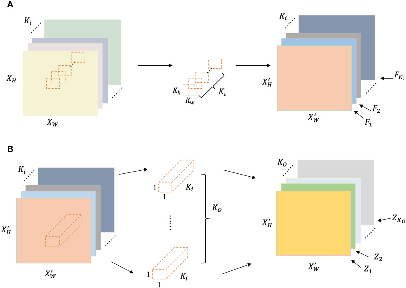
Figure 5 The detailed illustration of the process of the depthwise separable convolution. (A) denotes the role of the depthwise convolution layer: learning spatial information using K_i different kernels from the multi-channel input. (B) denotes the responsibility of the pointwise convolution layer: learning cross-channel information using K_odifferent kernels.

By reconstructing the input sample, the DWS network can effectively extract spatial characteristics contained in the spectrogram without destroying the structure information. However, the temporal features hidden in the ship-radiated noise remain un-highlighted. In order to achieve better recognition results, a Transformer is connected to the DWS block. The standard Transformer receives each input as a one-dimensional sequence of embedded tokens. In order to handle the two-dimensional feature maps generated by the DWS, a patch embedding projection is employed to reshape the input feature maps $Z\in R^{x_H^{\text{'}}\times x_W^{\text{'}}\times K_o}$ into sequences of flattened 2D patches $Z_p\in R^{N\times (P_H·P_W·K_o)}$, where P_H and P_W are the height and width of each patch and they are usually set to be equivalence. $N=(x_H^{\text{'}}{x}_W^{\text{'}})/(P_H·P_W)$ is the total number of patches, which also serves as the effective input sequence length for the Transformer. Hence, every input sequence can be obtained by simply flattening the spatial dimensions of the feature map and projecting to the Transformer dimension. Subsequently, a learnable class embedding is prepended to the sequence and a position embedding tensor is tailed to the sequence aiming to preserve the feature map’s positional information. Together, the position annotated sequence serves as input to the Transformer’s encoder, where all the patches can be parallelly received and encoded. Although the input feature maps are batched together, their dimensions are the same, ensuring that parallel computing can go without a hitch. The process can be expressed by Equation 13,

$\begin{array}{ll}{\mathbf{\text{Z}}}_0=[{\mathbf{\text{Z}}}_{class};{\mathbf{\text{Z}}}_p^1\mathbf{\text{E}};{\mathbf{\text{Z}}}_p^2\mathbf{\text{E}};\cdots ;{\mathbf{\text{Z}}}_p^N\mathbf{\text{E}}]+{\mathbf{\text{E}}}_{pos}& (13)\end{array}$

where E is the trainable patch embedding, which flattens the patches and projects them to the Transformer dimension. E_pos is the learnable position embedding. It learns each patch’s positional information in the sequence so that even if the input feature mapping is dimensionality deducted, reshaped, and segmented, its higher dimensional lexeme can be mostly retained. The class token Z_class serves as a label of the linearly flattened sequence. It is always placed in the very first place to ensure that the Transformer can find it every time without going through the entire sequence.

In the following step, the model learns more abstract features from the embedded patches using a stack of transformer encoders. The encoder consists of alternating layers of self-attention and MLP. Layer normalization (LN) is applied before every layer and layers are connected by residual connections. The multi-head attention (MHA) is employed rather than the single head attention in the encoder. Because MHA allows the model to perform attention multiple times in parallel which results in better performance and richer information extracted from different representation subspaces. The procedure is encapsulated by Equations 14, 15, with Equation 14 illustrating the comprehensive process and Equation 15 specifying the operation within a single head. For each patch in the input sequence, an attention weight A is calculated. The attention score is based on the pairwise similarity between two patches of the sequence and their respective query q and key k representations. Its calculation process can be expressed as Equation 16:

$\begin{array}{ll}\begin{array}{ll}MHA({\mathbf{\text{Z}}}_{l-\mathbf{1}})\hfill & =[hea{d}_1;hea{d}_2;\dots ;hea{d}_m]{\mathbf{\text{W}}}^o\hfill \\ ={\displaystyle \sum _i^m}hea{d}_i{W}_i^o\hfill \end{array}& (14)\end{array}$

$\begin{array}{ll}hea{d}_i=softmax(\mathbf{\text{q}}{\mathbf{\text{k}}}^{\mathit{\text{T}}}/\sqrt{d})v& (15)\end{array}$

$\begin{array}{ll}[q,k,v]={\text{Z}}_{l-1}{U}_{qkv}& (16)\end{array}$

where, both W° and U_qkv are learnable matrices. Z_l−1 denotes the output generated from the former layer and d is usually set to be equal to the hidden dimension of the patch’s key representation.

By applying the MHA mechanism, the salient time correlation features hidden between frames can be efficiently obtained. Although recurrent layers used in RNNs are also good at extracting the temporal features from the sequential data, the MHA can do it much faster. As noted in Table 1, if an input sequence length is n, then a Transformer with a self-attention mechanism layer will have access to each element with O(1) sequential operations whereas an RNN with a recurrent layer will need O(n) sequential operations to access an element. With O(n) sequential operations and under the influence of the chain rule in the backward propagation calculation process, long sequences will cause problems with exploding and vanishing gradients. However, the Transformer does not suffer from the gradient problem, since the distance to each element in the sequence is always O(1) sequential operations away. In this paper, n is the total number of patches N = 13, which is considerably smaller than the representation dimension d = 14 × 14. Hence, by employing the attention method rather than the recurrent method, the computational complexity can be greatly reduced.

Table 1

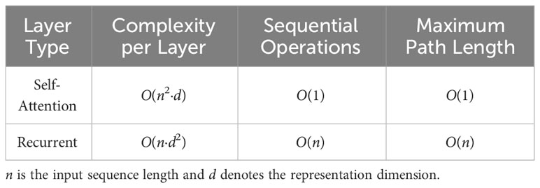
Table 1 Complexity comparison between the self-attention layer and the recurrent layer.

The attention score is then sent to a simple, position-wise fully connected feed-forward neural network, MLP. It normalizes the outputs and aids in learning during backpropagation via residual connections. The other sub-layers help to stabilize the network while deepening the model so that the problem of vanishing gradients can be avoided. The outputs of the Transformer encoder are sent into a classification head. It is implemented by an MLP with one hidden layer and it receives the value of the learnable class embedding, namely the class token, to generate a classification output based on its state. The entire set of processes is delineated from Equations 17–19

$\begin{array}{ll}{Z}_l^{\text{'}}=MHA(Z_{l-1})+Z_{l-1}& (17)\end{array}$

$\begin{array}{ll}{Z}_l=MLP(LN(Z_l^{\text{'}}))+Z_l^{\text{'}}& (18)\end{array}$

$\begin{array}{ll}Y=LN(Z_{class})& (19)\end{array}$

Besides the linear normalization layers, dropout layers are also employed to optimize the network structure. Furthermore, in order to verify the best result and select the most suitable network structure, different combinations of layer construction and parameters are tested; the detailed test results will be described in the next section. In the proposed network structure, the DWS block is used for the extraction of spatial characteristics and the Transformer block is responsible for abstracting temporal features from Mel-spectrograms.

3 Experiment

3.1 Dataset

The underwater vessel noise dataset used in this paper is ShipsEar (Santos-Domínguez et al., 2016). Each acoustic signal sample is recorded in real oceanic conditions and therefore contains certain natural or anthropogenic environment noise. There are 90 acoustic samples representing 11 vessel types in the dataset. Each category contains one or more samples and the audio length of each sample varies from 15 seconds to 10 minutes. In the experiments, the dataset was split into a training set, a testing set, and a validation set. 70% of the ShipsEar’s data went to the training set, which was used for model training and fitting. 20% was used to tune the model’s hyperparameters and make an initial assessment of the model’s capabilities. The last 10% formed the validation set and it was kept unknown for the model while training and testing in order to evaluate the generalization ability and robustness of the final model. Since during the data preprocessing period a slicing method is employed to cut all signals according to a fixed duration of 75 milliseconds, the dataset is augmented and it becomes large enough for every category’s data can be split into three sets. All the samples are randomly selected and separated into different sets according to the ratio.

3.2 Training and testing

In this paper, the training and testing of the proposed model were conducted utilizing Nvidia’s RTX3090 GPU, which is equipped with 24 GB of G6X memory. The parameters used during the training and testing stages are listed in Table 2 while Figure 6 provides a detailed view of the model’s performance in each epoch of these stages.

Table 2

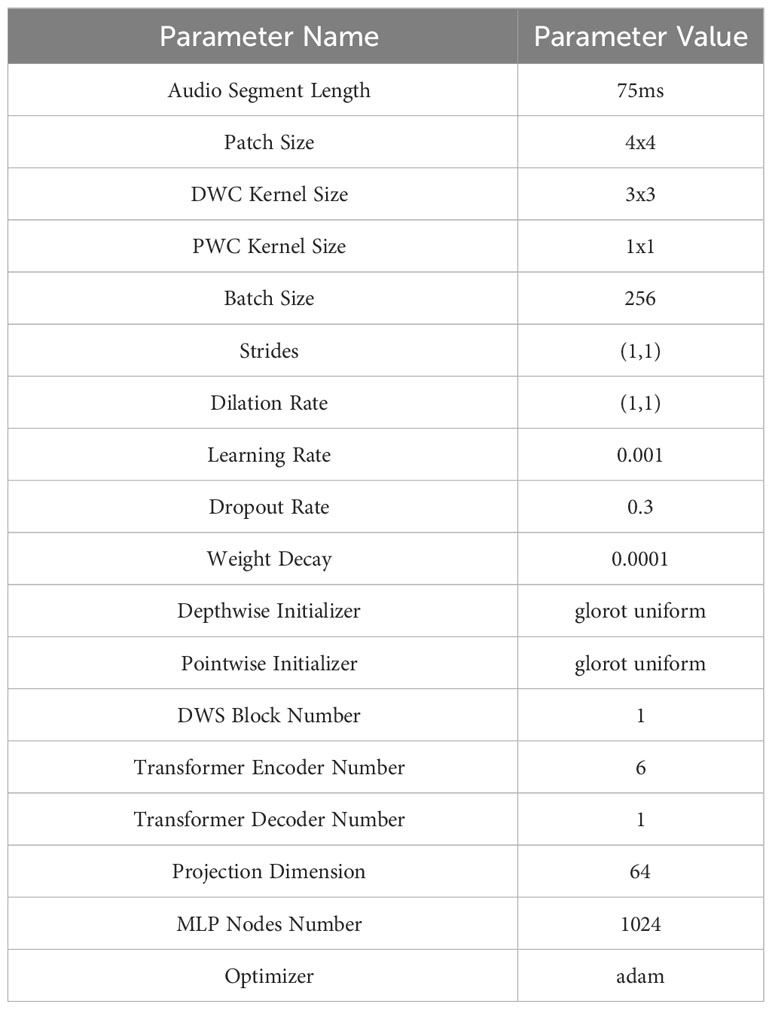
Table 2 The following parameters are utilized in the proposed model during both the training and testing stages.

Figure 6

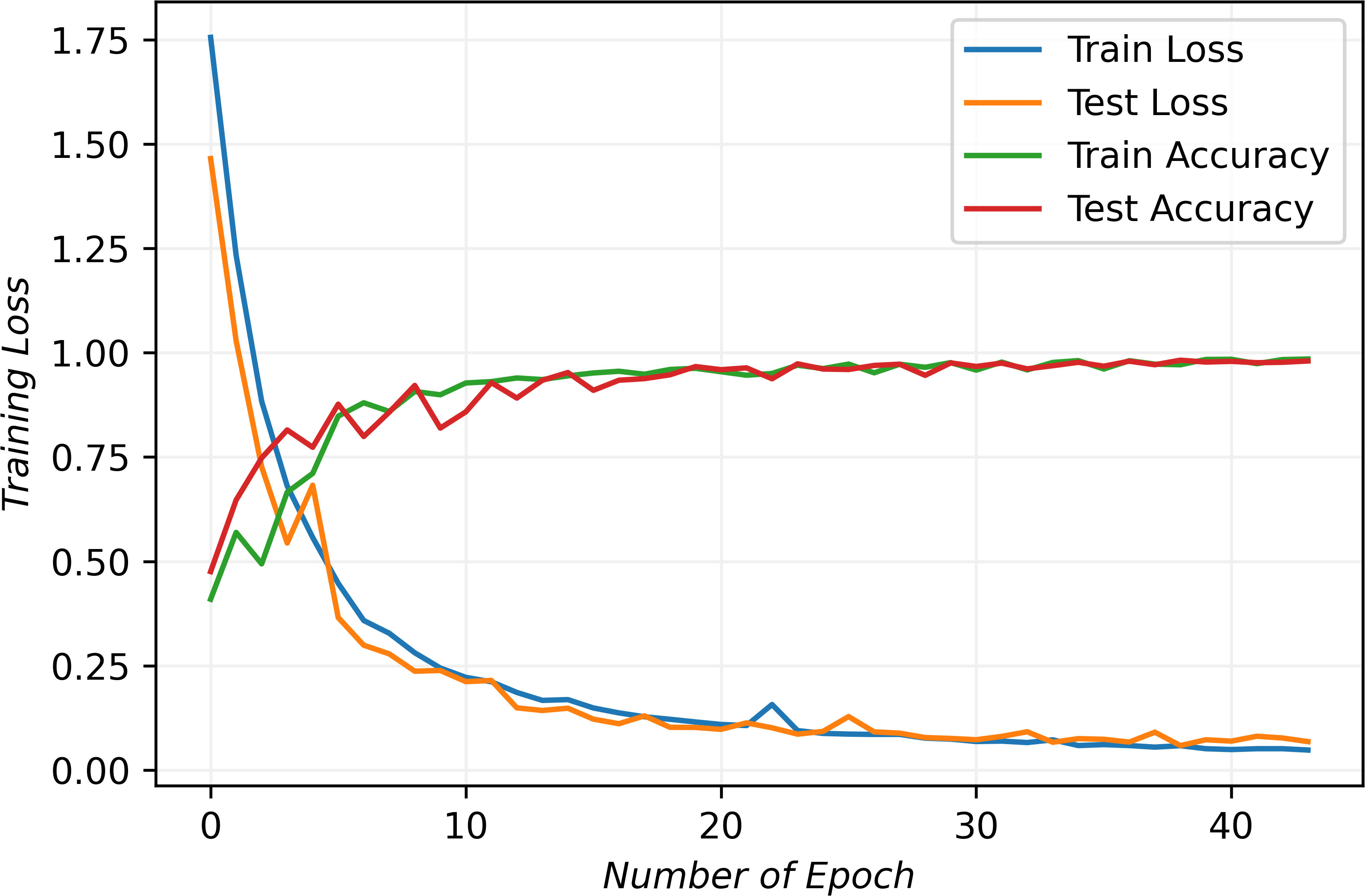
Figure 6 The detailed training process and results. The tendency of lines indicates an optimal fit.

The initial assessment of a deep learning model typically involves analyzing training and testing losses, which measure the errors for each example in their respective datasets. As depicted in the figure, both training and testing losses exhibit a decreasing trend, while training and testing accuracies steadily increase. They start to stabilize after ten epochs and stop after fourteen epochs. The behavior indicates the model’s effective convergence to an optimal fit.

Overfitting and underfitting are common challenges in deep learning which often arise when the model struggles to generalize well on new data or experiences significant errors in the training data. These issues often result in diverging loss lines due to gradient disappearance or explosion. However, as evident from the figure, the convergence lines of the proposed model demonstrate its capability to mitigate these problems and effectively learn the underlying data features. Consequently, the results demonstrate our model’s high performance and its potential as a robust data analysis and prediction tool.

3.3 Evaluation

In order to find the optimal number of DWS blocks needed for the model to extract and learn the spatial features from the raw data, different numbers of DWS blocks were tested. Figure 7 exhibits the results. In both the training and testing process, a single DWS block achieved the best results.

Figure 7

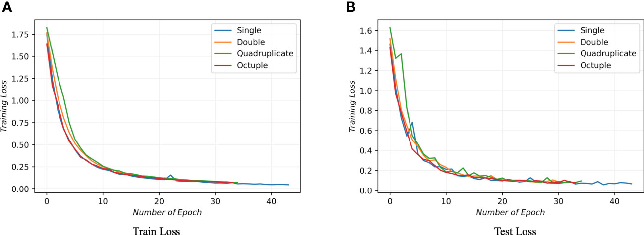
Figure 7 This figure illustrates the variance in model performance with different numbers of DWS blocks during training, evaluating configurations with 1, 2, 4, and 8 DWS blocks. Subfigure (A) illustrates the performance throughout the training phase, whereas Subfigure (B) highlights the performance during the testing phase. The findings reveal that the model achieves optimal learning efficiency when equipped with a singular DWS block.

While with the number of DWS blocks determined, the number of Transformer blocks also needs to be tested not only for the purpose of achieving better identification accuracy but also aiming to optimize the utility of computational resources. As shown in Figure 8, the ideal depth, 6, was founded after several thorough experiments.

Figure 8

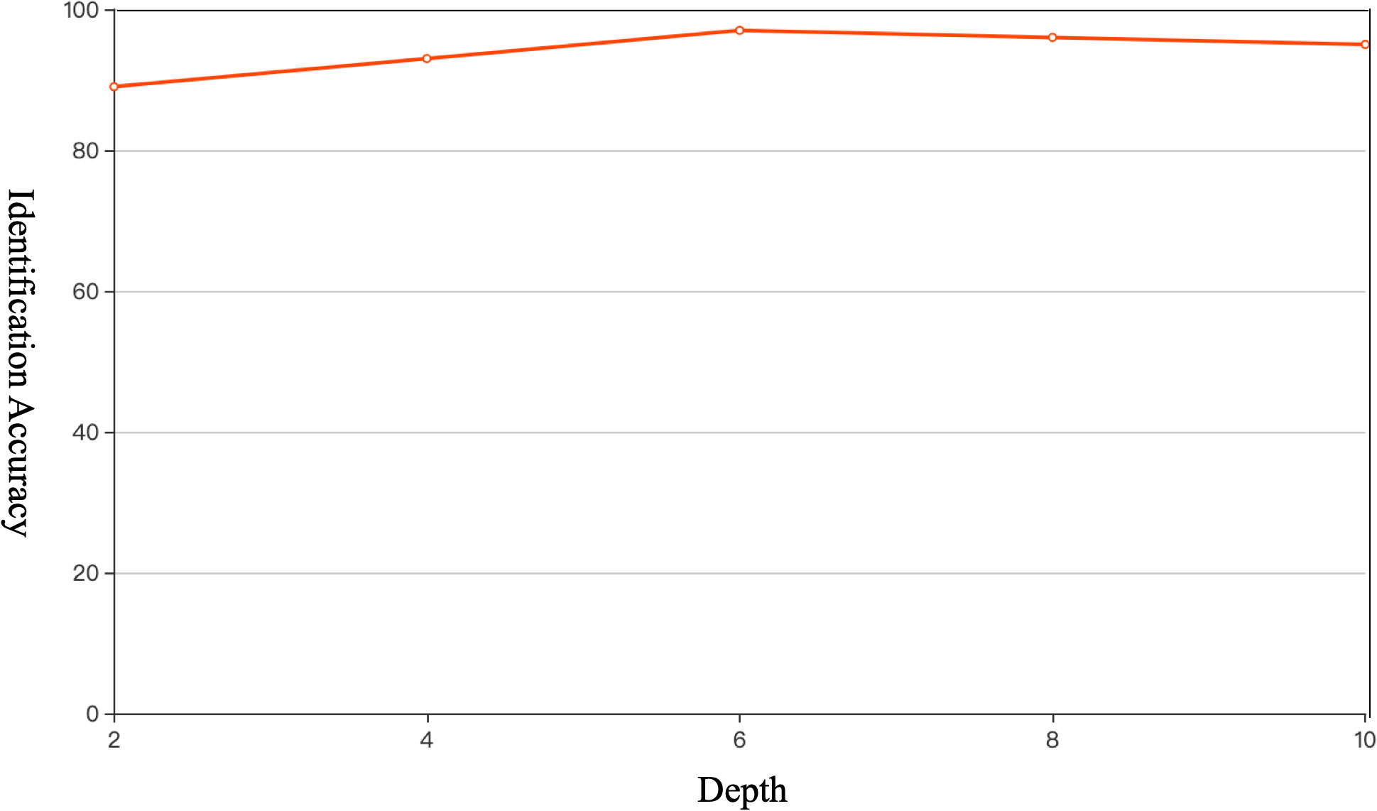
Figure 8 Model performance comparison in different numbers of Transformer blocks. The optimal quantity of Transformer blocks is 6.

Figure 9 describes different classification accuracies with different patch sizes, batch sizes and audio segment lengths. The patch size represents the size of the patches to be extracted from the input data by the transformer block. Since the Transformer’s sequence length is inversely proportional to the square of the patch size, models with smaller patch sizes are computationally more expansive. However, a larger patch size does not necessarily indicate a better result. A larger patch size leads to a smaller number of patches for the same input, meaning fewer learning chances and worse results, as can be seen from the comparison in Figure 9.

Figure 9

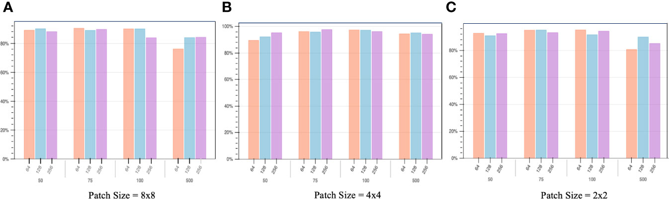
Figure 9 The study meticulously evaluates identification accuracy by examining a range of patch sizes, batch sizes, and audio segment durations. The classification accuracy is plotted on the y-axis, while the x-axis is organized into two levels: the first level delineates the patch sizes, and the second level outlines the lengths of the audio segments. Subfigure (A) illustrates the variance in performance for an 8x8 patch size across diverse audio segment durations and batch sizes. Subfigure (B) explores the performance implications of employing a 4x4 patch size, again across varying audio segment durations and batch sizes. Subfigure (C) delves into the performance metrics associated with a 2x2 patch size under different audio segment durations and batch sizes. The analysis concludes that the configuration yielding the highest accuracy involves a 4x4 patch size, combined with a batch size of 256 and an audio segment duration of 75ms.

Another element that should be considered is the model’s batch size. It defines the number of samples to work through before updating the internal model parameters. Batch size is commonly kept in the power of 2 because the number of GPUs’ physical processors is often a power of 2. Using a number of virtual processors different from the number of physical processors will lead to poor performance. The 50, 75, 100, and 500 indicate different lengths of audio clips in milliseconds. As shown in the figure, while patch size = 4x4, audio segment length = 75, and batch size = 256, the classification accuracy reaches the ideal result, approximately 96.5%. The promising result proved that even working with milliseconds-long audio clips recorded in an extremely challenging environment, the proposed model can accurately identify the vast majority of them. The detailed graphical representation of each class’s recognition result is shown in Figure 10.

Figure 10

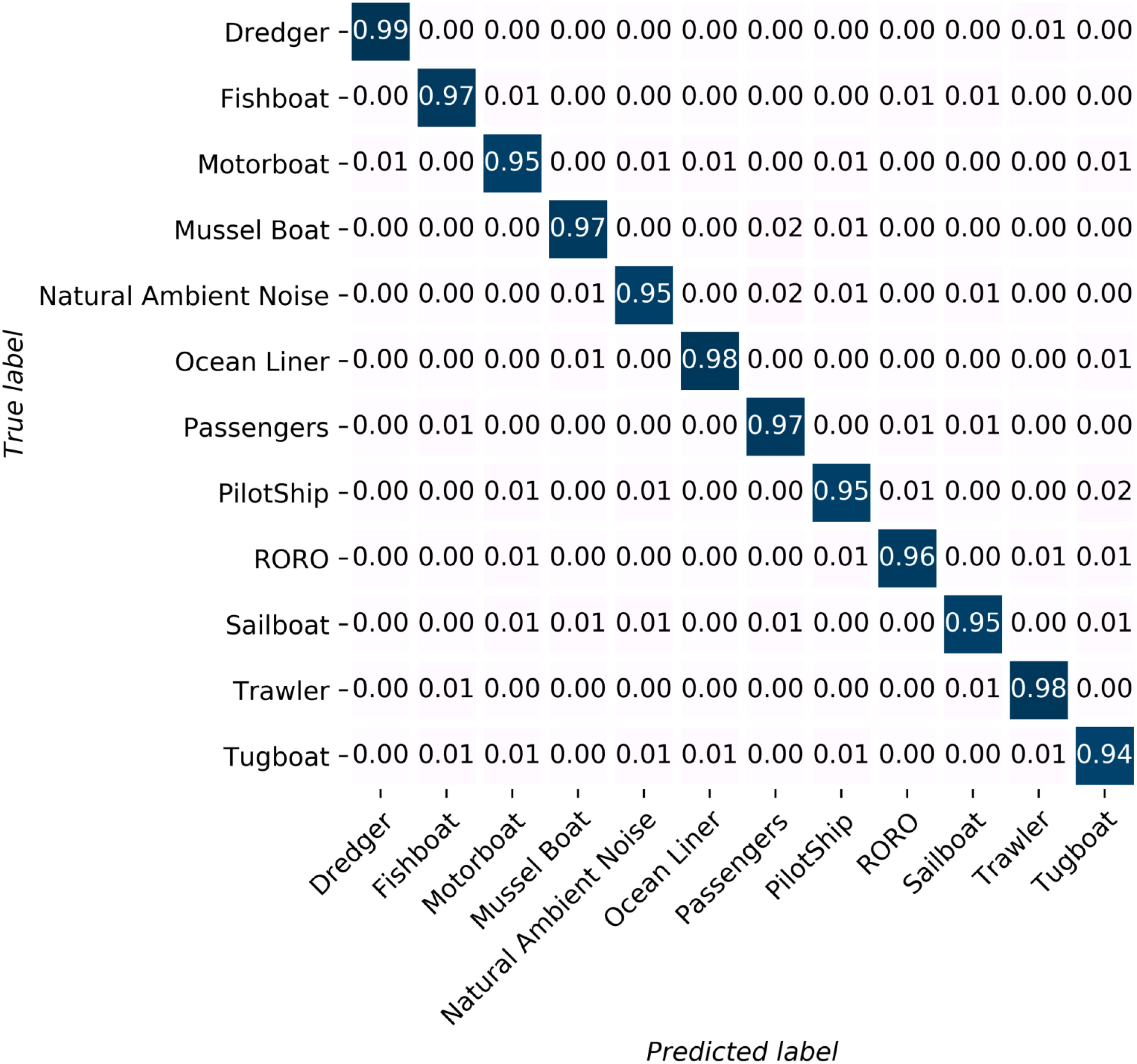
Figure 10 Each class’s identification result. All of the categories own an identification accuracy higher than 94%. Seven out of twelve categories’ identification accuracy is higher than 95%.

Figure 11 shows the classification performance by selecting different optimizers and different dropout rates. Figure 11 offers insights into our model’s classification performance, considering various optimizers and dropout rates. Optimizers play a pivotal role in parameter updates based on loss gradients. We assessed five common optimizers: adaptive moment estimation (Adam), root mean square propagation (RMSprop), stochastic gradient descent (SGD), adaptive gradient (Adagrad), and adaptive delta (Adadelta). Our results, depicted in Figure 11, demonstrate that Adam excels when applied to non-convex underwater signal datasets. Underwater acoustic signals are often sparse and noisy, making accurate gradient estimation challenging. Adam and RMSprop both adapt learning rates using historical gradient data, making them effective in handling sparse and noisy gradients. Their adaptability ensures stable and efficient optimization under such conditions. Adam, which combines momentum and adaptive learning rates, maintains separate learning rates for each parameter, employing adaptive estimates of first and second-order gradient moments. RMSprop also adapts learning rates but only considers first-order gradient moments, making it slightly less effective than Adam in handling underwater acoustic data.

Figure 11

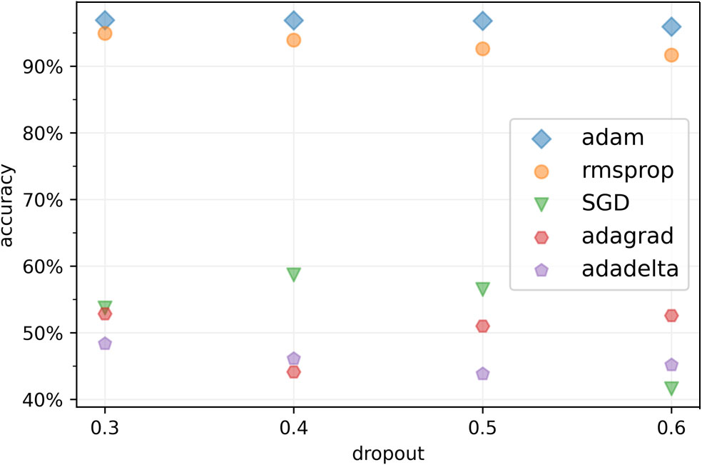
Figure 11 Comparison of different identification accuracies in different optimizers and dropouts. The Adam optimizer reaches the local minimum most effective in the ship target recognition task while the dropout rate should set to 0.3 to achieve the optimal result.

Conversely, SGD’s fixed learning rate often leads to slow convergence and can be sensitive to the choice of learning rate. The rigidity of this rate prevents automatic adjustments, possibly causing oscillations or divergence with high learning rates and slow convergence or suboptimal solutions with low learning rates. Adadelta struggles with sparse gradients, limiting its parameter updates and demanding higher memory due to squared gradient accumulation. Adagrad’s declining learning rates over time can hinder adaptation in underwater acoustic target recognition, with the accumulation of historical gradients potentially diminishing the relevance of recent gradient data.

Dropout, a regularization technique, randomly deactivates nodes within a layer during training to combat overfitting. Our experiments have revealed an optimal dropout rate of 0.3, excluding approximately one-third of inputs during each update iteration.

A dropout rate below 0.3 can cause overreliance on specific nodes, undermining the model’s capacity to learn diverse representations and hampering its generalization. Conversely, a dropout rate above 0.3 can impair learning complex patterns and relationships, resulting in decreased performance.

In Figure 12, the recognition results of several comparison models are shown. The different colors indicate CRNN (Convolutional and Recurrent Neural Network) (Hu et al., 2023), DBNs (Deep Belief Networks) (Yang et al., 2018), Swin-Transformer (Chen et al., 2022), SAEs (Sparse Autoencoders) (Ke et al., 2018), and MobileNet (Mobile Network) (Liang et al., 2020) respectively. The primary parameters for the comparative models are comprehensively listed in Table 3. These settings conform to the methodologies specified in the respective research papers whenever available. In cases where such specific settings are not provided in the referenced literature, the models adhere to the parameters established by the proposed method.

Figure 12

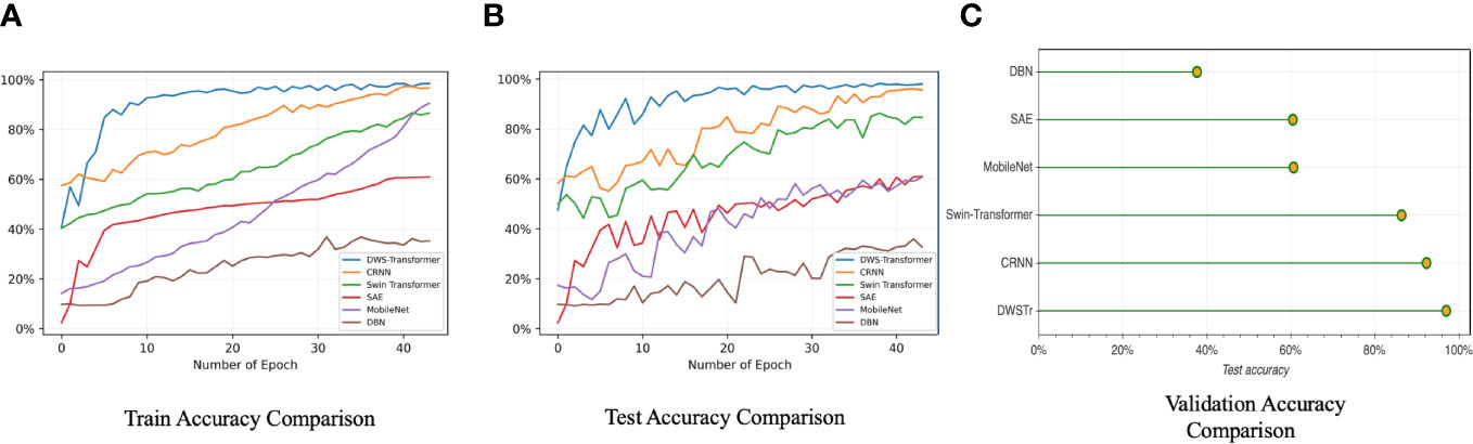
Figure 12 The comparison highlights the identification accuracy between the proposed model and other prevalent neural networks. In subfigures (A, B), the y-axis quantifies classification accuracy, whereas in subfigure (C), it directly measures accuracy. Various colored lines within (A, B) correspond to the different models evaluated. The proposed model outperforms others in training, testing, and validation phases, reaching optimal results faster. Notably, at the same epoch count, the proposed model has converged to its peak performance, whereas competing models continue to evolve.

Table 3

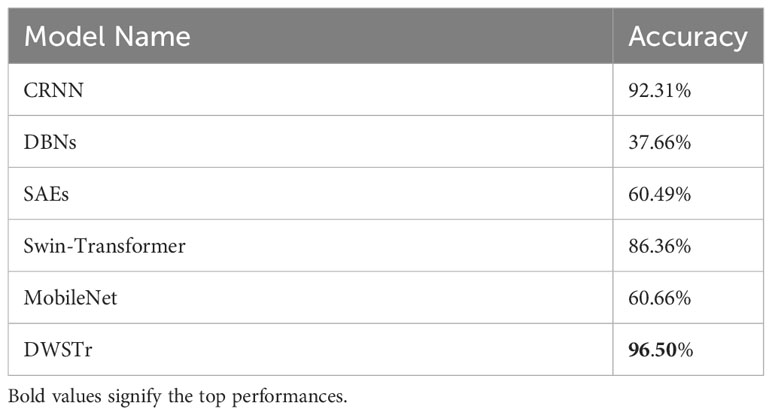
Table 3 Numerical accuracy comparison.

The numerical classification accuracy for each comparison model is systematically tabulated in Table 4, facilitating a direct comparison of their respective performances. It is observed that neural networks with a singular focus on either local or global information processing tend to lag behind those capable of integrating both aspects. This emphasizes the significance of a dual approach in handling local and global information for achieving superior classification results in neural network models.

Table 4

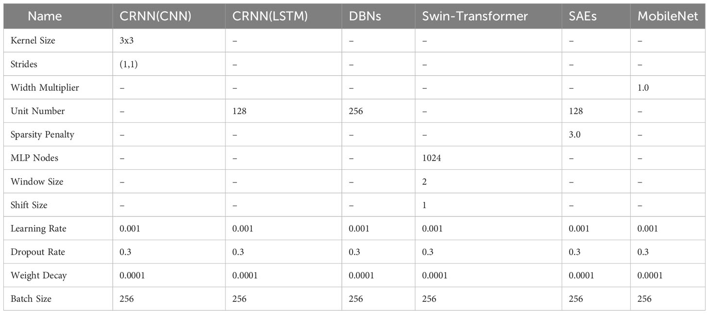
Table 4 The following parameters are utilized in the comparison models. CRNN(CNN) represents the convolutional component, while CRNN(LSTM) denotes the recurrent segment of the model.

Ship-radiated noise classification is a challenging task due to the complex and noisy nature of underwater environments. The acoustic signals radiated by ships are often masked by natural sounds, attenuated, and distorted, making it difficult for models to extract relevant acoustic features. The CRNN is a powerful model for various sequence-related tasks. However, when applied to shipradiated noise recognition tasks, it can have certain deficiencies that may diminish its performance. While RNNs can capture sequential information, they can struggle to capture very long-term dependencies. Ship-radiated noise can have complex patterns and dependencies that span over a considerable time frame. CRNNs, which combine CNNs for feature extraction and RNNs for sequence modeling, might not effectively capture these long-range dependencies.

Ship-radiated noise is a time-dependent signal with intricate temporal patterns. DBNs are primarily designed for modeling static data distributions and may not effectively capture the temporal dependencies present in audio signals. This deficiency can limit their ability to discern relevant noise patterns over time. Furthermore, DBNs are feedforward networks, which means they lack inherent sequential learning capabilities. Ship-radiated noise recognition often involves identifying patterns and trends in the noise signal over time. DBNs may struggle to capture these sequential dependencies without additional modifications.

While Swin-Transformer is a promising architecture that has shown effectiveness in various computer vision tasks, it may face certain deficiencies when applied to ship-radiated noise recognition tasks, which could potentially diminish its performance. Ship-radiated noise is a time-dependent signal with intricate temporal patterns. Swin-Transformer primarily excels in processing spatial information in spectrograms. Its attention mechanism, while powerful for spatial relationships, may not be optimized for capturing the temporal dynamics present in audio signals. This limitation can hinder its ability to effectively recognize ship noises over time.

The sparsity constraints in SAEs may make them less suitable for tasks where the acoustic features don’t naturally lend themselves to sparse representations. Ship-radiated noise recognition often involves recognizing complex sound patterns, and forcing sparsity in the feature space might not align with the underlying data distribution. This can lead to suboptimal performance when compared to other techniques that don’t enforce sparsity.

MobileNet is a neural network architecture known for its efficiency and effectiveness. However, when applied to the ship-radiated noise recognition task, it may face several deficiencies that can impact its performance. MobileNet architectures typically involve depthwise separable convolutions, which reduce computational complexity and model size. While this is advantageous for mobile and embedded devices, it may not provide the necessary model capacity for ship-radiated noise recognition. Recognizing different ship noise categories in various environmental conditions requires a model with sufficient capacity to learn intricate patterns. MobileNet’s lightweight design, while efficient, might struggle with capturing the complex and diverse acoustic features in ship noise, leading to reduced recognition accuracy.

The running speed of each model, as detailed in Table 5, is a critical factor to consider, reflecting the model’s computational complexity. While our proposed model may not exhibit optimal performance during the training and testing phases, it excels in the validation phase, indicating superior real-time analysis capability. This aspect is particularly significant as it determines the model’s practical applicability in real-world scenarios, where efficient and timely processing of data is essential. Therefore, balancing computational efficiency with performance is key in developing effective and deployable models.

Table 5

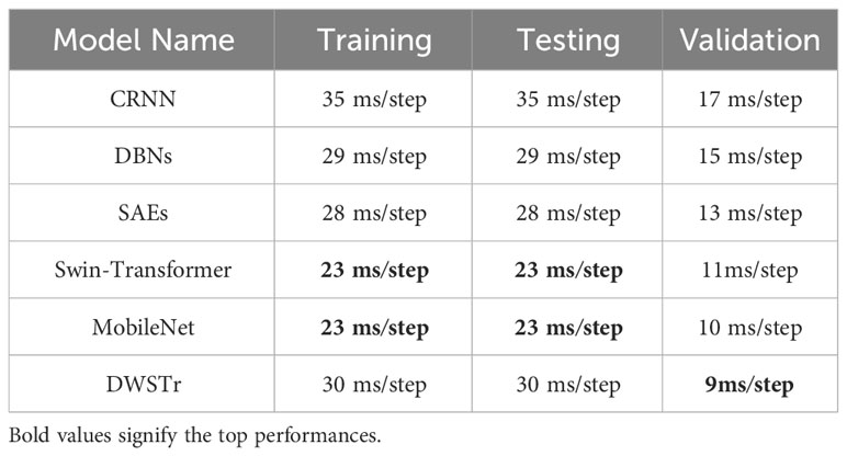
Table 5 Running speed comparison.

DWSTr presents a compelling solution for ship-radiated noise recognition due to its unique combination of DWS and Transformer components. The DWS component specializes in extracting local acoustic features, allowing it to distinguish relevant information from interference. Simultaneously, the Transformer framework captures global and long-range dependencies in the data, helping mitigate the effects of interference, distortion, and variability in noise signatures. This dual capability enables DWSTr to excel in handling ship noise recognition tasks, where both local and global features play a crucial role in accurate classification. Hence, as shown above, using the same dataset to fulfill the same task, DWSTr can achieve the best result.

3.4 Ablation experiments

To ascertain the efficacy of the proposed model, four distinct models were conceptualized and employed in ablation studies. These models are systematically designed to evaluate specific components and functionalities within the overall architecture, thereby enabling a comprehensive analysis of the proposed model’s performance. The following outlines the specifics of the four models.

• DWSTr-CNN: In this variant of the model, traditional CNNs are utilized instead of the DWS block. This adaptation serves as a crucial experiment to evaluate the impact of the DWS block on feature extraction and the overall performance of the model.

• DWSTr-DWS: In this altered model, the Transformer framework is omitted to solely concentrate on the functionality of the DWS component. This change provides a focused analysis on how the DWS block performs independently in the model’s architecture.

• DWSTr-Tr: This model variation, by excluding the DWS block, focuses on assessing the Transformer’s proficiency in managing global and long-range dependencies within the data. This approach allows for a targeted evaluation of the Transformer’s capabilities in isolation.

• Baseline DWSTr: The full DWSTr model is utilized as the benchmark for comparison in the ablation experiments, providing a comprehensive standard against which the performance of each variant model is assessed.

For a thorough and equitable assessment, each model variant undergoes evaluation using an identical dataset and a uniform set of performance metrics. The results of these evaluations, which provide critical insights into the comparative effectiveness of each model, are systematically documented in Table 6. For the DWSTr-CNN model, the comparative analysis reveals a nominal decrease in accuracy and a prolongation in computation time vis-à-vis the baseline DWSTr framework. This phenomenon is attributed to the intrinsic characteristics of conventional CNNs. While they exhibit adeptness in feature extraction, their efficiency, particularly in terms of parameter optimization and local feature processing, falls short when compared to the DWS mechanism. This discrepancy results in a slight compromise in the model’s overall efficiency and its capacity for feature extraction.

Table 6

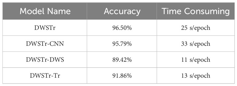
Table 6 Experimental results of the ablation models.

For the DWSTr-DWS model, the observed results reveal a reduced efficiency, likely stemming from its limited ability to capture global dependencies. This limitation notably impacts the model’s overall accuracy. Such a reduction in performance suggests that the global contextual understanding, crucial for comprehensive signal analysis, is not optimally harnessed in this model variant. This finding underscores the importance of effectively integrating mechanisms within the model that proficiently handle global dependencies, thus reinforcing the necessity for a balanced approach in local and global feature analysis in complex signal recognition tasks.

The DWSTr-Tr model is particularly proficient in global feature analysis, effectively discerning broad patterns and dependencies. This capability is especially valuable for classifying ship noise, a domain where recognizing overarching acoustic patterns is critical. However, the model’s capability in processing detailed local features is less pronounced, leading to a slight reduction in accuracy. This underscores the necessity of balancing global and local feature analysis in complex acoustic signal processing, highlighting the importance of a model architecture that effectively integrates both macro-level contextual understanding and micro-level detail recognition.

3.5 Verification experiments

Due to the sensitive nature of ship-radiated noise data, only two public datasets, ShipsEar and DeepShip, are available. For a comprehensive validation of our model, we integrated DeepShip (Irfan et al., 2021) into our analysis. DeepShip encompasses 47 hours and 4 minutes of varied underwater recordings from 265 vessels in four classes: Cargo, Passenger Ship, Tanker, and Tugboat. Recorded between May 2016 and October 2018 at the Strait of Georgia delta node, it presents a diverse environment compared to ShipsEar’s data from Spain, collected between 2012 and 2014.

Before being processed by the models, each audio recording is segmented into 75-millisecond clips, following the same preprocessing approach that was applied to the ShipsEar dataset. Additionally, the hyperparameters used in the verification experiments remain consistent. The classification results are shown in Figure 13.

Figure 13

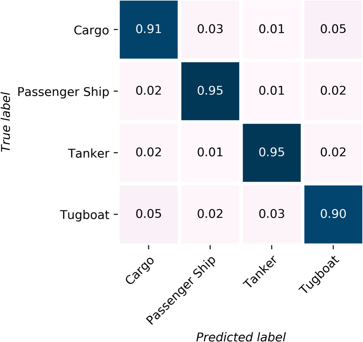
Figure 13 Categorical classification accuracy for the DeepShip dataset.

While no individual category in the DeepShip dataset surpasses a classification accuracy of 95%, the lowest recorded accuracy is a commendable 90%. Notably, the Tugboat and Passenger Ship categories are common to both the DeepShip and ShipsEar datasets, showing consistent classification results. In particular, the Passenger Ship class achieves relatively high accuracy in both datasets when analyzed with the DWSTr model. However, the classification accuracy for Tugboats is the lowest in both datasets. This lower performance could be attributed to data scarcity, as Tugboats constitute approximately only 2.2% of the ShipsEar and 11% of the DeepShip dataset, compared to Passenger Ships, which represent about 33% in ShipsEar and 31% in DeepShip. The overall accuracy of the model on the DeepShip dataset is approximately 92.75%, underscoring its robustness and adaptability across different datasets.

4 Conclusion

In this study, we introduce a hybrid neural network model, named as DWSTr, which integrates a convolutional neural network with a Transformer framework to address the challenge of shipradiated noise identification. The model’s efficacy was rigorously evaluated through experiments, demonstrating its capacity to robustly extract features from input data and achieve accurate classification of underwater acoustic targets, even with signal data lasting mere milliseconds. Comparative analysis reveals that DWSTr surpasses conventional models like CRNN, DBNs, Swin-Transformer, SAEs, and MobileNet, commonly employed in underwater acoustic signal classification. Specifically, DWSTr attains a remarkable classification accuracy of 96.5% on the ShipsEar dataset, coupled with an impressive validation speed of 9 ms/step, suggesting its potential for real-time application. Across the ShipsEar dataset, the model consistently achieves identification accuracies above 94%, with more than half of the categories exceeding 95%, indicative of its overall superior performance.

To further investigate the architecture’s efficacy, ablation studies were conducted. Ship-radiated noise, encapsulating both temporal and spectral dimensions, necessitates a model capable of comprehensive time-frequency analysis. The absence of either the DWS or Transformer blocks resulted in a decrease in accuracy to 91.86% and 89.42%, respectively, underscoring the significance of both components in the model. Moreover, the inclusion of the DWS block notably enhanced the model’s computational speed. Substituting it with a traditional CNN block, while only slightly affecting accuracy, led to a significant increase in computational time, from 25 s/epoch to 33 s/epoch.

Beyond the ShipsEar dataset, the model’s robustness was validated using the DeepShip dataset, which comprises recordings from a distinct location and time period. DWSTr achieved commendable classification accuracies for Cargo, Passenger Ship, Tug, and Tanker classes, with respective scores of approximately 91%, 95%, 95%, and 90%, further affirming its robustness and versatility. Given the model’s exceptional performance, we posit that the DWSTr is well-suited for a broad spectrum of underwater acoustic signal classification tasks.

Data availability statement

The original contributions presented in the study are included in the article/supplementary materials, further inquiries can be directed to the corresponding author/s.

Author contributions

YW: Writing – original draft. HZ: Writing – review & editing. WH: Writing – review & editing. MZ: Writing – review & editing. YG: Writing – review & editing. YA: Writing – review & editing. HJ: Writing – review & editing.

Funding

The author(s) declare financial support was received for the research, authorship, and/or publication of this article. This work was financially supported by National Natural Science Foundation of China (NSFC:62271459), National Defense Science and Technology Innovation Special Zone Project: Marine Science and Technology Collaborative Innovation Center (22-05-CXZX-04-01-02), the Qingdao Postdoctoral Science Foundation (QDBSH20220202061), the Fundamental Research Funds for the Central Universities, Ocean University of China (202313036), the Shandong Provincial Natural Science Foundation (ZR2021QD089) and the Fundamental Research Funds for the Central Universities (202113040).

Conflict of interest

The authors declare that the research was conducted in the absence of any commercial or financial relationships that could be construed as a potential conflict of interest.

Publisher’s note

All claims expressed in this article are solely those of the authors and do not necessarily represent those of their affiliated organizations, or those of the publisher, the editors and the reviewers. Any product that may be evaluated in this article, or claim that may be made by its manufacturer, is not guaranteed or endorsed by the publisher.

References

Alzaq H., Üstündağ B. B. (2018). “A comparative performance of discrete wavelet transform implementations using multiplierless,” in Wavelet theory and its applications (Prolaz Marije Krucifikse Kozulić 2. 51000 Rijeka - Croatia: IntechOpen), 111.

Google Scholar

Brown T., Mann B., Ryder N., Subbiah M., Kaplan J. D., Dhariwal P., et al. (2020). Language models are few-shot learners. 33, 1877–1901.

Google Scholar

Chen C., Li Z., Lu L. (2017). Underwater acoustic signal classification using deep convolutional neural networks. IEEE J. Oceanic Eng. 42, 964–971. doi: 10.1109/JOE.2016.2609380

CrossRef Full Text | Google Scholar

Chen J., Han B., Ma X., Zhang J. (2021). Underwater target recognition based on multidecision lofar spectrum enhancement: A deep-learning approach. Future Internet 13. doi: 10.3390/fi13100265

CrossRef Full Text | Google Scholar

Chen K., Du X., Zhu B., Ma Z., Berg-Kirkpatrick T., Dubnov S. (2022). HTS-AT: A hierarchical token-semantic audio transformer for sound classification and detection. Available at: arxiv.org.

Google Scholar

Chen S., Liu X., Chau L. P. (2018). Underwater acoustic signal classification using a deep convolutional neural network with residual connections. Appl. Acoustics 139, 311–318. doi: 10.1016/j.apacoust.2018.05.011

CrossRef Full Text | Google Scholar

Chollet F. (2016). Xception: Deep learning with depthwise separable convolutions. Available at: arxiv.org.

Google Scholar

Davis S. B., Mermelstein P. (1980a). “Comparison of parametric representations for monosyllabic word recognition in continuously spoken sentences” in IEEE Transactions on Acoustics, Speech, and Signal Processing (New York City, United States: Institute for Electrical and Electronics Engineers (IEEE)) 28 (4), 357–366. doi: 10.1109/TASSP.1980.1163420

CrossRef Full Text | Google Scholar

Davis S. B., Mermelstein P. (1980b). A perceptual linear predictive (plp) analysis of speech. J. Acoustical Soc. America 5, e.34.1–e.34.4.

Google Scholar

Devlin J., Chang M., Lee K., Toutanova K. (2018). BERT: pre-training of deep bidirectional transformers for language understanding. Available at: arxiv.org.

Google Scholar

Dosovitskiy A., Beyer L., Kolesnikov A., Weissenborn D., Zhai X., Unterthiner T., et al. (2020). An image is worth 16x16 words: Transformers for image recognition at scale. Available at: arxiv.org.

Google Scholar

Duan Y., Shen X., Wang H. (2022). Time-domain anti-interference method for ship radiated noise signal. EURASIP J. Adv. Signal Process. doi: 10.1186/s13634-022-00895-y

CrossRef Full Text | Google Scholar

Feng S., Zhu X. (2022). A transformer-based deep learning network for underwater acoustic target recognition. IEEE Geosci. Remote Sens. Lett. 19, 1–5. doi: 10.1109/LGRS.2022.3201396

CrossRef Full Text | Google Scholar

Fernandes F. C., van Spaendonck R. L., Burrus C. S. (2004). Multidimensional, mappingbased complex wavelet transforms. IEEE Trans. image Process. 14, 110–124. doi: 10.1109/TIP.2004.838701

CrossRef Full Text | Google Scholar

Filho W. S., de Seixas J. M., de Moura N. N. (2011). Preprocessing passive sonar signals for neural classification. Iet Radar Sonar Navigation 5, 605–612. doi: 10.1049/iet-rsn.2010.0157

CrossRef Full Text | Google Scholar

Hinton G., Deng L., Yu D., Dahl G., Mohamed A.-R., Jaitly N., et al. (2012). Deep neural networks for acoustic modeling in speech recognition: The shared views of four research groups. Signal Process. Magazine IEEE 29, 82–97. doi: 10.1109/MSP.2012.2205597

CrossRef Full Text | Google Scholar

Howard A. G., Zhu M., Chen B., Kalenichenko D., Wang W., Weyand T., et al. (2017). Mobilenets: Efficient convolutional neural networks for mobile vision applications. Available at: arxiv.org.

Google Scholar

Hu F., Fan J., Kong Y., Zhang L., Guan X., Yu Y. (2023). “A deep learning method for ship-radiated noise recognition based on mfcc feature” in 2023 7th International Conference on Transportation Information and Safety (ICTIS). (New York City, United States: Institute for Electrical and Electronics Engineers (IEEE)), 1328–1335.

Google Scholar

Ioffe S., Szegedy C. (2015). Batch normalization: Accelerating deep network training by reducing internal covariate shift. (New York City, United States: Institute for Electrical and Electronics Engineers (IEEE)).

Google Scholar

Irfan M., Jiangbin Z., Ali S., Iqbal M., Masood Z., Hamid U. (2021). Deepship: An underwater acoustic benchmark dataset and a separable convolution based autoencoder for classification. Expert Syst. Appl. 183, 115270. doi: 10.1016/j.eswa.2021.115270

CrossRef Full Text | Google Scholar

Jin A., Zeng X. (2023). A novel deep learning method for underwater target recognition based on res-dense convolutional neural network with attention mechanism. J. Mar. Sci. Eng. 11, 69. doi: 10.3390/jmse11010069

CrossRef Full Text | Google Scholar

Ke X., Yuan F., Cheng E. (2018). Underwater acoustic target recognition based on supervised feature-separation algorithm. Sensors 18. doi: 10.3390/s18124318

CrossRef Full Text | Google Scholar

Khishe M. (2022). Drw-ae: A deep recurrent-wavelet autoencoder for underwater target recognition. IEEE J. Oceanic Eng. 47, 1083–1098. doi: 10.1109/JOE.2022.3180764

CrossRef Full Text | Google Scholar

Li J., Yang H. (2021). The underwater acoustic target timbre perception and recognition based on the auditory inspired deep convolutional neural network. Appl. Acoustics 182, 108210. doi: 10.1016/j.apacoust.2021.108210

CrossRef Full Text | Google Scholar

Li Y., Zhang C., Zhou Y. (2023). A novel denoising method for ship-radiated noise. J. Mar. Sci. Eng. 11. doi: 10.3390/jmse11091730

CrossRef Full Text | Google Scholar

Liang J., Zhang T., Feng G. (2020). Channel compression: Rethinking information redundancy among channels in CNN architecture. Available at: arxiv.org.

Google Scholar

Luo X., Feng Y. (2020). An underwater acoustic target recognition method based on restricted boltzmann machine. Sensors 20. doi: 10.3390/s20185399

CrossRef Full Text | Google Scholar

Mallat S. (1989). A theory for multiresolution signal decomposition: the wavelet representation. IEEE Trans. Pattern Anal. Mach. Intell. 11, 674–693. doi: 10.1109/34.192463

CrossRef Full Text | Google Scholar

Perotin L., Serizel R., Vincent E., Guérin A. (2019). Crnn-based multiple doa estimation using acoustic intensity features for ambisonics recordings. IEEE J. Selected Topics Signal Process. 13, 22–33. doi: 10.1109/JSTSP.2019.2900164

CrossRef Full Text | Google Scholar

Polatidis A., van Haarlem M. P., Wise M. W., Gunst A. W., Heald G., McKean J. P., et al. (2013). LOFAR: the low-frequency array. Astronomy Astrophysics 555, A67. doi: 10.1051/0004-6361/201220873

CrossRef Full Text | Google Scholar

Pollara A., Sutin A., Salloum H. (2016). Improvement of the detection of envelope modulation on noise (demon) and its application to small boats. OCEANS 2016 MTS/IEEE Monterey, 1–10. doi: 10.1109/OCEANS.2016.7761197

CrossRef Full Text | Google Scholar

Santos-Domínguez D., Torres-Guijarro S., Cardenal-López A., Pena-Gimenez A. (2016). Shipsear: An underwater vessel noise database. Appl. Acoustics 113, 64–69. doi: 10.1016/j.apacoust.2016.06.008

CrossRef Full Text | Google Scholar

Shen S., Yang H., Li J., Xu G., Sheng M. (2018). Auditory inspired convolutional neural networks for ship type classification with raw hydrophone data. Entropy 20. doi: 10.3390/e20120990

CrossRef Full Text | Google Scholar

Szegedy C., Liu W., Jia Y., Sermanet P., Reed S., Anguelov D., et al. (2015). Going deeper with convolutions. (New York City, United States: Institute for Electrical and Electronics Engineers (IEEE)), 1–9. doi: 10.1109/CVPR.2015.7298594

CrossRef Full Text | Google Scholar

Szegedy C., Vanhoucke V., Ioffe S., Shlens J., Wojna Z. (2016). Rethinking the inception architecture for computer vision. (New York City, United States: Institute for Electrical and Electronics Engineers (IEEE)), 2818–2826. doi: 10.1109/CVPR.2016.308

CrossRef Full Text | Google Scholar

Tang J., Deng L., Zhang H. (2017). Recognition of underwater acoustic signals based on deep belief network. (New York City, United States: Institute for Electrical and Electronics Engineers (IEEE)), 336–339. doi: 10.1109/BigDataCongress.2017.52

CrossRef Full Text | Google Scholar

Tian S.-Z., Chen D.-B., Fu Y., Zhou J.-L. (2023). Joint learning model for underwater acoustic target recognition. Knowledge-Based Syst. 260, 110119. doi: 10.1016/j.knosys.2022.110119

CrossRef Full Text | Google Scholar

Tong Y., Zhang X., Ge Y. (2020). Classification and recognition of underwater target based on mfcc feature extraction. (New York City, United States: Institute for Electrical and Electronics Engineers (IEEE)), 1–4. doi: 10.1109/ICSPCC50002.2020.9259457

CrossRef Full Text | Google Scholar

Vaswani A., Shazeer N., Parmar N., Uszkoreit J., Jones L., Gomez A. N., et al. (2017). Attention is all you need. Available at: arxiv.org.

Google Scholar

Wang B., Ma J., Xu W. (2017). “Underwater acoustic signal recognition using convolutional neural networks” in 2017 IEEE International Conference on Signal Processing, Communications and Computing (ICSPCC), 1–5. doi: 10.1109/ICSPCC.2017.8215474

CrossRef Full Text | Google Scholar

Wu H., Chen R., Wu Z. (2019). Underwater target recognition based on deep belief network and improved score fusion. J. Mar. Sci. Eng. 7, 117. doi: 10.3390/jmse7040117

CrossRef Full Text | Google Scholar

Yang H., Gan A., Chen H., Pan Y., Tang J., Li J. (2016). Underwater acoustic target recognition using svm ensemble via weighted sample and feature selection. In 2016 13th International Bhurban Conference on Applied Sciences and Technology (IBCAST), 522–527. doi: 10.1109/IBCAST.2016.7429928

CrossRef Full Text | Google Scholar

Yang X., Shao J., Yang S., Wang X., Chen X. (2023). “Feature extraction and classification recognition of ship radiated noise based on 2d-acvmd,” in 2023 3rd International Symposium on Computer Technology and Information Science (ISCTIS). (New York City, United States: Institute for Electrical and Electronics Engineers (IEEE)), 619–623. doi: 10.1109/ISCTIS58954.2023.10213160

CrossRef Full Text | Google Scholar

Yang H., Shen S., Yao X., Sheng M., Wang C. (2018). Competitive deep-belief networks for underwater acoustic target recognition. Sensors 18, 952. doi: 10.3390/s18040952

CrossRef Full Text | Google Scholar

Zhao Z., Huang X., Zhang Z. (2016). “Underwater acoustic signal recognition based on a deep belief network” in 2016 13th International Bhurban Conference on Applied Sciences and Technology (IBCAST). 4, 9827–9836. doi: 10.1109/ACCESS.2016.2631437

CrossRef Full Text | Google Scholar

Zhou L., Zhou Y., Corso J. J., Socher R., Xiong C. (2018). “End-to-end dense video captioning with masked transformer,” in 2018 IEEE/CVF Conference on Computer Vision and Pattern Recognition, Salt Lake City, UT, USA., 8739–8748. doi: 10.1109/CVPR.2018.00911

CrossRef Full Text | Google Scholar