 Joshua P. Kilborn
- College of Marine Science, University of South Florida, St. Petersburg, FL, United States
Showcasing the fishery ecosystem trajectory framework, this study seeks to understand the complex interplay between environmental, socioeconomic, and management factors in a large marine ecosystem as they relate to the status, structure, and function of living marine resources over time. Utilizing this framework, a historical accounting of a fishery ecosystem’s shifting stable states can be developed to describe the evolution of resources and identify apparent temporal controls. To that end, approximately three decades of data, spanning 1986–2013, were drawn from the 2017 ecosystem status report for the United States’ Gulf of Mexico (GoM) and used here as a case study. Analyses revealed a capricious system with ten unique fishery regime states over the 28-year period. The fishery ecosystem trajectory was broadly characterized by gradual and persistent changes, likely fueled by exploitation trends. However, a mid-1990s paradigm shift in the dynamics controlling the system-wide organization of resources resulted in an apparent recovery trajectory before leading to continued differentiation relative to its 1986 baseline configuration. This “Humpty Dumpty” ecosystem trajectory signifies permanent alterations akin to the nursery rhyme protagonist’s unrecoverable fall. Anthropogenic factors identified as influential to resource organization included artificial reef prevalence and recreational fishing pressure, while regional effects of the Atlantic Multidecadal Oscillation’s warm phase transition after 1995 and rising sea surface temperatures in the GoM were also deemed notable. Conspicuously, the paradigm shift timing was coincident with effective implementation of annual catch limits due to the 1996 Sustainable Fisheries Act, highlighting the importance of the robust regulatory environment in this region. While these results describe the GoM fishery ecosystem’s vulnerability to shifting environmental and socioeconomic conditions, they also underscore its resources’ resilience, likely rooted in their complexity and diversity, to the rapidly evolving pressures observed throughout the study period. This work emphasizes the necessity of cautious, adaptive management strategies for large marine ecosystems, particularly in the face of climate-related uncertainties and species’ differential responses. It provides insight into the GoM fishery ecosystem’s dynamics and illustrates a transferable approach for informing ecosystem-based management strategies, sustainable practices, and decision making focused on preserving ecologically, economically, and culturally vital marine resources.
1 Introduction
Multivariate ordination and dimension-reduction methods are often used to describe complex ecological systems. Techniques such as principal components analysis (PCA), principal coordinates analysis (PCoA) (Gotelli and Ellison, 2004), and non-metric multidimensional scaling (nMDS) (Legendre and Legendre, 2012) are commonly used to visualize these intricate systems. Analogous constrained methods, such as classical redundancy analysis (RDA) (Rao, 1964; Legendre and Legendre, 2012) and its distance-based equivalent (dbRDA) (Legendre and Anderson, 1999), or canonical analysis of principal coordinates (CAP) (Anderson and Willis, 2003), are often employed to test specific hypotheses within these systems. These multivariate statistical methods effectively quantify changes in the organization of the selected indicators used to describe the focal ecosystem, and they often rely on appropriate resemblance measures (Faith et al., 1987; Clarke et al., 2006) to relate multivariable observations, reflecting the correspondence between objects. In cases where dissimilarity metrics are used for visualizations, the spatial separation between two observations in an ordination space signifies their resemblance such that closer placement indicates greater likeness in the underlying descriptors’ observations. Chronologically observing the shifting positions of objects in these spaces may reveal unique interrelationships and temporal organizations among the focal system’s characteristics, and thus define its state trajectory (Link et al., 2002; Mollmann and Diekmann, 2012) through time (Figure 1).
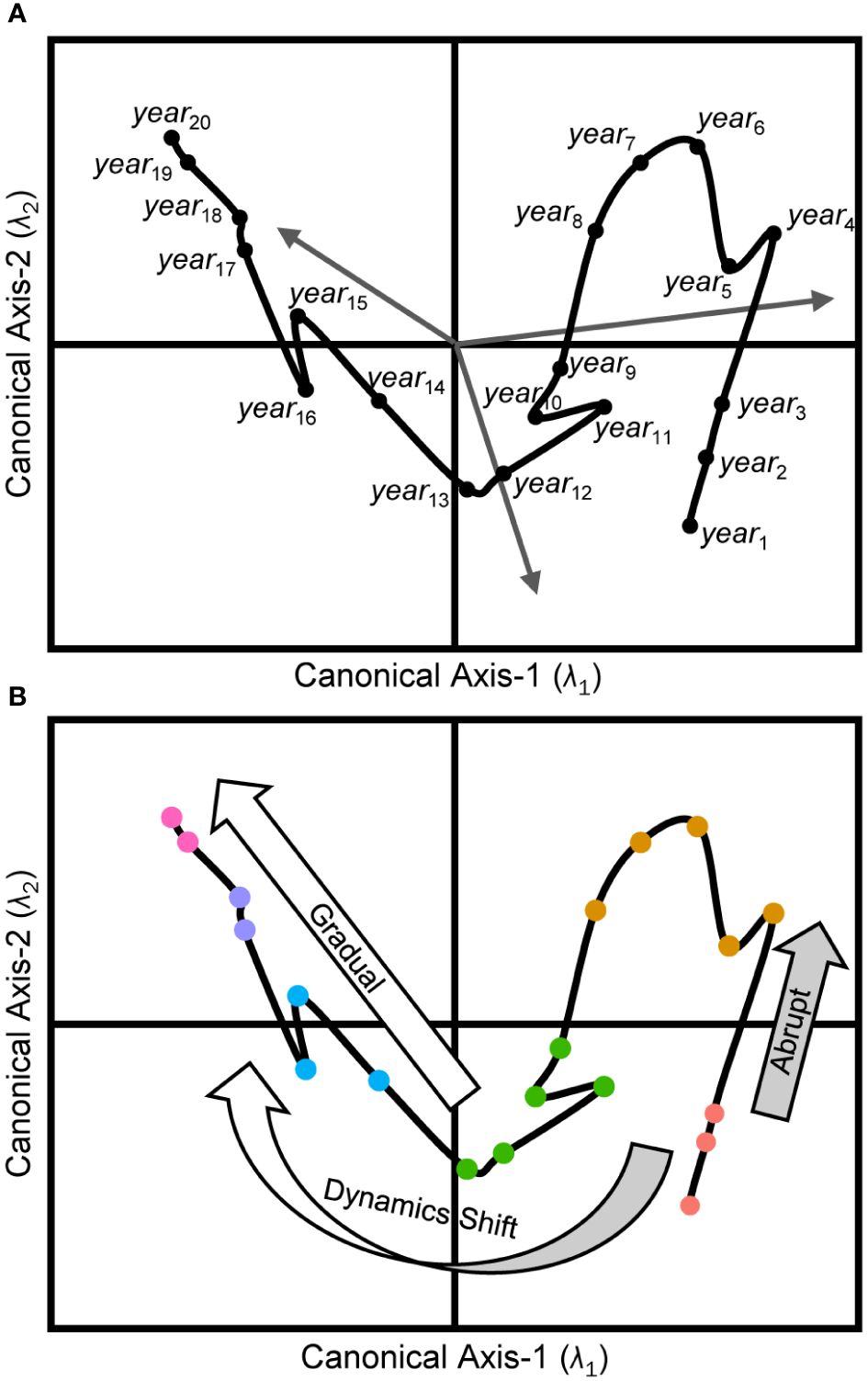
Figure 1 Conceptual model of ecosystem trajectories. Panel (A) illustrates an RDA ordination diagram projecting each object (yeari) from a multivariable response data set (Y) into canonical space defined by the model. Placement of objects (black dots) is related to the Euclidean dissimilarities derived from the same suite of response descriptors. Sites’ proximities are indicative of their resemblance, with sites closer together being more alike. Each orthogonal canonical axis (λi) accounts for an explained proportion (R2) of the total variability in Y, and the hierarchy of these axes is always such that R2λ1 > R2λ2. The terminating coordinates for response vectors (gray arrows) along each axis capture each indicator’s correlation with the model’s canonical axes’ scores. The ecosystem trajectory (black line) captures the chronological changes to the configuration of the underlying responses defining the system. Panel (B) depicts the classification of regime states (colored circles) for the same objects along the ecosystem trajectory. Large arrows align with abrupt (light gray arrow) and gradual (white arrow) transitions of the ecosystem trajectory as it evolves over short and long timescales, respectively. The curved bicolor arrow illustrates an example of a paradigm shift in the controlling organizational dynamics, ultimately resulting in the system trajectory trending in a completely new direction than previously observed.
In natural systems, ecosystem trajectories often exhibit characteristic behaviors in multidimensional subspaces (Lamothe et al., 2019) and it is valuable for managers and stakeholders to attempt to relate these behaviors to any known or hypothesized system-wide drivers or pressures (i.e., predictors). The classical analogy of the ball-and-cup is often used to illustrate the theory of ecosystem trajectories in a dynamical systems context and the reader is directed to Beisner et al. (2003) or Lamothe et al. (2019) for excellent reviews on the topic. In the analogy, consider an ecosystem’s status at any point in time – its ecosystem state – is defined by the specific arrangement of the response indicators selected to describe it (Figure 1A). This state is conceptualized as the instantaneous position of a ball traversing along an uneven three-dimensional surface. The shape of the surface represents the confluence of dynamic forcing conditions throughout the ecosystem at that moment as defined by observations from the representative suite of predictor indicators. The ball’s movement signifies an organizational change in the response resources, catalyzed by the surface’s variability over time.
The speed of ecosystem state changes is directly related to the topology of the surface, and apparent response-state stability is achieved when the immediate local surface is flat or the adjacent areas are too steep to be traversed (i.e., stable predictor conditions). In the natural environment, predictor surfaces continuously vary due to the dynamic nature of ecosystems and their constituent parts and this constant flux results in alterations to the shapes, heights, and slopes of the surface’s emergent features. These changes can deepen troughs, elevate hills, or make inclines and declines steeper or flatter. Consequently, the fluidity of the surface’s features creates natural temporal pathways (i.e., ecosystem trajectories) that guide the system state represented by the ball into wells or valleys that it cannot escape from and leading to a relative stable state.
As a predictor surface evolves, once seemingly insurmountable barriers may gradually (or quickly) ease until a tipping point is reached and, at this juncture, the new surface topology permits the ball to move away from its local equilibrium, ultimately resulting in an ecosystem regime shift once the ball settles into its new relative stable position on the surface. If the conditions or mechanism causing the tipping point and regime shift diminish, the system state may revert to its previous equilibrium position simply by reversing its path (recovery). However, if the predictor surface conditions transition through previously unobserved configurations, the recovery trajectory might follow a distinct and less predictable route back to its prior state, a phenomenon known as hysteresis. Alternatively, as the dynamic conditions of the surface continue to evolve it may settle into a wholly different equilibrium altogether, either temporarily (unstable state) or indefinitely (alternative stable state).
In addition to noting the directionality of regime shift trajectories, it is crucial to consider the temporal scale of significant changes (Figure 1B). These changes can occur rapidly, in saltatory shifts (Lamothe et al., 2017, 2019) across months or years, and possibly caused by pulsed or catastrophic disturbances. For example, in fisheries management, rapid regime shifts in stocks can be triggered by overfishing or abrupt changes in environmental conditions (Powell and Xu, 2011; Mollmann and Diekmann, 2012), leading to sudden declines in fish populations. Conversely, they may display gradual shifts (Lamothe et al., 2017, 2019) over many years to generations, typically due to long-term, system-wide reorganizations. For instance, sustainable fisheries practices and conservation efforts may be implemented or updated over the course of decades and can lead to relatively slow, but notable, changes to fish stock levels and ecosystem health (Worm et al., 2009; Neubauer et al., 2013; Melnychuk et al., 2017). Understanding which temporal scales are germane to a specific ecosystem is essential for implementing effective management strategies over the long term.
Within the realm of ecosystem-based fisheries management (EBFM), understanding the unique system-level dynamics within a given management unit can be advantageous to decision makers. Providing an accurate depiction of a fishery ecosystem’s historical trajectory assists resource managers in constructing a narrative detailing the relative changes to stocks’ sizes, health statuses, and productivities, and allows for correlating these changes to known natural, behavioral, and management intricacies. Evaluating critical trade-offs, historical dynamics, and shifting stable periods among resource pools and ecosystem sub-systems directly supports decision makers in prioritizing assets for management efforts. In particular, when combined with contemporary information related to the potential for notable predictor surface changes, this knowledge can guide both passive and active monitoring efforts, and enable the recursive adjustment of organizational goals and objectives to increase the effective implementation of an EBFM framework (Link, 2016a; Tommasi et al., 2017; Dell’Apa et al., 2020).
Furthermore, resource managers may stand to gain substantial benefits by categorizing segments of a fishery ecosystem’s trajectory as “alternate” or “unstable” equilibrium states. Regime state classification may also help identify early warning signs of an approaching tipping point, and creates reference markers to quantify the speed of state changes (or recoveries) for key fishery resources around these bifurcation points (Beisner et al., 2003; Deyoung et al., 2008; Scheffer et al., 2009; Lamothe et al., 2017). By developing tools tailored for these purposes, it might be possible to proactively prevent or mitigate future ecologically, economically, and socially destructive scenarios.
The aim of this study is to integrate existing time series data of fisheries-management related descriptors into multivariate models capturing the fishery ecosystem’s responses over time in relation to its economically important upper- and lower-trophic-level resources’ population statuses, stock structures, and associated revenue trends. These models will be utilized to document the fishery response trajectory in a large marine ecosystem (LME). They will also enable a direct evaluation of the connections between fishery regime state changes and/or tipping points, and a range of predictors encompassing basin- and regional-scale climatology, alterations in artificial and natural habitats, variability in water quality, and other anthropogenic drivers and pressures specific to the study LME. Ultimately, this research seeks to establish a framework for conducting comprehensive assessments of fishery ecosystems at a regional scale within an EBFM paradigm, and to help natural resource managers avoid potentially disastrous shifts to important subsistence and economic resources.
2 Materials and methods
2.1 Study system
The Gulf of Mexico (GoM) large marine ecosystem is a semi-enclosed basin spanning approximately 1.5 million km2 (Kumpf et al., 1999). Its waters support diverse marine activities and economies in the southeastern United States, Mexico, and Cuba (Kildow et al., 2014, 2016; NMFS, 2018). Fishery resources in the U.S. portion of the GoM LME are managed by the Gulf of Mexico Fisheries Management Council (GMFMC), in accordance with the Magnuson Fishery Conservation and Management Act of 1976 (Hsu and Wilen, 1997; USDOC, 2007). The GMFMC comprises decision makers from bordering States, the National Oceanic and Atmospheric Administration (NOAA), the commercial and recreational fishing industries, and other local stakeholder and expert groups. Historically, the region faced significant commercial fishing pressures, first from international fleets and later from U.S. efforts (NRC, 1994; Karnauskas et al., 2015). Notably, effective biological catch limits for the area were realized only after the 1996 Congressional authorization of the Sustainable Fisheries Act, which amended the 1976 Fisheries Conservation and Management Act (Hsu and Wilen, 1997). Additionally of note, the GoM LME differs from many other U.S. LMEs in that its recreational fishing activities have a substantial impact on the population dynamics of exploited species, and elicit effects comparable to that of the commercial fishing fleets (Coleman et al., 2004).
Nationwide, United States’ federal fisheries managers have prioritized EBFM (Link, 2016b), and the integrated ecosystem assessment (IEA) implementation scheme (Levin et al., 2009) has gained popularity (Diekmann and Mollmann, 2010; Andrews et al., 2014). Like in other LMEs, NOAA hosts an active IEA program in the GoM (GoM IEA) that produces a semi-regular ecosystem status report (ESR) for the region. Generally, ESRs contain numerous time series of descriptors capturing trends in the status of the important living marine resources, physical-chemical conditions, and associated natural or anthropogenic components unique to their regions (NOAA, 2009; Karnauskas et al., 2013; Kelble et al., 2013; Andrews et al., 2014; Karnauskas et al., 2017a). Presently, the indicators generated by GoM IEA are not directly incorporated into fisheries management decision-making. In achieving the study objectives outlined here, these analyses provide a case study for operationalizing the GoM ESR data to quantitatively define the LME’s fishery ecosystem and its associated trajectory. This work will also serve as a useful framework for resource managers in other LME’s hoping to use their ESRs to do the same.
2.2 Data assembly
The data for this study were drawn from the 2017 GoM ESR (Karnauskas et al., 2017a) and encompassed the period 1986–2013. The 2017 ESR was produced by the GoM IEA office to update the first GoM ESR (Karnauskas et al., 2013), and the authors substantially refined the descriptor pool to reduce covariation, redundancy, and sensitivity, while also accounting for time series’ accessibility, reliability, and importance to the GoM LME (Karnauskas et al., 2017a). The data were parsed for this investigation according to a response-predictor framework (details below) such that the fishery ecosystem’s response trajectory could not only be described, but also tested against the various LME predictors thought to affect its underlying organizational dynamics (i.e., stable states, shifts, and tipping points).
2.2.1 Fishery ecosystem response characteristics
To conceptualize the GoM fishery ecosystem, a suite of response indicators (Y) was selected to account for the population statuses (in terms of stock size, structure, and/or function), multispecies community structure, and relative commercial value of the living marine resources in the region. Each of the 23 individual indicators selected (Table 1; Supplementary Figure S1) represents an annualized value for the state of a particular aquatic resource or ecosystem-level driver or pressure within the GoM LME.
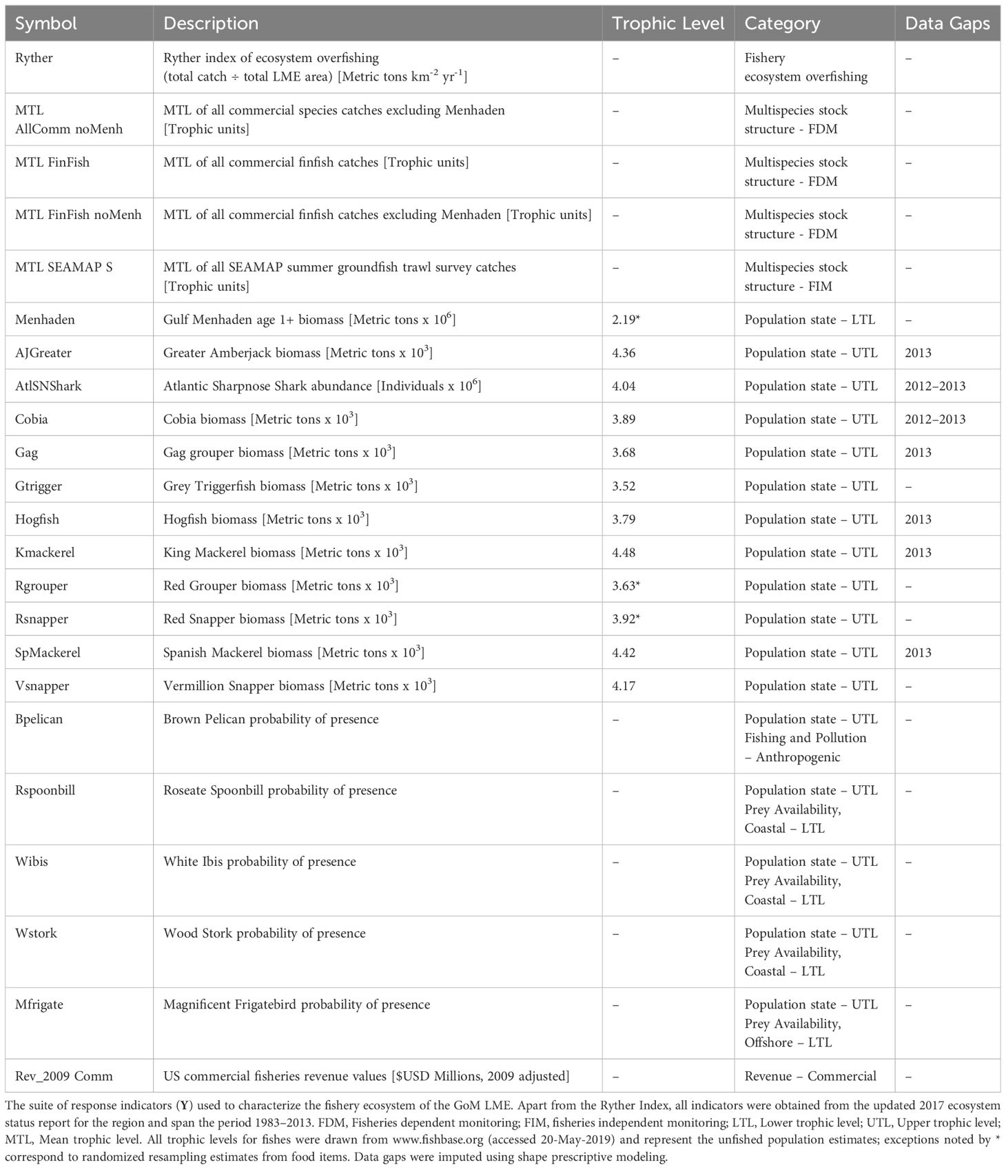
Table 1 Fishery ecosystem response indicators for the Gulf of Mexico (1986–2013).
2.2.1.1 Lower-trophic-level indicators
The majority of the population status indices were drawn from upper-trophic-level (UTL) species, and the only lower-trophic-level (LTL) response directly included here was the annual estimated biomass of age 1+ Gulf Menhaden (Brevoortia patronus). This single LTL indicator was used to describe the fishery ecosystem because the Menhaden fishery is the largest commercial fishery in the GoM (NMFS, 2023), a major dietary resource to various piscivorous species (Sagarese et al., 2016; Berenshtein et al., 2023), and an important ecological factor throughout the region (Olsen et al., 2014). Additionally, it was included in the 2017 ESR update as a leading indicator for the amount of forage biomass available within the LME (Karnauskas et al., 2017a). This important forage resource was ultimately retained in the response suite as opposed to the predictor suite not only due to its importance as a commercial fishery and managed species (Vaughan et al., 2007; SEDAR, 2018), but also to capture the direct impacts of anthropogenic and natural environmental variability in this important trophic link of the LME’s food web. Lastly, to retain this critical species for consideration in the characterization of fishery ecosystem trajectory it must be included in the response indicator suite.
2.2.1.2 Upper-trophic-level indicators
The UTL time series used in this study were primarily drawn from economically important fishes. Biomass estimates for 11 species managed by the GMFMC were selected for analysis (Table 1), but this selection was limited to only those 2017 ESR species with updated assessment estimates post-2010 (Karnauskas et al., 2017a). In addition, three fisheries dependent monitoring (FDM) indicators were investigated, representing the annual mean trophic level (MTL) of key subsets of fisheries targets. Including two for commercial catches of all finfish species (both with and without Gulf Menhaden), and one for commercial catches of all vertebrate and invertebrate species harvested (excluding Gulf Menhaden). Changes in MTL can often be interpreted as structural changes (e.g., size at age distributions, catch compositions) to the underlying populations due to fishing activities, and with decreasing MTLs often seen as a sign of unsustainable practices (Pauly et al., 1998; Essington et al., 2006; Branch et al., 2010). The MTL of catches from an annual summer groundfish trawl survey was also included as the sole fisheries independent monitoring (FIM) indicator for multispecies stock structure. The MTL values estimated by FIM, when compared against corresponding FDM values, can highlight potential disconnects between what is available in the fisheries ecosystem, versus what is extracted by the commercial fishing industry, respectively (Karnauskas et al., 2017a).
2.2.1.3 Mixed-trophic-level indicators
Three waterfowl species (Table 1), Roseate Spoonbill (Platalea ajaja), White Ibis (Eudocimus albus), and Wood Stork (Mycteria americana), were included due to the current reliance by resource managers on these species as indicators representing changes to aquatic prey abundance in coastal areas (Stolen et al., 2005; Ogden et al., 2014; Karnauskas et al., 2017a). Two additional waterbirds, Brown Pelican (Pelecanus occidentalis) and the Magnificent Frigatebird (Fregata magnificens), were also included due to their shared open water foraging behavior. Additionally, the Brown Pelican is readily impacted by human fishing and pollution, making it a valuable short-term indicator of the ecological stressors affecting nearshore marine environments. In contrast, the Magnificent Frigatebird serves as a robust long-term indicator of the health and biological capacity of coastal adjacent areas due to its relatively slow reproductive rate (Karnauskas et al., 2017a).
2.2.1.4 Fishery revenue and sustainability indicators
The final two response indicators included in this fishery ecosystem analysis were related to socio-economic aspects of the GoM LME. Firstly, to gauge the overall economic impact of large-scale commercial fisheries, the total U.S. GoM commercial fisheries revenues adjusted to 2009 U.S. dollars (Karnauskas et al., 2017a) were retained. Secondly, the Ryther index, a standardized metric of total annual fisheries removals distributed across space (t km-2 yr-1), was included as a means to monitor ecosystem overfishing (Link and Watson, 2019). It is worth noting that the Ryther index is the only indicator not sourced from the 2017 GoM ESR.
2.2.2 Factors influencing fishery ecosystem responses
The suite of predictor indicators (X) hypothesized to affect the overall fisheries ecosystem response, and subsequent trajectory, comprised 15 time series (Table 2; Supplementary Figure S2) representing artificial habitat availability, human development and resource exploitation patterns, large-scale climatic trends, and aquatic physical-chemical conditions. Unfortunately, given the effort to minimize data redundancy and covariation in the 2017 GoM ESR, the pool of predictor indicators to draw from was considerably smaller compared to previous ecosystem-level analyses based on the 2013 report (Karnauskas et al., 2015; Kilborn et al., 2018). Nevertheless, the selected descriptors were indicative of many major processes and drivers essential to the GoM LME, its fisheries, and other living marine resources (Karnauskas et al., 2015; Karnauskas et al., 2017a; Kilborn et al., 2018).
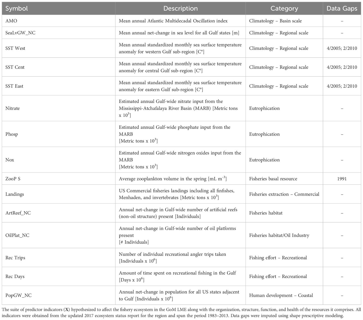
Table 2 Fishery ecosystem predictor indicators for the Gulf of Mexico (1986 to 2013).
2.2.2.1 Artificial habitats, energy infrastructure, and human population growth
As elsewhere, submerged artificial structures in the GoM LME have been demonstrated to be influential habitats for marine life (Paxton et al., 2020a, b; Gardner et al., 2022). In the GoM there exists a distinction between features related to industrial crude oil and gas development (i.e., drilling apparatuses, oil platforms) and other features like shipwrecks and concrete debris that are unrelated to these activities (Karnauskas et al., 2017a; Gardner et al., 2022). For this study two indicators were retained from the 2017 ESR representing the annual net-change in known artificial habitats allocated across the two aforementioned types (i.e., industrial, non-industrial). Oil and gas industry activity may also be interpreted as a human development index and/or a proxy for the ecosystem-wide potential for environmental contamination due to infrastructure failures, operation, or decommissioning (Cordes et al., 2016; MacIntosh et al., 2022). Another explicit anthropogenic indicator investigated was the annual net-change in the populations of the Gulf States’ coastal watershed counties, aggregated over the entire region for the study period.
2.2.2.2 Fisheries sector utilization
Utilization of fisheries resources across the commercial and recreational sectors was measured in terms of landings and effort, respectively. For the commercial fishing industry, a Gulf-wide measure of the biomass landed for all commercial catches (all finfish incl. Menhaden + invertebrates) was used to estimate total extractions. Recreational fishing pressures were estimated in terms of effort in the 2017 GoM ESR (Karnauskas et al., 2017a), partially because recreational anglers value opportunity and quality of the fishing experience as well as the magnitude of individual catches (Moeller and Engelken, 1972; Holland and Ditton, 1992), and this sector is less fundamentally constrained by economics. Thus, recreational fishing effort was recorded by the number of angler days utilized per year and the total annual number of individual trips taken.
2.2.2.3 Climatological and temperature indicators
This study incorporated four large-scale indicators of sea surface temperature (SST) related to global climate trends. Specifically, three descriptors directly accounted for mean annual SST anomalies across three distinct sub-regions within the GoM LME – the western, central, and eastern regions – while the fourth served as a proxy for temperature changes in the northern Atlantic basin, the Atlantic Multidecadal Oscillation (AMO) (Schlesinger and Ramankutty, 1994).
Alone, SST is a well-known factor influencing fishes, with species (and even different life stages within a species) exhibiting varying tolerances to temperature (Pauly, 1980; Helfman et al., 2009). The regional SST indicators used here aimed to identify any large-scale spatial considerations within this metric. Conversely, AMO is associated with a variety of teleconnected processes that vary depending on geographic location (Nye et al., 2014). Recent research within the GoM LME suggests that the warm phase of the AMO coincides with decreased total nitrogen loading from the Mississippi-Atchafalaya river basin (MARB), increased terrestrial fertilizers, elevated Gulf-wide SST, and higher levels of seasonal hypoxia offshore Louisiana and Texas (Kilborn et al., 2018). Additionally, the AMO index has shown strong correspondence with regional fisheries trends over time, although the mechanistic reasons for this relationship remain unclear (Karnauskas et al., 2015; Kilborn et al., 2018).
2.2.2.4 Physiochemical and water quality indicators
The remaining physiochemical indicators investigated here focused on system-wide eutrophication due to nutrients discharged from the MARB, specifically, nitrate, nitrogen oxides, and phosphorus. These eutrophication metrics also serve as proxies for terrestrial agriculture and fertilizer use within the MARB (Karnauskas et al., 2017a), making them potential human development indicators if desired. The final measure of water quality included in this study was the average volume of zooplankton estimated for the annual springtime bloom. This descriptor captures an important LTL prey resource for many species that can affect their perception of “high-quality” habitat and, thus, may dramatically impact their distributions and abundances (Cushing, 1975; Grimes and Finucane, 1991; Boldt et al., 2019).
2.2.3 Synthetic temporal indicators
Lastly, to explicitly account for temporal variability in the organization of resources and the trajectory of the GoM fishery ecosystem, a series of synthetic predictors (T) were generated using asymmetric eigenvector mapping (AEM) (Blanchet et al., 2008b, 2011). Via this method, the regular, annual-interval time-series spanning 1986–2013 was decomposed into a set of periodic eigenfunctions encompassing all temporal correlation scales and frequencies within the 28-year period (Supplementary Figure S3). These predictors were then employed in subsequent variable selection routines and canonical analyses to gain insights into the temporal determinants of the fishery ecosystem’s trajectory, stable states, and shifts. Thus, this approach helps enable the identification of future tipping points and shifts by modeling historical patterns in resources’ responses as they relate to the explicit scales of variability represented by the selected AEMs (Angeler et al., 2013; Legendre and Gauthier, 2014; Baho et al., 2015).
2.3 Statistical analyses
2.3.1 Data pretreatment
All response and predictor data tables were configured to contain annualized observations (rows) for each descriptor (columns) described above. Note that the numerical methods utilized in these analyses do not permit missing observations within an indicator (Legendre and Legendre, 2012). Therefore, any missing values identified in Tables 1, 2 were imputed using shape prescriptive modeling via the ‘SLM-shape language modeling’ toolbox for MATLAB (D’Errico, 2009), a form of interpolation based on least squares splines (Supplementary Figure S4). No indicator’s time series contained more than two missing observations. However, seven of 11 response fishes were missing the final values in the series, and with two of those also lacking the penultimate value. Due to this, interpretations of results during that specific two-year period should be approached cautiously for most fishes.
All non-synthetic data (Y, X) were centered and standardized using z-scores translation (Legendre and Legendre, 2012). In constrained analyses where only synthetic variables served as predictors, temporal variables remained untransformed. In analyses combining both eigenfunctions and ESR predictors for direct comparisons against the fishery ecosystem’s responses, temporal variables were z-score standardized alongside the ESR variables. Resemblance between pairs of multivariate objects within all descriptor categories were calculated using Euclidean dissimilarities (Faith et al., 1987; Legendre and Legendre, 2012).
2.3.2 Multivariate modeling
All modeling exercises were implemented using MATLAB R2020a (MATLAB, 2020) in conjunction with the Darkside (Kilborn, 2020) and Fathom (Jones, 2017) toolboxes for numerical ecology. Visualizations were created using both MATLAB and the package ‘ggplot2’ (Wickham, 2016) implemented in R (R Core Team, 2022).
The 2017 GoM ESR data were primarily analyzed two ways. First, an explicit temporal model was constructed to account for relevant periodic timescales across the sampling period and, ultimately, to define the fishery ecosystem trajectory (Supplementary Figure S5). This approach starts by identifying which temporal factors (i.e., AEMs) best explained the fishery resources’ variability within the GoM LME and then seeks to assess which environmental predictors also relate to the temporally constrained response trajectory. The fishery ecosystem trajectory model is also used for pinpointing when significant changes occurred in the controlling dynamics of the response system. Secondly, clustering exercises were utilized to identify apparent-stable states within the GoM LME’s fishery ecosystem from 1986–2013 and then relate them to the fishery ecosystem trajectory (Supplementary Figure S6). Discriminant analyses were employed to characterize the differences among regimes. Finally, a system-wide synthesis was created to align the fishery ecosystem’s trajectory with the observed dynamical-system characteristics, providing EBFM context for monitoring future ecosystem state shifts.
2.3.2.1 Ecosystem trajectory modeling
The time series spanning 1986–2013 was decomposed into its component AEMs (Supplementary Figure S3). Those AEMs with positive eigenvalues (i.e., positive temporal autocorrelation) were assembled into the temporal predictor matrix (T) and subjected to forward variable-selection with RDA against the standardized response matrix (Y). Following the recommendation of Blanchet et al. (2008a) to minimize type-I error in subsequent variable selection procedures, the global model of Y against T (RDAY|T) was initially tested (α = 0.05 and 104 permutations) before conditional tests were applied. Forward selection was performed by maximizing the partial F-statistic (Miller, 1975; ter Braak and Smilauer, 2002), and significance was determined using randomization methods (Legendre and Legendre, 2012) with the same criteria as the global model. The selection process continued until no new descriptor additions either significantly affected the model or produced a candidate model whose adjusted coefficient of determination (R2adj; Ezekiel, 1930) exceeded that of the global model (Blanchet et al., 2008a). The optimal subset of eigenvectors retained after variable selection (T*) was used to create the final temporal model (RDAY|T*) for the fishery ecosystem’s response, constrained by the periodic timescales deemed most appropriate for the GoM LME.
Subsequently, the fitted axis scores of the first two canonical axes (λi, where i = [1,2]) of the temporal model were independently subjected to a second round of variable selection. This time, stepwise-RDA coupled with Akaike’s (Akaike, 1974) information criterion (AIC) was used to determine the most parsimonious suite of ecosystem predictors (X*) that best accounted for the time-constrained model’s predicted responses. A similar selection process was also applied to the residual values from the temporal model (i.e., the non-temporal fishery ecosystem response) to determine if any of the ESR predictors could account for this aspect of the variability in the fishery ecosystem.
Multivariate ordinations, produced via RDA, captured the relative similarity among years with respect to the suites of descriptors characterizing the fishery response, and the temporal autocorrelation structures and selected ESR predictors used to constrain it. The subsets of AEM and ESR predictors (T* and X*, respectively) were also used in a variation partitioning analysis (Borcard et al., 1992; Peres-Neto et al., 2006) against Y. This analysis enabled formal quantification of the total variability in the GoM LME’s fisheries ecosystem response (Y) and its decomposition into four specific partitions: purely temporal factors (TP), temporally organized LME components (XT), non-temporally structured LME components (XnT), and unexplained response variability (ε) not accounted for by any of the predictors investigated.
The elucidation of relative changes in the controlling dynamics of the fishery ecosystem trajectory will be achieved through examining a novel visualization of the canonical axes (λi) from the temporal model. Specifically, plotting the temporal RDA model’s first two fitted axes (λ1 and λ2) as a function of year on the same figure can provide insights into whether their underlying correlation structures are working in tandem (resulting in relatively parallel axes’ scores over time), or independently (leading to divergent or convergent slopes). Any point in time where the axes’ scores intersect marks a substantial paradigm shift in the organizational controls of the fishery ecosystem’s response. When analyzed in conjunction with the fishery ecosystem’s regime states, the timing of an intersection can be instrumental in identifying previous ecosystem-level control shifts. Furthermore, continuous monitoring and annual production of these plots may help predict future regime shifts or potentially serve as an early warning indicator.
2.3.2.2 Fishery ecosystem regime states and shifts
To fully characterize the theoretical response trajectory for the GoM’s fishery ecosystem, detailed descriptions are essential. First, the multivariate regime states within the response data (Y) were identified using the unweighted pair group method with arithmetic mean (UPGMA; Rohlf, 1963) combined with dissimilarity resemblance profiles as clustering decision criteria (Clarke et al., 2008; Kilborn et al., 2017), a method referred to as DISPROF clustering hereafter. During DISPROF clustering, a hypothesis test was conducted for each node of the UPGMA connection-tree to determine if there was “multivariate structure” among the observations grouped within the branch defined by that node. This test was repeated for all branches in a clustering solution, examining multivariate structure at the largest (all objects) and smallest (two objects) subsets of observations grouped by UPGMA. The progressive Holms p-value correction method was used (Clarke et al., 2008; Legendre and Legendre, 2012) and significance for each cluster was determined using α = 0.05 and was based upon 104 permutations of the raw data.
To explore the relative differences across regime states identified via DISPROF clustering, a canonical analysis of principal coordinates (CAP; Anderson and Willis, 2003) was used. This method, while similar to RDA, aims to generate orthogonal ordination axes that maximize the among-group variability (here, based on the clustering solution) rather than total variability among all objects, as in RDA. In addition to the group-specific ordination, the CAP procedure also produces a leave-one-out cross-validation (LOO-CV) that provides valuable insights into the model’s ability to reclassify unknown samples and helps identify which groups were most frequently confused with one another. This information is also useful for assessing whether regimes are relatively stable (i.e., low misclassification rates), or if they represent periods of instability between stable periods, thus displaying higher misclassification rates across adjacent regimes in the time series.
To assess the system-wide stability of the GoM LME’s fishery ecosystem, a comprehensive approach was utilized. A visual assessment of the fishery ecosystem trajectory depicted in the ordination space of RDAY|[ X* T* ] was coupled with “lag-plots” (Lamothe et al., 2019) of all annual Euclidean distances (YEUC). Lag-plots visualize the pairwise dissimilarities as a function of the time lags within the time series relative to the initial year (ranging from 0 to 27 years). Lag-plots also incorporate a line depicting the observed distance from the baseline year (1986) for each consecutive year in the model, and this feature is developed using a five-year moving average of the distances (Lamothe et al., 2019). This allows for a depiction of the relative magnitude of changes to the fishery ecosystem over the study period and among individual years or regimes, as well as the variability within them.
The general shape of the smoothed lag-plot’s distance-to-baseline vs. time-lag curve offers valuable insights into the resilience and stability of the dynamical system over time (Lamothe et al., 2017, 2019). This graphical representation allows for determination of whether the fishery ecosystem has experienced persistent directional changes (indicated by a monotonic and increasing slope), responded to a disturbance or dynamics shift but then displayed recovery – either with or without hysteresis (displaying a parabolic curve), or shows no apparent changes over time (a flat slope). A fourth lag-plot scenario captures a system responding to an initial perturbation via directional changes and movement of the ecosystem state away from the baseline (increasing slope), followed by a period that appears to show signs of recovery (displaying a change in slope direction or flattening), and then the system ultimately continues its evolution while maintaining substantial distances from the baseline configuration (indicated by a return to an increasing slope). This particular pattern is denoted the “Humpty Dumpty” form (Lamothe et al., 2019) and is often characterized by a shift in the lag-plot’s concavity at an inflection point associated with a particular time lag relative to the baseline year.
3 Results
3.1 Fishery ecosystem trajectory modeling
The regular annual time series spanning 1986–2013 was decomposed into 27 temporal AEM indicators (Supplementary Figure S3). Among these, 14 modeled positive temporal autocorrelation periods (T) and, following forward-selection of T against Y, the optimal temporal model of the GoM LME’s fishery ecosystem response included only the first six of these AEMs (T*; Figure 2). The RDAY|T* model effectively captured approximately 76% of the adjusted total variability in Y (R2 = 0.8139, R2adj = 0.7608) with a high level of significance (F = 15.31, p = 0.0001, dfmodel = 6, dferror = 21), while relying solely on synthetic AEM predictors (Supplementary Table S1).
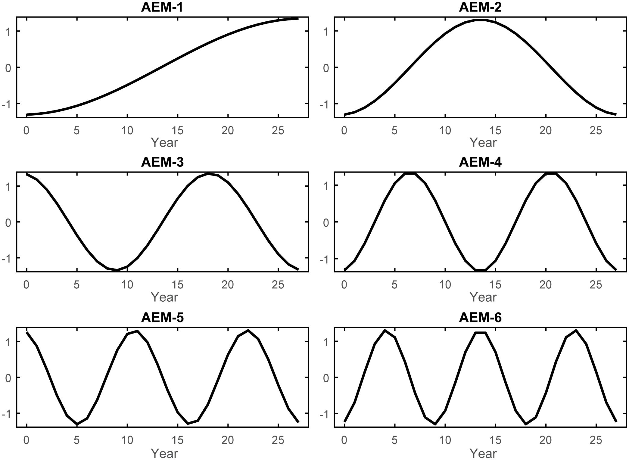
Figure 2 Selected asymmetric eigenvector maps. The six AEM autocorrelation structures retained by forward variable selection to describe the variability in the GoM fishery ecosystem response (Y). AEMs were produced via eigenvector decomposition of the regular annual time series spanning 1986–2013 and then used to develop an optimal temporal model of LME’s living marine resources’ variability throughout the study. As i increases in the AEM-i label, so does the frequency of the periodic function, and ultimately the temporal trend being modeled across the 28-year period.
The first two canonical axes (λ1 and λ2) represented about 66% of the unadjusted variability in Y (Table 3). Among the six AEMs included in T*, the first two temporal predictors were the most capable of modeling these two axes (Supplementary Table S1, Supplementary Table S2) and accounted for trends spanning 28 and 14 years, respectively (Figure 2). When the values for λ1 and λ2 were plotted as functions of time (Figure 3), a notable pattern emerged. The period 1986–1994 shows two rapidly convergent lines that ultimately intersected around 1994, after which they continued with downward sloping trends that were largely parallel over the remainder of the time series. This distinct activity highlights significant alterations to the fishery ecosystem’s behavior during the study period with an inflection point between 1994/1995.
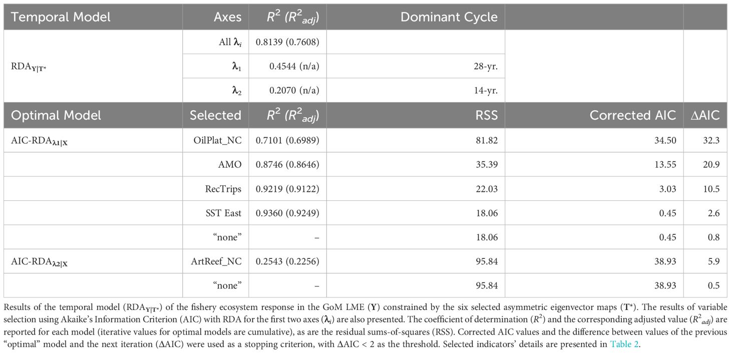
Table 3 Temporal model and variable selection results for the Gulf of Mexico fishery ecosystem (1986–2013).
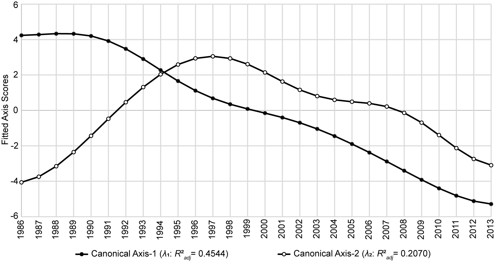
Figure 3 Temporal controls of Gulf of Mexico fishery ecosystem (1986–2013). Fitted site scores from the first two canonical axes (λ1 and λ2) of the GoM fishery ecosystem’s temporal model (RDAY|T*) plotted as a function of time. Fitted scores correspond to the final model’s prediction for each year’s position in canonical space given the observed data. Axes’ R2adj values describe the proportion of the total variability in the fishery ecosystem response accounted for by each.
Variable selection (Table 3) using RDA with AIC for λ1 and λ2 against X yielded four ecosystem-level predictors that best explained λ1: net-change in oil platforms, AMO index, recreational fishing trips, and SST in the eastern region. Additionally, one predictor, net-change in non-industrial artificial reef structures, was selected to account for λ2. Interestingly, no X variables were selected to account for the residual variability (~24%) remaining in the temporal model (i.e., non-temporally structured response). The integrated RDA model of Y against the combined [X* T*] matrix demonstrated only a slight improvement over RDAY|T* while still providing a high-quality fit (R2 = 0.8696, R2adj = 0.7799) and significant model (F = 9.70, p = 0.0001, dfmodel = 11, dferror = 16) for the variability in Y. Similarly, though, the first two canonical axes accounted for ~66% of the GoM fishery ecosystem’s response over time (Figure 4).
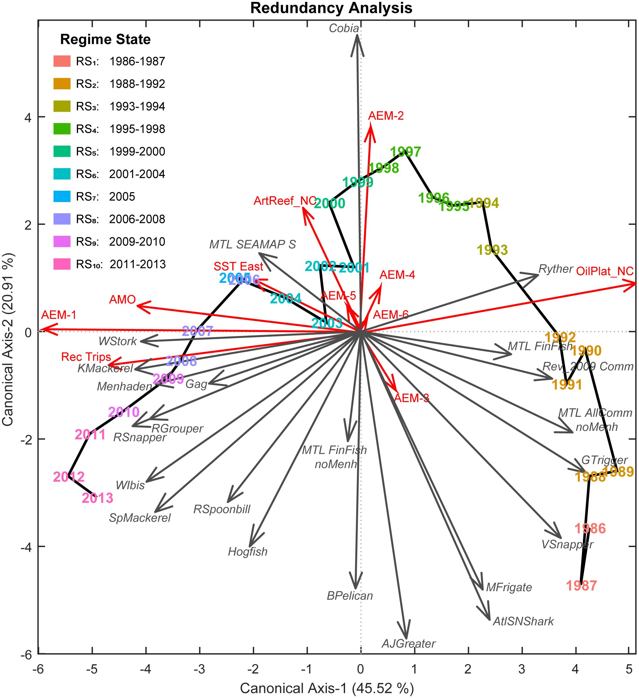
Figure 4 Fishery ecosystem trajectory for the Gulf of Mexico (1986–2013). Ordination diagram for the final GoM fishery ecosystem model (RDAY|[X* T*]) constraining the regional living marine resources’ responses (Y, gray arrows, italic labels) by the indicators retained from the ecosystem status report (X*, red arrows) and the selected temporal autocorrelation functions (T*, red arrows) spanning 1986–2013. Interpretation of this diagram closely follows the description in the conceptual model presented in Figure 1, but with the addition of predictor vectors. In this context, the visualization captures the relationships between the response and predictor indicators along with their contributions to the underlying resemblance among years and, ultimately, the placement of those objects in multivariate ordination space. As with the response vectors (gray arrows), predictor vectors’ endpoints are based upon their correlations with the two canonical axes (λi) derived by the model. Proximities are indicative of resemblance, with years closer together being more alike, and each new axis accounts for a decreasing proportion (R2) of the total explained variability in the fishery ecosystem response (Y). The solid black line connects years chronologically and depicts the fishery ecosystem trajectory. Regime state (RSi) membership was determined via DISPROF clustering of Y and is denoted in a legend as well as by color. Colors for regimes are preserved in subsequent figures for clarity.
The variation partitioning analysis (Table 4) revealed that the organization of living marine resources in the GoM LME was significantly influenced by temporal factors, particularly the temporally structured ESR predictors in X* (fraction XT = 0.4815) and the unassociated, purely temporal components in T* (TP = 0.2793). However, a substantial proportion of the total variability in the fishery ecosystem response remained unexplained (ε = 0.2201), indicating that none of the hypothesized predictors, temporal or otherwise, were able to capture this portion of the system-wide response.

Table 4 Variation partitioning results for the Gulf of Mexico fishery ecosystem (1986–2013).
3.2 Fishery ecosystem regime states, shifts, and lag-plot
The DISPROF clustering routine (Supplementary Table S3) successfully identified 10 distinct fishery ecosystem regime states (RSi) for the GoM LME from 1986 to 2013 (Table 5). The two-dimensional RDA ordination diagram (Figure 4) depicts the historical trajectory of the ecosystem as it transitioned through these relative stable states. Notably, half of the regime states (RS1, RS3, RS5, RS9) spanned no more than two years, and the year 2005 was the only year to cluster independently. Among the remaining regimes, two comprised three years (RS8, RS10), two others consisted of four years (RS4, RS6), and only one extended across a five-year period (RS2).
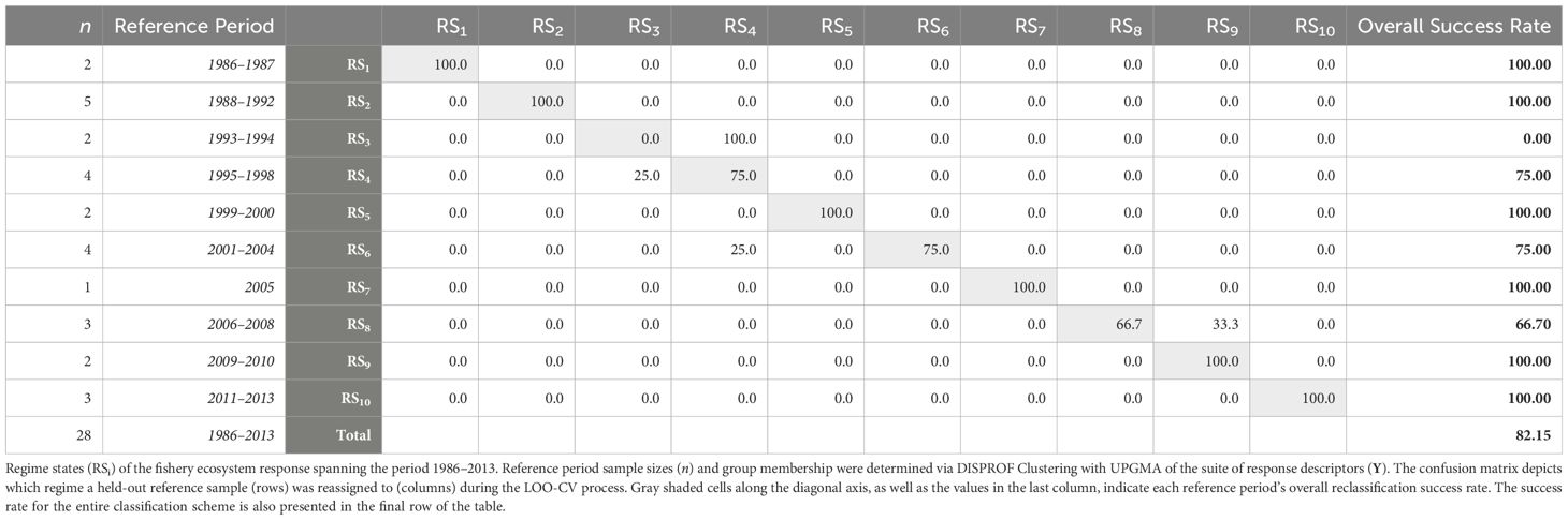
Table 5 Fishery regime state membership and leave-one-out cross-validation for the Gulf of Mexico fishery ecosystem (1986–2013).
The CAP ordination diagram for the fishery ecosystem response, while technically more appropriate for visualizing differences among groups, did not obtain appreciably different results than those produced via RDA (Supplementary Figure S7). Thus, only the RDA ordinations are discussed to highlight differences among all years as well as across regime states. The LOO-CV results (Table 5) for the CAP model of Y constrained by the DISPROF clusters (Supplementary Table S4) demonstrated an overall classification success rate of 82% and with RS1, RS2, RS5, RS7, RS9, and RS10 having 100% individual success rates. Interestingly, RS3, which had a 100% failure rate, was consistently reclassified as RS4 100%. Further, while RS4 had a 75% success rate, its failed classifications were all regularly reassigned to RS3, indicating a substantial overlap in the fishery ecosystem response state configurations between these two regimes, and possibly representing a transition period. Lastly, RS6 was reclassified as RS4 in 25% of cases, marking the only misclassifications involving non-adjacent regimes; RS8 was misclassified one-third of the time into RS9.
The smoothed lag-plot (Figure 5) displayed a consistent increase in distance from the baseline year until an initial peak in 1998. After this peak there is a slight dip in the trajectory through the early 2000s, which is succeeded by another mostly constant increase after 2002 and continuing through the remainder of the time series. Further, this observation also aligns with the relatively parabolic shape of the ecosystem trajectory projected into multivariate ordination space (Figure 4). Notably, the distributions of individual distances about the smoothed line at each time lag (Figure 5) did not display any notable outliers (i.e., saltatory changes). When considered holistically, the ecological implication is that from the start of the study period this fishery ecosystem’s resources demonstrated gradual directional changes away from their baseline state, then drastically responded to new controlling dynamics by quickly reorganizing back toward the baseline over a short time period, but ultimately returned to their evolution away from the baseline without ever fully recovering to any previously observed fishery regime state. This trajectory appears most consistent with the Humpty Dumpty model of ecosystem change (Lamothe et al., 2019).
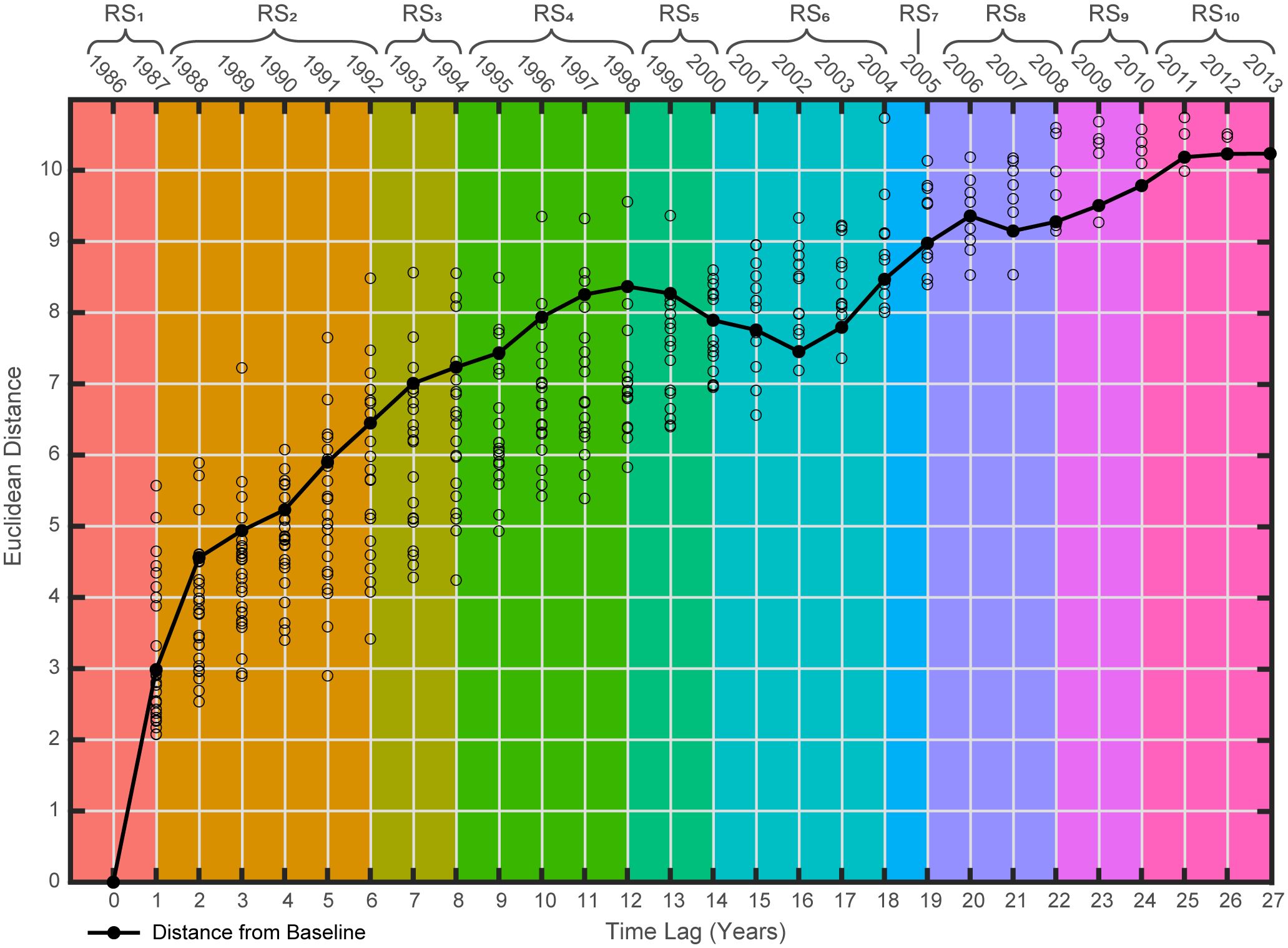
Figure 5 Smoothed lag-plot for the Gulf of Mexico fishery ecosystem (1986–2013). Pairwise Euclidean distances (circles) between all pairs of years in the suite of fishery response data (Y) plotted as a function of time-lags relative to the first year of the study (i.e., baseline). Each year’s observed distance to baseline (black line, filled-in circles) is plotted to visualize the total relative changes to the system’s resources and their organization. Regime states (RSi) identified via DISPROF clustering of Y are denoted at the top of the figure where the colors correspond to the RSi noted within the associated brackets and match those used in the previous ordination and subsequent figures.
4 Discussion
4.1 Gulf of Mexico fishery ecosystem’s trends, trajectory, and tipping point
In terms of managing fisheries resources in the GoM LME, these findings underscore two prominent timescales governing the system’s response to external forcing between 1986 and 2013: the 28-year and 14-year cycles. The long-period cycle was modeled as a constant gradual increase over time, reaching its peak toward the end of the time series (AEM-1; Figure 2). The shorter cycle was represented by a sinusoidal curve that increased until approximately 1999, followed by a mirrored decrease until the end of the study period (AEM-2; Figure 2). Greater variability (~45%) in the fishery ecosystem response (Figure 4) was explained by the long-term trend and the selected environmental descriptors captured by it (both positively and negatively). On the other hand, the 14-year cycle was associated with fewer system-wide responses and explained less variability (~21%), with only one ecosystem predictor linked to that cycle (Figure 4).
The alignment of the secondary temporal trend with the end of the first peak in the GoM fishery ecosystem’s smoothed lag-plot (Figure 5), which depicts the evolution of the system’s relative difference from the baseline year, is noteworthy. Primarily because the lag-plot’s initial rise to a peak, short-lived reversal in trend, and subsequent return to a gradual increase away from the baseline, best reflect a Humpty Dumpty ecosystem trajectory (Lamothe et al., 2019). In the case of the GoM LME, it appears that a change in the governing dynamics of the system became apparent in the response of living marine resources starting in the mid-to-late 1990s and settled into a new mode of control in the early 2000s (Figures 3, 5). This timing is also conspicuously coincident with the effective implementation of fishery regulations and annual catch limits in the region, due to the Sustainable Fisheries Act (Hsu and Wilen, 1997), as well as the negative-to-positive phase shift in the AMO index (Schlesinger and Ramankutty, 1994; Alexander et al., 2014).
Upon analysis of the trends depicted by the fitted canonical axes from the temporal model of the GoM fishery ecosystem’s response (Figure 3) a clear intersection is evident just after 1994, indicating a major tipping point after which the paradigm controlling the dynamics of the system’s response changed. Further, continuous growth in the fishery ecosystem’s dissimilarity relative to the baseline year (1986) until the end of RS4 (1998; Figure 5) suggests a lag of approximately five years between the tipping point and the observable response in the fishery resources that characterizes this new mode of control. Additionally, Figure 3 shows that in the five years preceding the 1994 shift in dynamics, the axes’ trend lines were clearly convergent, thus, displaying an early warning signal of the impending ecosystem-wide, paradigm shift in control of the living marine resources in the GoM LME.
4.2 Characterizing the Gulf of Mexico fishery ecosystem’s response dynamics
4.2.1 Managed fishes and the upper trophic level
Over the long-term and closely following the 28-year trend (AEM-1), several UTL fishes displayed concurrent increases in their abundance estimates (Figure 6). These species, ranked in decreasing order of the strength of this positive relationship, include King Mackerel (Scomberomorus cavalla), Red Snapper (Lutjanus campechanus), Red Grouper (Epinephelus morio), Spanish Mackerel (S. maculatus), Gag (Mycteroperca microlepis), and Hogfish (Lachnolaimus maximus). While all six of these species displayed generally increasing biomass trends over time, the first three exhibited very strong positive responses to AEM-1, whereas the last three were also negatively related (Figure 4) to the 14-year cycle (AEM-2), indicating that their gains were likely due to more recent developments in the fishery ecosystem.
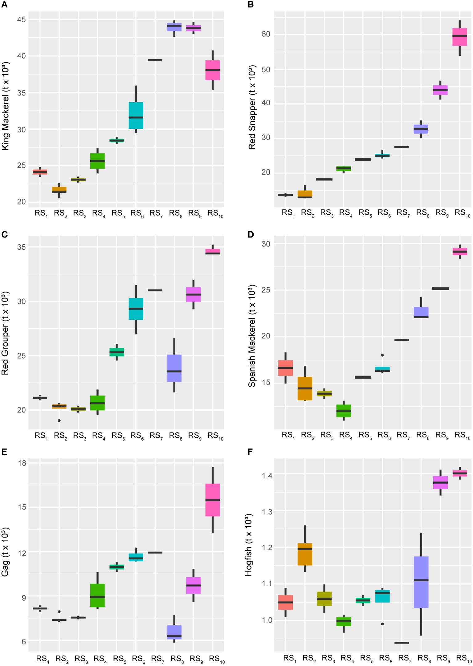
Figure 6 Boxplots across regimes for managed fishes displaying relative increases over time. Panels depicting boxplots for the raw data distributions of upper-trophic-level fishery resource indicators in the GoM LME spanning 1986-2013. Fishery response indicators (Y) for King Mackerel (A), Red Snapper (B), Red Grouper (C), Spanish Mackerel (D), Gag (E), and Hogfish (F) displayed relative increasing long-term trends over the study period. All species’ data represent biomass values. Colors correspond to the regime states (RSi) identified with DISPROF clustering of Y and match those used in previous figures and ordinations. Boxplots should be interpreted as follows: Horizontal lines depict the median value, and the lower and upper boundaries of each rectangle correspond to the 25th and 75th percentiles of the data, respectively. Whiskers extend to maxima and minima no more than 1.5x the inter-quartile range, and all other values are plotted as outliers (points). See Table 1 for indicator details and Table 5 for sample sizes.
Conversely, several species experienced long-term declines over the study period, including Gray Triggerfish (Balistes capriscus), Vermillion Snapper (Rhomboplites aurorubens), Atlantic Sharpnose Shark (Rhizoprionodon terraenovae), and Greater Amberjack (Seriola dumerili), all of which continued to persist at historically low levels (Figure 7). Among these, all were primarily negatively influenced by the 28-year trend (AEM-1) and showed significant reductions occurring in populations from the mid-1980s through the late 1990s (Figure 4). However, Greater Amberjack and Atlantic Sharpnose Shark, in particular, appeared to have experienced some form of population rebound following the 14-year cycle (AEM-2) and beginning around the turn of the century – although neither stock has returned to their historical highs. Cobia (Rachycentron canadum), on the other hand, was the only species apparently entirely driven by the 14-year trend (Figure 4), and they too are maintaining stock levels well below their historical highs. Notably, unlike many other species, Cobia reached their highest biomass levels in the late 1990s (Figures 6, 7; Supplementary Figure S1).
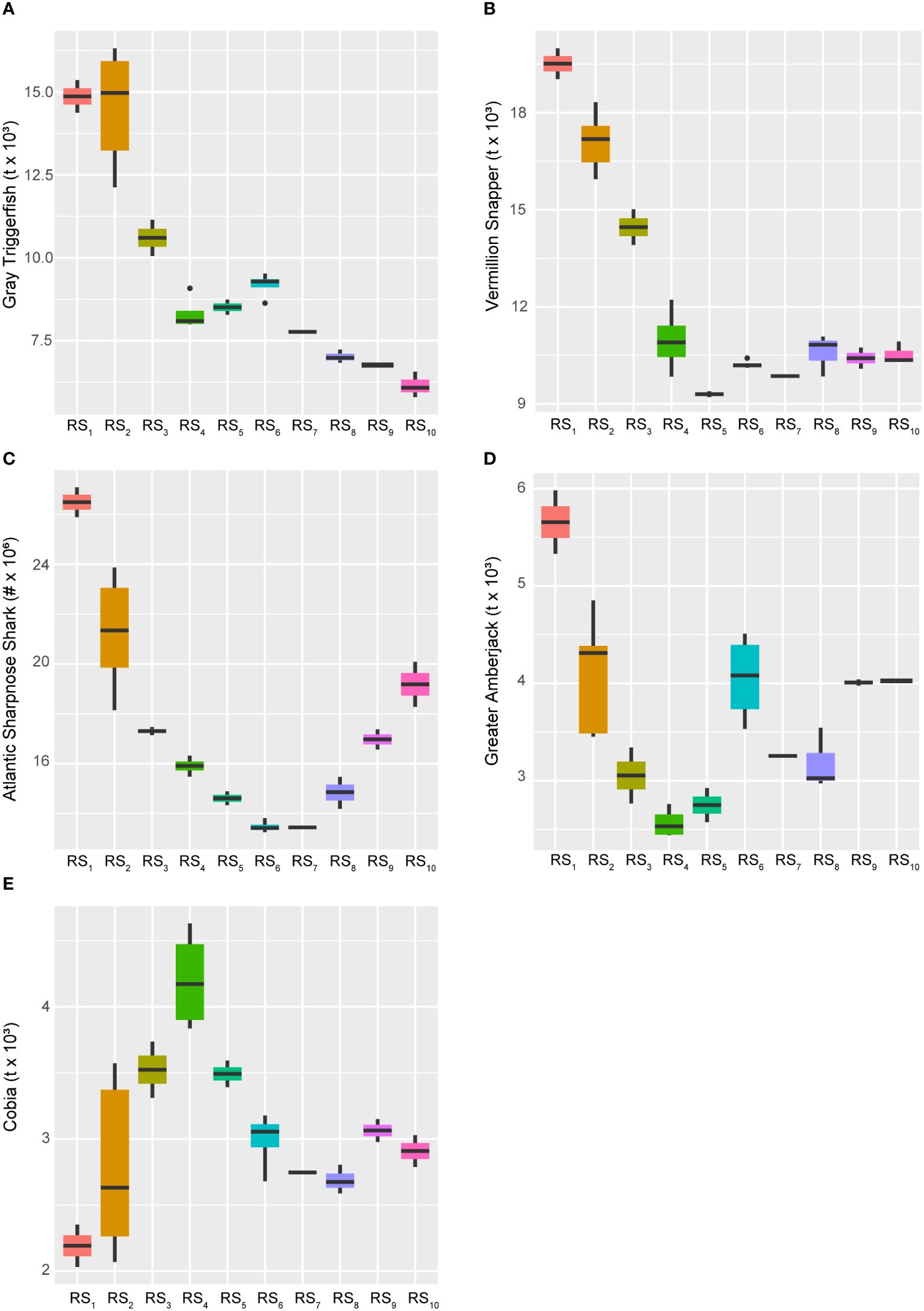
Figure 7 Boxplots across regimes for managed fishes displaying relative decreases over time. Panels depicting boxplots for the raw data distributions of upper-trophic-level fishery resource indicators in the GoM LME spanning 1986-2013. Fishery response indicators (Y) for Gray Triggerfish (A), Vermillion Snapper (B), Atlantic Sharpnose Shark (C), Greater Amberjack (D), and Cobia (E) displayed relative decreasing long-term trends over the study period. With the exception of Atlantic Sharpnose Sharks being reported as numbers of individuals, all species’ data represent biomass values. Colors correspond to the regime states (RSi) identified with DISPROF clustering of Y and match those used in previous figures and ordinations. Boxplots should be interpreted as follows: Horizontal lines depict the median value, and the lower and upper boundaries of each rectangle correspond to the 25th and 75th percentiles of the data, respectively. Whiskers extend to maxima and minima no more than 1.5x the inter-quartile range, and all other values are plotted as outliers (points). See Table 1 for indicator details and Table 5 for sample sizes.
4.2.2 Prey effects and the lower trophic levels
Close examination of the ordination diagram illustrating the GoM fishery ecosystem trajectory (Figure 4), confirms that the fishery resources were most responsive to the 28-year trend described above, and that species’ adjustments were differential throughout the trophic network. Within the LTL, the Gulf Menhaden index of abundance displayed a general increase over time, but with comparatively low values (Figure 8; Supplementary Figure S1) through RS2 (1988–1992), RS6-RS7 (2001–2005), and RS9 (2009–2010), potentially due to recruitment variability or other year-class effects (SEDAR, 2018). Alternatively, while the long-term trend indicates general growth of the menhaden population over time, it also implies a concurrent increase in the overall productivity of forage resources in the LME during the study period. Further, populations of Wood Storks and White Ibises were also highly responsive to this 28-year increasing trend, as were Roseate Spoonbills, albeit to a somewhat lesser degree (Figure 8). All three of these waterfowl species are indicative of the aquatic prey environment in the coastal habitats they reside within (Stolen et al., 2005; Karnauskas et al., 2013; Ogden et al., 2014). Therefore, their persistent increases over time, along with that of menhaden, likely signify that the coastal ecological system of the GoM is relatively healthy and not limiting the capacity of UTL fisheries or other living marine resources due to prey availability.
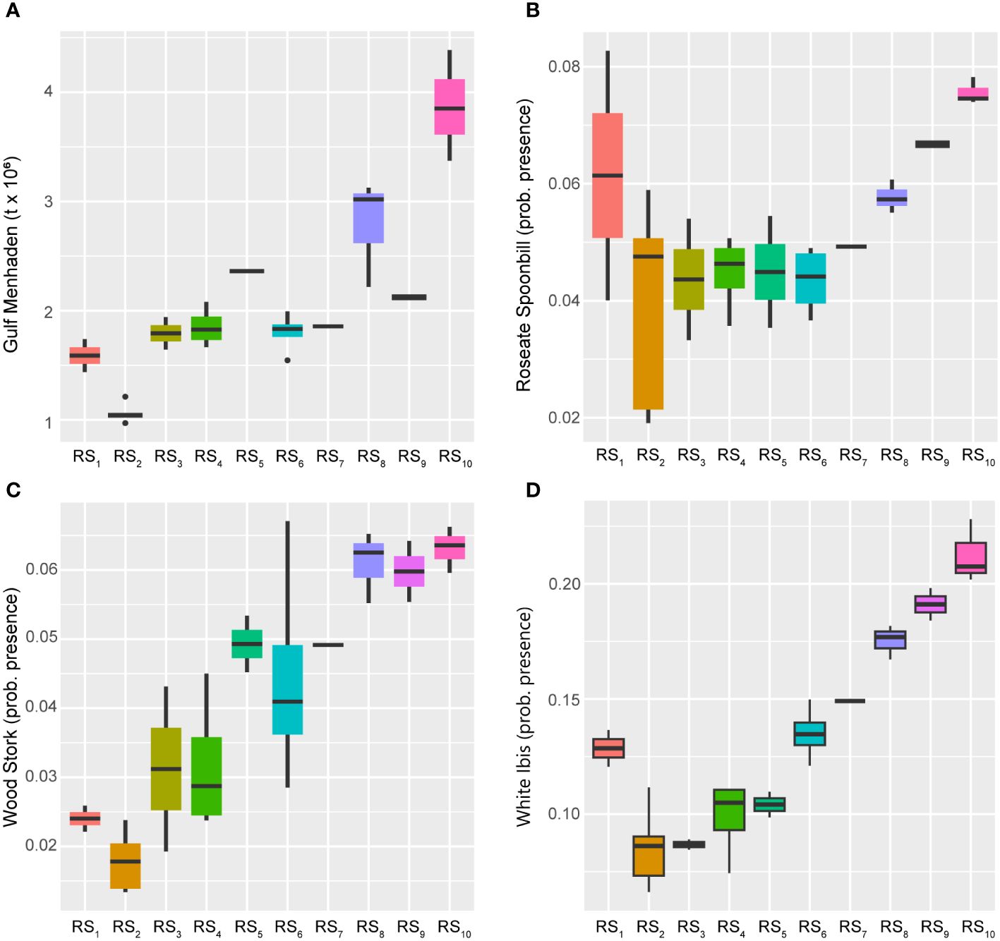
Figure 8 Boxplots across regimes for prey effects and lower-trophic-level indicators. Panels depicting boxplots for the raw data distributions of lower-trophic-level fishery resource indicators in the GoM LME spanning 1986-2013. Indicators were selected from the suite of fishery response data (Y) to characterize the status of the prey resources and the quality of coastal habitats. Gulf Menhaden (A) values represent biomass whereas the Roseate Spoonbill (B), Wood Stork (C), and White Ibis (D) indices all capture probability of presence. Colors correspond to the regime states (RSi) identified with DISPROF clustering of Y and match those used in previous figures and ordinations. Boxplots should be interpreted as follows: Horizontal lines depict the median value, and the lower and upper boundaries of each rectangle correspond to the 25th and 75th percentiles of the data, respectively. Whiskers extend to maxima and minima no more than 1.5x the inter-quartile range, and all other values are plotted as outliers (points). See Table 1 for indicator details and Table 5 for sample sizes.
4.2.3 Fishery capacity and ecosystem overfishing
The fishery capacity and ecosystem overfishing throughout the GoM LME have undergone significant changes over the study period, with complex associations with the dominant 28 and 14-year trends (Figure 4). What is apparent is the evidence pointing to a high-capacity but highly exploited fishery ecosystem during RS1-RS2 (1986–1992), with continued high exploitation and degradation during RS3-RS5 (1993–2000), and subsequent improvements throughout the remainder of the time series and the associated fishery regime states.
Relatively large populations of Magnificent Frigatebirds and Brown Pelicans indicate good health and high biocapacity of the marine ecosystem, as well as low pressures associated with fishing and pollution, respectively (Karnauskas et al., 2017a). Both indexes exhibited close inverse relationships with the 14-year trend (Figure 4), showing declining encounter rates through the first half of the time series (RS1-RS5) and increases after 2000 (Figure 9). These patterns align with the high exploitation rates that fisheries in the GoM LME experienced before the new management regulatory environment was introduced in the late-1990s (USDOC, 2007) and quota implementation moratoriums were lifted after 2000 (Hsu and Wilen, 1997). Additionally, given the current status as a highly regulated system, these gains appear to be persistent but continually evolving (Figure 5).
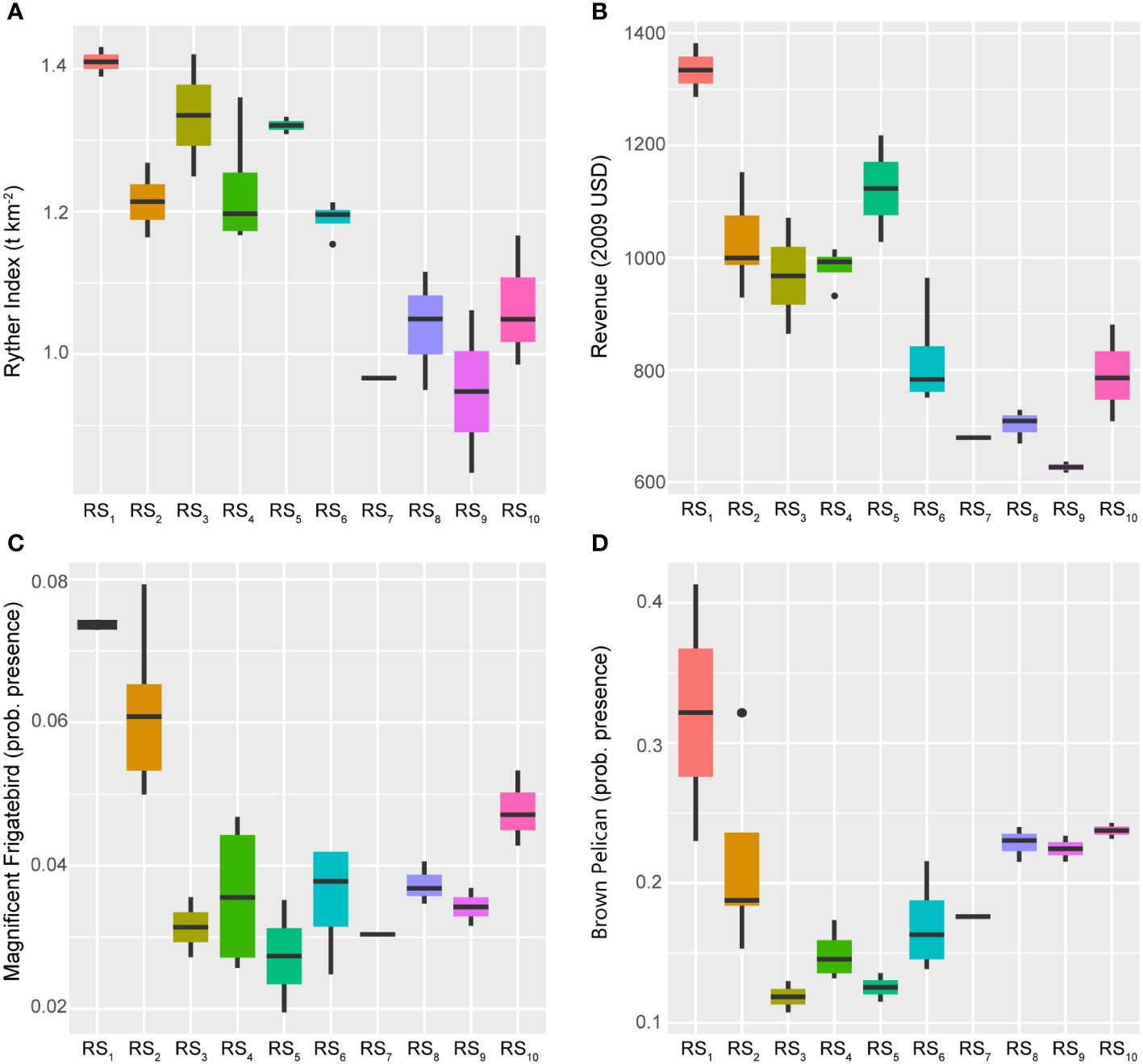
Figure 9 Boxplots across regimes for fishery capacity and ecosystem overfishing indicators. Panels depicting boxplots for the raw data distributions of various indicators capturing information about system-wide fishery removals and revenues (panels A, B) plus the health and biocapacity (panels C, D) of the GoM LME spanning 1986–2013. Indicators were selected from the suite of fishery response data (Y) where the Ryther index relates to a direct estimate of ecosystem overfishing for the LME, revenue values are adjusted to 2009 U.S. dollars (as of 2017 when the data were published), and waterfowl indices represent probabilities of presence. Colors correspond to the regime states (RSi) identified with DISPROF clustering of Y and match those used in previous figures and ordinations. Boxplots should be interpreted as follows: Horizontal lines depict the median value, and the lower and upper boundaries of each rectangle correspond to the 25th and 75th percentiles of the data, respectively. Whiskers extend to maxima and minima no more than 1.5x the inter-quartile range, and all other values are plotted as outliers (points). See Table 1 for indicator details and Table 5 for sample sizes.
The Ryther index of ecosystem overfishing more closely followed the longer 28-year trend (Figure 4) but was inversely related. The index substantially declined over the study period (Figure 9) from its historical high in RS1. Crucially, when interpreting the Ryther index, any values larger than 1.0 indicate an ecosystem that cannot sustain the level of removals being harvested from it (Link and Watson, 2019). Within this context, the GoM LME experienced unsustainable ecosystem overfishing throughout the 1980s and 1990s (RS1-RS5) that began to decline toward more sustainable levels after 2000 (Figure 9). However, it is notable that the Ryther index fell below the 1.0 threshold only four times over the 28 years studied in this analysis (2005, 2008, 2010, and 2013), all of which occurred after the paradigm shift in 1994/1995 (Figure 3; Supplementary Figure S1). This is likely a positive outcome (potentially due to management successes), but the uptick in this index over the final regime period (another response consistent with the Humpty Dumpty ecosystem trajectory) warrants further consideration. Regardless of the mechanisms that supported this contemporary increase, the end result is a move away from sustainable harvests at the scale of the fishery ecosystem.
4.2.4 Multispecies stock structure and function
From 1986 to 2013 the mean trophic level of FIM catches in the GoM described by the SEAMAP index showed a relative increase, primarily associated with the 28-year trend (albeit negatively); however, the 14-year cycle also appeared to influence these metrics to some degree. Overall, this loosely suggests that the trophic structure of the fisheries ecosystem may be stabilizing, leading to larger and more structured populations across various taxa within the LME’s food web (Pauly et al., 1998), or fishing “up” the food web (Shannon et al., 2014). When examined across the system’s regime states (Figure 10), there is a distinct peak in the index in RS7 (2005), followed by declines through subsequent years, but still ending at a relatively high point compared to the baseline period. This trajectory closely aligns with the Humpty Dumpty form displayed by the overall fishery ecosystem, further indicating that the fishery resources within the GoM LME represent a continuously changing dynamical system that switched modes of control in the mid-1990s.
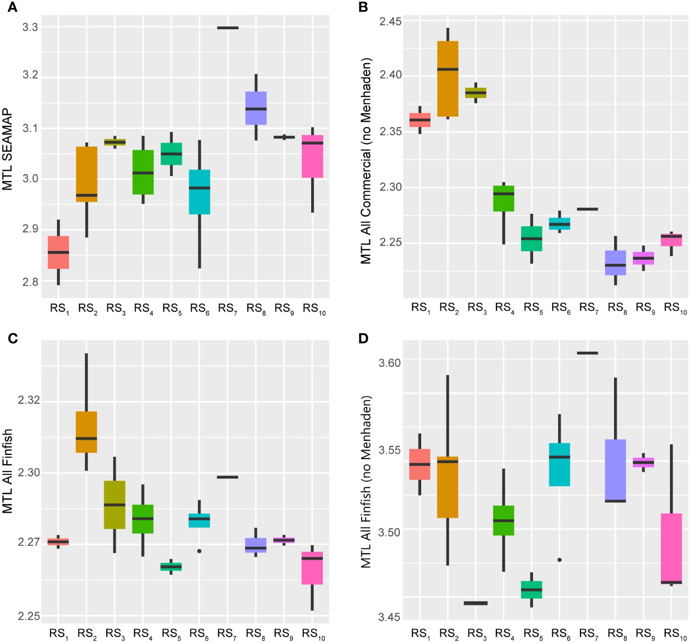
Figure 10 Boxplots across regimes for indicators of multispecies stock structure and function. Panels depicting boxplots for the raw data distributions of the mean trophic level (MTL) from fishery independent catches (A) and fishery dependent catches (panels B–D) in the GoM LME spanning 1986–2013. Indicators were selected from the suite of fishery response data (Y) to characterize the status, structure, and function of fishes and invertebrate catches in the region throughout the study period. Colors correspond to the regime states (RSi) identified with DISPROF clustering of Y and match those used in previous figures and ordinations. Boxplots should be interpreted as follows: Horizontal lines depict the median value, and the lower and upper boundaries of each rectangle correspond to the 25th and 75th percentiles of the data, respectively. Whiskers extend to maxima and minima no more than 1.5x the inter-quartile range, and all other values are plotted as outliers (points). See Table 1 for indicator details and Table 5 for sample sizes.
On the other hand, the MTLs of all commercial catches (vertebrates plus invertebrates, both with and without Gulf Menhaden) demonstrated evidence of decline over the study period, potentially indicating fishing “down” (Pauly et al., 1998; Karnauskas et al., 2017a) or “through” (Essington et al., 2006) the food web. While all derived from multispecies catches, this set of three indices is best interpreted as follows: one index that mainly captures trends in the MTL of Gulf Menhaden (‘MTL FinFish’), another more indicative of the trophic structure associated only with non-menhaden finfishes (‘MTL FinFish noMenh’), and a final index carrying information about trophic changes related to all combined catches by comprising lower-trophic-level invertebrates (i.e., shrimps) together with all non-menhaden finfishes (‘MTL AllComm noMenh’) (Karnauskas et al., 2017a). In all cases, the indices displayed relatively steep declines across the first five regimes (1986–2000), increases during the next two regimes (2001–2005), and then slightly divergent trends for the remaining years (Figure 10). The Gulf Menhaden MTL and the finfish-only MTL exhibited similarly domed trajectories across the final regime states (2006–2013), ultimately ending at near-time series lows. The combined invertebrate and finfish-only index showed slight increases over the remaining years but also ended at a relatively low value (Figure 10).
The observed trophic values spanned relatively small ranges, particularly for the Gulf Menhaden stock (0.09 TL units). Comparatively, the finfish and the combined invertebrate plus finfish indices displayed similar magnitudes of change (0.18 and 0.23 units, respectively). Interestingly, SEAMAP’s FIM index displayed the largest range of values, measuring 0.51 units. While the numerical magnitudes of these changes may not be alarming, it is concerning that the relative direction of all commercial fish catches’ MTLs was declining. The apparent stability of these catches may be misleading, as they are intrinsically commercially driven and fishers are incentivized to maintain marketable catches, which often translates to generally larger, upper-trophic-level fish being more desirable than smaller fish (Moeller and Engelken, 1972; Beardmore et al., 2015; Brinson and Wallmo, 2017). Thus, rather than relative trophic stability throughout the system over time, target species switching may be artificially maintaining these MTL values (Pauly et al., 1998; Essington et al., 2006; Shannon et al., 2014). Furthermore, their individual trends over time contribute to the contention that the controlling dynamics underlying the GoM LME, and its associated fishery resources, have shifted dramatically since the turn of the century, reflecting the Humpty Dumpty pattern once again (Figure 10).
4.3 Factors influencing the Gulf of Mexico fishery ecosystem’s organization over time
Over the 28-years examined in this study, the response of the GoM fishery ecosystem was modeled surprisingly well (R2adj = 0.7608) using only six synthetic temporal predictors (Figure 2; Table 3). Of those six AEMs, the first two (28 and 14-yr cycles) accounted for ~60% of that total explained variability (R2adj = 0.6029; Supplementary Table S1), were highly correlated with the first and second canonical axes of the final temporal RDA-model (Figure 4), respectively, and their axes weights (Supplementary Table S2) along those particular canonical dimensions far outweighed the remaining AEMs substantially contributing to the model. Thus, it is safe to conclude that there is a fair amount of continuous change (AEM-1) and, potentially, periodicity (AEM-2) inherent to the GoM LME and it’s living marine resources. The finer-scale AEMs (Figure 2) filled in the remaining details of the temporal model, but they provide no additional clarity and the final four canonical axes of the RDA model produced much more nuanced solutions than can be meaningfully interpreted (Supplementary Table S2).
To determine which specific mechanisms may be driving those patterns characterized in this study for the fishery ecosystem’s organization, the comprised ESR predictors were utilized in variable selection exercises against the final temporal model’s first two canonical axes. These efforts identified net-changes in petroleum industry related infrastructure (accounts for ~24% of total fishery ecosystem variability) and traditional artificial reef structures (~12%) as the top candidates for restructuring resources, followed by climate-related impacts (~6%), and recreational fishing effort (~1.5%). While these models capture the combined effects of all 23 response indicators among study years, it is still possible to tease out some of the internal dynamics associated with individual species as they relate to the holistic interpretation of the fishery ecosystem trajectory (Figure 4).
4.3.1 Artificial habitats
Considering the dominant 28-year trend captured by the first axis of the temporal model, it is sensible that factors such as the net-change in oil and gas industry platforms would be closely linked to this pattern. Over time, there has been a general decline in the annual installations of these platforms in the GoM LME (Figure 11) and starting in 1991 net-removals became commonplace (Supplementary Figure S2). Among the 28 years analyzed, the maximum net-change occurred in 1989 with the installation of 102 platforms. Notably, 15 of 28 years displayed net-removals, and from 2001–2013 (RS5-RS10) only 55 platforms were installed while another 1,437 were decommissioned throughout the region. On average, from 2001–2013, approximately 119 platforms were removed annually and in the last five years of the time series (RS9-RS10), this average jumps to -230 platforms each year.
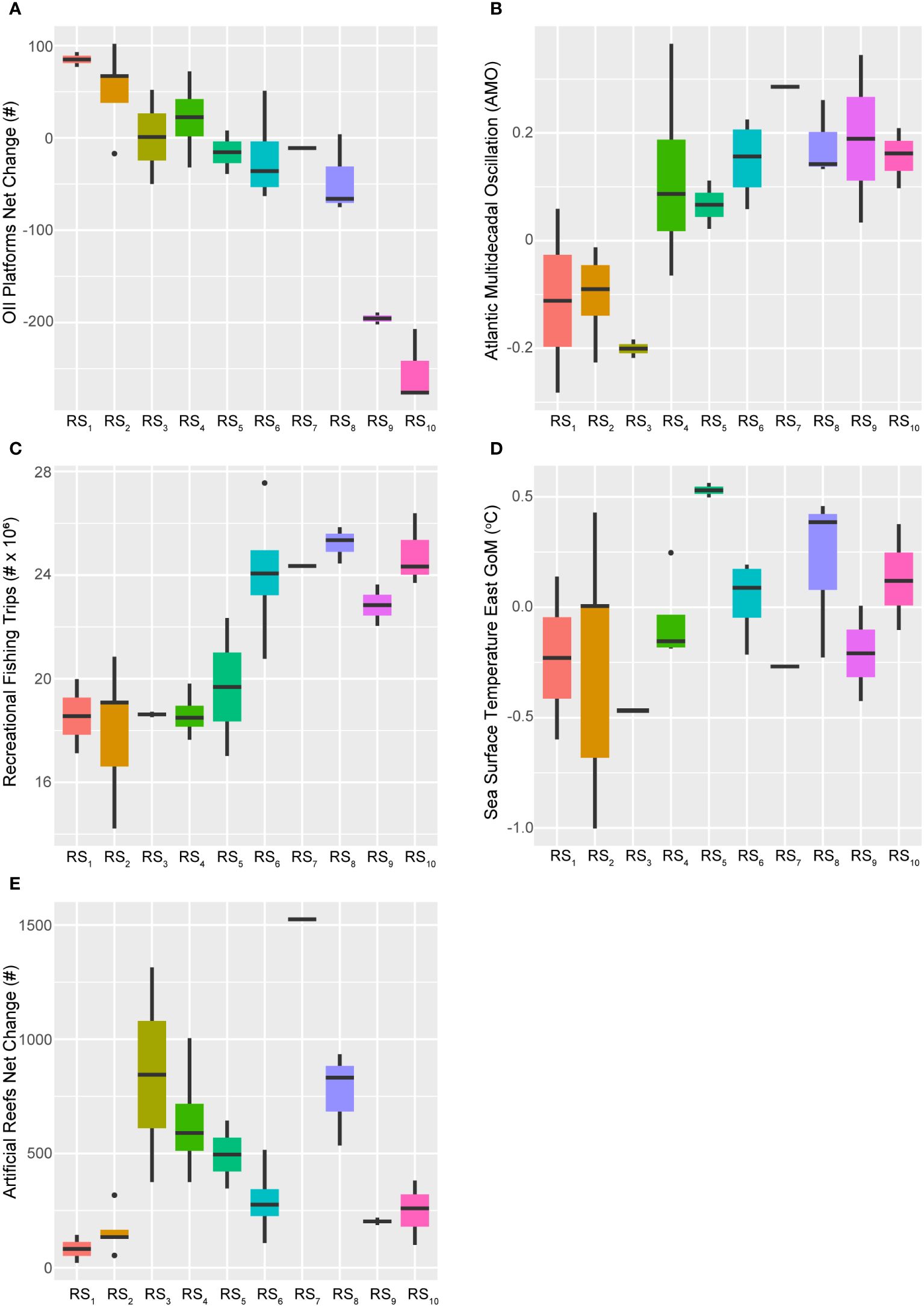
Figure 11 Boxplots across regimes for selected ecosystem status report predictors. Panels depicting boxplots for the raw data distributions of select ecosystem status report indicators (X*) spanning 1986-2013. This suite of descriptors best accounted for the first two canonical axes of the GoM fishery response's temporal model (RDAY|T*), and include the net-change in oil platforms (A), the Atlantic Multidecadal Oscillation index (B), recreational fishing trips taken (C), sea surface temperature in the eastern GoM (D), and the net-change in traditional artificial reef structures (E). Colors correspond to the regime states (RSi) identified with DISPROF clustering of the response data (Y) and match those used in previous figures and ordinations. Boxplots should be interpreted as follows: Horizontal lines depict the median value, and the lower and upper boundaries of each rectangle correspond to the 25th and 75th percentiles of the data, respectively. Whiskers extend to maxima and minima no more than 1.5x the inter-quartile range, and all other values are plotted as outliers (points). See Table 2 for indicator details and Table 5 for sample sizes.
The annual net-change in traditional artificial reef structures unrelated to the energy industry also exhibited a distinct temporal trend but it was modeled more closely by the 14-year cycle. Additionally, this predictor was also apparently influenced positively by AEM-5 and negatively by AEM-3 (Figure 4). More generally, the annual net-changes to this important fish habitat displayed a bimodal distribution throughout the study period, with peaks in 1994 (+1,314 reefs) and 2005 (+1,524 reefs). Although this index has never been negative (Supplementary Figure S2), periods of relatively low activity were observed through the first two (RS1-RS2) and the last two (RS9-RS10) fishery ecosystem regimes (Figure 11).
Artificial habitats are known to support a diversity of fishes in marine ecosystems, whether they are petroleum industry related (Seaman et al., 1989; Franks, 2000; Gallaway et al., 2021) or otherwise (Paxton et al., 2020a, b; Camp et al., 2022; Tharp et al., 2024). Industry related platforms are widely distributed throughout the northern and western GoM (Gardner et al., 2022), and 10 of the 11 federally managed fishes included in this analysis have been observed on these structures in recent investigations (Franks, 2000; Bolser et al., 2020; Gallaway et al., 2021), as have Gulf Menhaden (Gallaway et al., 2021). Furthermore, platforms have been estimated to support relatively substantial proportions of the Gulf-wide populations for Red and Vermillion Snappers (~5%) along with Cobia (~8%), and a shockingly high ~45% of the Greater Amberjack stock (Gallaway et al., 2021). Others have estimated ~7% of the Red Snapper population resides among the platform habitats of the region and further emphasizing their importance, particularly for juveniles and sub-adults (Karnauskas et al., 2017b). Thus, for some species (e.g., Greater Amberjack, Red Snapper) there is a line of evidence linking the decline in this critical habitat to the relative declines in their populations over time. However, disentangling this effect from other habitat relationships (i.e., traditional artificial reefs, natural systems) is not trivial, and would require focused effort. Furthermore, interpreting the presence of petroleum industry infrastructure as an indicator of oil and gas by-products entering the aquatic system and, subsequently, its associated living resources (Murawski et al., 2014; Pulster et al., 2020), could also help contextualize some of the differential responses (Murawski et al., 2021, 2023) observed here (Figure 4) and provide insights for future research.
Non-industry related, “traditional” artificial reef structures also play a critical role as fish habitat and, while the total number of petroleum platforms has declined, the total abundance of other structures (e.g., concrete rubble, vulcanized rubber, steel, and other metals/composites) has ballooned (Supplementary Figure S2). Over the study period, the net-change in industry related structures was -899 platforms, whereas other artificial reef installations included +12,355 new additions across the GoM. It should also be noted that, in addition to varying with respect to the materials used to build them, traditional artificial reef sizes can also be markedly different from one object to another (e.g., ranging from a chicken-coop to a sunken military vessel) and their spatial distributions throughout the GoM are highly irregular (Gardner et al., 2022). Along the U.S. east coast Gag, Greater Amberjack, and Red Snapper have all been observed taking full advantage of a wide selection of habitats available to them within acoustic telemetry arrays, including both artificial and natural reefs (Tharp et al., 2024). These authors, as well as others, implicate the possibility that for some fishes the critical aspect of most artificial reef structures is the vertical relief that they provide (Thompson et al., 2022; Tharp et al., 2024) and, therefore, their net-removal or -addition may be critically impacting fish distributions (Bolser et al., 2020; Paxton et al., 2020a). Greater Amberjack, in particular, may be susceptible to this effect given their proclivity for high-relief habitats (Gallaway et al., 2021; Bacheler et al., 2022; Tharp et al., 2024).
4.3.2 Climate and sea surface temperature
Variable selection of the 2017 ESR predictors lead to an optimal model that also included the AMO index and the time series of eastern GoM SST (SST East) values (Table 3). The AMO index accounted for ~6% of the total fishery ecosystem response while SST East captured < 1%, both indices displayed positive relationships with the 28-year trend in this system, and AMO was very strongly correlated with the major canonical axis in the final model (Figure 4). Consequently, these two indicators demonstrated general increases in their values over the study period, but they also displayed periods of relatively high and low activity (Figure 11). Both metrics capture changes in ecosystem and climate dynamics due to variability in water temperatures, with SST East serving as a more direct measurement for the GoM LME. The AMO index is based on SST dynamics in the north Atlantic Ocean (Schlesinger and Ramankutty, 1994) but it also carries information related to the teleconnected processes influenced by it (Enfield et al., 2001; Zhang et al., 2012; Nye et al., 2014), and which more directly affect the study region (Karnauskas et al., 2013; Kilborn et al., 2018). The inclusion of both a coarse- and fine-scale temperature-related variable in the final model suggests, as others have claimed (Geraldi et al., 2019), that this effect is not an artefact of measurement scale and that it is likely producing multifaceted effects across a number of potential mechanisms and scales (Levin, 1992).
The AMO index exhibits cyclical patterns on an approximately 65 to 70-year multidecadal scale (Schlesinger and Ramankutty, 1994) and around 1994/1995 it transitioned into a “warm phase” (Alexander et al., 2014) (Figure 11), signifying relatively greater mean surface water temperatures in the North Atlantic Ocean (Nye et al., 2014). Notable effects of the warm phase on the fishery ecosystem in the GoM LME include decreased concentrations of nitrate and dissolved oxygen in the Mississippi River outflow offshore Louisiana and Texas, along with increased terrestrial fertilizer inputs (potentially due to inland precipitation changes) and Gulf-wide maximum SST values (Kilborn et al., 2018). While the AMO index officially changed phases during the transition years from RS3 to RS4 (i.e., 1994/1995), over time there was an apparent ramp-up of the index as it approached its new, relatively higher mean value period (AMO1986–1994 = -0.13, AMO1995–1998 = 0.12, AMO1999–2013 = 0.16) with an absolute maximum in 1998 (AMO1998 = 0.37), and this transition lasted approximately four years.
The timing of this notable climate change index’s transition underscores the idea that a paradigm shift to a new set of underlying dynamics organizing the living marine resources in the GoM LME occurred after RS4. It also bolsters the idea that there is a lagged ecosystem-scale response that may take up to five years, as the temporal axes of control (Figure 3) for the GoM fishery ecosystem trajectory intersected in the AMO transition year and then diverged for roughly four to five years before running mostly parallel to each other for the remainder of the study period. The specific changes noted in the physio-chemical system, such as water temperatures, nitrate and oxygen concentrations, among others, were variable (Supplementary Figure S2). However, these new controlling dynamics likely altered the suite of species most likely to respond, positively or negatively, to the new conditions within the aquatic environment (Karnauskas et al., 2015; Kilborn et al., 2018).
As previously noted, the LTL resources modeled in this exercise were closely related to the primary axis of the RDA model (Figure 4), as were the majority of the federally managed UTL species included (Figure 4). Additionally, climatic variability has recently been shown to differentially affect many of this study’s UTL species across the long-term (Geraldi et al., 2019), while many short-lived forage species (e.g., Gulf Menhaden) and other LTL resources in the region have also been observed to differentially respond to climate-related variability, albeit on somewhat shorter timescales (Peake et al., 2022). In the GoM LME, Gulf Menhaden are an important prey species for key predators in this study, such as King and Spanish Mackerel, sharks, and other coastal piscivores (Berenshtein et al., 2023) like Red Grouper or Gag, while the population supports the largest commercial reduction fishery in the region (NMFS, 2023). Gulf Menhaden are typically more abundant during the cold/wet phase of the AMO (Sanchez-Rubio and Perry, 2015) and so the expectation would be that the population should have responded negatively to the AMO shift after RS4, but quite the opposite was observed here. These results may, in fact, be more related to socioeconomics than climatological factors, since at least one study indicated that the Gulf Menhaden stock was likely undergoing overfishing from the 1980s through the early 2000s (Berenshtein et al., 2023) and the sector’s fishing fleet was undergoing rapid transitions over the same period. The fleet’s size peaked at 82 vessels in 1982, was reduced to 58 by 1995, and continued dwindling down to 35 vessels by the final year of this study (SEDAR, 2018). These fleet adjustments effectively released considerable amounts of fishing pressure from this fishery over time and may have been influential to the population’s rebound. The reduction of menhaden fishing effort may also translate to gains in other fishes’ populations as well, given that some common predator species (e.g., sharks, Spanish Mackerel) are known to present at significant levels as fishery by-catch, and other UTL resources in the region were recently shown to respond more positively to reductions in menhaden effort than in effort directed at the target species (Berenshtein et al., 2021, 2023).
4.3.3 Recreational fishing
A single recreational fishing indicator was retained in the optimal model to account for the temporal variability along the 28-year axis: the total annual number of individual fishing trips taken. This index accounted for ~2% of the total fishery ecosystem variability, exhibited a consistent upward trend over time since its low point (14.2 million trips) in 1990 (Figure 11), and is strongly positively related to AEM-1 (Figure 4). During the initial period of controlling dynamics for the GoM fishery trajectory (RS1-RS4), this metric remained relatively low and stable, averaging around 18.4 million trips from 1986 to 1998. However, from 1999 onwards (RS5-RS10) there was a substantial 29% increase in the mean annual number of trips taken, reaching approximately 23.7 million trips from 1999 to 2013.
There appear to be both strong positive and negative correlations between the number of fishing trips taken and the relative biomass of many species, as well as potential impacts on ecosystem-wide multispecies metrics such as MTLs (Figure 4). While the underlying mechanisms behind these relationships are not fully understood, it is difficult to imagine an ecological scenario where substantially increased fishing pressure has resulted in long-term gains to populations. Indeed, studies have shown that it would be unwise to underestimate the impact of recreational fishing activities within the GoM LME (Coleman et al., 2004) and elsewhere (Geraldi et al., 2019). The significance of this fishery sector is further corroborated by the absence of commercial landings in the final optimal model, even though they were included in the pool of potential drivers considered to explain the fishery ecosystem’s response. Indeed, every UTL fish included in this study had a ratio of recreational to commercial catches > 1, and every species that was identified to be in long-term decline had a catch ratio > 2 (NMFS, 2023). Furthermore, those species which have been relatively resistant to management efforts (e.g., Cobia, Gray Triggerfish, Greater Amberjack) displayed very high recreational catches vs. their commercial counterparts, with Cobia displaying a system-wide high ratio of 33 (4.0 mp recreational catch vs. 0.12 mp commercial catch). Therefore, the reality of the likely impact of increased recreational fishing is that it has extended the exploitation period for some species and reduced their capacity to rebuild effectively (Neubauer et al., 2013), even in the face of stringent management efforts and reduced commercial extractions, particularly if enforcement is weak or broadly challenging (Melnychuk et al., 2017).
4.4 The Humpty Dumpty fish tale of the U.S. Gulf of Mexico
The Gulf of Mexico LME and its fishery resources have continuously reorganized over the nearly three decades analyzed in this study. These reorganizations were complex and multifaceted, often involving various species and ecosystem-level characteristics. The trajectory of this fishery ecosystem displayed gradual and persistent change over time, punctuated at its midpoint by a paradigm shift in the controlling dynamics organizing the living marine resources of the region that was most likely due to more effective management implementation resulting from the Sustainable Fisheries Act of 1996 coupled with a cool-to-warm phase-transition in the AMO around the same time. The GoM fishery ecosystem never maintained a relative stable state longer than five years. While it is possible that the system might be undergoing hysteresis on timescales beyond what was investigated here, it is more likely that, in addition to the natural variability related to environmental changes, the fishery ecosystem’s significant utilization rates and subsequent regulatory evolution led to gradual but irreversible changes, akin to the popular children’s nursery rhyme of Humpty Dumpty.
Humpty Dumpty sat on a wall.
Humpty Dumpty had a great fall.
All the King’s horses, and all the King’s men,
Couldn’t put Humpty together again.
Among those organizing factors investigated, changes to artificial reef prevalence and recreational fishing pressure were shown to impact resource shifts at magnitudes and scales similar to those from climate change related phenomena. Additionally, considering the history of high exploitation and the timing of effective management implementation, it is reasonable to conclude that fishery management in the GoM region played a substantial role in the paradigm shift after the mid-1990s, alongside that of the AMO transition and all that it encapsulates.
Unfortunately, the interplay between intensive and fluctuating fishing pressure, natural and anthropogenic drivers, and management or socioeconomic responses resulted in low-grade degradation of the trophic structure of living marine resources over time and a contemporary fishery ecosystem that remained relatively overfished as of 2013. Although there was significant improvement in this adjudication over the study period, most likely due to management intervention and success, the precise mechanisms and contributing factors remain poorly understood. Furthermore, while changes in fishing regulations do offer sustainable options for administering living marine resources, the speed and uncertainty associated with climate-related changes compared to the speed of management presents some challenges. Furthermore, the fishery ecosystem and the resources that it comprises may respond differentially to any one management action, making the whole endeavor, perhaps, even more challenging.
However, when viewed comprehensively – and unlike the Humpty Dumpty from the children’s tale – the Gulf of Mexico fishery ecosystem has demonstrated considerable resilience and improvement of its status over time, potentially due to its complexity and diversity. However, it is not immune to changing socioeconomic and environmental conditions, nor can it be said to be overly predictable or stable. Fishing activity and management decisions apparently exert substantial control over the underlying fishery resource dynamics, although the local influence of warming waters and the effects of drastically evolving global climate conditions may interact with these controls in unpredictable ways. The Humpty Dumpty ecosystem trajectory suggests that the GoM LME’s resources will continue to reorganize on relatively short timescales and may display undesirable (or desirable) emergent behaviors in the future. Consequently, the system will likely not be managed toward any one historically pristine or desirable long-term stable state, at least not for very long. This makes prioritizing effective EBFM solutions for the region all the more important, as they contain recursive and regular updates of system-wide status and contemporary risk assessments. As the evidence shows, the moral of the Humpty Dumpty fish tale for the Gulf of Mexico is that differential species’ responses and continuous reorganizations of living marine resources are the norm for this LME. Therefore, it is likely best to manage these critical public trust resources cautiously in the face of uncertainty.
4.5 Limitations, uncertainties, and future work
The AEM framework and modeling methods employed here were used to develop purely synthetic temporal predictors for explicitly modeling multi-scale patterns in the set of multivariate responses comprised to describe the GoM fishery ecosystem. These patterns were further investigated to determine if any particular ecological covariates were similarly structured over time, and which (if any) inferences might be made about the timing of independently derived regime state changes and any connectivity among the descriptors included in the models.
After developing the purely temporal, AEM model of the GoM LME that accounted for ~76% of the total fishery ecosystem response over 28 years, the AIC variable selection process identified five additional ecosystem-level factors that covaried temporally, and no additional ESR indicators were selected to account for the residual variability from the RDAY|T* model (i.e., non-temporally structured fishery ecosystem response). The variation partitioning results (Table 4) revealed that, of the total fishery ecosystem variability explained by the six synthetic AEMs, approximately 48% of that – or approximately 36% of the total variability – was attributable to the selected, temporally structured, ecosystem covariates. The implication being that the remaining ~40% of the total fishery ecosystem response that was accounted for by the AEM model could not be attributed to any other ESR variable included in the selection process (Table 2). This presents the scenario where some temporally structured characteristics of the GoM LME remain unaccounted for while still apparently contributing substantially to the long-term organization of living marine resources in the region.
Recall, the representation of the fishery ecosystem and the optimal model to describe it were intentionally limited to those indicators drawn from the 2017 ESR and the Ryther index (Table 2). The purpose for doing so was to present a case-study for the distillation of the milieu of information contained within an ESR using a method that could track historical changes in the system’s state and potentially identify leading indicators (or drivers) of system-wide shifts. The practical result of such a decision, however, is a relatively naïve compilation of descriptors to draw from that may not represent all of the “most important” aspects of the fishery ecosystem or the LME. This is also complicated by parameters’ inclusion in or removal from subsequent reports (Karnauskas et al., 2013; Karnauskas et al., 2017a), and the application of these methods may be more effective in regions where the list of ESR indicators are relatively stable and/or regularly updated. Indeed, previous work indicated that some predictors from the 2013 ESR were important to the fishery ecosystem outcomes, such as menhaden fishing effort, fertilizer usage in the MARB watershed, zooplankton abundance, and ichthyoplankton abundance (Karnauskas et al., 2015; Kilborn et al., 2018), but they were not included in the 2017 update and could not be added to this effort. Other notable descriptors were not available for this study due to missing data at the start of the time series (e.g., dissolved oxygen), or they were simply excluded from in the 2017 ESR (e.g., shrimp indices of abundance).
Further, when considering indices of ecosystem overfishing, the use of more than one metric is recommended (Link and Watson, 2019) and only the Ryther index was utilized here. This represents an instance where the original intention to exclusively use ESR data was suspended, however, the inclusion of more than one index was disallowed due to mismatches in the time series that were obtained from Link and Watson (2019). Of the three time series received – one each for the Ryther, Fogarty, and Friedland indices – only the Ryther index covered the period of this analysis, whereas the other two were only calculated from 1997 onward. Further, both of the shorter metrics were highly correlated (r < 0.85) with the Ryther index across their paired series’, and the Fogarty and Friedland ratios displayed even higher levels of correspondence (r = 0.94). Thus, in keeping with the spirit of using easily obtainable data drawn from as few sources as possible (i.e., the ESRs), the decision to only include the Ryther index was made.
It should also be noted that, while many of the implications of this study relate to the impacts of fisheries management, no explicit descriptors that carried information about management decision making or rule enforcement were included in these analyses. Therefore, future work might incorporate specific measures of when critical management actions were implemented so that their effects might be scrutinized more closely. This would not be a trivial exercise, however, since many species have undergone dozens of regulatory changes since the mid-1990s, see Red Snapper (SEDAR, 2024) and Greater Amberjack as recent examples (SEDAR, 2020).
In addition to the challenges associated with indicator selection, the relatively straightforward approach to model building used here seeks to identify non-random numerical relationships between predictors and responses within the pool of descriptors assembled to conceptualize these LME sub-systems. Therefore, while the system-wide responses and selected predictors may offer insights into potential broad-scale dynamics within the LME, further exploration is warranted to adequately assign mechanistic status to these relations with a high degree of certainty.
Lastly, the uncharacterized purely temporal fraction of explained variability (~28%) from the final model and the substantial amount of remaining unexplained variability (~24%) both represent significant proportions of the GoM fishery ecosystem that deserve greater attention. The forces and dynamics controlling these aspects likely also play a crucial role in determining the holistic organization of living marine resources in the LME. Identifying and incorporating these missing elements into future research and modeling efforts is essential for a more comprehensive understanding of GoM fishery ecosystem’s dynamics, particularly within an EBFM framework. Doing so will provide scientists and policymakers with deeper insights into the complex interactions governing the GoM LME, thus enabling more informed and effective management strategies for the sustainable conservation of marine resources moving forward.
Data availability statement
Publicly available datasets were analyzed in this study. This data can be found here: https://www.aoml.noaa.gov/ocd/ocdweb/ESR_GOMIEA/download.html.
Author contributions
JPK: Conceptualization, Data curation, Formal analysis, Funding acquisition, Investigation, Methodology, Project administration, Resources, Software, Supervision, Validation, Visualization, Writing – original draft, Writing – review & editing.
Funding
The author(s) declare financial support was received for the research, authorship, and/or publication of this article. Funding for this work was provided by the NOAA National Marine Fisheries Service grant NA17NMF4330318.
Acknowledgments
The author would like to thank Dr. Michael Drexler from the Ocean Conservancy and Dr. Mandy Karnauskas from the National Oceanic and Atmospheric Administration for feedback on early iterations of this work. Additional thanks go to the Gulf of Mexico Fishery Management Council Science and Statistical Committee members for their clarifying questions and commentary. Finally, thank you to the peer-reviewers that helped improve the quality of this manuscript based upon their insightful consideration of this work.
Conflict of interest
The author declares that the research was conducted in the absence of any commercial or financial relationships that could be construed as a potential conflict of interest.
Publisher’s note
All claims expressed in this article are solely those of the authors and do not necessarily represent those of their affiliated organizations, or those of the publisher, the editors and the reviewers. Any product that may be evaluated in this article, or claim that may be made by its manufacturer, is not guaranteed or endorsed by the publisher.
Supplementary material
The Supplementary Material for this article can be found online at: https://www.frontiersin.org/articles/10.3389/fmars.2024.1333756/full#supplementary-material
References
Akaike H. (1974). A new look at the statistical model identification. IEEE Trans. Autom. Control, AC1 9 (6), 716–723. AC19. doi: 10.1109/TAC.1974.1100705
Alexander M. A., Halimeda Kilbourne K., Nye J. A. (2014). Climate variability during warm and cold phases of the Atlantic Multidecadal Oscillation (AMO) 1871–2008. J. Mar. Syst. 133, 14–26. doi: 10.1016/j.jmarsys.2013.07.017
Anderson M. J., Willis T. J. (2003). Canonical analysis of principal coordinates: A useful method of constrained ordination for ecology. Ecology 84, 511–525. doi: 10.1890/0012-9658(2003)084[0511:CAOPCA]2.0.CO;2
Andrews K. S., Williams G. D., Gertseva V. V. (2014). California Current Integrated Ecosystem Assessment, Phase III Report: Anthropogenic Drivers and Pressures. Eds. Harvey C. J., Garfield E. L., Hazen E. L., Williams G. D. (Seattle, WA: NOAA, Northwest Fisheries Science Center).
Angeler D. G., Allen C. R., Johnson R. K. (2013). Measuring the relative resilience of subarctic lakes to global change: redundancies of functions within and across temporal scales. J. Appl. Ecol. 50, 572–584. doi: 10.1111/1365-2664.12092
Bacheler N. M., Gregalis K. C., Gillum Z. D., Pickett E. P., Schobernd C. M., Schobernd Z. H., et al. (2022). Using stationary video data to infer relative abundance and distribution of four Seriola species along the southeast United States Atlantic coast. Fish. Res. 249, 106238. doi: 10.1016/j.fishres.2022.106238
Baho D. L., Futter M. N., Johnson R. K., Angeler D. G. (2015). Assessing temporal scales and patterns in time series: Comparing methods based on redundancy analysis. Ecol. Complex. 22, 162–168. doi: 10.1016/j.ecocom.2015.04.001
Beardmore B., Hunt L. M., Haider W., Dorow M., Arlinghaus R. (2015). Effectively managing angler satisfaction in recreational fisheries requires understanding the fish species and the anglers. Can. J. Fish. Aquat. Sci. 72, 500–513. doi: 10.1139/cjfas-2014-0177
Beisner B. E., Haydon D. T., Cuddington K. (2003). Alternative stable states in ecology. Front. Ecol. Environ. 1, 376–382. doi: 10.1890/1540-9295(2003)001[0376:ASSIE]2.0.CO;2
Berenshtein I., Sagarese S. R., Lauretta M. V., Nuttall M. A., Chagaris D. D. (2021). Technical documentation of a U.S. Gulf of Mexico-wide Ecosystem model (Washington, DC: NOAA, U.S. Department of Commerce).
Berenshtein I., Sagarese S. R., Lauretta M. V., Schueller A. M., Chagaris D. D. (2023). Identifying trade-offs and reference points in support of ecosystem approaches to managing Gulf of Mexico menhaden. Front. Mar. Sci. 9. doi: 10.3389/fmars.2022.935324
Blanchet F. G., Legendre P., Borcard D. (2008a). Forward selection of explanatory variables. Ecology 89, 2623–2632. doi: 10.1890/07-0986.1
Blanchet F. G., Legendre P., Borcard D. (2008b). Modelling directional spatial processes in ecological data. Ecol. Model. 215, 325–336. doi: 10.1016/j.ecolmodel.2008.04.001
Blanchet F. G., Legendre P., Maranger R., Monti D., Pepin P. (2011). Modelling the effect of directional spatial ecological processes at different scales. Oecologia 166, 357–368. doi: 10.1007/s00442-010-1867-y
Boldt J. L., Thompson M., Rooper C. N., Hay D. E., Schweigert J. F., Quinn T. J., et al. (2019). Bottom-up and top-down control of small pelagic forage fish: factors affecting age-0 herring in the Strait of Georgia, British Columbia. Mar. Ecol. Prog. Ser. 617–618, 53–66. doi: 10.3354/meps12485
Bolser D. G., Egerton J. P., Grüss A., Loughran T., Beyea T., Mccain K., et al. (2020). Environmental and Structural Drivers of Fish Distributions among Petroleum Platforms across the US Gulf of Mexico. Mar. Coast. Fish. 12, 142–163. doi: 10.1002/mcf2.10116
Borcard D., Legendre P., Drapeau P. (1992). Partialling out the spatial component of ecological variation. Ecology 73, 1045–1055. doi: 10.2307/1940179
Branch T. A., Watson R., Fulton E. A., Jennings S., Mcgilliard C. R., Pablico G. T., et al. (2010). The trophic fingerprint of marine fisheries. Nature 468, 431–435. doi: 10.1038/nature09528
Brinson A. A., Wallmo K. (2017). Determinants of saltwater anglers’ Satisfaction with fisheries management: regional perspectives in the United States. North Am. J. Fish. Manage. 37, 225–234. doi: 10.1080/02755947.2016.1235629
Camp E. V., Chong L., Collins A. B., Abeels H., Mille K., Hall-Scharf B., et al. (2022). An update on Florida’s artificial reefs: recent research and what it means for Florida: FA245, 10/2022. EDIS 5, 1–8. doi: 10.32473/edis-fa245-2022
Clarke K. R., Somerfield P. J., Chapman M. G. (2006). On resemblance measures for ecological studies, including taxonomic dissimilarities and a zero-adjusted Bray-Curtis coefficient for denuded assemblages. J. Exp. Mar. Biol. Ecol. 330, 55–80. doi: 10.1016/j.jembe.2005.12.017
Clarke K. R., Somerfield P. J., Gorley R. N. (2008). Testing of null hypotheses in exploratory community analyses: similarity profiles and biota-environment linkage. J. Exp. Mar. Biol. Ecol. 366, 56–69. doi: 10.1016/j.jembe.2008.07.009
Coleman F. C., Figueira W. F., Ueland J. S., Crowder L. B. (2004). The impact of United States recreational fisheries on marine fish populations. Science 305, 1958–1960. doi: 10.1126/science.1100397
Cordes E. E., Jones D. O. B., Schlacher T. A., Amon D. J., Bernardino A. F., Brooke S., et al. (2016). Environmental impacts of the deep-water oil and gas industry: A review to guide management strategies. Front. Environ. Sci. 4, 26. doi: 10.3389/fenvs.2016.00058
Dell’Apa A., Kilborn J. P., Harford W. J. (2020). Advancing ecosystem management strategies for the Gulf of Mexico's fisheries resources: implications for the development of a fishery ecosystem plan. Bull. Mar. Sci. 96, 000–000. doi: 10.5343/bms.2019.0081
D’Errico J. (2009) SLM-Shape Language Modeling. Available at: https://www.mathworks.com/matlabcentral/fileexchange/24443-slm-shape-language-modeling:Mathworks.
Deyoung B., Barange M., Beaugrand G., Harris R., Perry R. I., Scheffer M., et al. (2008). Regime shifts in marine ecosystems: detection, prediction and management. Trends Ecol. Evol. 23, 402–409. doi: 10.1016/j.tree.2008.03.008
Diekmann R., Mollmann C. (2010). Integrated ecosystem assessments of seven Baltic Sea areas covering the last three decades. ICES Coop. Res. Rep. 302, 1–90. doi: 10.17895/ices.pub.5413
Enfield D. B., Mestas-Nunez A. M., Trimble P. J. (2001). The Atlantic multidecadal oscillation and its relation to rainfall and river flows in the continental US. Geophys. Res. Lett. 28, 2077–2080. doi: 10.1029/2000GL012745
Essington T. E., Beaudreau A. H., Wiedenmann J. (2006). Fishing through marine food webs. Proc. Natl. Acad. Sci. United States America 103, 3171–3175. doi: 10.1073/pnas.0510964103
Faith D. P., Minchin P. R., Belbin L. (1987). Compositional dissimilarity as a robust measure of ecological distance. Vegetatio 69, 57–68. doi: 10.1007/BF00038687
Franks J. (2000). A review: pelagic fishes at petroleum platforms in the Northern Gulf of Mexico; diversity, interrelationships, and perspective. Pêche thonière et dispositifs de concentration de poissons, Caribbean-Martinique, 15-19 Oct 1999. Available at: https://archimer.ifremer.fr/doc/00042/15301/.
Gallaway B. J., Raborn S. W., Mccain K. A., Beyea R. T., Dufault S., Heyman W., et al. (2021). Absolute abundance estimates for red snapper, greater amberjack, and other federally managed fish on offshore petroleum platforms in the gulf of Mexico. North Am. J. Fish. Manage. 41, 1665–1690. doi: 10.1002/nafm.10678
Gardner C., Goethel D. R., Karnauskas M., Smith M. W., Perruso L., Walter J. F. (2022). Artificial attraction: linking vessel monitoring system and habitat data to assess commercial exploitation on artificial structures in the gulf of Mexico. Front. Mar. Sci. 9. doi: 10.3389/fmars.2022.772292
Geraldi N. R., Kellison G. T., Bacheler N. M. (2019). Climate indices, water temperature, and fishing predict broad scale variation in fishes on temperate reefs. Front. Mar. Sci. 6, 13. doi: 10.3389/fmars.2019.00030
Gotelli N. J., Ellison A. M. (2004). A primer of ecological statistics. Sunderland, MA: Sinauer Associates Publishers.
Grimes C. B., Finucane J. H. (1991). Spatial-distribution and abundance of larval and juvenile fish, chlorophyll and macrozooplankton around the Mississippi River discharge plume, and the role of the plume in fish recruitment. Mar. Ecol. Prog. Ser. 75, 109–119. doi: 10.3354/meps075109
Helfman G. S., Collette B. B., Facey D. E., Bowen B. W. (2009). The diversity of fishes: biology, evolution, and ecology (Chichester, UK; Hoboken, NJ: Blackwell).
Holland S. M., Ditton R. B. (1992). Fishing trip satisfaction: A typology of anglers. North Am. J. Fish. Manage. 12, 28–33. doi: 10.1577/1548-8675(1992)012<0028:FTSATO>2.3.CO;2
Hsu S. L., Wilen J. E. (1997). Ecosystem management and the 1996 sustainable fisheries act. Ecol. Law Q. 24, 799–811. Available at: https://www.jstor.org/stable/24113293
Jones D. L. (2017). The Fathom Toolbox for MATLAB: Software for multivariate ecological and oceanographic analysis (St. Petersburg, FL, USA: University of South Florida, College of Marine Science). Available at: https://www.marine.usf.edu/research/matlab-resources/.
Karnauskas M., Kelble C. R., Regan S., Quenée C., Allee R., Jepson M., et al. (2017a). 2017 Ecosystem status report update for the Gulf of Mexico (Miami, FL: NOAA, Southeast Fisheries Science Center).
Karnauskas M., Schirripa M. J., Craig J. K., Cook G. S., Kelble C. R., Agar J. J., et al. (2015). Evidence of climate-driven ecosystem reorganization in the Gulf of Mexico. Global Change Biol. 21, 2554–2568. doi: 10.1111/gcb.12894
Karnauskas M., Schirripa M. J., Kelble C. R., Cook G. S., Craig J. K., N. U.S. Department of Commerce (2013). Ecosystem status report for the Gulf of Mexico (Miami, FL: NOAA, Southeast Fisheries Science Center).
Karnauskas M., Walter Iii J. F., Campbell M. D., Pollack A. G., Drymon J. M., Powers S. (2017b). Red snapper distribution on natural habitats and artificial structures in the northern gulf of Mexico. Mar. Coast. Fish. 9, 50–67. doi: 10.1080/19425120.2016.1255684
Kelble C. R., Loomis D. K., Lovelace S., Nuttle W. K., Ortner P. B., Fletcher P., et al. (2013). The EBM-DPSER conceptual model: integrating ecosystem services into the DPSIR framework. PloS One 8, e70766. doi: 10.1371/journal.pone.0070766
Kilborn J. P. (2020). The Darkside Toolbox for MATLAB (St. Petersburg, FL: University of South Florida, College of Marine Science).
Kilborn J. P., Drexler M., Jones D. L. (2018). Fluctuating fishing intensities and climate dynamics reorganize the Gulf of Mexico’s fisheries resources. Ecosphere 9, e02487. doi: 10.1002/ecs2.2487
Kilborn J. P., Jones D. L., Peebles E. B., Naar D. F. (2017). Resemblance profiles as clustering decision criteria: Estimating statistical power, error, and correspondence for a hypothesis test for multivariate structure. Ecol. Evol. 7, 2039–2057. doi: 10.1002/ece3.2760
Kildow J., Colgan C., Johnston P., Scorse J., Farnum M. (2016). State of the U.S. Ocean and coastal economies: 2016 update. Public. Natl. Ocean Econ. Program 35, 1–35. Available at: https://cbe.miis.edu/noep_publications/18.
Kildow J. T., Colgan C. S., Scorse J. D., Johnston P., Nichols M. (2014). State of the U.S. Ocean and coastal economies 2014. Public. Natl. Ocean Econ. Program 82, 1–82. Available at: https://cbe.miis.edu/noep_publications/1.
Kumpf H., Steidinger K. A., Sherman K. (1999). The Gulf of Mexico large marine ecosystem: assessment, sustainability, and management (Malden, Mass., USA: Blackwell Science).
Lamothe K. A., Jackson D. A., Somers K. M. (2017). Utilizing gradient simulations for quantifying community-level resistance and resilience. Ecosphere 8, e01953. doi: 10.1002/ecs2.1953
Lamothe K. A., Somers K. M., Jackson D. A. (2019). Linking the ball-and-cup analogy and ordination trajectories to describe ecosystem stability, resistance, and resilience. Ecosphere 10, 11. doi: 10.1002/ecs2.2629
Legendre P., Anderson M. J. (1999). Distance-based redundancy analysis: Testing multispecies responses in multifactorial ecological experiments. Ecol. Monogr. 69, 1–24. doi: 10.1890/0012-9615(1999)069[0001:DBRATM]2.0.CO;2
Legendre P., Gauthier O. (2014). Statistical methods for temporal and space-time analysis of community composition data. Proc. R. Soc. B-Biol. Sci. 281, 9. doi: 10.1098/rspb.2013.2728
Levin S. A. (1992). The problem of pattern and scale in ecology. Ecology 73, 1943–1967. doi: 10.2307/1941447
Levin P. S., Fogarty M. J., Murawski S. A., Fluharty D. (2009). Integrated ecosystem assessments: developing the scientific basis for ecosystem-based management of the ocean. PloS Biol. 7, e1000014. doi: 10.1371/journal.pbio.1000014
Link J. (2016a). Ecosystem-Based Fisheries Management Policy. National Marine Fisheries Service, Washington, DC: U.S. Department of Commerce, NOAA. Report No.: NMFSPD 01-120.
Link J. (2016b). NOAA Fisheries Ecosystem-Based Fisheries Management Road Map (Washington, DC: U.S. Department of Commerce, NOAA). National Marine Fisheries Service.
Link J. S., Brodziak J. K. T., Edwards S. F., Overholtz W. J., Mountain D., Jossi J. W., et al. (2002). Marine ecosystem assessment in a fisheries management context. Can. J. fish. Aquat. Sci. 59, 1429–1440. doi: 10.1139/f02-115
Link J. S., Watson R. A. (2019). Global ecosystem overfishing: Clear delineation within real limits to production. Sci. Adv. 5, eaav0474. doi: 10.1126/sciadv.aav0474
MacIntosh A., Dafforn K., Penrose B., Chariton A., Cresswell T. (2022). Ecotoxicological effects of decommissioning offshore petroleum infrastructure: A systematic review. Crit. Rev. Environ. Sci. Technol. 52, 3283–3321. doi: 10.1080/10643389.2021.1917949
Melnychuk M. C., Peterson E., Elliott M., Hilborn R. (2017). Fisheries management impacts on target species status. Proc. Natl. Acad. Sci. United States America 114, 178–183. doi: 10.1073/pnas.1609915114
Miller J. K. (1975). The sampling distribution and a test for the significance of the bimultivariate redundancy statistic: a Monte Carlo study. Multivariate Behav. Res. 10, 233–244. doi: 10.1207/s15327906mbr1002_8
Moeller G. H., Engelken J. H. (1972). What fishermen look for in a fishing experience. J. Wildl. Manage. 36, 1253–1257. doi: 10.2307/3799256
Mollmann C., Diekmann R. (2012). “Marine ecosystem regime shifts induced by climate and overfishing: a review for the northern hemisphere,” in Advances in Ecological Research, Vol 47: Global Change in Multispecies Systems, Pt 2. Eds. Woodward G., Jacob U., Ogorman E. J. (Elsevier Academic Press Inc, San Diego), 303–347.
Murawski S. A., Hogarth W. T., Peebles E. B., Barbeiri L. (2014). Prevalence of external skin lesions and polycyclic aromatic hydrocarbon concentrations in gulf of Mexico fishes, post-deepwater horizon. Trans. Am. Fish. Soc. 143, 1084–1097. doi: 10.1080/00028487.2014.911205
Murawski S. A., Kilborn J. P., Bejarano A. C., Chagaris D., Donaldson D., Hernandez F. J., et al. (2021). A synthesis of deepwater horizon impacts on coastal and nearshore living marine resources. Front. Mar. Sci. 7. doi: 10.3389/fmars.2020.594862
Murawski S. A., Schwing P. T., Patterson W. F., Sutton T. T., Montagna P. A., Milligan R. J., et al. (2023). Vulnerability and resilience of living marine resources to the Deepwater Horizon oil spill: an overview. Front. Mar. Sci. 10. doi: 10.3389/fmars.2023.1202250
Neubauer P., Jensen O. P., Hutchings J. A., Baum J. K. (2013). Resilience and recovery of overexploited marine populations. Science 340, 347–349. doi: 10.1126/science.1230441
NMFS (2018). Fisheries Economics of the United State (Washington, DC: NOAA, U.S. Department of Commerce). T.M. Nmfs-F/Spo-187.
NMFS (2023). Fisheries Economics of the United State (Washington, DC: NOAA, U.S. Department of Commerce). T.M. Nmfs-F/Spo-236b.
NOAA (2009). Ecosystem Assessment Report for the Northeast U.S. Continental Shelf Large Marine Ecosystem (Northeast Fisheries Science Center, Woods Hole, MA: U.S. Department of Commerce, NOAA). T.M. Ref Doc. 09–11.
NRC (1994). Improving the management of US marine fisheries (Washington, DC: National Acadamies Press, National Research Council).
Nye J. A., Baker M. R., Bell R., Kenny A., Kilbourne K. H., Friedland K. D., et al. (2014). Ecosystem effects of the Atlantic multidecadal oscillation. J. Mar. Syst. 133, 103–116. doi: 10.1016/j.jmarsys.2013.02.006
Ogden J. C., Baldwin J. D., Bass O. L., Browder J. A., Cook M. I., Frederick P. C., et al. (2014). Waterbirds as indicators of ecosystem health in the coastal marine habitats of southern Florida: 1. Selection and justification for a suite of indicator species. Ecol. Indic. 44, 148–163. doi: 10.1016/j.ecolind.2014.03.007
Olsen Z., Fulford R., Dillon K., Graham W. (2014). Trophic role of gulf menhaden Brevoortia patronus examined with carbon and nitrogen stable isotope analysis. Mar. Ecol. Prog. Ser. 497, 215–227. doi: 10.3354/meps10519
Pauly D. (1980). On the interrelationships between natural mortality, growth parameters, and mean environmental temperature in 175 fish stocks. ICES J. Mar. Sci. 39, 175–192. doi: 10.1093/icesjms/39.2.175
Pauly D., Christensen V., Dalsgaard J., Froese R., Torres F. (1998). Fishing down marine food webs. Science 279, 860–863. doi: 10.1126/science.279.5352.860
Paxton A. B., Newton E. A., Adler A. M., Van Hoeck R. V., Iversen E. S., Taylor J. C., et al. (2020a). Artificial habitats host elevated densities of large reef-associated predators. PloS One 15, 17. doi: 10.1371/journal.pone.0237374
Paxton A. B., Shertzer K. W., Bacheler N. M., Kellison G. T., Riley K. L., Taylor J. C. (2020b). Meta-analysis reveals artificial reefs can be effective tools for fish community enhancement but are not one-size-fits-all. Front. Mar. Sci. 7. doi: 10.3389/fmars.2020.00282
Peake J. A., Macdonald T. C., Thompson K. A., Stallings C. D. (2022). Community dynamics of estuarine forage fishes are associated with a latitudinal basal resource regime. Ecosphere 13, e4038. doi: 10.1002/ecs2.4038
Peres-Neto P. R., Legendre P., Dray S., Borcard D. (2006). Variation partitioning of species data matrices: Estimation and comparison of fractions. Ecology 87, 2614–2625. doi: 10.1890/0012-9658(2006)87[2614:VPOSDM]2.0.CO;2
Powell A. M., Xu J. (2011). Abrupt climate regime shifts, their potential forcing and fisheries impacts. Atmos. Climate Sci. 1, 16. doi: 10.4236/acs.2011.12004
Pulster E. L., Gracia A., Armenteros M., Toro-Farmer G., Snyder S. M., Carr B. E., et al. (2020). A first comprehensive baseline of hydrocarbon pollution in gulf of Mexico fishes. Sci. Rep. 10, 6437. doi: 10.1038/s41598-020-62944-6
Rao C. R. (1964). The use and interpretation of principal component analysis in applied research. Sankhyā: Indian J. Stat. Ser. A (1961-2002) 26 (4), 329–358.
R Core Team (2022). R: A language and environment for statistical computing (Vienna, Austria: R Foundation for Statistical Computing).
Rohlf F. J. (1963). Classification of aedes by numerical taxonomic methods (Diptera: culicidae). Ann. Entomol. Soc. America 56, 798–804. doi: 10.1093/aesa/56.6.798
Sagarese S. R., Nuttall M. A., Geers T. M., Lauretta M. V., Walter J. F., Serafy J. E. (2016). Quantifying the trophic importance of gulf menhaden within the northern gulf of Mexico ecosystem. Mar. Coast. Fish. 8, 23–45. doi: 10.1080/19425120.2015.1091412
Sanchez-Rubio G., Perry H. (2015). Climate-related meteorological and hydrological regimes and their influence on recruitment of Gulf menhaden (Brevoortia patronus) in the northern Gulf of Mexico. Fish. Bull. 113, 391–406. doi: 10.7755/FB
Scheffer M., Bascompte J., Brock W. A., Brovkin V., Carpenter S. R., Dakos V., et al. (2009). Early-warning signals for critical transitions. Nature 461, 53–59. doi: 10.1038/nature08227
Schlesinger M. E., Ramankutty N. (1994). An oscillation in the global climate system of period 65–70 years. Nature 367, 723–726. doi: 10.1038/367723a0
Seaman J. W., Lindberg W. J., Gilbert C. R., Frazer T. K. (1989). Fish habitat provided by obsolete petroleum platforms off southern Florida. Bull. Mar. Sci. 44, 1014–1022. Available at: https://www.ingentaconnect.com/content/umrsmas/bullmar/1989/00000044/00000002/art00045.
SEDAR (2018). SEDAR 63: Gulf of Mexico Menhaden Stock Assessment Report. (North Charleston, SC: Southeast Data Assessment and Review). 352 pp. Available at: https://sedarweb.org/assessments/sedar-63/.
SEDAR (2020). SEDAR 70: Gulf of Mexico Greater Amberjack Stock Assessment Report. (North Charleston, SC: Southeast Data Assessment and Review). 189 pp. Available at: https://sedarweb.org/assessments/sedar-70/.
SEDAR (2024). SEDAR 74: Gulf of Mexico Red Snapper Stock Assessment Report. (North Charleston, SC: Southeast Data Assessment and Review). 733 pp. Available at: https://sedarweb.org/assessments/sedar-74/.
Shannon L. J., Coll M., Bundy A., Gascuel D., Heymans J. J., Kleisner K., et al. (2014). Trophic level-based indicators to track fishing impacts across marine ecosystems. Mar. Ecol. Prog. Ser. 512, 115–140. doi: 10.3354/meps10821
Stolen E. D., Breininger D. R., Frederick P. C. (2005). Using waterbirds as indicators in estuarine systems: successes and perils (Boca Raton: Crc Press-Taylor & Francis Group).
ter Braak C. J., Smilauer P. (2002). CANOCO reference manual and CanoDraw for Windows user’s guide: software for canonical community ordination (version 4.5) (Ithaca, NY: Microcomputer Power). Available at: www.canoco.com.
Tharp R. M., Hostetter N. J., Paxton A. B., Taylor J. C., Buckel J. A. (2024). Artificial structure selection by economically important reef fishes at North Carolina artificial reefs. Front. Mar. Sci. 11. doi: 10.3389/fmars.2024.1373494
Thompson K. A., Switzer T. S., Christman M. C., Keenan S. F., Gardner C. L., Overly K. E., et al. (2022). A novel habitat-based approach for combining indices of abundance from multiple fishery-independent video surveys. Fish. Res. 247, 106178. doi: 10.1016/j.fishres.2021.106178
Tommasi D., Stock C. A., Hobday A. J., Methot R., Kaplan I. C., Eveson J. P., et al. (2017). Managing living marine resources in a dynamic environment: The role of seasonal to decadal climate forecasts. Prog. Oceanogr. 152, 15–49. doi: 10.1016/j.pocean.2016.12.011
USDOC (2007). “Magnuson-Stevens Fishery Conservation and Management Act. Public Law 94–265 as amended by the Magnuson-Stevens Fishery Conservation and Management Reauthorization Act (P.L. 109–479),” in Public Law (National Marine Fisheries Service in Washington D.C.: NOAA (National Oceanic and Atmospheric Administration)).
Vaughan D. S., Shertzer K. W., Smith J. W. (2007). Gulf menhaden (Brevoortia patronus) in the US Gulf of Mexico: Fishery characteristics and biological reference points for management. Fish. Res. 83, 263–275. doi: 10.1016/j.fishres.2006.10.002
Wickham H. (2016). ggplot2: Elegant graphics for data analysis (Cham, Switzerland: Springer International Publishing).
Worm B., Hilborn R., Baum J. K., Branch T. A., Collie J. S., Costello C., et al. (2009). Rebuilding global fisheries. Science 325, 578–585. doi: 10.1126/science.1173146
Keywords: integrated ecosystem assessment, mixed species fisheries, decision support, time series decomposition, ecosystem ecology
Citation: Kilborn JP (2024) Characterizing a regional fishery ecosystem trajectory: the Humpty Dumpty fish tale of the U.S. Gulf of Mexico from 1986 to 2013. Front. Mar. Sci. 11:1333756. doi: 10.3389/fmars.2024.1333756
Received: 05 November 2023; Accepted: 13 May 2024;
Published: 11 June 2024.
Edited by:
Susana Carvalho, King Abdullah University of Science and Technology, Saudi ArabiaReviewed by:
Horacio Pérez-España, Universidad de Veracruz, MexicoIgal Berenshtein, University of Haifa, Israel
Copyright © 2024 Kilborn. This is an open-access article distributed under the terms of the Creative Commons Attribution License (CC BY). The use, distribution or reproduction in other forums is permitted, provided the original author(s) and the copyright owner(s) are credited and that the original publication in this journal is cited, in accordance with accepted academic practice. No use, distribution or reproduction is permitted which does not comply with these terms.
*Correspondence: Joshua P. Kilborn, anBrQHVzZi5lZHU=