 Qi Liu1
 Xiaofeng Zhao
 Jing Zou
95% of researchers rate our articles as excellent or good
Learn more about the work of our research integrity team to safeguard the quality of each article we publish.
Find out more
ORIGINAL RESEARCH article
Front. Mar. Sci. , 05 March 2024
Sec. Physical Oceanography
Volume 11 - 2024 | https://doi.org/10.3389/fmars.2024.1332805
In this work, a diagnostic scheme for lower atmospheric ducts was established based on the Weather Research and Forecasting (WRF) model. More specifically, a 10-year simulation test was conducted for the China seas to investigate the spatio-temporal characteristics of the lower atmospheric ducts phenomenon. Compared with the sounding data, the long-term simulations showed a high temporal correlation and the root mean square error of the modified atmospheric refractivity remained between 4 M and 7 M. Based on the simulations, significant regional differences in the occurrence probability of lower atmospheric ducts were detected from south to north. Among them, the surface ducts near the sea surface exhibited the highest occurrence probability, with higher probabilities being recorded in autumn and winter, and the probability gradually increased with the decreasing latitude. The spatio-temporal characteristics of duct height, thickness, and strength were generally consistent. In the seas at mid-latitudes, strong ducts mostly occurred in the spring and autumn, with the single-layer ducts being predominant and the first layer duct showing stronger characteristics than the second layer. In the lower latitude regions, the situation was exactly the opposite. The first duct layer, which existed throughout the year, exhibited weaker characteristics with less pronounced seasonal variations. On the other hand, the second duct layer demonstrated stronger features.
Atmospheric duct is a special weather phenomenon that can induce a significant impact on the propagation of electromagnetic waves (Battan, 1973; Hao et al., 2022). When the atmospheric duct occurs, electromagnetic waves can be easily trapped within a specific height level due to dramatic changes in atmospheric refractivity, resembling the motion within a duct (Turton et al., 1988; Shi et al., 2023). These atmospheric duct events can induce severe interference during the processes of radio communication and radar detection (Hitney et al., 1985; Craig and Levy, 1991; Anderson, 1995; Yang and Wang, 2022; Wang S. et al., 2023). For instance, atmospheric ducts can lead to widespread interference in mobile signals, extension in radar detection range, and appearance of radar blind areas (Patterson et al., 1994; Babin and Dockery, 2002; Dinc and Akan, 2014; Ma et al., 2022; Kang et al., 2023). In the marine environment, navigation, operations, and communication activities heavily rely on the propagation of electromagnetic waves. However, atmospheric ducts frequently occur over the isotropic ocean surfaces, causing significant disruptions in human lives and operational activities. To this end, a deep understanding of the spatio-temporal variability of maritime atmospheric ducts, as an extreme weather event, would be of practical importance for ship navigation, coastal mobile communication construction, radar antenna design, etc (Frederickson et al., 2008; Sirkova, 2012; Dinc and Akan, 2014; Yang and Wang, 2022).
Generally, lower atmospheric ducts are considered to occur in the lower part of the troposphere. According to the previously reported works in the literature, lower atmospheric ducts in the troposphere are essentially caused by the anomalous vertical distributions of atmospheric refractivity, which is affected by air temperature and humidity (Turton et al., 1988; Babin et al., 1997; Crane, 2003; Mesnard and Sauvageot, 2010). The characteristics of the lower atmospheric ducts can be captured by analyzing the meteorological and hydrological data.
Bean and Dutton (1968) proposed a semi-empirical formula for calculating the atmospheric refractivity index of electromagnetic waves:
where N is the atmospheric refractivity (N), T refers to the air temperature (K), P denotes the air pressure (hPa), and e represents the water vapor pressure (hPa). The water vapor pressure can be obtained using the following equation (Rogers, 1979):
where q is the specific humidity (g/kg), and ε states a constant (0.622).
The modified atmospheric refractivity M was proposed by Bean and Dutton (1968). The curvature effect of the earth based on the atmospheric refractivity N is considered and can be calculated using the formula as follows:
where M is the modified atmospheric refractivity(M), Re stands for the average radius of the Earth (6371 km), and h denotes the height above sea level (m). The characteristics of the atmospheric ducts can be diagnosed by analyzing the vertical variations profiles of the modified atmospheric refractivity.
Numerous works in the literature have been conducted on examining the spatio-temporal characteristics of lower atmospheric duct phenomena. These works can be categorized into three types: the local analysis based on the sounding data, the regional analysis based on the reanalysis data, as well as the dynamical downscaling simulations based on the utilization of numerical models. As far as the local analysis of sounding data is concerned, long-term sounding observations from multiple stations have been utilized to diagnose the characteristics of lower atmospheric ducts (Babin, 1996; Brooks et al., 1999; Bech et al., 2000, 2002; Mentes and Kaymaz, 2007; Ding et al., 2013; Wang J. et al., 2015). For instance, Craig and Hayton (1995) analyzed the occurrence probabilities of global lower atmospheric ducts based on the sounding data of ten years from 689 stations worldwide. However, due to the low vertical resolution of radiosondes used, the measured occurrence probabilities of ducts in the past were relatively lower than those in the recently published works. Basha et al. (2013) examined the monthly and seasonal variations of the duct characteristics at the tropical station Gadanki (13.5°N, 79.2°E) based on the soundings observations of six years. The authors found that the occurrence probabilities of lower atmospheric ducts were highest in winter and lowest in the monsoon season.
In terms of the regional analysis based on the reanalysis data, the reanalysis datasets were further treated to diagnose the spatio-temporal characteristics of lower atmospheric ducts (von Engeln et al., 2003; Lopez, 2009; Emmanuel et al., 2017). For instance, von Engeln and Teixeira (2004) explored the reanalysis data from the European Centre for Medium Range Weather Forecasts (ECMWF). They found that lower atmospheric ducts along the western coasts of the Americas, Africa, and Australia had a high occurrence probability (almost 100%) under typical stratocumulus cloud conditions. Sirkova (2015) studied the occurrence and spatio-temporal distributions of lower atmospheric ducts along the Bulgarian Black Sea shore using data from the ECMWF T799 model. The authors revealed a high probability of ducts throughout the year in the Varna Bay, particularly in the area close to the coastline. However, lower atmospheric duct phenomena were regarded as mesoscale events and were not able to be fully captured by the untreated reanalysis data due to their coarse vertical resolutions (Stefanova et al., 2012). Taking the ECMWF Reanalysis version 5 (ERA5) data as an example, it includes 37 layers ranging from 1000 hPa to 1 hPa. There are only five layers below the altitude of 1000 m, making it difficult to fully diagnose the characteristics of the lower atmospheric ducts in this vertical resolution.
As far as the studies using numerical weather models are concerned, the way of dynamical downscaling allows for more detailed simulations of lower atmospheric duct characteristics (Burk and Thompson, 1997; Atkinson et al., 2001; Zhu and Atkinson, 2005; Atkinson and Zhu, 2006; Haack et al., 2010). For instance, Zhu and Atkinson, (2005) employed the atmospheric model Mesoscale Model5 version 5 (MM5) to simulate the lower atmospheric ducts over the Persian Gulf throughout the year 2002. The authors found that the ducts including the surface ducts, surface ducts with base layers, and elevated ducts, were distributed from the northwest to the southeast over the Gulf. They were affected by the growth of the marine boundary layer and the interactions between the land and sea breezes. However, the majority of these previously reported works dealt with short-term simulations and long-term climatological characteristics were not provided. Besides the high computational workload, the long-term integration simulations with weather models probably led to climate drift due to the cumulated errors, and the accumulation rates of the errors vary with the study objects (Pan et al., 1999; von Storch et al., 2000; Miguez-Macho et al., 2004; Brunetti and Vérard, 2018; Paeth et al., 2019).
Along these lines, this work investigated the spatio-temporal characteristics of lower atmospheric ducts focused on the China seas by performing a long-term simulation test. Prior to this, several sensitivity tests were developed to obtain a long-term simulation strategy with minimal cumulative errors for studying lower atmospheric duct phenomena. The Weather Research and Forecasting (WRF) model was adopted to conduct this long-term simulation.
The work is organized as follows: in Section Two, the model, duct diagnostic process, and validation data used in this work were introduced. In Section Three, the experimental design and model configurations for the long-term simulations based on the previously reported works in the literature were described. After a brief evaluation of the long-term simulation, the spatio-temporal characteristics of lower atmospheric ducts were analyzed in Section Four. Finally, in Section Five, the basic conclusions and a brief discussion of the uncertainties were presented.
For convenience, if no specific types of duct are mentioned, the term “duct” referred to hereafter denotes lower atmospheric duct.
The WRF model is a mesoscale numerical weather prediction and simulation system designed for carrying out atmospheric research for operational applications. It was initially developed and maintained by the National Center for Atmospheric Research (NCAR) and the National Centers for Environmental Prediction (NCEP) (Skamarock et al., 2008). The WRF model consists of several main programs including the WRF Preprocessing System (WPS), WRF Data Assimilation (WRFDA), dynamic core, and post-processing tools (Wang W. et al., 2015). WRF is currently one of the most widely used atmospheric models, and it has been used by many works in the literature to conduct high-resolution numerical simulations for various applications. The weather simulation ability of the WRF model has been also verified many times and shown good agreement with observations over the China seas (Wang et al., 2016; Lee et al., 2021).
Based on their profile characteristics, the lower atmospheric ducts are usually classified into different types (Turton et al., 1988). However, there is still disagreement among previous studies regarding the specific classification. For instance, some researchers divided them into evaporation ducts, surface-based ducts, and elevated ducts (Zhao, 2012; Dinc and Akan, 2014; Xu et al., 2022). On the other hand, other researchers classified lower atmospheric ducts into four types: simple surface ducts, surface S-shaped ducts (or surface-based ducts), elevated ducts, and complex ducts (Zhu and Atkinson, 2005; Cheng et al., 2016). The difference between the two classifications lies in how the attribution of evaporative ducts and ducts with more than two layers is determined. In this study, we considered these two aspects of the disagreements and classified the types of lower atmospheric ducts into five categories: evaporation duct, simple surface duct, surface-based duct, elevated duct, and composite duct.
As shown in Figure 1, the characteristics of each duct category are clearly distinguished. Among them, the evaporation duct (Figure 1A) is a special duct that only occurs above the water surface. Its formation is related to the vertical humidity difference caused by water surface evaporation, and its profile of revised atmospheric refractivity is modeled using a logarithmic function. The simple surface duct (Figure 1B) and surface-based duct (Figure 1C) both belong to surface ducts, and their formation is related to the advection activity of warm and dry air, which can be simulated using a bilinear curve function. The difference between the two lies in the height difference of the trapping layer. If the trapping layer is close to the sea/land surface, it can be considered as a simple surface duct. If the trapping layer is at a certain height above the surface, it is considered as a surface-based duct. Elevated ducts (Figure 1D) typically occur at heights of several hundred meters or more, and their occurrence is usually related to weather activities. Composite ducts (Figure 1E) consist of two or more trapping layers, which may be a combination of surface ducts and elevated ducts, or multiple layers of elevated ducts.
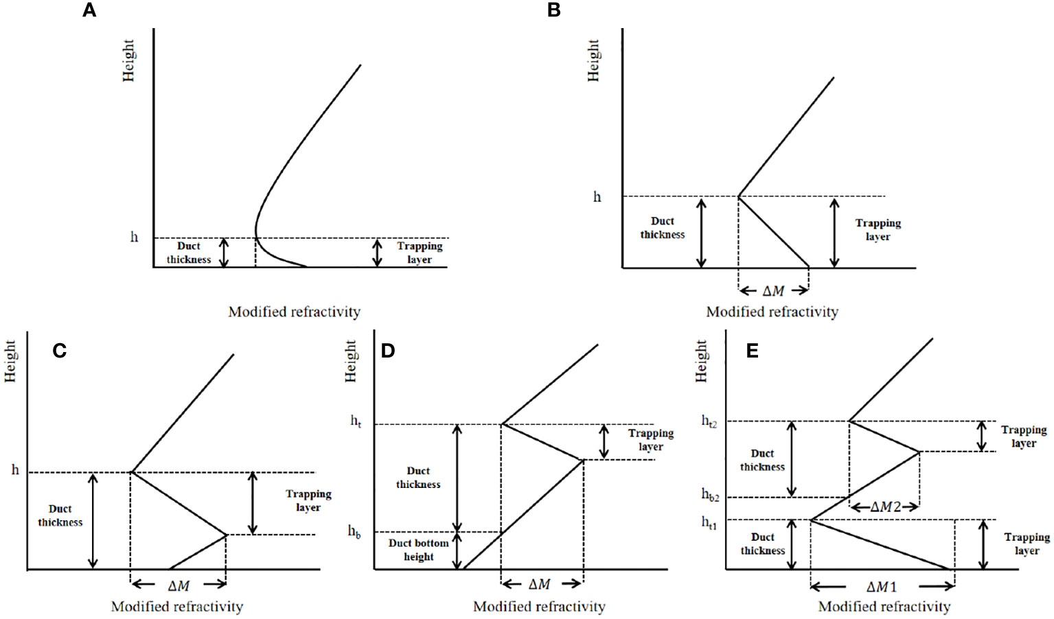
Figure 1 Lower atmospheric duct types: (A) evaporation duct, (B) simple surface duct, (C) surface-based duct, (D) elevated duct, (E) composite duct. The characteristic parameters of the duct were adapted from Turton et al., 1988.
It is worth noting that the height of the evaporation duct is mostly around 10~20 m, and the height rarely exceeds 40 m. It cannot be well captured by numerical models, so it is not considered in this study. The other four types of lower atmospheric ducts (Figures 1B–E) are adopted in the diagnosis scheme and their duct strength, thickness, and height parameters are diagnosed.
The strength of ducts in Figure 1 is denoted as ΔM, which represents the ability to trap electromagnetic waves and is defined as the difference in modified atmospheric refractivity between the top and bottom heights of the duct layer. The duct thickness is referred to as the height difference between the top and bottom of the duct layer. The top and bottom height of ducts, at which the modified atmospheric refractivity is equal in values, is defined as the maximal and minimal height of the duct layer based on the profile of the modified atmospheric refractivity (Turton et al., 1988). In this study, the duct characteristic parameters refer to the duct height, thickness, and intensity. For convenience, the duct height mentioned later is defined as the average value of the top and bottom heights of the ducts.
Figure 2 shows the flowchart for diagnosing lower atmospheric ducts. The specific diagnosis steps are listed as follows:

Figure 2 The flowchart for diagnosing lower atmospheric ducts.
a. Read the simulated temperature, humidity, height, and pressure variables from WRF, and calculate the modified atmospheric refractivity based on Equations (1)–(3).
b. After initialization, the gradient of modified atmospheric refractivity was checked at each layer. Once the gradient is satisfied by (Equation 4):
It is believed by Turton et al. (1988) that a trapping refraction phenomenon for electromagnetic waves appears and the atmospheric duct occurs. Then, search upwards for the difference in modified atmospheric refractivity values (ΔM) between the base and top of the duct, which represents the duct strength in Figure 1.
c. Check whether the diagnosed duct strength exceeds the set threshold. If not, it is considered as a minor disturbance and will not be output. If so, it is labeled as the first layer of duct, and then the type of duct is determined based on the profile shape.
d. Check whether the modified atmospheric refractivity at the duct top is less than or equal to the refractivity value at the lowest layer. If it is, it is a surface duct; if not, it is an elevated duct (Figure 1C). Next, check whether the modified atmospheric refractivity at the duct base is greater than the refractivity value at the lowest layer. If it is, it is a surface-based duct with a base layer (Figure 1B); if not, it is a simple surface duct close to the sea surface (Figure 1A).
e. Calculate the duct thickness, which is the height difference between the top and bottom of the duct. The average duct height is the average height value of the duct bottom and top.
f. Check whether the current height of the duct top is the maximum height. If not, enter the loop and continue diagnosing at higher altitudes. If it is, check if the marked number of duct layers is two. If not, the current duct is only a single-layer duct. If it is, the number of duct layers is two, and the second layer is always an elevated duct, labeled as a composite duct (Figure 1D). Since the occurrence of three-layer ducts is very rare, ducts with more than two layers are not displayed.
The sounding data used for validation in this work originated from three radiosonde stations at different latitudes. Particularly, the data were obtained from the University of Wyoming’s Global Upper Air Observational Database (http://weather.uwyo.edu/). The sounding balloons were released twice every day with an interval of 12 h. These sounding data provided valuable insights for various observation variables, such as air pressure, geopotential height, temperature, dew point temperature, relative humidity, specific humidity, wind direction, and wind speed. The sounding data at Kowloon station (ID: 45004, in Hong Kong), Baoshan (ID: 58362, in Shanghai) and Dalian (ID: 54662) during the year 2021 was utilized in the following evaluations. The locations of these stations were marked with red dots in Figure 3. In the data processing procedure, quality control was performed on the sounding data, following the standard methods for meteorological observational data processing. The control process included checks for the reasonability and mean values of temperature, humidity, and pressure, by adding conditional statements and flags to identify extreme data. The reasonability check primarily assessed whether each variable fell within the normal range of variation, while the mean value check examined if the values at a particular height deviated significantly from the average. After processing, these data were used to calculate the modified atmospheric refractivity using Equations (1)–(3), and then input into the diagnosis scheme in Section 2.2 to obtain the parameters of the lower atmospheric ducts. In the model validation process, the duct characteristic parameters obtained from sounding data were regarded as a reference for evaluation. Additionally, the ERA5 reanalysis data was used as the driving fields for the WRF model and also participated in some parts of validation works.
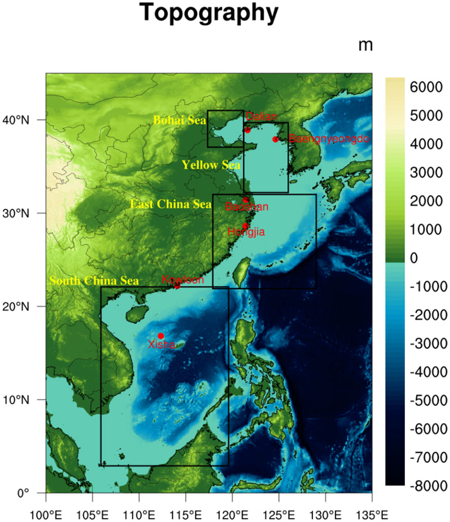
Figure 3 Topographic map over the domain of the WRF model in this work. The four areas framed by black lines are the typical areas chosen for the following statistical analysis. The locations of the sounding stations for validation are marked with red dots.
ERA5 is the fifth generation of reanalysis data of global climate and weather conducted by the ECMWF over the past eight years (https://www.ecmwf.int/en/forecasts/dataset/ecmwf-reanalysis-v5). It provides various atmospheric parameters at 37 pressure levels from 1000 hPa (approximately 70 m) to 1 hPa (approximately 48 km) in a temporal resolution of one hour and a horizontal resolution of 0.25° × 0.25°. When compared with the meteorological observations over China, the ERA5 data have demonstrated a high level of accuracy (Jiang et al., 2021; Wang Z. et al., 2023).
Before conducting the formal long-term simulations, two groups of sensitivity tests were conducted to guarantee the reasonability and accuracy of the long-term simulation results. First, to investigate the impacts of the error accumulation on the atmospheric ducts during the continuous simulations, four sensitivity tests (S1, S2, S3, and S4) with different durations of continuous integration simulations were conducted using the WRF model. More specifically, the S1 test represented a continuous integration for one month, the S2 test denoted an integration for 15 days followed by a restart and integration for another 15 days, and the S3 and S4 tests stated the integration durations of 10 days and 5 days, respectively. The simulations lasted for the whole month of August 2021 for all four tests, and the sounding data from the Dalian, Baoshan, and Kowloon stations was used for error evaluations. Table 1 presents the Root Mean Square Errors (RMSEs) of the modified atmospheric refractivity at three stations for the four tests. From our analysis, it was observed that as the time duration in a single continuous integration increased, its error tended to increase correspondingly at all the three stations. This increase in bias indicated a positive correlation between the integration time and the accumulated errors during the simulation processes. The mean bias in the test with integration of one month (S4) increased by 4.46% when compared with the S1 test with a duration of five days.
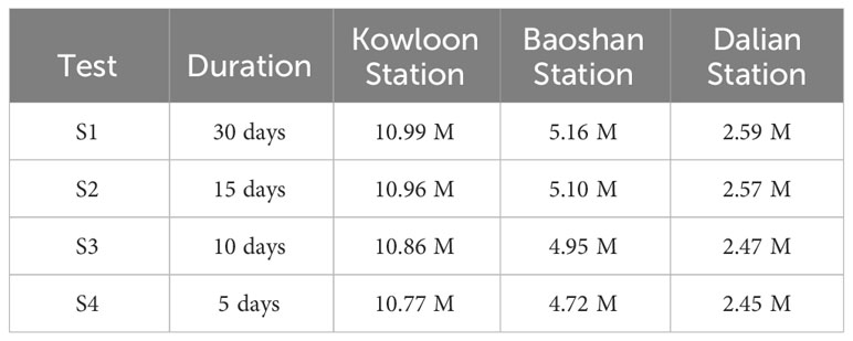
Table 1 Mean RMSEs of sensitivity tests for single simulation time duration.
Considering the convenience of practical operations, the following formal long-term simulation tests were conducted with a single simulation duration of 6 days, with the first day used as a spin-up period to reduce errors. It should be noted that the atmospheric duct events are separate events similar to typhoons, and the parameters of ducts are not continuous variables like air temperature. Therefore, this discontinuous way of integration simulation would not have a significant negative impact on the diagnosis of the atmospheric duct events.
Subsequently, to investigate the impact of the different nudging strategies on modeling error bias, eight groups of sensitivity tests (numbered from T1 to T8) on nudging methods were conducted. Essentially, the nudging method is a four-dimensional assimilation approach that regularly constrains the simulated results using the regional and boundary information from the forcing fields. According to the literature, it has been demonstrated that during long-term simulations, the nudging method can effectively reduce modeling errors (Liu et al., 2012; Gómez and Miguez-Macho, 2017; Kruse et al., 2022). In this work, the eight sensitivity tests lasted for one month and were conducted using different nudging strategies over the China seas. Table 2 presents the errors of the modified atmospheric refractivity from the eight tests nudged with different variables at different height levels using two nudging methods (grid nudging and spectral nudging). Overall, the T3 test using the grid nudging method provided the lowest RMSEs at the three stations. Therefore, the subsequent long-term simulations adopted the same nudging way of the T3 test as well.
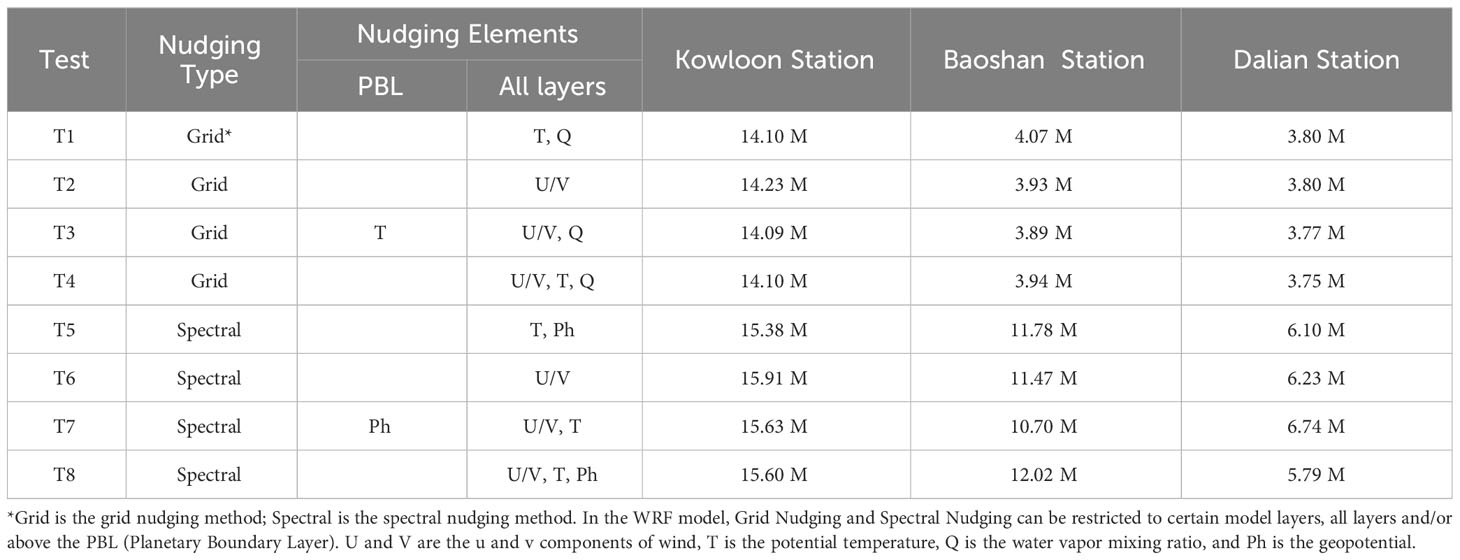
Table 2 Mean RMSEs of sensitivity tests with different nudging methods.
The China seas with its surrounding areas were chosen as the study domain. Figure 3 illustrates the topography over the domain. The red dots represent the locations of three sounding stations used for model validation. The WRF model was configured with grids of 300×350, in a horizontal resolution of 15 km and 45 vertical layers. The parameterization schemes employed in WRF were the WRF Single Moment 6 class (WSM6) microphysics scheme (Grasso et al., 2014), the Dudhia shortwave radiation scheme (Dudhia, 1989), the Rapid Radiative Transfer Model (RRTM) longwave radiation scheme (Mlawer et al., 1997), the MM5 surface layer scheme (Beljaars, 1995), the Unified Noah land surface model (Chen and Dudhia, 2001), the Yonsei University Scheme (YSU) planetary boundary layer scheme (Hong et al., 2006), and the Grell-Freitas ensemble cumulus convection scheme (Grell and Freitas, 2014). The nudging method was the way of the T3 test, which employed the grid nudging for temperature within the planetary boundary layer and for wind and humidity at all levels.
The WRF model was driven by the ERA5 reanalysis data, and the formal long-term test spanned from 00:00 UTC on December 31, 2010, to 00:00 UTC on January 1, 2022, covering a period of ten years. The model was continuously integrated for six days in each simulation, with the first day serving as a spin-up period and the subsequent five days used for actual analysis.
The ERA5 data was used as the driving data of WRF in this study. Specifically, based on the regional configuration of the WRF model, the pre-processing module (WPS) utilized ERA5 data to create initial and boundary condition files necessary for the WRF model operation. These files provided initial values to the WRF model and constrained the boundaries during model ran, ensuring the continuous operation of WRF. Therefore, the simulation results of WRF were essentially the dynamical downscaling products of ERA5 data, which had higher spatiotemporal resolutions. According to Equations (1)–(3), variables such as temperature, specific humidity, pressure, and height extracted from WRF simulation results were used to calculate the modified atmospheric refractivity and following duct diagnosis.
The sounding data during the year 2021 from the three radiosonde stations was used for evaluations. To demonstrate the climatological state of the atmosphere, Figure 4 presents the mean profiles of temperature, humidity, pressure, and modified atmospheric refractivity for the month of August 2021 as an illustrative example. As shown in the figure, with increasing altitude, the numerical values of temperature, humidity, and pressure progressively decreased, while the modified atmospheric refractivity gradually increased due to the consideration of altitude. The WRF results closely matched the sounding data, with only slight deviations observed in simulating humidity below 1000 meters and above 6000 meters. Overall, the WRF results exhibited slightly larger bias compared to ERA5 data below 1000 meters, but significantly lower bias above 6000 meters. Additionally, compared to the absolute values of modified atmospheric refractivity, the bias between WRF and observations was rather tiny and hard to be discerned in the figure, indicating a close agreement between the simulated and observed profiles.
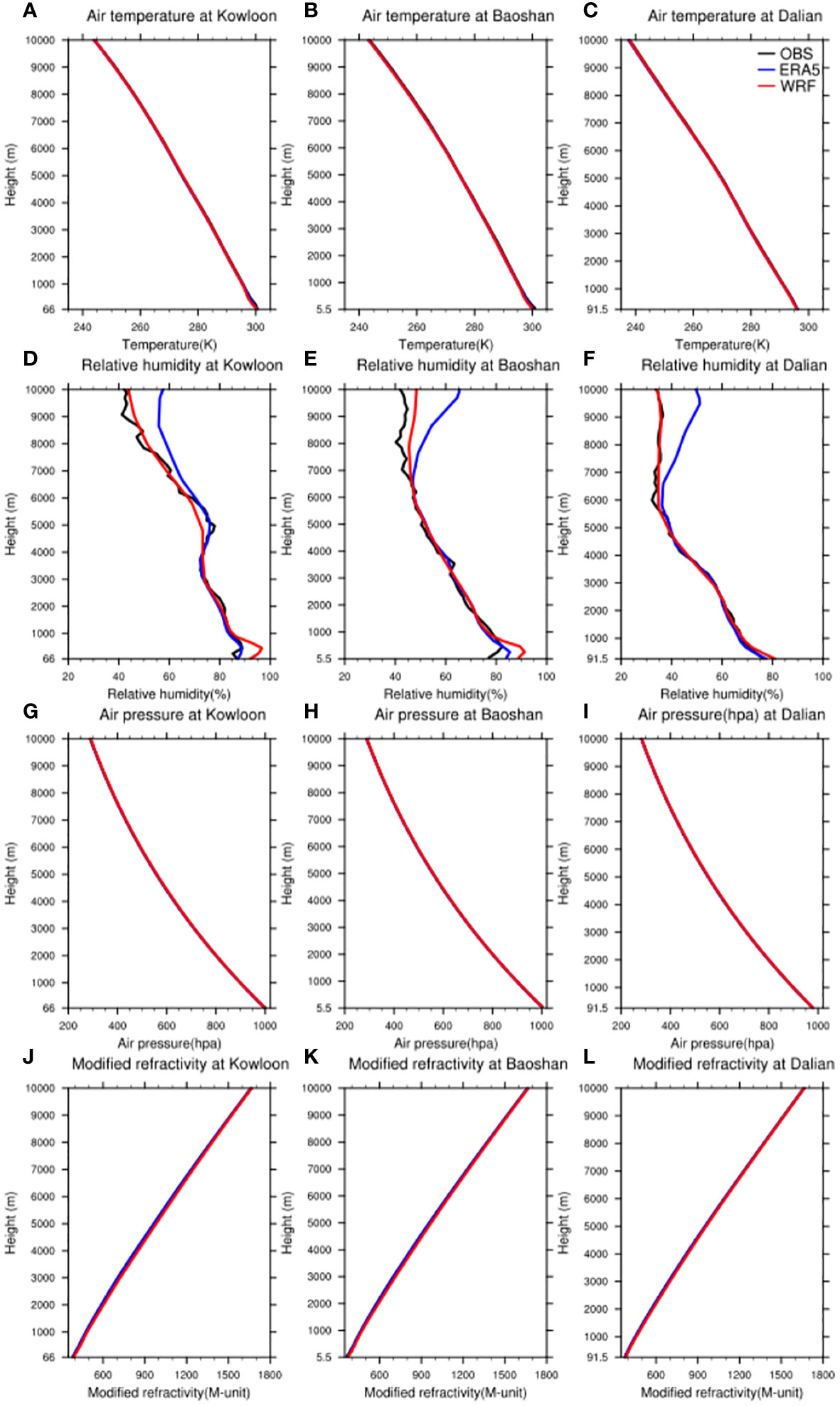
Figure 4 Monthly mean profiles of air temperature at (A) Kowloon Station, (B) Baoshan Station and (C) Dalian Station, relative humidity at (D) Kowloon Station, (E) Baoshan Station and (F) Dalian Station, air pressure at (G) Kowloon Station, (H) Baoshan Station and (I) Dalian Station, and modified atmospheric refractivity at (J) Kowloon Station, (K) Baoshan Station and (L) Dalian Station in August, 2021. The red, blue and black lines are denoted as the WRF results, ERA5 data and sounding observations, respectively.
Figure 5 depicts the vertical profiles of RMSEs and the correlation coefficients for the simulated modified atmospheric refractivity at the locations of three stations. Figures 5A–C illustrate the RMSE profiles at the Kowloon, Baoshan and Dalian stations, respectively. The ERA5 reanalysis data after interpolation also participated in the comparison process. As can be observed in the figure, the RMSE values of WRF (red lines) at the three stations remained within the range of 4 M to 7 M, with the mean values of 5.93 M, 4.8 M, and 4.67 M, respectively. Generally, there were no clear trends with height in the error profiles within the height range of 10000 m, indicating that the performance of WRF remained stable at all the height levels. As for the vertical variations, the RMSE of WRF changed by -0.10 M/km, -0.06 M/km, and -0.05 M/km, respectively. For comparison, the ERA5 data (blue lines) were generally closer to the sounding observations, with mean errors of 2.91 M, 3.38 M, and 2.97 M, respectively. The changing rates of RMSE with height were -0.39 M/km, -0.20 M/km, and -0.09 M/km, respectively, slightly larger than the WRF results.
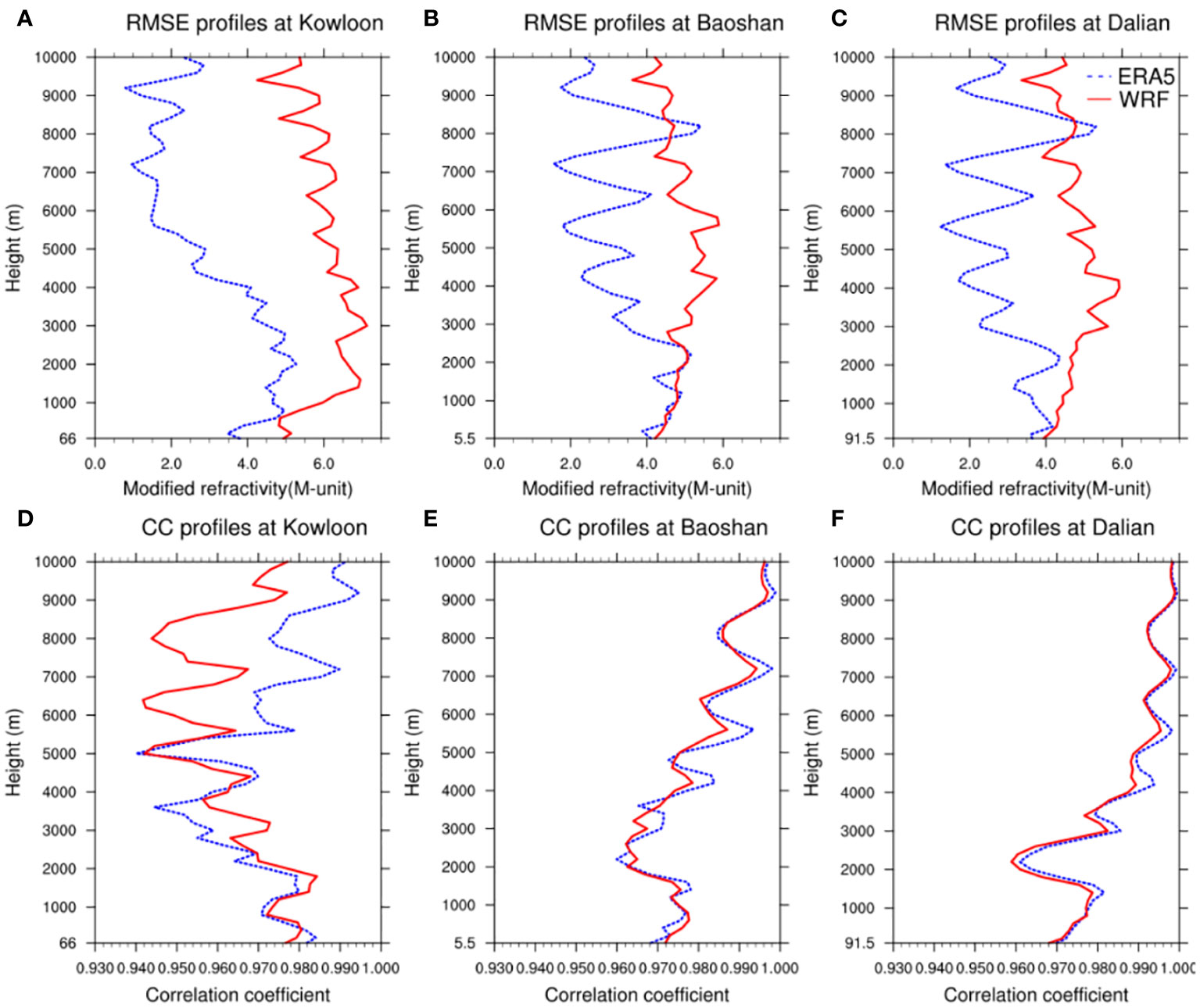
Figure 5 Mean Root-Mean-Square Error (RMSE) profiles of the modified atmospheric refractivity from the WRF simulations and ERA5 reanalysis data compared with the local sounding data at (A) Kowloon Station, (B) Baoshan Station and (C) Dalian Station, and the mean Correlation Coefficient (CC) profiles of the modified atmospheric refractivity from the WRF simulations and ERA5 reanalysis data compared with the local sounding data at (D) Kowloon Station, (E) Baoshan Station and (F) Dalian Station. The red lines are denoted as the WRF results and the blue dot lines as the ERA5 reanalysis data.
Figures 5D–F show the profiles of the correlation coefficients between the simulations and the sounding data at the three stations. Generally, the WRF simulations maintained a high level of correlation with the observations, with mean values of 0.96, 0.98 and 0.99, respectively. Similar to Figure 5A, the correlation coefficients at Kowloon station were slightly lower, with a weak decreasing trend as the altitude increased. However, the decreased degrees remained within 0.04 at the altitude of 10000 m. For the other two stations, the correlation coefficients gradually increased with altitude, with the values even exceeding 0.995 at an altitude of 10000 m. The changing rates of the correlation coefficient with height were -0.001/km, 0.003/km, and 0.003/km, respectively. The ERA5 data, as a comparison, were not obviously different from the simulations, with mean correlation coefficients of 0.97, 0.98, and 0.99. Its vertical changing rates were consistent with the WRF results, with values of 0.002/km, 0.003/km, and 0.003/km, respectively.
To enhance the credibility of model performance, three additional stations (including Xisha, Hongjia, and Baengnyeongdo) were also selected to calculate the RMSE and correlation coefficient of the WRF results. The locations of the stations were marked in Figure 3. The mean RMSE values of the WRF results at these three stations were 7.09 M, 6.39 M, and 6.27 M, respectively, with corresponding correlation coefficients of 0.85, 0.90, and 0.92. This level of error was comparable to that of other models. Haack et al. (2010) compared the performance of different numerical models in simulating modified atmospheric refractivity using profile observation data from the Wallops-2000 field program. The range of bias for all models was within 2.9 M to 15.7 M below 500 meters in height. Although the errors in modified atmospheric refractivity simulations by numerical modeling may have some negative impact on electromagnetic wave propagation simulation, it is not significant. The vertically drastic variation of refractivity or atmospheric duct phenomena are the main factors affecting the trajectory of electromagnetic wave propagation. This view was also demonstrated in the sensitivity analysis conducted by Pastore et al. (2021).
In brief, the WRF model demonstrated excellent performance in simulating the modified atmospheric refractivity and could be utilized for subsequent duct diagnostics.
As referred above, the RMSEs and correlation coefficients of WRF were slightly lower than those of ERA5 data in terms of modified atmospheric refractivity. However, the focus of this study is not modified atmospheric refractivity but the parameter characteristics of lower atmospheric ducts, which are based on further diagnostic data derived from modified atmospheric refractivity. The duct diagnostic ability of the WRF model was evaluated using the observations from the three radiosonde stations. Table 3 presents three technical indices of the diagnosed ducts including the hit rate, FAR (false alarm ratio) and CSI (critical success index) (Roebber, 2009). As shown in the table, the hit rates of ducts simulated by WRF remained at approximately 40~70% across three sounding stations, while the FARs were at the highest at only around 25%. These values were comparable to the benchmark performance of the MetUM (Met Office Unified Model) reported by Haack et al. (2010), and were higher than those of the MM5 and GEM (Global Environmental Multiscale) models. In contrast, all three indices of ERA5 data were considerably lower, and most atmospheric duct phenomena could not be diagnosed using ERA5 data. Generally, Table 3 indicated that WRF’s simulations had a high reliability in duct diagnosis, while it was hard for the ERA5 data to obtain sufficiently accurate results due to their limited vertical layers if without further treatments on the data.
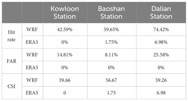
Table 3 Hit rate, FAR and CSI of ducts diagnosed from WRF and ERA5 data at sounding stations.
Based on the ten-year simulations using the WRF model, the spatial distributions of the lower atmospheric ducts over China seas were represented as follows. Figure 6 presents the spatial distributions of the occurrence rates of the four types of lower atmospheric ducts mentioned in Figure 1. Overall, all four types of ducts showed obvious regional characteristics. Among them, the simple surface ducts near the sea surface had the highest occurrence rates, with a mean occurrence rate of 41.97% over the domain. The composite ducts with two or more layers had a mean occurrence rate of 10.82%. The surface-based and elevated ducts were only detected in certain areas, with mean occurrence rates of 4.74% and 8.47%, respectively.
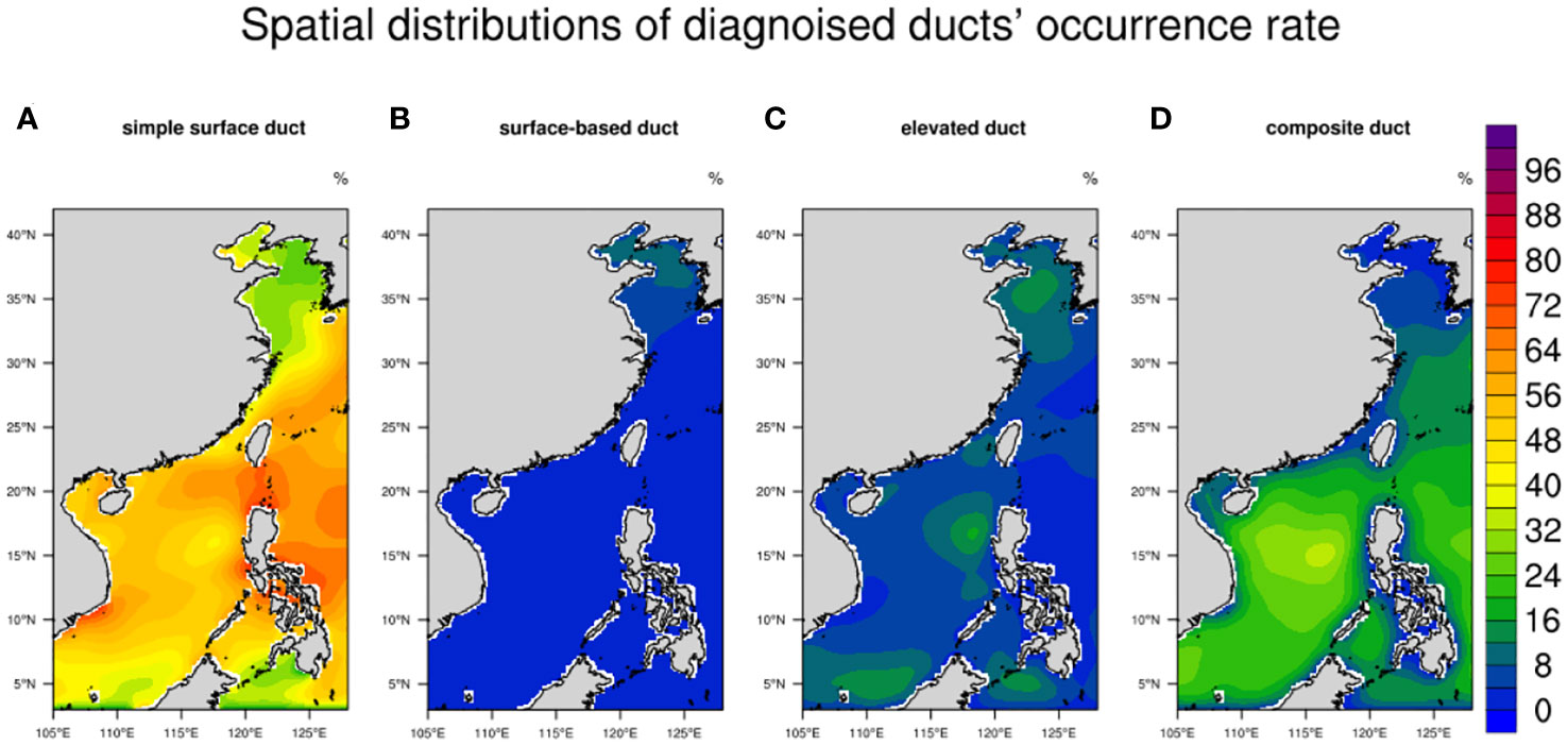
Figure 6 The spatial distributions of the diagnosed ducts’ occurrence rate of the (A) simple surface duct, (B) surface-based duct, (C) elevated duct, and (D) composite duct.
More specifically, Figure 6A presents the distribution of the occurrence rates of simple surface ducts. The trapping layers of this duct type lie above the sea surface, with the atmospheric refractivity index at the top of the duct layer being smaller than that at the sea surface. Its formation is related to the nocturnal radiative inversion of the temperature or the advection of dry and warm air in the lower atmosphere. The occurrence rates of this duct type were generally higher in low-latitude regions compared to mid-latitude regions. Additionally, the entire domain was further divided into four sea areas (Bohai Sea, Yellow Sea, East China Sea, and South China Sea) for separate local analysis, as framed by the black rectangular boxes in Figure 3. The highest occurrence rate was observed in the East China Sea (22°~32°N, 117°~128°E) with 52.87%, followed by the South China Sea (2°~22°N, 105°~119°E) with 50.88%. The lowest occurrence rate was found in the Yellow Sea (32°~39°N, 121°~126°E) with 29.88%, and the Bohai Sea (37°~41°N, 117.3°~121°E) had an occurrence rate of 34.23%.
Figure 6B displays the distribution of surface-based ducts with a base layer. These ducts are composed of a trapping layer overlaying on a sea-level base layer with a low gradient of refractivity index. In contrast to Figure 6A, the ducts of this type mostly occurred in mid-latitude regions including the Bohai Sea and Yellow Sea, with occurrence rates of 10.8% and 7.41%, respectively. They seldom occurred in the East China Sea and South China Sea, with occurrence rates of only 0.63% and 0.13%, respectively. Interestingly, the spatial distributions of the surface ducts of these two types showed certain complementary characteristics. When combining the distributions of Figures 6A, B, the occurrence rate of the total surface ducts in the Bohai Sea was 45.02%, which was not significantly different from that in the South China Sea with 51.01%. In addition, their spatial differences were reduced to some extent. Figure 6C shows the occurrence rates of single-layer elevated ducts, which are composed of a trapping layer overlaid on a base layer. The modified atmospheric refractivity at the top of the duct layers for elevated ducts was greater than that at the surface. Their formation is closely related to the weather activities. The occurrence rates of elevated ducts did not show any significant regional differences, with rates of 8.96%, 11.39%, 5.79%, and 7.72% for the Bohai Sea, Yellow Sea, East China Sea and South China Sea, respectively. As for the composite ducts shown in Figure 6D, their distributions of occurrence rate showed a decreasing pattern from south to north, similar to that in Figure 6A. Among the seas, the South China Sea with the lowest latitude had the highest probability of 21.79%. The occurrence rates in the Bohai Sea, Yellow Sea, and East China Sea were 3.34%, 5.33%, and 12.82%, respectively.
Furthermore, the occurrence distributions in Figure 6 appeared to be very similar to the distributions of the sea surface temperature (SST). When examining the spatial correlation coefficients between the occurrence rates of ducts and SST in the domain, it was found that the spatial correlation coefficient between the occurrence of simple surface ducts (Figure 6A) and SST reached up to 0.95, indicating that SST might play an important role in the local surface duct formation process. The correlation coefficient between the distribution of surface-based ducts and SST was only 0.24, suggesting a weaker relationship with SST for the surface-based ducts that were far from the sea surface. The elevated ducts and composite ducts, which were closely related to weather activities, also exhibited high correlations with SST, with the coefficients reaching 0.78 and 0.83, respectively.
Due to space limitations, a detailed analysis of the characteristic parameters for all four types of ducts cannot be provided here. Therefore, as described in Section 2.2, the lower atmospheric ducts were divided into two levels according to their level positions. For the first layer of ducts, they were still composed of four types of ducts, with the same proportions as the previous results. In contrast, all ducts in the second layer were derived from the composite duct type in the second layer. Figure 7 presents the spatial distributions of three parameters—duct height, thickness, and strength—for the lower ducts. The duct height is denoted as the medium value between the bottom and top heights of the ducts layer. In this work, the distributions of the parameters for ducts in the first and second layers were provided. According to Figure 7, it was evident that the duct characteristics showed significant variations in the meridional direction. As shown by the distribution of the first-layer duct features in Figures 7A–C, the ducts in northern mid-latitude areas of the domain showed higher heights, thicker layers, and greater strengths when compared to those in the lower latitudes. The distributions of second-layer ducts shown in Figures 7D–F showed the opposite situations. The ducts in the South China Sea had significantly higher heights, thicknesses, and strengths when compared to the ducts in other seas. Considering the occurrence rates of ducts in Figure 6, it could be inferred that the ducts with single layers occupied a larger proportion of the total ducts in the northern mid-latitude seas, and the characteristics of the first-layer ducts are stronger. On the other hand, the ducts with multiple layers relied on strong vertical atmospheric activities and occurred only in specific seasons or weather conditions in the mid-latitude region. They were relatively scarce and weaker in strength compared to the ducts in low-latitude warm seas.
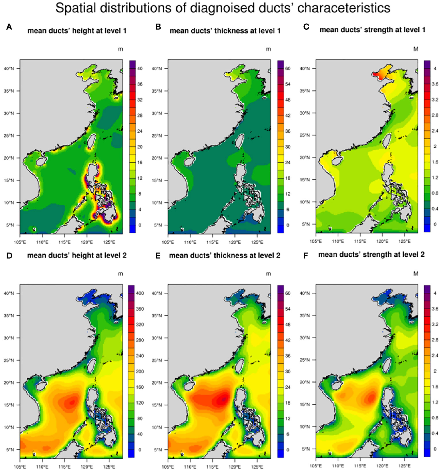
Figure 7 The spatial distributions of the diagnosed ducts’ characteristics of (A) mean ducts’ height at level 1, (B) mean ducts’ thickness at level 1, (C) mean ducts’ strength at level 1, (D) mean ducts’ height at level 2, (E) mean ducts’ thickness at level 2 and (F) mean ducts’ strength at level 2.
For each duct parameter, Figures 7A, D show the distributions of the mean heights for the ducts of two layers. The mean height of ducts at the first layer ducts was 8.12 m, with the highest value observed in the Bohai Sea and the lowest value in the South China Sea. The ducts at the second layer had a mean height of 97.78 m, showing significant spatial variations compared to the height of the first layer. The highest value of 223.91 m was observed in the South China Sea, while the lowest value was only 20.88 m in the Bohai Sea. Figures 7B, E illustrate the distributions of duct thickness for the ducts of two layers, which resembled the patterns in Figures 7A, D. The mean thickness over the entire domain was approximately 10.99 m and 18.36 m for the ducts at the first and second layers, respectively. A positive correlation between the duct height and thickness was observed. Figures 7C, F depict the distributions of duct strength. The mean strength of ducts at the first layer was 1.6 M over the domain, with the highest values concentrated in the Bohai Sea, reaching up to 58.44 M. The mean strength at the second layer was 0.87 M over the domain because of the low strength in the seas to the north of the South China Sea. The highest value was found in the northern part of the South China Sea, reaching up to 58.23 M. The existence of higher duct strengths indicated that a wider spectrum of electromagnetic waves could be trapped, resulting in more significant impacts on radio communication. Therefore, atmospheric ducts should be given greater attention, in terms of their influence on wireless communication in the Bohai Sea and northern areas of the South China Sea.
In addition to the above-mentioned climatological analysis, the seasonal variations of lower duct characteristics at different seas were also investigated. The duct parameters averaged over the four sea areas will be presented to illustrate the monthly variations.
Figure 8 illustrates the monthly variations of the occurrence rates of the ducts of four types in the four sea areas. For convenience, the occurrence rates of ducts of the four types were accumulated using different colors on the same column. As shown in Figure 8, the duct occurrence rates in all seas presented a seasonal distribution with two peak values, and the seasons of peak occurrences differed with latitudes. For the Bohai Sea and Yellow Sea in the mid-latitudes, the first peak of high occurrences appeared in spring, when the ducts of four types occurred with similar occurrence rates. The second peak occurred in autumn, with higher values than that in spring and most of them being simple surface ducts near the sea surface. For the South China Sea in the low-latitudes, the two peaks occurred in early summer and early winter, about two months later than those in the Bohai Sea and Yellow Sea. The monthly distributions of duct occurrence in the Yellow Sea were very similar to the conclusions of Tang et al. (2008) based on the sounding data. During April and May, the transition period of monsoons, the water vapor content at lower levels increased with the temperature rising, resulting in an increase in duct occurrence and the formation of the first peak. In July and August, owing to the northward movements of the subtropical high pressure system, the vertical humidity gradient decreased, which was not favorable for duct formation, and therefore the duct occurrence rates decreased. In autumn, the Yellow Sea was controlled by weaker cold high pressures, with sufficient water vapor at lower levels. The atmosphere at upper levels was controlled by the westerly belt with lower humidity, and large humidity gradients were formed with frequent inversions in temperature, which resulted in the highest rates of duct occurrence in a year. Later, as the cold high-pressure system further strengthened in winter and the temperature and water vapor decreased, the duct occurrence also correspondingly decreased.
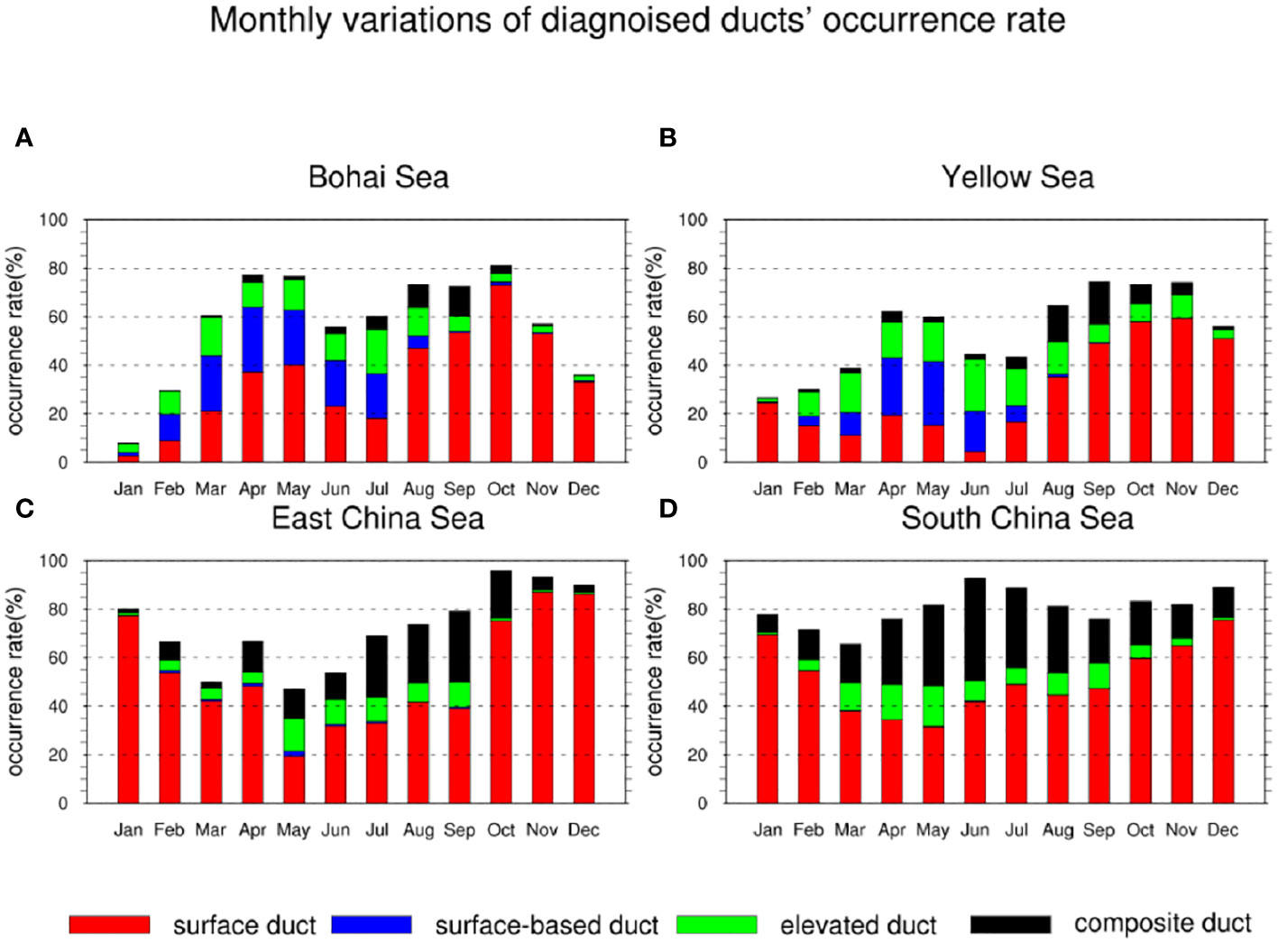
Figure 8 Monthly variations of the diagnosed ducts’ occurrence rate over the (A) Bohai Sea, (B) Yellow Sea, (C) East China Sea, and (D) South China Sea. The red columns indicate the rates of simple surface ducts; the blue columns indicate the rates of surface-based ducts; the green columns indicate the rates of elevated ducts and the black columns indicate the rates of composite ducts.
The seasonal distributions of ducts in the East China Sea were like the transition from the South China Sea to the Yellow Sea, with comparable proportions of duct types as those in the South China Sea. However, the seasonal differences are more similar to the duct characteristics in the Yellow Sea. For the seasonal differences, the seasons when most ducts occurred were not summer and winter, which were controlled by prevailing warm and cold air masses. Although local convection and tropical cyclone activities were more active in summer, they appeared not to be the main causes of duct formation, which was consistent with the findings of Basha et al. (2013) based on observational statistics. According to the seasonal distributions depicted in Figure 7, duct occurred more frequently during the transition seasons between winter and summer monsoon seasons, which took place in spring and autumn. Therefore, the dominant factors influencing the frequency of duct occurrences were likely the combined effects of sea surface temperature changes and the convergence of large-scale warm and cold air masses associated with the monsoon process. It is also worth noting that the seasonal variations of ducts in the East China Sea and the South China Sea were found highly related to the occurrence frequency of cold air processes, according to the statistics by Zhu et al. (2022) over this area. Due to the space limits in this work, the relationships between the intense cold air activities and temporal variations of atmospheric ducts will be further investigated in future research, as Figure 8 contains many interesting climate-related topics worthy of further exploration.
In terms of the duct of each type, simple surface ducts (red bars) accounted for a large proportion of the total occurrence rates, and this proportion reached its maximum in autumn and winter. This effect might result from situations in which the temperature decreased with the gradually stabilized atmospheric stratifications but the temperature at the underlying sea surface still remained warm. In spring and summer, the proportions of simple surface ducts decreased due to the occurrence of ducts of other types. The surface-based ducts (blue bars) mostly occurred in the Bohai Sea and Yellow Sea at mid-latitudes, and their occurrences were concentrated in spring with rare occurrences in other seasons (Figures 8A, B). For this special distribution, it is doubted that it was related to warm air activities over colder water surfaces, which was unusual in other seasons and seas. The single-layer elevated ducts (green bars) were concentrated in spring and summer and accounted for a small proportion of all ducts at all seas. The occurrence rates of multi-layer composite ducts (black bars) in low-latitudes were apparently higher than those in mid-latitudes. In the Bohai Sea, Yellow Sea, and East China Sea, they mostly occurred in July, August, and September, which appeared to be closely related to local convection, cyclones, and other activities. In the South China Sea at low latitudes, high occurrence rates throughout the summer half year (from the spring equinox to the autumn equinox) were detected.
In addition to the occurrence rates of ducts, Figures 9–11 show the monthly variations of three parameters including average height, thickness, and strength of ducts at four seas. The black dashed line represents the duct parameters at the first layer, while the red solid line represents the ones at the second layer.
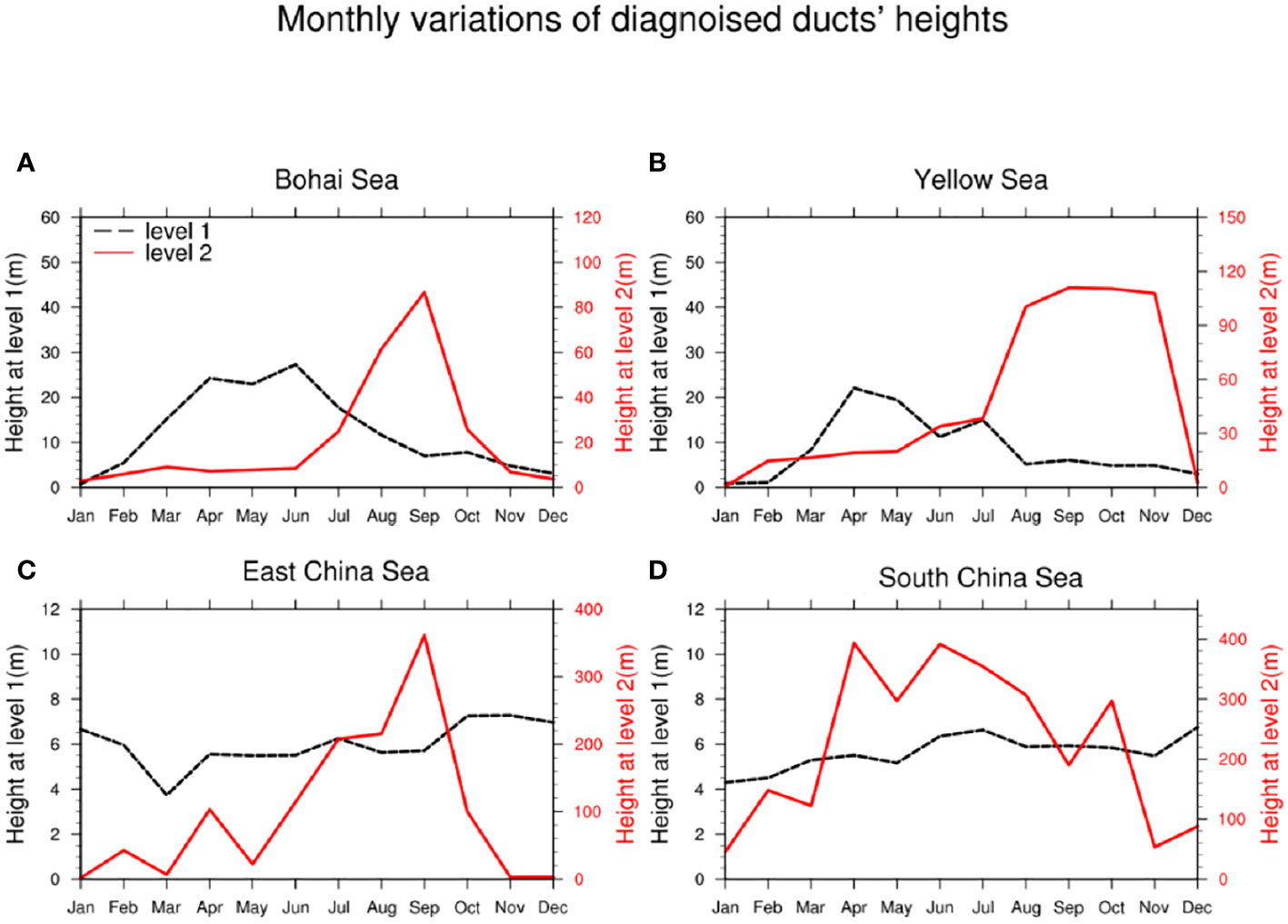
Figure 9 Monthly variations of the diagnosed ducts’ heights over the (A) Bohai Sea, (B) Yellow Sea, (C) East China Sea, and (D) South China Sea. The black dashed lines indicate the heights at level 1; the red lines indicate the heights at level 2.
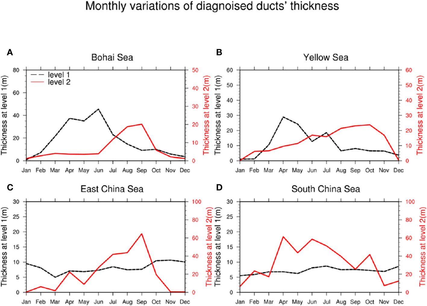
Figure 10 Monthly variations of the diagnosed ducts’ thickness over the (A) Bohai Sea, (B) Yellow Sea, (C) East China Sea, and (D) South China Sea. The black dashed lines indicate the thickness at level 1; the red lines indicate the thickness at level 2.
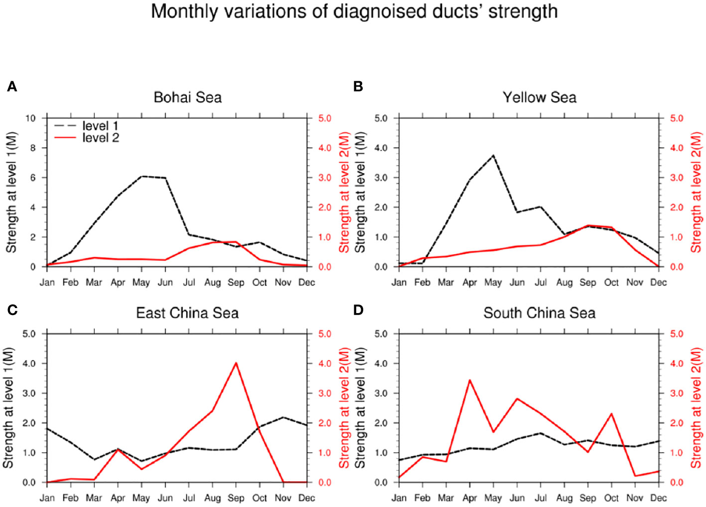
Figure 11 Monthly variations of the diagnosed ducts’ strength over the (A) Bohai Sea, (B) Yellow Sea, (C) East China Sea, and (D) South China Sea. The black dashed lines indicate the strength at level 1; the red lines indicate the strength at level 2.
According to Figures 9–11, there was a strong consistency in the monthly variations of height, thickness, and strength characteristics of the ducts. In the Bohai Sea and Yellow Sea of mid-latitudes, single-layer ducts occupied most proportions of the total ducts. The ducts at the first layer showed higher heights, greater thickness, and stronger strengths compared to those in the lower latitudes. The variations of ducts at the second layer showed the opposite distributions, with a lower occurrence of composite ducts in the Bohai Sea and Yellow Sea (as shown in Figure 6D) and weaker characteristics parameters compared to those in the southern low-latitude seas. As far as the duct height shown in Figure 9 is concerned, the seasonal variations of ducts at the two layers were completely different. In the Bohai Sea and Yellow Sea, the duct height at the first layer reached its peak in spring, while the monthly variations of the duct height at the second layer were consistent with the seasonal variations of composite ducts shown in Figure 8. The peak occurred in autumn, which was also the season with the highest occurrence of composite ducts.
In the East China Sea and South China Sea, the ducts at the first layer were mainly surface ducts that persisted throughout the year, with stable distributions of duct height without significant monthly variations. In the South China Sea at low latitudes, the duct height at the second layer remained relatively high throughout the year except in winter.
Figures 10 and 11 showed similar monthly variations with Figure 9. In the Bohai Sea and Yellow Sea, the peaks of duct thickness and strength at the first-layer duct were significantly higher than those in the South China Sea, with more significant seasonal variations. The duct thickness and strength at the second layer in the Bohai Sea and Yellow Sea region were significantly weaker than those in the South China Sea. As a transitional zone, the duct characteristics at the first layer in the East China Sea were similar to that in the South China Sea, while the seasonal variations at the second layer presented the single-peak pattern in autumn as observed in the Bohai Sea and Yellow Sea.
In this work, a diagnostic model of lower atmospheric ducts was developed based on the WRF model to obtain the characteristics of lower atmospheric ducts of different types. Using this diagnostic model, a strategy for long-term simulations was confirmed based on multiple sensitivity tests conducted earlier. Subsequently, a ten-year simulation test was conducted over the China seas. The ERA5 reanalysis data were utilized as the driving field, and the sounding data served as the benchmark for evaluations. By analyzing the simulated results, the spatiotemporal variations in the characteristics of lower atmospheric ducts were investigated over the China seas. The specific conclusions are presented below.
(1) Compared with the sounding data from Kowloon, Baoshan, and Dalian stations in the year 2021, the simulated modified atmospheric refractivity dataset generated in this study had a high accuracy. The simulated RMSEs of the modified atmospheric refractivity remained between 4 M and 7 M, and there were no significant changing trends with altitude. The error level was slightly higher than that of ERA5 reanalysis data, which was between 2.91 M and 3.38 M. In addition, the simulated results had a very high temporal correlation with the sounding data, with an average correlation coefficient of over 0.96.
(2) The characteristics of the lower atmospheric duct obtained based on the diagnostic model in this work also showed high reliability and could provide more accurate atmospheric duct information compared to the diagnosed results using the ERA5 data. The validation results based on the sounding data indicated that the dataset of atmospheric duct characteristics produced in this work slightly underestimated the duct occurrence rates but significantly outperformed the vertically lower-resolution ERA5 data. This underestimation might be attributed to the smoothing of the vertical variations in the model, which was a common issue in numerical models and could not fully reproduce the small-scale instantaneous fluctuations and stochastic oscillations observed in sounding data.
(3) Based on the analysis of the long-term duct dataset generated in this work, significant regional variations were observed in the duct occurrence rates at China seas. The simple surface ducts near the sea surface showed the highest occurrence rate, followed by the composite ducts with two or more layers. The surface-based ducts with a base layer and elevated ducts only occurred in certain sea areas, with lower occurrence over the whole domain. More specifically, for the duct of each type, simple surface ducts primarily occurred in low-latitude areas, with much higher occurrence rates in the East China Sea and South China Sea than in the Yellow Sea and Bohai Sea. Most surface-based ducts occurred in the Bohai Sea and Yellow Sea. The spatial distributions of these two types of surface ducts showed complementarity, and only by combining the distributions of the two types, the regional differences in the occurrence rates were not significant across from middle latitudes to low latitudes. The occurrence rates of single-layer elevated ducts were relatively low, with slightly higher occurrences in the Bohai Sea and Yellow Sea. The composite ducts occurred most frequently in the South China Sea, with a distribution of occurrence rates that decreased from south to north. Additionally, SST played an important role in the formation of ducts, yielding a high correlation coefficient between its spatial distributions and the occurrence rate distributions of ducts.
(4) The height, thickness, and strength of ducts showed significant longitudinal differences. In the mid-latitude region of northern China, single-layer ducts were dominant, with stronger parameters in duct height, thickness, and strength at the first layer. However, multi-layer ducts mainly occurred in specific seasons and weather conditions, and their occurrence times were relatively less with weaker features. In the South China Sea of low latitudes, the duct characteristics were just the opposite. The ducts with two layers showed a high frequency of occurrence, with significantly stronger features at the second layer than at the first layer. There was generally a positive correlation with each other among the distributions of the duct height, thickness, and strength, which indicates that when a duct had a higher height it tended to be thicker and stronger.
(5) The seasonal variations of ducts in the four sea areas reveal that the occurrence rates of ducts in all sea areas showed a bimodal distribution, and there were significant differences among the ducts of the different types in different sea areas. More specifically, simple surface ducts accounted for the largest proportion of total occurrences, and they occurred most frequently in autumn and winter. The surface-based ducts mainly occurred in the Bohai Sea and Yellow Sea during spring. The single-layer elevated ducts mostly occurred in the spring and summer, and they accounted for a relatively small proportion of all the ducts in all sea areas. The multi-layer composite ducts exhibited a higher occurrence rate in low-latitude regions, especially in the South China Sea area, where they occurred frequently throughout the summer half-year.
(6) The seasonal variations of the duct height, thickness, and strength also showed a strong consistency. In the Bohai Sea and Yellow Sea, the ducts at the first layer showed the strongest features during spring, while the peak of the duct parameters at the second layer occurred in autumn, which was roughly in agreement with the seasonal variation of composite ducts. The ducts at the first layer in the East China Sea and South China Sea were mostly simple surface ducts that existed throughout the year, and their seasonal variation amplitudes were rather small. The seasonal variations of the ducts at the second layer in the East China Sea still retained the characteristic of the single-peak shape in autumn as observed in the Yellow and Bohai Sea, while the ducts’ characteristics at the second layer in the South China Sea remain relatively strong in most seasons except in winter.
It should be also noted that there are limitations and uncertainties in the simulation results of this study, which need to be further improved in the future. First, due to the space constraints, only a preliminary analysis of the climatological distributions and multi-year mean monthly variations of duct characteristics was conducted. Diurnal and inter-annual variations were not involved, and deeper mechanism analysis was also not provided. In addition, the spatio-temporal changes in the occurrence rates of ducts of four types were only analyzed and their parameters, such as height, thickness, and strength, for each type of duct were not further examined. In the subsequent work, long-term simulation results will be used to further analyze the parameter changes of each duct type and to conduct statistical and more in-depth mechanism analyses on events, such as the winter and summer monsoons, subtropical high activities, typhoons, etc.
Second, the validation of the proposed model was conducted only at three stations, and the validation results also had some randomness. Although in the main text, the modified atmospheric refractivity was assessed, in fact, the temperature and humidity RMSE at the three stations were also validated. The RMSEs of temperature were 0.86 K at Kowloon, 1.05 K at Baoshan, and 0.96 K at Dalian. The RMSEs of relative humidity were 11.38% at Kowloon, 12.67% at Baoshan, and 11.87% at Dalian. The simulated errors of temperature and humidity remained at low levels. In this study, the selection of the Kowloon, Baoshan, and Dalian stations was based on their representation of different sea areas from south to north and their relatively high station grades, which provide a wealth of data beneficial for ducting diagnostics. However, as these three stations are all located in the marginal areas of the South China Sea, East China Sea, and Yellow Sea. To enhance the credibility of the validation results, three additional stations (Xisha, Hongjia, and Baengnyeongdo) with abundant data were chosen. From the performance of the WRF results at these three stations, it is evident that the RMSE and correlation coefficients did not exhibit significant changes, indicating the WRF model’s ability to maintain stable regional simulation accuracy. Nevertheless, these efforts are not sufficient, in the future, data from more stations will be incorporated to conduct a more comprehensive validation of the simulation results against a wider range of variables.
Third, there are still certain discrepancies between the simulated atmospheric duct results in WRF and the actual conditions. Huang et al. (2022) statistically analyzed the occurrence probability of lower atmospheric ducts based on years of radiosonde data in the Yellow Sea region. According to their statistics, the probability of lower atmospheric ducts’ occurrence at Dalian station was approximately 20%, with a surface duct occurrence probability of about 4% and an elevated duct occurrence probability of about 16%. These results indicated a lower probability of ducts compared to the simulated duct probabilities in our study. There are several main reasons that may contribute to this inconsistency. The first reason is the resolution of the radiosonde data products. In other words, if with more observations below 300 meters, more duct occurrences were believed to be discovered. Also, there is a large height interval sometimes between the lowest one or two layers of the sounding data, which may be related to the initial stage of GPS positioning or signal transmission and reception processes, making it very unfavorable for the diagnosis of simple surface ducts near the surface. The second reason is the timing of the observations. Radiosonde data is only available at 00:00 UTC and 12:00 UTC. There is significant uncertainty as to whether the average probabilities at these two times can represent the daily average. After all, for the Chinese seas, these two observation times miss the most active period of weather in a day. The third reason is the inherent errors in the WRF simulations, and the simulated duct occurrences differ from the radiosonde observations to a certain extent. The fourth reason is that each duct diagnosis algorithm may have some inconsistencies for different studies, such as differences in diagnostic approaches, procedures, and threshold settings, which can lead to differences in results. These reasons collectively contribute to the uncertainties between the results presented in this study and the actual conditions. Finally, the mesoscale weather models use the same local parameterization schemes over the domain. If the domain covers a large area, the same local schemes may lead to error increase in some areas. Some climate models, such as the Regional Climate Model (RegCM), attempt to use different parameterization schemes in different latitudes of the simulation domain. In our future climate simulations using WRF, it is planned to conduct similar studies. Additionally, since the WRF weather model does not consider the dynamic feedback processes of the underlying sea surface, the lack of an ocean model may weaken the impact of oceans when studying the relationship between the maritime atmospheric ducts and climate change. Thus, in the future, coupled atmosphere-ocean models should be used to conduct more comprehensive simulations with more complete physical processes to make the results more objective and comprehensive.
The raw data supporting the conclusions of this article will be made available by the authors, without undue reservation.
QL: Formal Analysis, Writing – original draft. XZ: Methodology, Software, Supervision, Writing – review & editing. JZ: Writing – review & editing, Investigation, Conceptualization, Formal Analysis, Validation, Writing – original draft. TH: Writing – review & editing, Methodology. ZQ: Writing – review & editing, Data curation. BW: Writing – review & editing, Resources. ZL: Resources, Writing – review & editing. CC: Writing – original draft, Conceptualization, Investigation. RC: Writing – review & editing, Resources.
The author(s) declare financial support was received for the research, authorship, and/or publication of this article. This study was financially supported by the Key R&D Program of Shandong Province, China (2023ZLYS01), the National Natural Science Foundation of China (Grant nos. 42076195, 42206188, 42206001, 42176185), the Natural Science Foundation of Shandong province, China (Grant nos. ZR2022MD100, ZR2021MD114), the “Four Projects” of computer science (2021JC02002) and the basic research foundation (2023PY004, 2023PY050, 2023JBZ02) in Qilu University of Technology.
The authors declare that the research was conducted in the absence of any commercial or financial relationships that could be construed as a potential conflict of interest.
All claims expressed in this article are solely those of the authors and do not necessarily represent those of their affiliated organizations, or those of the publisher, the editors and the reviewers. Any product that may be evaluated in this article, or claim that may be made by its manufacturer, is not guaranteed or endorsed by the publisher.
Anderson K. D. (1995). Radar detection of low-altitude targets in a maritime environment. IEEE Trans. Antennas. Propag. 43, 609–613. doi: 10.1109/8.387177
Atkinson B. W., Li J.-G., Plant R. S. (2001). Numerical modeling of the propagation environment in the atmospheric boundary layer over the persian gulf. J. Appl. Meteorol. Clim. 40, 586–603. doi: 10.1175/1520-0450(2001)040<0586:NMOTPE>2.0.CO;2
Atkinson B. W., Zhu M. (2006). Coastal effects on radar propagation in atmospheric ducting conditions. Meteorol. Appl. 13, 53–62. doi: 10.1017/S1350482705001970
Babin S. M. (1996). Surface duct height distributions for wallops island, Virginia 1985-1994. J. Appl. Meteor. Climatol. 35, 86–93. doi: 10.1175/1520-0450(1996)035<0086:SDHDFW>2.0.CO;2
Babin S. M., Dockery G. D. (2002). LKB-based evaporation duct model comparison with buoy data. J. Appl. Meteorol. Clim. 41, 434–446. doi: 10.1175/1520-0450(2002)041<0434:LBEDMC>2.0.CO;2
Babin S. M., Young G. S., Carton J. A. (1997). A new model of the oceanic evaporation duct. J. Appl. Meteor. Climatol. 36, 193–204. doi: 10.1175/1520-0450(1997)036<0193:ANMOTO>2.0.CO;2
Basha G., Venkat Ratnam M., Manjula G., Chandra Sekhar A. V. (2013). Anomalous propagation conditions observed over a tropical station using high-resolution GPS radiosonde observations. Radio. Sci. 48, 42–49. doi: 10.1002/rds.20012
Battan L. J. (1973). Radar Observation of the Atmosphere (Chicago: University of Chicago Press), 324. doi: 10.1002/qj.49709942229
Bech J., Codina B., Lorente J., Bebbington D. (2002). “Monthly and daily variations of radar anomalous propagation conditions: How “normal” is normal propagation? In: Proc. Second European Conf. of Radar Meteorology (Delft, Netherlands: ERAD), 35–39. doi: 10.1083/jcb.145.3.437
Bech J., Sairouni A., Codina B., Lorente J., Bebbington D. (2000). Weather radar anaprop conditions at a mediterranean coastal site. Phys. Chem. Earth Pt. B-Hydrol. Oceans. Atmos. 25, 829–832. doi: 10.1016/S1464-1909(00)00110-6
Beljaars A. C. M. (1995). The parametrization of surface fluxes in large-scale models under free convection. Q. J. R. Meteorolog. Soc 121, 255–270. doi: 10.1002/qj.49712152203
Brooks I. M., Goroch A. K., Rogers D. P. (1999). Observations of strong surface radar ducts over the persian gulf. J. Appl. Meteorol. 38, 1293–1310. doi: 10.1175/1520-0450(1999)038<1293:OOSSRD>2.0.CO;2
Brunetti M., Vérard C. (2018). How to reduce long-term drift in present-day and deep-time simulations? Clim. Dyn. 50, 4425–4436. doi: 10.1007/s00382-017-3883-7
Burk S. D., Thompson W. T. (1997). Mesoscale modeling of summertime refractive conditions in the southern california bight. J. Appl. Meteorol. Climatol. 36, 22–31. doi: 10.1175/1520-0450(1997)036<0022:MMOSRC>2.0.CO;2
Chen F., Dudhia J. (2001). Coupling an advanced land surface–hydrology model with the penn state–NCAR MM5 modeling system. Part I: Model Implementation and Sensitivity. Mon. Weather. Rev. 129, 569–585. doi: 10.1175/1520-0493(2001)129<0569:CAALSH>2.0.CO;2
Cheng Y., Zhou S., Wang D., Lu Y., Huang K., Yao J., et al. (2016). Observed characteristics of atmospheric ducts over the South China Sea in autumn. Chin. J. Ocean. Limnol. 34, 619–628. doi: 10.1007/s00343-016-4275-2
Craig K. H., Hayton T. G. (1995). Climatic mapping of refractivity parameters from radiosonde data. AGARD. Conf. Proc., 1–43.
Craig K. H., Levy M. F. (1991). “Parabolic equation modelling of the effects of multipath and ducting on radar systems,” in IEE proc. Part F Radar signal process. (IET Digital Library) 138, 153–162. doi: 10.1049/ip-f-2.1991.0021
Crane R. (2003). Propagation Handbook for Wireless Communication System Design. CRC press. doi: 10.1201/9780203506776
Dinc E., Akan O. B. (2014). Beyond-line-of-sight communications with ducting layer. IEEE Commun. Mag. 52, 37–43. doi: 10.1109/MCOM.2014.6917399
Ding J., Fei J., Huang X., Cheng X., Hu X. (2013). Observational occurrence of tropical cyclone ducts from GPS dropsonde data. J. Appl. Meteorol. Clim. 52, 1221–1236. doi: 10.1175/JAMC-D-11-0256.1
Dudhia J. (1989). Numerical study of convection observed during the winter monsoon experiment using a mesoscale two-dimensional model. J. Atmospheric. Sci. 46, 3077–3107. doi: 10.1175/1520-0469(1989)046<3077:NSOCOD>2.0.CO;2
Emmanuel I., Adeyemi B., Ogolo E. O., Adediji A. T. (2017). Characteristics of the anomalous refractive conditions in Nigeria. J. Atmos. Sol. Terr. Phys. 164, 215–221. doi: 10.1016/j.jastp.2017.08.023
Frederickson P. A., Murphree J. T., Twigg K., Barrios A. (2008). A modern global evaporation duct climatology. Proc. Int. Conf. Radar., 292–296. doi: 10.1109/RADAR.2008.4653934
Gómez B., Miguez-Macho G. (2017). The impact of wave number selection and spin-up time in spectral nudging. Q. J. R. Meteorolog. Soc 143, 1772–1786. doi: 10.1002/qj.3032
Grasso L., Lindsey D. T., Lim K.-S. S., Clark A., Bikos D., Dembek S. R. (2014). Evaluation of and suggested improvements to the WSM6 microphysics in WRF-ARW using synthetic and observed GOES-13 imagery. Mon. Wea. Rev. 142, 3635–3650. doi: 10.1175/MWR-D-14-00005.1
Grell G. A., Freitas S. R. (2014). A scale and aerosol aware stochastic convective parameterization for weather and air quality modeling. Atmos. Chem. Phys. 14, 5233–5250. doi: 10.5194/acp-14-5233-2014
Haack T., Wang C., Garrett S., Glazer A., Mailhot J., Marshall R. (2010). Mesoscale modeling of boundary layer refractivity and atmospheric ducting. J. Appl. Meteorol. Clim. 49, 2437–2457. doi: 10.1175/2010JAMC2415.1
Hao X., Li Q., Guo L., Lin L., Ding Z., Zhao Z., et al. (2022). Digital maps of atmospheric refractivity and atmospheric ducts based on a meteorological observation datasets. IEEE Trans. Antennas. Propag. 70, 2873–2883. doi: 10.1109/TAP.2021.3098582
Hitney H. V., Richter J. H., Pappert R. A., Anderson K. D., Baumgartner G. B. Jr (1985). Tropospheric radio propagation assessment. P. IEEE 73, 265–283. doi: 10.1109/PROC.1985.13138
Hong S. Y., Noh Y., Dudhia J. (2006). A new vertical diffusion package with an explicit treatment of entrainment processes. Mon. Wea. Rev. 134, 2318–2341. doi: 10.1175/MWR3199.1
Huang L., Liu C., Jiang M. B. (2022). Statistical analysis of the occurrence probability and the characteristics of the lower atmospheric ducts in the Yellow Sea. Chin. J. Radio. Sci. 37, 1080–1088. doi: 10.12265/j.cjors.2021311
Jiang Q., Li W., Fan Z., He X., Sun W., Chen S., et al. (2021). Evaluation of the ERA5 reanalysis precipitation dataset over Chinese Mainland. J. Hydrol. 595, 125660. doi: 10.1016/j.jhydrol.2020.125660
Kang S., Zhang Y., Wang H. (2023). Research and prospect of tropospheric radio-duct over-the-horizon propagation technology. Chin. J. Radio. Sci. 38, 610–624. doi: 10.12265/j.cjors.2023071
Kruse C. G., Bacmeister J. T., Zarzycki C. M., Larson V. E., Thayer-Calder K. (2022). Do nudging tendencies depend on the nudging timescale chosen in atmospheric models? J. Adv. Model. Earth Syst. 14, e2022MS003024. doi: 10.1029/2022MS003024
Lee E., Kim J.-H., Heo K.-Y., Cho Y.-K. (2021). Advection fog over the eastern yellow sea: WRF simulation and its verification by satellite and in situ observations. Remote Sens. 13, 1480. doi: 10.3390/rs13081480
Liu P., Tsimpidi A. P., Hu Y., Stone B., Russell A. G., Nenes A. (2012). Differences between downscaling with spectral and grid nudging using WRF. Atmos. Chem. Phys. 12, 3601–3610. doi: 10.5194/acp-12-3601-2012
Lopez P. (2009). A 5-yr 40-km-resolution global climatology of superrefraction for ground-based weather radars. J. Appl. Meteorol. Clim. 48, 89–110. doi: 10.1175/2008JAMC1961.1
Ma J., Wang J., Yang C. (2022). Long-range microwave links guided by evaporation ducts. IEEE Commun. Mag. 60, 68–72. doi: 10.1109/MCOM.002.00508
Mentes Ş. S., Kaymaz Z. (2007). Investigation of surface duct conditions over Istanbul, Turkey. J. Appl. Meteorol. Climatol. 46, 318–337. doi: 10.1175/JAM2452.1
Mesnard F., Sauvageot H. (2010). Climatology of anomalous propagation radar echoes in a coastal area. J. Appl. Meteorol. Climatol. 49, 2285–2300. doi: 10.1175/2010JAMC2440.1
Miguez-Macho G., Stenchikov G. L., Robock A. (2004). Spectral nudging to eliminate the effects of domain position and geometry in regional climate model simulations. J. Geophys. Res.-Atmos. 109. doi: 10.1029/2003JD004495
Mlawer E. J., Taubman S. J., Brown P. D., Iacono M. J., Clough S. A. (1997). Radiative transfer for inhomogeneous atmospheres: RRTM, a validated correlated-k model for the longwave. J. Geophys. Res.-Atmos. 102, 16663–16682. doi: 10.1029/97JD00237
Paeth H., Li J., Pollinger F., Müller W. A., Pohlmann H., Feldmann H., et al. (2019). An effective drift correction for dynamical downscaling of decadal global climate predictions. Clim. Dyn. 52, 1343–1357. doi: 10.1007/s00382-018-4195-2
Pan Z., Takle E., Gutowski W., Turner R. (1999). Long simulation of regional climate as a sequence of short segments. Mon. Wea. Rev. 127, 308–321. doi: 10.1175/1520-0493(1999)127<0308:LSORCA>2.0.CO;2
Pastore D. M., Greenway D. P., Stanek M. J., Wessinger S. E., Haack T., Wang Q., et al. (2021). Comparison of atmospheric refractivity estimation methods and their influence on radar propagation predictions. Radio. Sci. 56, e2020RS007244. doi: 10.1029/2020RS007244
Patterson W. L., Hattan C. P., Hitney H. V., Paulus R. A., Lindem G. E. (1994). “Engineer’s refractive Effects Prediction System (EREPS), version 3.0,” in NASA STI/Recon Technical Report N 95, 14345.
Roebber P. J. (2009). Visualizing multiple measures of forecast quality. Weather. Forecast. 24, 601–608. doi: 10.1175/2008WAF2222159.1
Rogers R. R. (1979). A short course in cloud physics. Elsevier Sci 38, 1369. doi: 10.1007/BF00876948
Shi Y., Wang S., Yang F., Yang K. (2023). Statistical analysis of hybrid atmospheric ducts over the northern south China sea and their influence on over-the-horizon electromagnetic wave propagation. J. Mar. Sci. Eng. 11, 669. doi: 10.3390/jmse11030669
Sirkova I. (2012). Brief review on PE method application to propagation channel modeling in sea environment. Cent. Eur. J. Eng. 2, 19–38. doi: 10.2478/s13531-011-0049-y
Sirkova I. (2015). Duct occurrence and characteristics for Bulgarian Black sea shore derived from ECMWF data. J. Atmos. Sol.-Terr. Phys. 135, 107–117. doi: 10.1016/j.jastp.2015.10.017
Skamarock W. C., Klemp J. B., Dudhia J., Gill D. O., Barker D., Duda M. G., et al. (2008). A description of the advanced Research WRF Version 3. NCAR tech. note NCAR/TN-475+STR Mesoscale and Microscale Meteorology Division. National Center for Atmospheric Research. Boulder, 475. , 113. doi: 10.5065/D68S4MVH
Stefanova L., Misra V., Chan S., Griffin M., O’Brien J. J., Smith III, T. J. (2012). A proxy for high-resolution regional reanalysis for the Southeast United States: assessment of precipitation variability in dynamically downscaled reanalyses. Clim. Dyn. 38, 2449–2466. doi: 10.1007/s00382-011-1230-y
von Storch H., Langenberg H., Feser F. (2000). A spectral nudging technique for dynamical downscaling purposes. Mon. Wea. Rev. 128, 3664–3673. doi: 10.1175/1520-0493(2000)128<3664:ASNTFD>2.0.CO;2
Tang H., Wang H., Li Y. (2008). A tmospheric Duct Distribution Feature and Origin in the PartialSea A rea of Yellow Sea. J. Ocean. Technol. 27, 4. doi: 10.3969/j.issn.1003-2029.2008.01.030
Turton J. D., Bennetts D. A., Farmer S. F. (1988). An introduction to radio ducting. Meteorol. Mag. 117, 245–254.
von Engeln A., Nedoluha G., Teixeira J. (2003). An analysis of the frequency and distribution of ducting events in simulated radio occultation measurements based on ECMWF fields. J. Geophys. Res.: Atmos. 108. doi: 10.1029/2002JD003170
von Engeln A., Teixeira J. (2004). A ducting climatology derived from the European Centre for Medium-Range Weather Forecasts global analysis fields. J. Geophys. Res.: Atmos. 109. doi: 10.1029/2003JD004380
Wang W., Bruyère C., Duda M., Dudhia J., Gill D., Kavulich M., et al. (2015). WRF-ARW Version 3 Modeling System User’s Guide; Mesoscale and Microscale Meteorology Division (Boulder, CO, USA: National Center for Atmospheric Research).
Wang Z., Chen P., Wang R., An Z., Yang X. (2023). Performance of ERA5 data in retrieving precipitable water vapor over Hong Kong. Adv. Space. Res. 71, 4055–4071. doi: 10.1016/j.asr.2022.12.059
Wang Z., Dong S., Dong X., Zhang X. (2016). Assessment of wind energy and wave energy resources in Weifang sea area. Int. J. Hydrog. Energy 41, 15805–15811. doi: 10.1016/j.ijhydene.2016.04.002
Wang S., Yang K., Shi Y., Zhang H., Yang F., Hu D., et al. (2023). Long-term over-the-horizon microwave channel measurements and statistical analysis in evaporation ducts over the Yellow Sea. Front. Mar. Sci. 10. doi: 10.3389/fmars.2023.1077470
Wang J., Young K., Hock T., Lauritsen D., Behringer D., Black M., et al. (2015). A long-term, high-quality, high-vertical-resolution GPS Dropsonde dataset for hurricane and other studies. Bull. Am. Meteorol. Soc 96, 961–973. doi: 10.1175/BAMS-D-13-00203.1
Xu L., Yardim C., Mukherjee S., Burkholder R. J., Wang Q., Fernando H. J. S. (2022). Frequency diversity in electromagnetic remote sensing of lower atmospheric refractivity. IEEE Trans. Antennas. Propag. 70, 547–558. doi: 10.1109/TAP.2021.3090828
Yang C., Shi Y., Wang J., Feng F. (2022). Regional spatiotemporal statistical database of evaporation ducts over the South China sea for future long-range radio application. IEEE J. Sel. Topics. Appl. Earth Observ. Remote Sens. 15, 6432–6444. doi: 10.1109/JSTARS.2022.3197406
Yang C., Wang J. (2022). The investigation of cooperation diversity for communication exploiting evaporation ducts in the South China sea. IEEE Trans. Antennas. Propag. 70, 8337–8347. doi: 10.1109/TAP.2022.3177509
Zhao X. (2012). Evaporation duct height estimation and source localization from field measurements at an array of radio receivers. IEEE Trans. Antennas. Propag. 60, 1020–1025. doi: 10.1109/TAP.2011.2173115
Zhu M., Atkinson B. W. (2005). Simulated climatology of atmospheric ducts over the persian gulf. Boundary-Layer. Meteorol. 115, 433–452. doi: 10.1007/s10546-004-1428-1
Keywords: atmospheric ducts, spatio-temporal characteristic, WRF, climatic simulation, seasonal variation
Citation: Liu Q, Zhao X, Zou J, Hu T, Qiu Z, Wang B, Li Z, Cui C and Cao R (2024) Investigating the spatio–temporal characteristics of lower atmospheric ducts across the China seas by performing a long–term simulation using the WRF model. Front. Mar. Sci. 11:1332805. doi: 10.3389/fmars.2024.1332805
Received: 03 November 2023; Accepted: 16 February 2024;
Published: 05 March 2024.
Edited by:
Chunyan Li, Louisiana State University, United StatesReviewed by:
Yang Shi, Northwestern Polytechnical University, ChinaCopyright © 2024 Liu, Zhao, Zou, Hu, Qiu, Wang, Li, Cui and Cao. This is an open-access article distributed under the terms of the Creative Commons Attribution License (CC BY). The use, distribution or reproduction in other forums is permitted, provided the original author(s) and the copyright owner(s) are credited and that the original publication in this journal is cited, in accordance with accepted academic practice. No use, distribution or reproduction is permitted which does not comply with these terms.
*Correspondence: Jing Zou, em91amluZ0BxbHUuZWR1LmNu
Disclaimer: All claims expressed in this article are solely those of the authors and do not necessarily represent those of their affiliated organizations, or those of the publisher, the editors and the reviewers. Any product that may be evaluated in this article or claim that may be made by its manufacturer is not guaranteed or endorsed by the publisher.
Research integrity at Frontiers
Learn more about the work of our research integrity team to safeguard the quality of each article we publish.