
94% of researchers rate our articles as excellent or good
Learn more about the work of our research integrity team to safeguard the quality of each article we publish.
Find out more
ORIGINAL RESEARCH article
Front. Mar. Sci., 22 February 2024
Sec. Physical Oceanography
Volume 11 - 2024 | https://doi.org/10.3389/fmars.2024.1332769
 Qingyang Song1,2*
Introduction: The forecast for anomalous sea surface temperature (SST) events associated with Atlantic zonal mode, also known as Atlantic Niño/Niña, is full of challenge for both statistical and dynamical prediction models.
Methods: This study combines SST, wind and equatorial wave signal to construct a linear model, aiming to evaluate the potential of equatorial waves in extending the lead time of a skilful prediction for Atlantic Niño/Niña events. Wave-induced geopotential simulated by linear ocean models and potential energy flux calculated using a group-velocity-based wave energy flux scheme are involved to capture the signal of equatorial waves in the model establishment.
Results: The constructed linear prediction model has demonstrated comparable prediction skill for the SST anomaly to the dynamical models of the North American Multimodel Ensemble (NMME) during the test period (1992-2016). Compared with the statistical forecast using SST persistence, the model notably improves the six-month-lead prediction (Anomaly correlation coefficient increases from 0.07 to 0.28), which owes to the conservation of wave energy in the narrow Atlantic basin that the Rossby waves reflected in the eastern boundary will transfer the energy back to the central equatorial basin and again affect the SST there.
Conclusion: This study offers a streamlined model and a straightforward demonstration of leveraging wave energy transfer route for the prediction of Atlantic Niño/Niñas.
Atlantic zonal mode is an interannual climate mode with pronounced anomalies of sea surface temperature (SST) occurred in the equatorial Atlantic. As the “little brother” of El Niño-Southern Oscillation (ENSO), the Atlantic zonal mode follows the similar ocean-atmosphere coupled processes in the tropical Pacific to excite anomalous SST events, of which the warming/cooling event is commonly referred to as Atlantic Niño/Niña (Giannini et al., 2003), crucially affecting the precipitation as well as the monsoon patterns. Its impact is not limited in weather on the synoptic scale over the local sea area or surrounding continents. The Atlantic zonal mode has demonstrated its important role in the global system interacting with the climate modes above the Pacific and Indian Oceans through Walker circulation and atmospheric teleconnections (Carton et al., 1996; Okumura and Xie, 2004; Rodríguez-Fonseca et al., 2009; Lübbecke and McPhaden, 2012; Foltz et al., 2019). Nevertheless, predictions for those anomalous SST events associated with the Atlantic zonal mode is rather challenging and unsatisfactory (Stockdale et al., 2006).
Previous studies have shown that the skilful prediction for Atlantic Niño/Niña events by either statistical model or dynamic model is restricted in a short lead time (Li et al., 2020; Counillon et al., 2021; Wang et al., 2021). Li et al. (2020) established two statistical models based on linear inverse modelling (LIM) and analogue forecast with a coupled model data, and found them barely incapable of improving the prediction skill of SST in the Atlantic 3 region (ATL3, 3°S-3°N, 20°W-0°) to surpass the statistical forecast using SST persistence. Wang et al. (2021) illustrated that the recently released dynamical models from North American Multimodel Ensemble (NMME) models are generally more skilful than statistical models, but still within only four month lead skilful predictions are provide by the most models. The prediction challenge could owe to the multiple causes of the event onset Richter et al. (2013). The Atlantic zonal model is actively interacted with Atlantic meridional mode (AMM) (Servain et al., 1999; Foltz and McPhaden, 2010), thus in some events, Bjerknes feedback may not dominate. The connection with the climate in Pacific and Indian ocean is also complicated so that the improvement of SST representation in other oceans may not be able to enhance the Atlantic Niño/Niña prediction (Chang et al., 2006; Keenlyside et al., 2013). Although the increasing resolution in both atmospheric and oceanic model can reduce the SST bias (Small et al., 2015; de la Vara et al., 2020), the computational cost becomes also expensive. A causal process of the Atlantic zonal mode is hence necessary to further improve model prediction skill for longer lead time.
The narrow basin of tropical Atlantic takes waves a relatively short period to travel through the whole basin. Moreover, its inward tilt coastline in the northeast can lead more wave energy back to the equatorial region. Thus, wave energy carried by prominent equatorial waves is more likely conserved in the equatorial Atlantic for longer time providing the opportunity to utilize the wave energy transfer route for skilful predictions of anomalous SST events at a long lead time. Indeed, evidences have been reported that the Atlantic Niño/Niña events and the anomalous SST event in the down-wave coastal region are strongly related with the equatorial waves (Imbol Koungue et al., 2017; Illig and Bachèlery, 2019; Imbol Koungue et al., 2019). Song et al. (2023b) performed sensitivity experiments of simulating equatorial waves with respect to wind forcing and proved that the diversity of Niño events can be caused by interaction of waves from different energy source. That is, the thermocline displacement induced by wind-forced Kelvin waves might be affected by the reflected Kelvin waves excited when strong off-equatorial Rossby waves approach the western boundary (Foltz and McPhaden, 2010; Song et al., 2023b). Richter et al. (2022) also found the Atlantic Niños in both 2019 and 2021 are strongly related with off-equatorial Rossby waves that precondition the sea state at onset stages of the events. Those active dynamic processes suggest the potential of equatorial waves to forecast the Atlantic Niño/Niña events. However, extract wave signals for multiple baroclinic modes are usually difficult from observations or fully coupled dynamical models especially for Rossby waves (Philander, 1978; Schiller et al., 2010). Therefore, Imbol Koungue et al. (2017); Imbol Koungue et al. (2019) proposed to build prediction models by combining observations and simulated equatorial waves from simple linear ocean models in real time. Furthermore, Aiki et al. (2017) recently developed a unified group-velocity-based scheme (named as AGC scheme standing for the developers, Aiki, Greatbatch and Claus) to diagnose the waveguide, which has been successfully applied in the tropical Atlantic to detect Kelvin and Rossby waves on different time scales (Song and Aiki, 2020; Song and Aiki, 2021). Based on linear ocean models and the AGC scheme, Song et al. (2023a) further proposed a sign-indefinite potential energy flux to reflect the influence by linear superposition of waves in multiple baroclinic modes so that the association between equatorial waves and Niño/Niña events is better represented. This study is hence motivated to establish a simple linear prediction model involving both observations and linear ocean models, and by including the diagnosed wave signal, attempts to improve the prediction for Atlantic Niño/Niña events at an extended lead time.
The structure of this manuscript is as follows: Section 2 introduces the applied linear ocean model and the prediction scheme shortly; in Section 3.1 the prediction skill of established prediction model is evaluated; Section 3.2 demonstrates the associated dynamic process in the view of wave propagation to explain the performance of the prediction model; in Section 4, we provide a concise overview of the deficits and potential for developing prediction models using equatorial waves for Atlantic Niño/Niña events.
The equatorial waves is the key in this study to establish the prediction scheme for Atlantic Niño/Niña and other anomalous SST event in the down-wave region. Although it is possible to employ an ocean reanalysis in extracting equatorial wave signals (Song and Aiki, 2023), those dataset are usually non-real-time thus inadequate for prediction systems. In this study, as suggested by Imbol Koungue et al. (2017); Imbol Koungue et al. (2019); Koungue et al. (2021); Bachèlery et al. (2020); Song et al. (2023a), the linear ocean model was applied to simulate equatorial waves so as to obtain accurate wave-induced variability of velocity and geopotential at low computational expense. The model is single-layer excluding advections and other nonlinear interactions to catch linear wave signal for one vertical baroclinic mode. Based on Equation (A.1), equatorial waves at each mode can be simulated separately by employing corresponding gravity wave speed c(n) and coupling thickness H(n). In this study, we set the model following Song and Aiki (2020) and Song et al. (2023a) that the mesh grid at a horizontal resolution of 0.25° covers the Atlantic basin with the latitude range from 44°S to 72°N and realistic bathymetry data provided by GEBCO (The General Bathymetric Chart of the Oceans). Three independent models driven by the wind anomaly of ERA5 dataset (fifth generation ECMWF atmospheric reanalysis of the global climate), each for one of the first three gravest vertical modes, have integrated over 36 years (1980-2016) including the spin-up from the no-motion state. Readers can refer to the Appendix A and study of Song et al. (2023a) for more detailed information.
Then the wave-induced anomaly of velocity component, (u′, v′) and geopotential, p′ can be obtained as follows,
where (u(n), v(n)) and p(n) are the velocity components and geopotential in the nth vertical mode respectively. ψ(n) is the eigen vector solved by the vertical eigen Equation (A.2). The geopotential anomaly p′ gives the displacement of thermocline hence can indicate the thermocline tilting. Furthermore, considering the continuity equation and the vertical momentum equation:
where w′ is the vertical velocity anomaly, ρ′ is the water density anomaly and the is the mean density under the hydrostatic balance. We integrate the Equation (2) over time and Equation (3) over the water column, and then substituted Equation (1) for p'. By some manipulation, we can have
where Hb is the water depth, z′ is the vertical displacement and N is the Brunt-Väisälä frequency (N2 =). By Equation (4) gives the sea level anomaly due to equatorial waves, hence is a relatively credible predictor for the SST anomaly. However, the thermocline displacement is the joint influence by Rossby waves and Kelvin waves of multiple vertical modes, difficult to predict if the process of wave propagation is unknown. To take the advantage of wave dynamics for extending the lead time of skilful prediction, the diagnosis for waveguide is necessary. The waveguide can be traced by the group-velocity-based wave energy flux, but Song et al. (2023a) have pointed out that the traditional square fashion of wave energy (E(n) in Equation (A.4) used in to calculate energy flux cannot represent the influence due to linear superposition of multiple-mode waves. Therefore, Song et al. (2023a) proposed the potential energy flux rather than the wave energy flux to link the waveguide with Niño/Niña events. The potential energy flux is defined as follows,
where is effective group velocity in the nth mode following Equation (A.7) (see the Appendix for the detail of wave energy flux scheme). From Equation (5), by considering both the group velocity and the sign of geopotential anomaly in multiple modes, the potential flux is able to capture the propagation of wave-induced geopotential anomaly.
Anomalous SST event, Atlantic Niño/Niña, is indexed by the mean SST over the ATL3 region, named as the Atlantic Niño index, hereafter referred to as ANI. We assume the index can be predicted as follows,
where at any given predictor time t, the SST index ANI is related with the SST, geopotential anomaly, , and the temporal derivative of the geopotential anomaly, , at the forecast start time t0. The ANI at t0 is the persistence term which presents the linear correlation between SST in the two time point hence reflects the rate of local SST change. indicates the tilting of thermocline which is associated with the transport of ocean heat content thereby adjusting the rate of SST change. In addition, by involving , we have taken the rate of change into account. Namely, Equation (6) will include the higher-order temporal derivative of SST, which is expected to extend the lead time for skilful prediction.
From Equation (A.4), the potential energy transport equation can be naturally derived and reads,
where S represents the source and sink terms due to wind forcing and dissipation. Hence, based on Equation (7), in the equatorial region, a function for the temporal derivative of in the ATL3 at the forecast start time t0 can be assumed to have the expression as,
where Pu(x) is the zonal potential energy flux at the longitude x to represent the horizontal transport and W is the wind stress anomaly in the ATL3 to represent the work of local wind forcing. Assuming Equation (8) is a linear function, we hence can build a multivariate linear regression model with wind stress and the potential energy flux passing the selected meridional transection for as follows,
Substituting Equation (9) to Equation (6), We then can construct the prediction model for ANI to read,
We selected six meridional transections with the width of six degree located at 40°W, 30°W, 20°W, 10°W, 0°, 5°E respectively (shown as Figure 1). Passing each transection, the potential energy flux from linear ocean model were calculated. Thus multivariate linear regression models following Equation (10) were constructed by the monthly SST from OISST (Optimum Interpolation Sea Surface Temperature) dataset, zonal wind anomaly from ERA5 and geopotential (Figure 2) and potential energy flux (Figure 3) by the linear ocean model from 1992 to 2016. It should be pointed out here is that due to the sample length is relatively short, the cross validation method was applied in this study. That is, the sample from 1992 to 2016 is separated to 12 subsamples each covering two year. For each subsample, model is trained by all other subsamples to forecast the ANI covering the period of this subsample. Then the forecast ANI covering the whole sample period can be obtained by assembling all forecast subsample ANI.
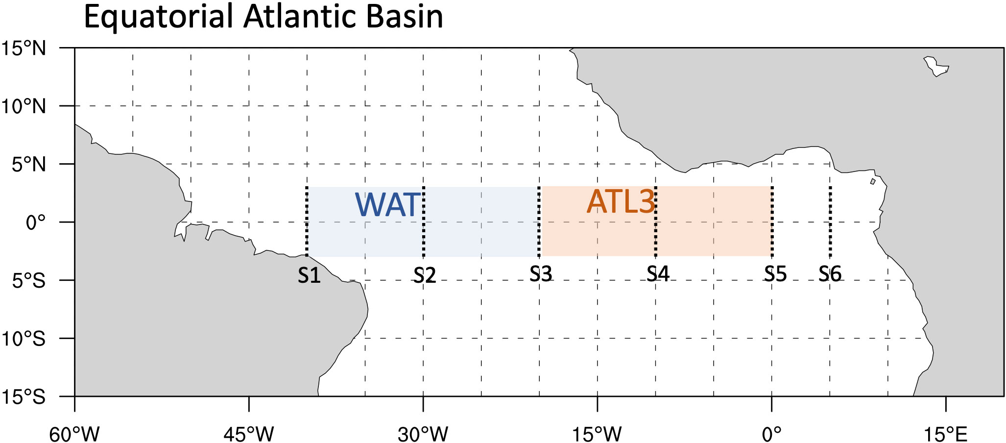
Figure 1 Tropical Atlantic Basin. The red shading covers the Atlantic 3 region (ATL3, 3°S-3°S, 20°W-0°); The blue shading covers the western equatorial Atlantic basin (WAT, 3°S-3°S, 40°W-20°W). The dotted black line indicates six meridional transections (S1-S6, at 40°W, 30°W, 20°W, 10°W, 0°, 5°E respectively) selected for the prediction model.
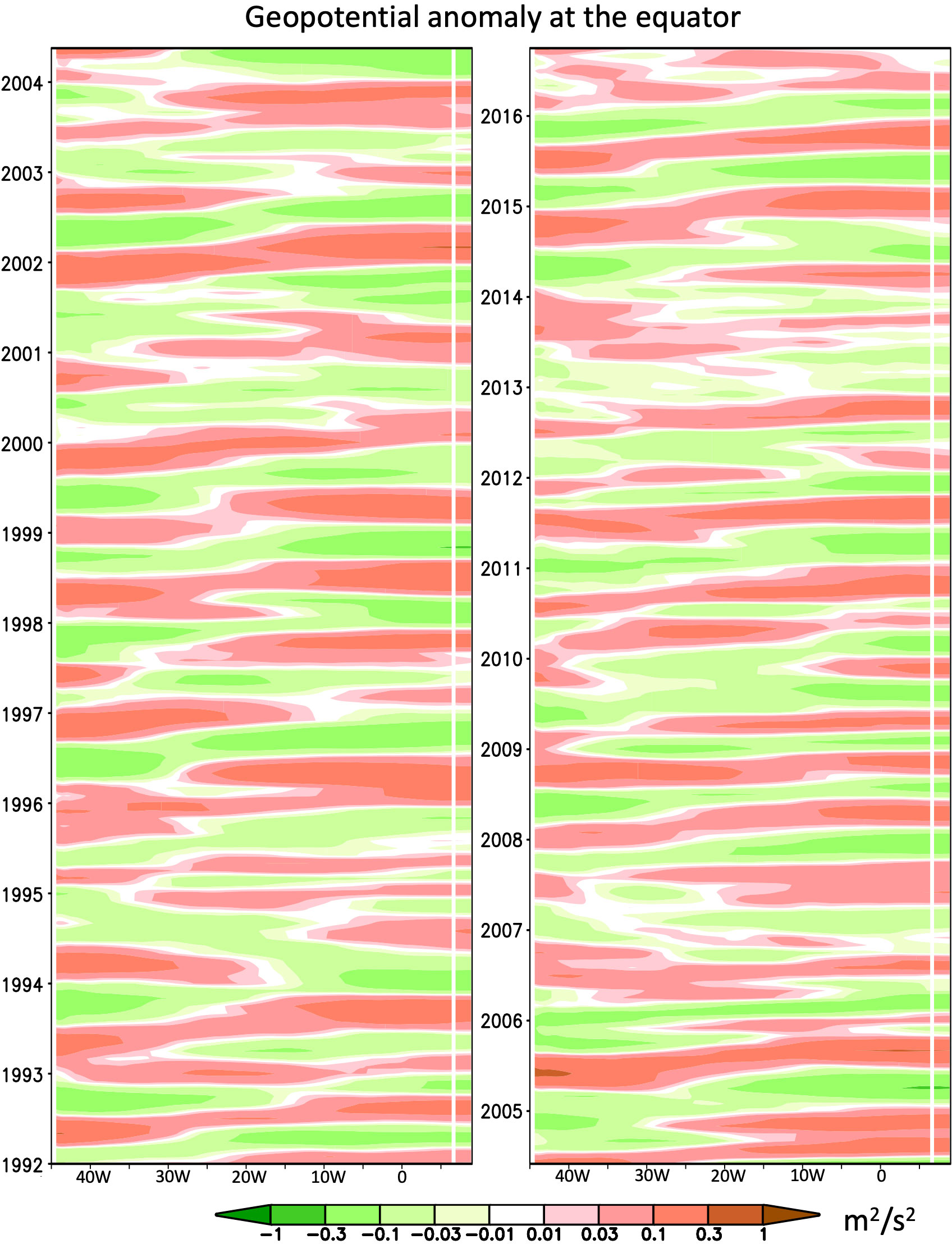
Figure 2 Hovmöller diagram for geopotential anomaly from linear ocean model at the equator in 19922004 (left panel) and 2005-2016 (right panel). Color shadings: the geopotential anomaly at the equator calculated by Equation 4.
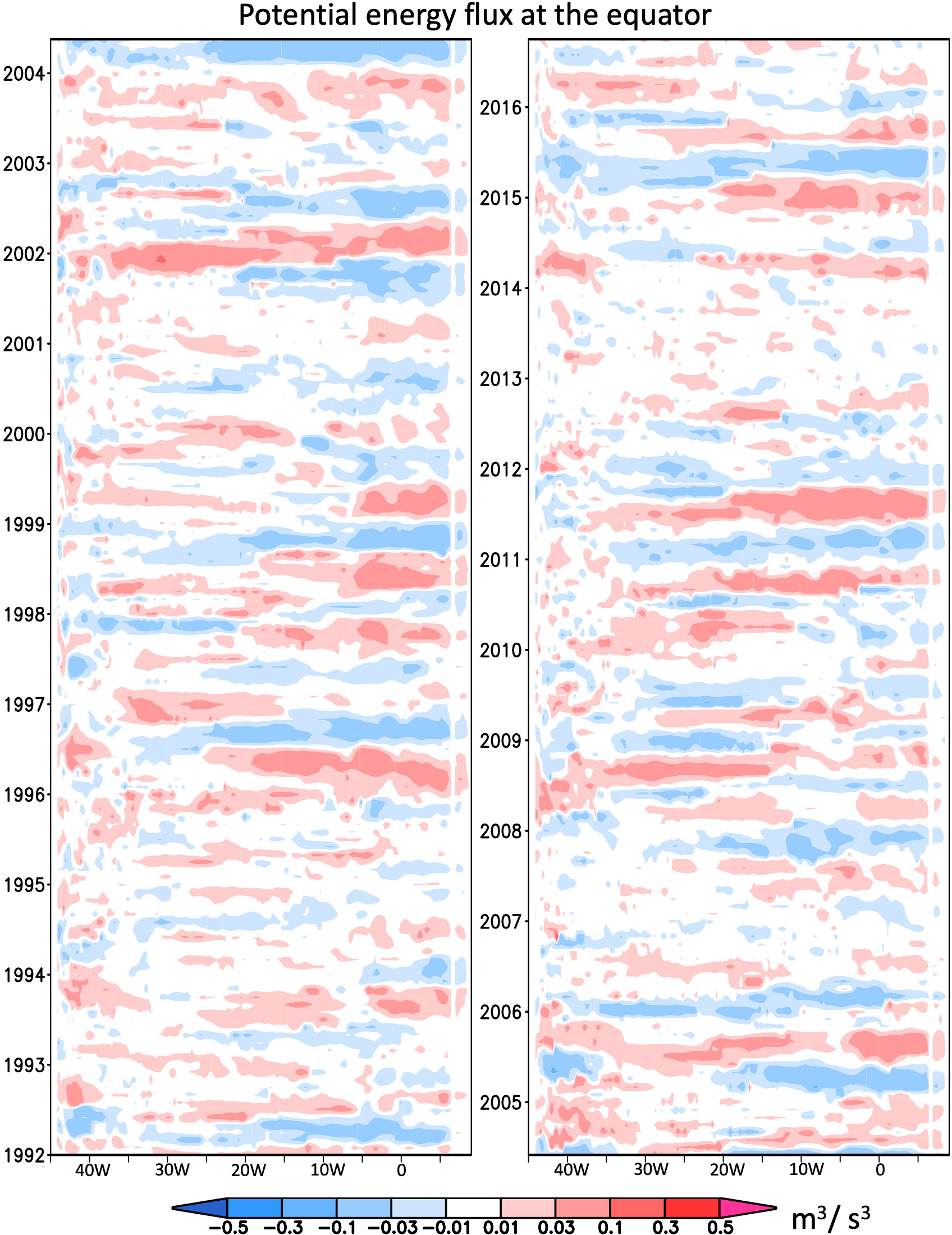
Figure 3 Hovmöller diagram for potential energy flux from linear ocean model at the equator in 1992-2004 (left panel) and 2005-2016 (right panel). Color shadings: the zonal potential energy flux at the equator following Equation 5.
We should firstly investigate the sensitivity of the prediction skill to the selected variates. Test models were built by SST and one other variate (see Figure 4A for their skills in training samples), from which the relative contribution to the prediction skill can be revealed. Figure 4B shows that the skill of the persistence is around 0.78 to predict the event leading one month, however it exhibits rapid decay with extended lead times, dropping below 0.3 after three months and plummeting to 0.12 after six months. Adding only local forcing information (shown as solid yellow line in Figure 4A) in the prediction model can barely increase the skill. By involving wave information (potential anomaly and potential energy flux) from linear ocean model, the prediction skill at a long lead month is improved. The geopotential anomaly in the ATL3 region has presented the highest improvement that increases the ACC from 0.12 to around 0.28 for six-month lead. The participation of potential flux can also contribute to improve the ACC, e.g. when the flux passing S5 (0°) is considered, the ACC increases to around 0.61 for two-month lead and 0.23 for six-month lead.
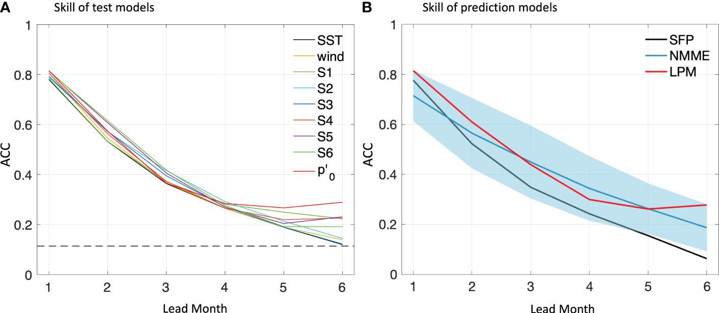
Figure 4 Anomaly correlation coefficient (ACC) of ANI in (A) test models by training samples and (B) prediction models by cross validation for the 1-6 month lead. Colored solid lines in (A) provide ACCs for test linear mode constructed by SST and one other variate as wind stress anomaly, potential flux passing S1, S2, S3, S4, S5, S6 and geopotential anomaly respectively. The solid black line in (B) is the ACC of the statistical forecast using observed SST persistence (SFP). The solid red line in (B) indicates the ACC of constructed linear prediction model (LPM). The solid blue line in (B) is the mean ACC of the selected 9 NMMEs while the blue shading covers their ACC spread. Dashed black lines indicate the ACC at the 0.05 significance level.
We can then assess the established prediction model by comparing its ACC (obtained by cross validation) with the statistical forecast using persistence and dynamical models from NMME (see Figure 4B). The NMME is an ensemble of predictions provided by a number of state-of-the-art climate models from U.S. and Canadian modelling centers. In this study, we adopted the models that cover the period from 1982 to 2018. Readers can refer to Supplementary Table 1 for the brief description of the adopted models. As Figure 4B has shown, for ANI, the prediction skill of dynamical model is generally higher than the persistence (the mean ACC is around 0.15 higher). Some dynamical models are able to provide credible SST predictions at a three-month lead (with the ACCs above 0.5), however, for the six month lead, the ACC of only one adopted NMME model is above 0.25. The established model (solid red line in Figure 4B) has revealed to have a higher ACC than the NMME mean in the prediction at the one, two and six month lead. By involving the selected variates, the skill of the prediction model at a long lead time is increased notably that the ACC exceeds 0.25 for both five-month and six-month lead, higher than most of the adopted NMME models. Also, in comparison with the statistical forecast using SST persistence, the predicted ANI (Figure 5) reduced the RMSE (root mean square error) from 0.62 to 0.57 for one-month lead, from 0.93 to 0.89 for three-month lead and from 0.97 to 0.92 for six-month lead.
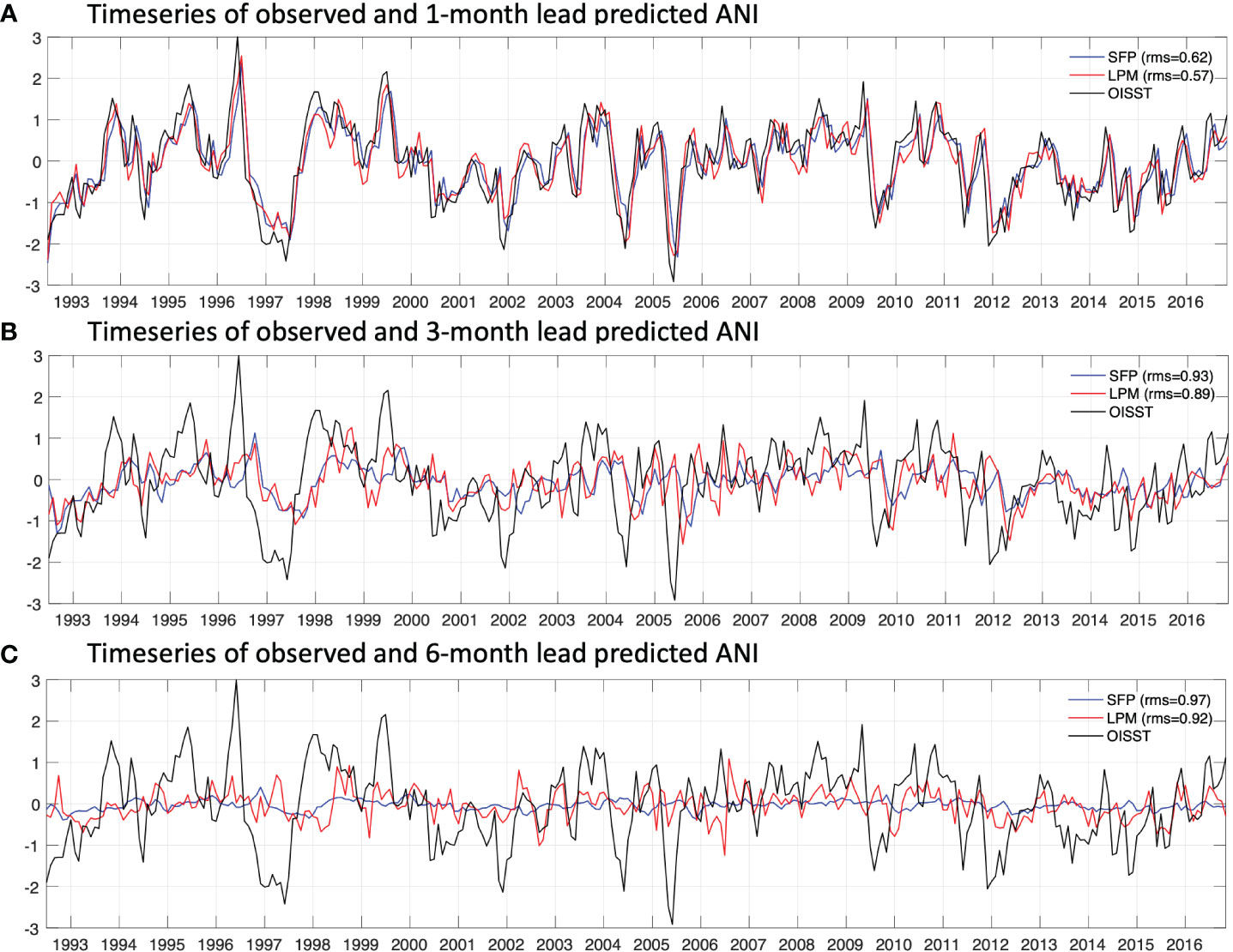
Figure 5 Timeseries of observed ANI (black solid line) and predicted ANI by statistical forecast using SST persistence (SFP, blue solid line) and linear prediction model (LPM, red solid line) from 1992 to 2016 for (A) one month lead (A), (B) three month lead and (C) six month lead.
The prediction skill is seasonally depended, namely, the ACC varies with the forecast start month (Figure 6). The ACC in Figure 6A suggests that the persistence prediction is more skilful in boreal fall and winter, while in spring and early summer (From May to July), the ACC has a dramatic drop (down to less than 0.1) for the prediction at more than two-month lead. The proposed prediction model (see Figure 6B) has a better ACC as expected, especially in the season (spring and early summer) that the SST persistence is difficult to provide a skilful prediction, e.g. in June, the ACC at the six-month lead has increased to more than 0.5. The ACC drop of the persistence prediction in boreal summer was previously reported as the predictability barrier (Dippe et al., 2019), which may due to the seasonal deepening of thermocline in the tropical Atlantic that aggrandize the role of ocean dynamics (Latif and Keenlyside, 2009). Hence by taking the geopotential and potential flux into account, we indeed involve the variates to describe dynamic evolution so as to improve the prediction skill. One other interesting point of the prediction model is that the ACC for the six-month prediction is slightly higher than the five-month or even the four-month lead prediction (see Figures 4B, 6B). This fact may imply some long-term dynamic links between the SST in ATL3 and the equatorial waves which is not locally forced (Richter et al., 2022; Song et al., 2023b).
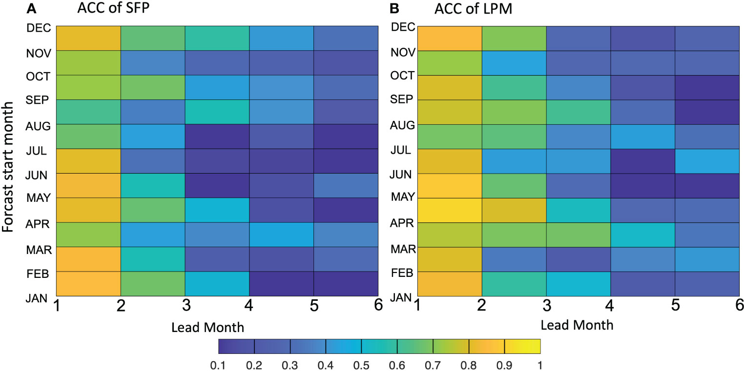
Figure 6 ACC of ANI as a function of forecast start time spanning all the calendar months (y-axis) and the lead time (x-axis) from one to six month by (A) statistical forecast using SST persistence (SFP)) and (B) linear prediction model (LPM). The ACC lower than the 0.05 significance level is blanked.
The fundamental idea of the proposed prediction model mainly relies on the process of wave propagation, however, separately analyzing equatorial waves in different baroclinic modes is difficult to provide a clear view of its combined impact on the SST anomaly in the ATL3 region (Song et al., 2023a). The lagged correlation between the superposed geopotential anomaly and ANI in Figure 7 has shown that at the one-month or two-month lead (see Figures 7A, B), the in the ATL3 region is well correlated with the SST anomaly (the correlation coefficient is above 0.4), thus adding it as one variate can slightly increase the ACC (shown as the red line in Figure 4A) of the SST persistence. The positive correlation becomes insignificant at the three-month lead and then gradually turns into negative from four-month lead to six-month lead. The temporal and spatial variation of the correlation coefficient indeed reflects how the thermocline displacement by waves are exerting their impacts on the SST event during their propagation. That is, one or two months before the SST event, the thermocline deepening in the eastern basin and the simultaneously shallowing in the western basin can make steeper the thermocline slope towards the ATL3 region hence intensifies the heat advection from the western basin and forms a dipole-like correlation pattern with ANI. At the six-month lead, the negative correlation may relate with the wave reflection. When Kelvin waves approach the eastern boundary, it will reflect as Rossby wave with opposite-sign geopotential anomaly so as to cause the SST anomaly that is negatively correlated with the original geopotential anomaly by Kelvin waves.
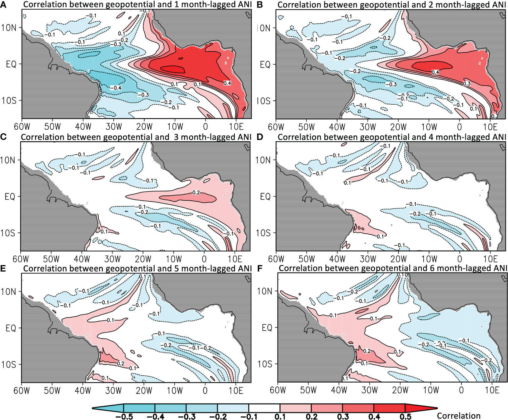
Figure 7 Correlation between the observed ANI and (A) one-month, (B) two-month, (C) three-month, (D) four-month, (E) five-month and (F) six-month lead geopotential anomaly by the linear ocean model in the tropical Atlantic. Color shading and contour are the correlation coefficient.
We then show the horizontal distribution and the variation of the potential energy flux in the tropical Atlantic basin (see Figure 8). The seasonal mean potential fluxes in both MAM (March, April and May in Figure 8A) and JJA (June, July and August in Figure 8B) are revealed to be positive in the western basin and negative in the eastern basin, converging the potential energy in the ATL3 region. As a result, the thermocline is peaked in the central basin, tilting to enhance the heat advection to the ATL3 region. In boreal fall, however, the positive potential flux extends to the whole basin changing the thermocline slope and its consequent impact on SST anomalies (see Figure 8C). Thus, the difficulty of using SST persistence to predict ANI in boreal fall (see the decrease of ACC during boreal summer in Figure 6A) might be due to the discrepancy of potential flux patterns between the two seasons and the implied seasonal change in wave dynamics.
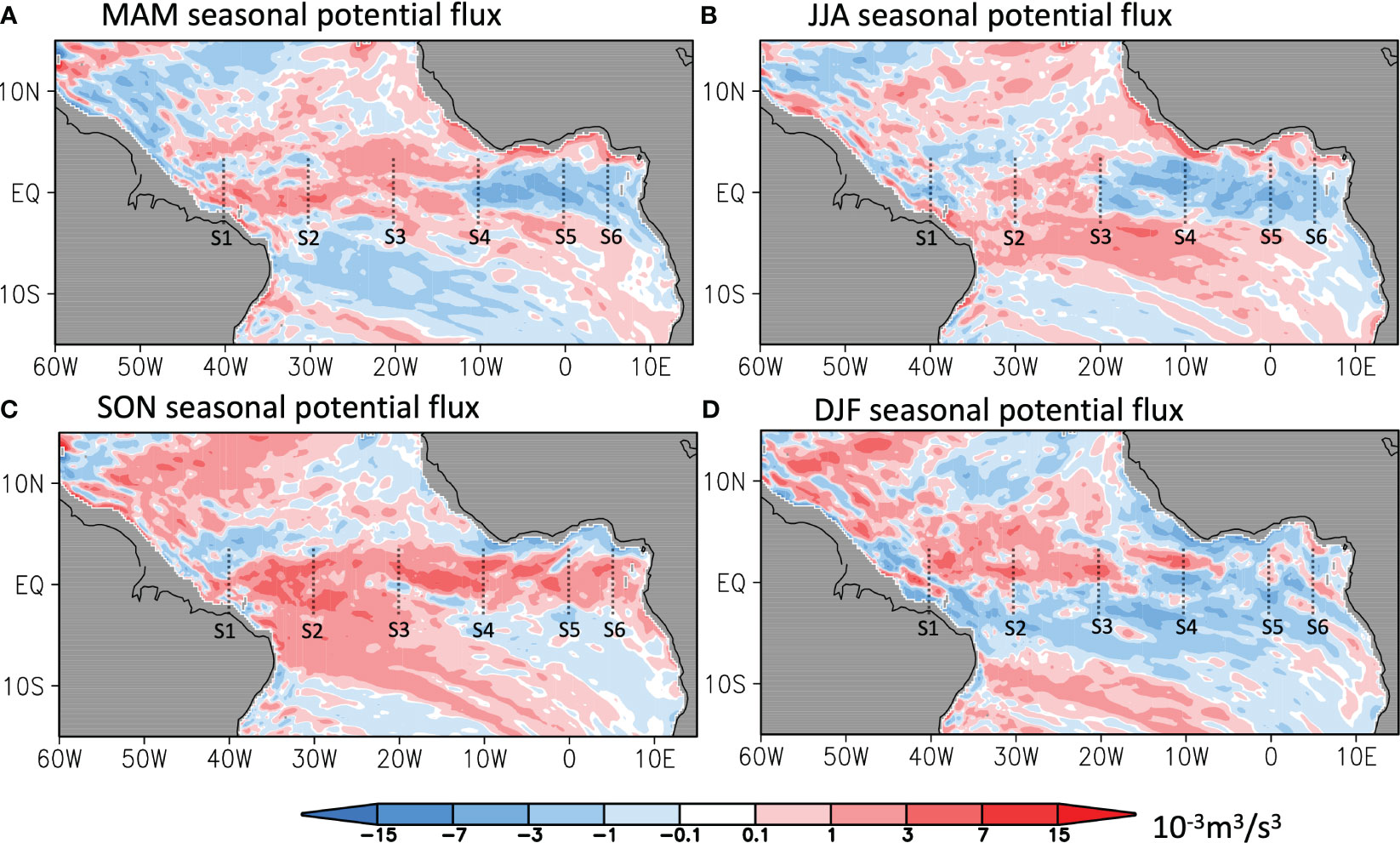
Figure 8 Seasonal zonal potential energy in the tropical Atlantic averaged in (A) MAM (March, April and May), (B) JJA (June, July and August), (C) SON (September, October and November) and (D) DFJ (December, February and January). Black dotted lines indicate the selected transections S1-S6.
The higher ACC of the prediction model at the six-month lead than the four-month or five-month lead in Figures 4B, 6B is likely associated with the remote influence through the wave propagation shown as the negative correlation in Figure 7. Nevertheless, the negative potential energy flux can be excited by either the westward wave trains with positive geopotential or the eastward wave trains with negative geopotential. Thus to identify the associated waveguide, we define the effective group velocity as follows,
where is the wave energy that the overline symbol is a phase average operator provided by Aiki et al. (2017). Following Equation 11, ce gives the averaged group velocity taking wave energy of each baroclinic mode as weights. In Figure 9, we depict the horizontal distribution of mean ce from 1992 to 2016, which reveals the eastward group velocity of around 0.3 m/s dominating the equatorial region and westward group velocity of around 0.2 m/s off the equator (Color shadings in Figure 9). Indeed, Kelvin waves propagate eastward and reflect as Rossby waves at the boundary transferring the energy back to complete the wave energy cycle (Claus et al., 2016; Song and Aiki, 2020). Thus the mean ce suggests that in the combination of westward Rossby waves and eastward Kelvin waves, the wave signal can travel through the zonal distance of around 2.5-5 degree at the equator in average by one month (see contours in Figure 9). At this group velocity, signals emerging in the ATL3 region are expected to exit the ATL3 region with Kelvin waves after four months, without returning through reflected Rossby waves. However, after six months, certain signals are anticipated to repropagate back to the ATL3 region. Hence involving the wave signal and the related dynamic process to construct the prediction model can result in the higher ACC at the six-month lead than at the four-month lead.
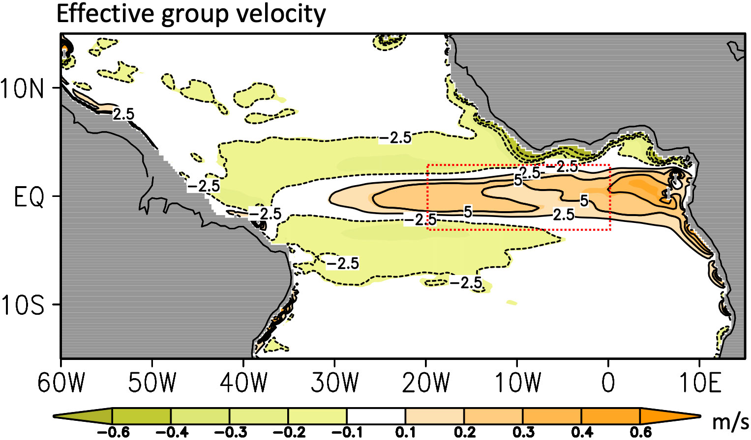
Figure 9 Mean effective zonal group velocity over 1992-2016. Color shading is the effective zonal group velocity by the three baroclinic modes following Equation 11. Contour with the interval of 2.5° present the longitude displacement at the local group velocity in one month. Red dotted box encloses the ATL3 region.
This study has constructed a linear prediction model for SST anomaly in the tropical Atlantic. By combining the observed SST, wind and the simulated signal of equatorial wave, the simple linear model provides a comparable prediction skill to the dynamical models from NMME, but the computational resource is largely reduced by applying only one-layer linear ocean model and multivariate linear regression approach. The efficacy of incorporating wave-induced geopotential anomaly and potential energy flux in enhancing predictive accuracy has been demonstrated, particularly for extended lead times. For instance, when compared to statistical forecasting based on SST persistence, the ACC for the leading six months has significantly increased, rising from 0.07 to 0.28. Notably, this improvement surpasses the performance of many dynamical models (Figure 4B). This improvement may due to a better representation of wave dynamic process in the prediction. The narrow basin scale makes Kelvin waves that induce the geopotential anomaly in ATL3, capable of passing the ATL3 region and reflecting back from the eastern boundary as Rossby waves in six months, then again displacing the thermocline in ATL3 (see Figures 7A, F). Hence the involvement of ATL3 geopotential anomaly in the model can largely increase the ACC at the six-month lead (see the test models in Figure 4A). The geopotential energy flux passing S4 and S5, additionally give the net zonal flux into the ATL3 region so as to further improve the skill. Regarding the seasonal evolution of prediction skill, the previously reported predictability barrier in dynamical models in early summer (May and June) by Dippe et al. (2019) is also found in this study. Richter et al. (2012); Voldoire et al. (2019) has suggested that the bias of atmospheric forcing (e.g. too weak trade wind) should be responsible for the drop of prediction skill in that season. Here, as Figure 8 has shown, the pressure flux pattern is changing from the Rossby-wave dominance to the Kelvin-wave dominance in the boreal summer, thus, statistical models using only initial SST and thermocline depth, e.g. the model of SST persistence and those proposed by Li et al. (2020), are difficult to predict SST anomaly at a relatively long lead time.
Certainly, this study is only one attempt to evaluate the potential of using equatorial waves to predict the Atlantic Niño/Niña events. Progresses in at least two aspects are foreseen. One is to elaborate the selection of predictor. The predictors involved in this study are all located in the latitude range, 3°S-3°N, including few off-equatorial information. However, the tropical wind anomaly could be only a part of large-scale wind pattern affected by the South Atlantic Ocean Dipole (Nnamchi et al., 2011). Also, equatorial waves have been revealed to have the second off-equatorial energy source Song et al. (2023b); Foltz and McPhaden (2010). Both facts indicate additional off-equatorial predictors. The other progress may benefit from the rapidly developed application of deep learning method in the climate predictions (Ham et al., 2019; Yu and Ma, 2021; Bi et al., 2023). The AI (artificial intelligence)-based approach e.g. the long short-term memory (LSTM) method specifically designed to handle sequential data (Zhou and Zhang, 2022), can help to find implicit dynamic associations from the selected predictors. In short, what is presented in this study is a streamlined prediction model, which utilizes the linear ocean model and wave energy flux scheme providing a comparable performance with state-of-the-art dynamical models to predict SST anomaly associated with the Atlantic zonal mode. We expect models with more intricate designs and sophisticated approaches that can further improve prediction skill in the future.
The original contributions presented in the study are included in the article/Supplementary Material, further inquiries can be directed to the corresponding author.
QS: Conceptualization, Data curation, Formal analysis, Methodology, Writing – original draft.
The author(s) declare financial support was received for the research, authorship, and/or publication of this article. The Young Scientists Fund of the National Natural Science Foundation of China (Grant Numbers 42206008) and the China Postdoctoral Science Foundation (Grant Numbers 2021M701040).
We would like to acknowledge the National Natural Science Foundation of China for the financial support. I am also grateful to the kind help from Mr. Chen Yihao for data processing.
The author declares that the research was conducted in the absence of any commercial or financial relationships that could be construed as a potential conflict of interest.
All claims expressed in this article are solely those of the authors and do not necessarily represent those of their affiliated organizations, or those of the publisher, the editors and the reviewers. Any product that may be evaluated in this article, or claim that may be made by its manufacturer, is not guaranteed or endorsed by the publisher.
The Supplementary Material for this article can be found online at: https://www.frontiersin.org/articles/10.3389/fmars.2024.1332769/full#supplementary-material
Aiki H., Greatbatch R. J., Claus M. (2017). Towards a seamlessly diagnosable expression for the energy flux associated with both equatorial and mid-latitude waves. Prog. Earth Planetary Sci. 4, 11. doi: 10.1186/s40645-017-0121-1
Bachèlery M.-L., Illig S., Rouault M. (2020). Interannual coastal trapped waves in the Angolabenguela upwelling system and benguela niño and niña events. J. Mar. Syst. 203, 103262. doi: 10.1016/j.jmarsys.2019.103262
Bi K., Xie L., Zhang H., Chen X., Gu X., Tian Q. (2023). Accurate medium-range global weather forecasting with 3D neural networks. Nature 619, 533–538. doi: 10.1038/s41586-023-06185-3
Carton J. A., Cao X., Giese B. S., Da Silva A. M. (1996). Decadal and interannual SST variability in the tropical Atlantic Ocean. J. Phys. Oceanography 26, 1165–1175. doi: 10.1175/1520-0485(1996)026<1165:DAISVI>2.0.CO;2
Chang P., Fang Y., Saravanan R., Ji L., Seidel H. (2006). The cause of the fragile relationship between the Pacific El Niño and the Atlantic Niño. Nature 443, 324–328. doi: 10.1038/nature05053
Claus M., Greatbatch R. J., Brandt P., Toole J. M. (2016). Forcing of the atlantic equatorial deep jets derived from observations. J. Phys. Oceanography 46, 3549–3562. doi: 10.1175/JPO-D-16-0140.1
Counillon F., Keenlyside N., Toniazzo T., Koseki S., Demissie T., Bethke I., et al. (2021). Relating model bias and prediction skill in the equatorial Atlantic. Climate Dynamics 56, 2617–2630. doi: 10.1007/s00382-020-05605-8
de la Vara A., Cabos W., Sein D. V., Sidorenko D., Koldunov N. V., Koseki S., et al. (2020). On the impact of atmospheric vs oceanic resolutions on the representation of the sea surface temperature in the south eastern tropical atlantic. Climate Dynamics 54, 4733–4757. doi: 10.1007/s00382-020-05256-9
Dippe T., Lübbecke J. F., Greatbatch R. J. (2019). A comparison of the Atlantic and Pacific Bjerknes feedbacks: seasonality, symmetry, and stationarity. J. Geophysical Research: Oceans 124, 2374–2403. doi: 10.1029/2018JC014700
Foltz G. R., Brandt P., Richter I., Rodríguez-Fonseca B., Hernandez F., Dengler M., et al. (2019). The tropical Atlantic observing system. Front. Mar. Sci. 6, 206. doi: 10.3389/fmars.2019.00206
Foltz G. R., McPhaden M. J. (2010). Interaction between the Atlantic meridional and Niño modes. Geophysical Res. Lett. 37. doi: 10.1029/2010GL044001
Giannini A., Saravanan R., Chang P. (2003). Oceanic forcing of sahel rainfall on interannual to interdecadal time scales. Science 302, 1027–1030. doi: 10.1126/science.1089357
Ham Y.-G., Kim J.-H., Luo J.-J. (2019). Deep learning for multi-year ENSO forecasts. Nature 573, 568–572. doi: 10.1038/s41586-019-1559-7
Illig S., Bachèlery M.-L. (2019). Propagation of subseasonal equatorially-forced coastal trapped waves down to the benguela upwelling system. Sci. Rep. 9, 1–10. doi: 10.1038/s41598-019-41847-1
Imbol Koungue R. A., Illig S., Rouault M. (2017). Role of interannual k elvin wave propagations in the equatorial a tlantic on the a ngola b enguela c urrent system. J. Geophysical Research: Oceans 122, 4685–4703. doi: 10.1002/2016JC012463
Imbol Koungue R. A., Rouault M., Illig S., Brandt P., Jouanno J. (2019). Benguela niños and benguela niñas in forced ocean simulation from 1958 to 2015. J. Geophysical Research: Oceans 124, 5923–5951. doi: 10.1029/2019JC015013
Keenlyside N. S., Ding H., Latif M. (2013). Potential of equatorial Atlantic variability to enhance El Niño prediction. Geophysical Res. Lett. 40, 2278–2283. doi: 10.1002/grl.50362
Koungue I., Rodrigue A., Brandt P., Lübbecke J., Prigent A., Martins M., et al. (2021). The 2019 benguela niño. Front. Mar. Sci. 8. doi: 10.3389/fmars.2021.800103
Latif M., Keenlyside N. S. (2009). El Niño/Southern Oscillation response to global warming. Proc. Natl. Acad. Sci. 106, 20578–20583. doi: 10.1073/pnas.0710860105
Li X., Bordbar M. H., Latif M., Park W., Harlaß J. (2020). Monthly to seasonal prediction of tropical Atlantic sea surface temperature with statistical models constructed from observations and data from the Kiel Climate Model. Climate Dynamics 54, 1829–1850. doi: 10.1007/s00382-020-05140-6
Lübbecke J. F., McPhaden M. J. (2012). On the inconsistent relationship between Pacific and Atlantic Niños. J. Climate 25, 4294–4303. doi: 10.1175/JCLI-D-11-00553.1
Nnamchi H. C., Li J., Anyadike R. N. (2011). Does a dipole mode really exist in the South Atlantic Ocean? J. Geophysical Research: Atmospheres 116. doi: 10.1029/2010JD015579
Okumura Y., Xie S.-P. (2004). Interaction of the Atlantic equatorial cold tongue and the African monsoon. J. Climate 17, 3589–3602. doi: 10.1175/1520-0442(2004)017<3589:IOTAEC>2.0.CO;2
Richter I., Behera S. K., Masumoto Y., Taguchi B., Sasaki H., Yamagata T. (2013). Multiple causes of interannual sea surface temperature variability in the equatorial Atlantic Ocean. Nat. Geosci. 6, 43–47. doi: 10.1038/ngeo1660
Richter I., Tokinaga H., Okumura Y. M. (2022). The extraordinary equatorial Atlantic warming in late 2019. Geophysical Res. Lett. 49, e2021GL095918. doi: 10.1029/2021GL095918
Richter I., Xie S.-P., Wittenberg A. T., Masumoto Y. (2012). Tropical atlantic biases and their relation to surface wind stress and terrestrial precipitation. Climate dynamics 38, 985–1001. doi: 10.1007/s00382-011-1038-9
Rodríguez-Fonseca B., Polo I., García-Serrano J., Losada T., Mohino E., Mechoso C. R., et al. (2009). Are Atlantic Niños enhancing pacific enso events in recent decades? Geophysical Res. Lett. 36. doi: 10.1029/2009GL040048
Schiller A., Wijffels S., Sprintall J., Molcard R., Oke P. R. (2010). Pathways of intraseasonal variability in the Indonesian throughflow region. Dynamics atmospheres oceans 50, 174–200. doi: 10.1016/j.dynatmoce.2010.02.003
Servain J., Wainer I., McCreary J. P. Jr., Dessier A. (1999). Relationship between the equatorial and meridional modes of climatic variability in the tropical Atlantic. Geophysical Res. Lett. 26, 485–488. doi: 10.1029/1999GL900014
Smagorinsky J. (1963). General circulation experiments with the primitive equations: I. @ the basic experiment. Monthly Weather Rev. 91, 99–164. doi: 10.1175/1520-0493(1963)091<0099:GCEWTP>2.3.CO;2
Small R. J., Curchitser E., Hedstrom K., Kauffman B., Large W. G. (2015). The benguela upwelling system: Quantifying the sensitivity to resolution and coastal wind representation in a global climate model. J. Climate 28, 9409–9432. doi: 10.1175/JCLI-D-15-0192.1
Song Q., Aiki H. (2020). The climatological horizontal pattern of energy flux in the tropical atlantic as identified by a unified diagnosis for rossby and kelvin waves. J. Geophysical Research: Oceans 125, e2019JC015407. doi: 10.1029/2019JC015407
Song Q., Aiki H. (2021). Horizontal energy flux of wind-driven intraseasonal waves in the tropical Atlantic by a unified diagnosis. J. Phys. Oceanography 51, 3037–3050. doi: 10.1175/JPO-D-20-0262.1
Song Q., Aiki H. (2023). Equatorial wave diagnosis for the atlantic niño in 2019 with an ocean reanalysis. Ocean Sci. 19, 1705–1717. doi: 10.5194/os-19-1705-2023
Song Q., Aiki H., Tang Y. (2023a). The role of equatorially forced waves in triggering Benguela Niño/Niña as investigated by an energy flux diagnosis. J. Geophysical Research: Oceans, 128 (4),e2022JC019272. doi: 10.1029/2022JC019272
Song Q., Tang Y., Aiki H. (2023b). Dual wave energy sources for the atlantic niño events identified by wave energy flux in case studies. J. Geophysical Research: Oceans 128, e2023JC019972. doi: 10.1029/2023JC019972
Stockdale T. N., Balmaseda M. A., Vidard A. (2006). Tropical Atlantic SST prediction with coupled ocean–atmosphere GCMs. J. Climate 19, 6047–6061. doi: 10.1175/JCLI3947.1
Voldoire A., Exarchou E., Sanchez-Gomez E., Demissie T., Deppenmeier A.-L., Frauen C., et al. (2019). Role of wind stress in driving SST biases in the Tropical Atlantic. Climate Dynamics 53, 3481–3504. doi: 10.1007/s00382-019-04717-0
Wang R., Chen L., Li T., Luo J.-J. (2021). Atlantic niño/niña prediction skills in NMME models. Atmosphere 12, 803. doi: 10.3390/atmos12070803
Yu S., Ma J. (2021). Deep learning for geophysics: Current and future trends. Rev. Geophysics 59, e2021RG000742. doi: 10.1029/2021RG000742
Zhou L., Zhang R.-H. (2022). A hybrid neural network model for enso prediction in combination with principal oscillation pattern analyses. Adv. Atmospheric Sci. 39, 889–902. doi: 10.1007/s00376-021-1368-4
This section provides a simple introduction for the linear ocean model to provide the wave signal, which readers can refer to Song and Aiki (2020, 2021) for more detailed information. The governing equations of the linear ocean model to simulate equatorial waves are as follows,
where p(n) is the geopotential, (u(n),v(n)) are the horizontal components of velocity and the subscript n stands for the n-th baroclinic mode. D represents the horizontal eddy viscosity estimated by Smagorinsky (1963) c(n) is the phase speed of non-rotating gravity waves and H(n) represents the wind forcing portion to drive the n-th baroclinic mode, which are both solved from eigen equation in the vertical direction as follows,
By estimating the Brunt-Väisölä frequency N from the climatological annual mean vertical profiles of temperature and salinity data in the World Ocean Atlas (WOA), c(n) and the corresponding eigenfunction Ψ(n) are obtained. Then H(n) reads,
Where hmix is the mixed layer depth and Hb is the water depth respectively. hmix (48m) and Hb (4500m) are both constant in this study. Readers can check Table 1 and Figure 1 in Song et al. (2023a) for the applied c(n), H(n) and Ψ(n) in the first three baroclinic modes by Equation (A.3). For the concerned tropical Atlantic Ocean, the model can be regarded as having radiation boundaries in the north and south where no wave reflections are expected.
An energy budget equation for shallow water waves in the presence of wind forcing and eddy viscosity reads,
where is wave energy of the nth mode (including both kinetic and potential energies), and stands for the velocity and viscosity force vector respectively. is the wind forcing power, and is the eddy viscosity stress power. The overline symbol in Equation (A.4) is a phase average operator provided by Aiki et al. (2017). By adding a rotational term to the geopotential flux , the AGC-L2 scheme is able to provide an expression of the group-velocity-based energy flux for equatorial waves at all latitudes to read,
which includes a scalar quantity φ. This quantity is defined as
where is the Ertel’s potential vorticity. The rotational flux in Equation (A.5) can redirect the vector to head in the direction of group velocity for different-type-of waves in tropical basins (Aiki et al., 2017). Equation (A.6) is a diagnostic equation by which (φ(n))app can be obtained directly from the EPV q(n). We can hence define the effective group velocity as
Keywords: equatorial wave, Atlantic Niño, prediction model, wave energy flux, sea surface temperature
Citation: Song Q (2024) An attempt using equatorial waves to predict tropical sea surface temperature anomalies associated with the Atlantic zonal mode. Front. Mar. Sci. 11:1332769. doi: 10.3389/fmars.2024.1332769
Received: 03 November 2023; Accepted: 19 January 2024;
Published: 22 February 2024.
Edited by:
Kyung-Ae Park, Seoul National University, Republic of KoreaReviewed by:
Chunxue Yang, National Research Council (CNR), ItalyCopyright © 2024 Song. This is an open-access article distributed under the terms of the Creative Commons Attribution License (CC BY). The use, distribution or reproduction in other forums is permitted, provided the original author(s) and the copyright owner(s) are credited and that the original publication in this journal is cited, in accordance with accepted academic practice. No use, distribution or reproduction is permitted which does not comply with these terms.
*Correspondence: Qingyang Song, cXlzb25nQGhodS5lZHUuY24=
Disclaimer: All claims expressed in this article are solely those of the authors and do not necessarily represent those of their affiliated organizations, or those of the publisher, the editors and the reviewers. Any product that may be evaluated in this article or claim that may be made by its manufacturer is not guaranteed or endorsed by the publisher.
Research integrity at Frontiers
Learn more about the work of our research integrity team to safeguard the quality of each article we publish.