 Jack Sheehy
 Richard Bates2
 Michael Bell
 Jo Porter
- 1International Centre for Island Technology, Heriot-Watt University, Stromness, United Kingdom
- 2School of Earth and Environmental Sciences, University of St Andrews, St Andrews, United Kingdom
Horse mussel beds are listed as a Priority Marine Feature (PMF) in Scotland for their influence in the creation of diverse benthic communities and provision of ecosystem services. In Scotland, horse mussel beds are also recognised for their importance in marine carbon sequestration. Unfortunately, there is a paucity of data on horse mussel bed carbon stocks and sediment thickness. There are also significant financial and logistical barriers with which to address these data gaps. This study investigates the robustness of Sub-Bottom Profiling (SBP) as a cost-effective method to quantify horse mussel sediment thickness across a landscape. Integrating SBP and Drop-Down Video (DDV) data, this study also details an integrated approach to investigate the links between horse mussel habitat condition and sediment thickness. With the addition of abiotic data, this study uses Structural Equation Modelling (SEM) to elucidate key relationships between abiotic factors, biotic variables, and sediment thickness. There is a significant positive correlation of horse mussel habitat condition and sediment thickness. Average horse mussel total sediment thickness, across all measures of habitat condition, was 1.37m. These findings substantially increase previous estimates of horse mussel sediment thickness, and potential value to climate change mitigation through blue carbon frameworks. This study highlights the importance of both abiotic and biotic factors on marine carbon sediment quantification.
Introduction
The horse mussel, Modiolus modiolus, form beds on the benthic substrate, creating suitable habitat for a plethora of species (Fariñas-Franco et al., 2023). Due to their importance for local biodiversity and ecosystem function, in Scotland they are detailed as a Priority Marine Feature (Tyler-Walters et al., 2016). Additionally, due to their sensitivity to a range of threats, they are also listed as a UK Biodiversity Action Plan (BAP) habitat (JNCC, 2019), afforded protection under the Habitats Directive (Jones et al., 2000), and are listed as a threatened and declining habitat through the Oslo and Paris (OSPAR) Convention (Ospar Commission, 2021).
Horse mussel beds have the potential to sequester both organic carbon (OC) and inorganic carbon (IC) in living matter as well as in underlying sediments. In Scotland, as a ‘biogenic reef’ they are considered a ‘blue carbon’ species (Shafiee, 2018; Porter et al., 2020). They are not, however, defined as a ‘blue carbon’ species in international frameworks (IPCC, 2014) due to data gaps and uncertainty of carbon stocks and carbon sequestration potential. Research that therefore clarifies this uncertainty may support their integration into policy and ecological conservation through an eco-social economics approach (Lovelock and Duarte, 2019; Sheehy et al., 2022, 2024a).
As abiotic hydrodynamic factors largely determine sediment deposition across a benthic landscape, potential blue carbon habitats must likewise prove an additional benefit to carbon sequestration beyond that of abiotic hydrodynamics and/or other factors (Röhr et al., 2018). Identifying the relative importance of abiotic and biotic factors, and their interactive effects, on blue carbon habitats are essential to medium to large scale quantification and management of carbon stocks (Malerba et al., 2023; Sheehy et al., 20231). Small, medium, and large scale are defined as 0.05-0.1 km2, 1 km2, and >1,000 km2 respectively (Malerba et al., 2023). Blue carbon research has predominantly focused on extrapolation of single point core data across habitats (Macreadie et al., 2014) but extrapolation of these data across a habitat has inherent uncertainty (Howard et al., 2014).
Horse mussel bed morphology is largely dictated by local hydrodynamics and environmental conditions. Horse mussel beds may be found directly attached to hard substrata (Holt et al., 1998), or partially embedded into sediment with juveniles linked through the byssal threads of adults (Tyler-Walters, 2007). Horse mussel beds trap faecal mud, sediment, and shell debris which act to increase the depth of the horse mussel bed along with new growth on top of old matter; strong currents may therefore determine the retention and sedimentation of matter and prevent the formation of raised horse mussel beds (Holt et al., 1998). On coarse sediment, horse mussels may also bind the sediment together creating nests of infaunal mounds in wave form; these can grow up to 3m high, 20m wide, and 10-100m in length (Wildish and Fader, 1998). Around the British isles, mounds up to 1m have been reported in the Isle of Man and in Ireland (Holt et al., 1998; Lindenbaum et al., 2008).
Interactive effects of abiotic and biotic factors will also determine the composition of horse mussel bed associated communities (Holt et al., 1998). Horse mussel beds create complex habitats that significantly affect benthic composition (Ragnarsson and Burgos, 2012). Healthy horse mussel beds support high biodiversity (Sanderson et al., 2014; Mackenzie et al., 2018), carbon sequestration processes (Burrows et al., 2017; Porter et al., 2020), water quality (Navarro and Thompson, 1996), and species important to fisheries (Rees, 2009; Kent et al., 2017). Horse mussels can be found individually, or in densities up to 600 individuals m2 (Lindenbaum et al., 2008). In dense reefs, the complexity of the habitat adds to habitat condition and biodiversity where species benefit from increased benthic production, structural variation, and ecological niches (Rees, 2009; Marine Scotland, 2018).
The sedimentary composition of horse mussel beds are principally determined by the habitat condition, and the composition of the associated faunal communities (Holt et al., 1998; Fariñas-Franco et al., 2014; Saderne et al., 2019); these determine carbon fluxes and the ratios of allochthonous input and autochthonous export. Horse mussels have been found to account for 93.5% of Inorganic Carbon (IC) in horse mussel bed communities, but account for only 37.8% of estimated production; the remaining production derived from associated horse mussel bed fauna and flora (Collins, 1986). The potential of a shellfish reef, or horse mussel bed, to act as a carbon sink, is therefore dependent upon the ‘relative balance between organic and inorganic carbon burial’ (Fodrie et al., 2017). Both carbon stocks in horse mussel shells and in sediment can be considered sequestered (Collins, 1986; Burrows et al., 2014, 2017; Porter et al., 2020; Sheehy et al., 2024a). ‘Mussel mud’ locked in the horse mussel bed may store carbon on even longer timescales (Mainwaring et al., 2014; Armstrong et al., 2020). There is, however, a paucity of data on the carbon sequestration potential of horse mussel habitats. In the UK, horse mussel sediment carbon content is generally extrapolated from one grab sample that reached a maximum sediment depth of 5-7cm (Collins, 1986). Yet due to differences in sediment diagenesis across depth (Fourqurean and Schrlau, 2003), and carbon sequestration over time (Kennedy et al., 2010; Pedersen et al., 2011), blue carbon sediment composition varies with sediment depth (MacLeod, 20152; Potouroglou et al., 2021).
Mean horse mussel carbon content density, 2,219 g CaCO3 m-2 (Collins, 1986; Burrows et al., 2014), is generally extrapolated to a mean thickness of 0.75m (Burrows et al., 2017; Porter et al., 2020), from one study detailing acoustically observed horse mussel wave forms ranging in sediment thickness from 0.5m to 1m (Lindenbaum et al., 2008). Whilst there are data on the links between habitat condition and blue carbon sediment stocks (Ricart et al., 2017; Röhr et al., 2018; Sheehy et al., 20231; Sheehy et al., 2024b), there are no specific data of this type for horse mussel beds.
This study investigates the feasibility of Sub-Bottom Profiling (SBP) in determining horse mussel sediment thickness. This study subsequently furthers limited research of acoustic sounding techniques in blue carbon science (Lo Iocano et al., 2008; Tomasello et al., 2009; Hunt et al., 2020, 2021; Monnier et al., 2021). Specific to horse mussel habitats, it provides data on horse mussel sediment thickness to update previous UK estimates using acoustic data (Lindenbaum et al., 2008). Linking SBP data to Drop-Down Video (DDV) data to quantify habitat condition as horse mussel percentage cover provides a way to identify correlations of horse mussel bed abundance with sediment thickness. This integrated approach supports cost-effective, easily applicable, small to medium scale quantification of blue carbon resources and by extension community level societal engagement to protect marine habitats (Sheehy et al., 2024a). When considered with future research techniques and needs, including machine learning approaches and regional assessments of blue carbon stocks, SBP and DDV data may be ‘stacked’ with predictive modelling outputs to better identify key areas for marine conservation (Pinto-Ledezma and Cavender-Bares, 2021; Malerba et al., 2023; Sheehy et al., 20231; Sheehy et al., 2024a, 2024b).
Horse mussel habitat is prevalent in the Atlantic on European and North American coastlines, but can also be found in the Pacific in addition to the Indian Ocean (Ocean Biodiversity Information System [OBIS], 2022). They are suited to a range of tidal current strengths and exposure except strong wave exposure (Tyler-Walters, 2007). They can be found on both soft and hard substrates. Horse mussels are generally tolerant of a range of depths (Wildish and Fader, 1998), but favour depths of 5m to 50m in the UK (Holt et al., 1998). Matching these environmental conditions, extensive horse mussel beds are most commonly found on the north and western coasts of the UK (Tyler-Walters, 2007). In Orkney, there is an estimated 38.28 km2 of horse mussel beds but this is, however, a potential estimate of total extent of multiple horse mussel habitats across the area, rather than a single horse mussel bed, and is subject to large uncertainty (Porter et al., 2020). Limited data also constrains estimates of horse mussel carbon content in underlying sediment to be generally constrained to a thickness of 0.75m (Porter et al., 2020).
The overall aim of this study is to determine the feasibility and robustness of SBP data in characterising horse mussel bed sediment thickness and to investigate the interactions of abiotic and biotic factors on horse mussel sediment thickness. The objectives of this paper are:
• To present the feasibility of SBP data to detail horse mussel bed sediment thickness.
• To demonstrate the use of SBP data for mapping horse mussel bed sediment thickness.
• To determine the relative influences and interactions of environmental variables and horse mussel bed habitat condition (based on horse mussel percentage cover) on horse mussel bed sediment thickness.
• To highlight key areas of future research for quantification of horse mussel bed sediments within the context of blue carbon science and accreditation processes.
Methods
Study sites
The survey area was limited to Orkney, Scotland. A key site was identified off the eastern coast of the mainland of Orkney, south of the island of Shapinsay and east of the island of Helliar Holm. The survey area is defined in Figure 1.
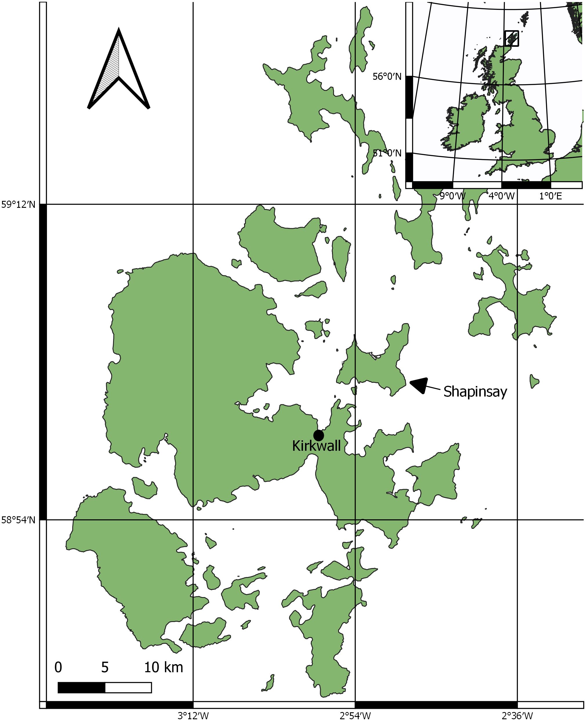
Figure 1 Regional survey area for horse mussel data collection.
Suitable locations to survey horse mussel habitats, at likely horse mussel habitat locations, were identified from contemporary literature where Maximum Entropy (MAXENT) predicted models were used to predict horse mussel habitats (Porter et al., 2020), online records of horse mussel habitats (NBN, 2017), and from local fishers expertise and knowledge. A key location was identified south of Shapinsay (59°01’37.2”N 2°55’25.3”W). The area features a mosaic of horse mussel abundance on a slope of gravel and dead shell substrate. The slope ranges in depth from ~12m to ~23m. The tidal range for Kirkwall, the nearest port, is 3.2m; Kirkwall has a maximum tidal height of 3.4m and minimum of -0.2m (TideTimes, 2023).
Survey design and protocol
This study collates regional abiotic current and wave exposure data (Burrows, 2007; Almoghayer et al., 2022) with core data from local mud, seagrass, and maerl habitats (Bates et al., 2014; MacLeod, 20152) to support the research aims; core data were used to support feasibility assessment and demonstration of Sub-Bottom Profiling (SBP) data for horse mussel bed thickness estimation whilst abiotic data were used to support analysis of the variables influences on horse mussel bed thickness. The survey collected SBP data with which to detail seabed depth (at fine scale) and horse mussel bed sediment thickness. DDV data was collected to map horse mussel bed percentage cover. Survey data collection was conducted onboard MV Challenger with the help of a local marine operations consultancy team with previous experience in SBP data collection (SULA, 2018).
Prior to SBP data surveying, survey sites were first checked for horse mussel presence with DDV. DDV footage was recorded, with Global Positioning Systems (GPS) data used from the boat track plotter to align DDV footage with location. To avoid later propellor distortion on SBP data, the survey vessel was allowed to drift with local currents at speeds below 4 kn; survey transect lines were set in conjunction with tide times to ensure replicable boat drift. DDV footage was first assessed in real time to identify and locate horse mussel bed presence and suitable transect lines. DDV footage was then reviewed again in desktop review to assess and record spatial distribution of horse mussel abundance. Abundance as percentage cover was recorded at discrete points along transect survey lines. Five suitable survey transect lines were identified, based on horse mussel presence and abundance and in conjunction with tide times, to support subsequent SBP data collection for the Shapinsay horse mussel (SHH) survey site. The five survey transect lines are hereafter referred to as SHH1, SHH2, SHH3, SHH4 and SHH5.
SBP surveys were then conducted on the same transect lines used for the DDV data collection, using the same method of current drift with the DDV, and with GPS positioning data recorded from the SBP. Data were recorded with an Innomar Compact SES 2000, fixed to the side of the boat using a bespoke attachment pole, specially constructed to fit MV Challenger, for SBP surveys. Due to the novel nature of this approach for blue carbon sediment thickness estimation, multiple operating frequencies were used. Transect lines were surveyed twice, simultaneously at Low Frequency (LF) at 8kHz at -6dB and High Frequency (HF) at 10kHz and 7dB, and then again using the multi-frequency (MF) setting which simultaneously recorded data LF data (at -6dB) and HF data (at 7dB) at 5kHz, 10kHz, and 15kHz. All data were recorded in RAW file format to capture all potential survey data. All SBP data channels and settings are detailed in the Supplementary Material.
Survey data were named per transect line, with a first number for the general transect line, and a second number to denote the SBP setting for that specific transect line run. For example, SHH11 was conducted on transect line 1 with the MF setting, and SHH12 was conducted on transect line 1 with the LF/HF setting. All SBP transects are listed as SHH11, SHH12, SHH21, SHH22, SHH31, SHH32, SHH41, SHH42, SHH51, and SHH52. Survey transects and survey areas are detailed in Figures 2 and 3.
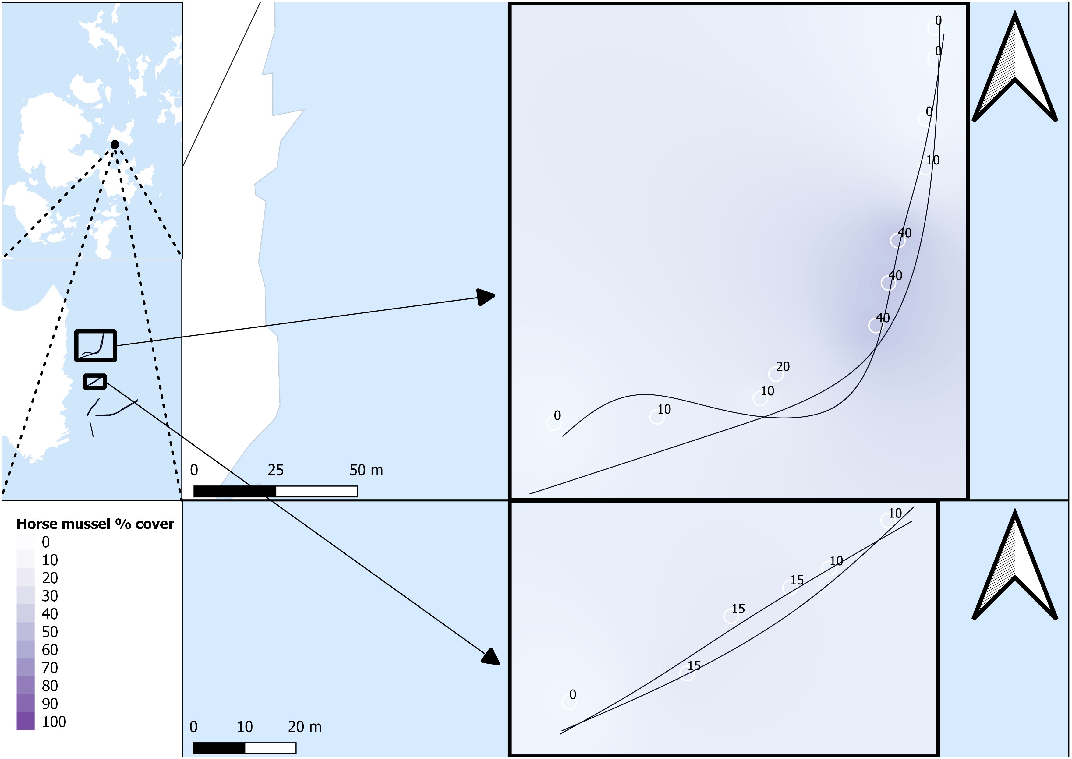
Figure 2 Horse mussel transects. SHH11 and SHH12 (top) and SHH21 and SHH22 (bottom). Horse mussel percentage cover data from DDV is detailed along the transect paths.
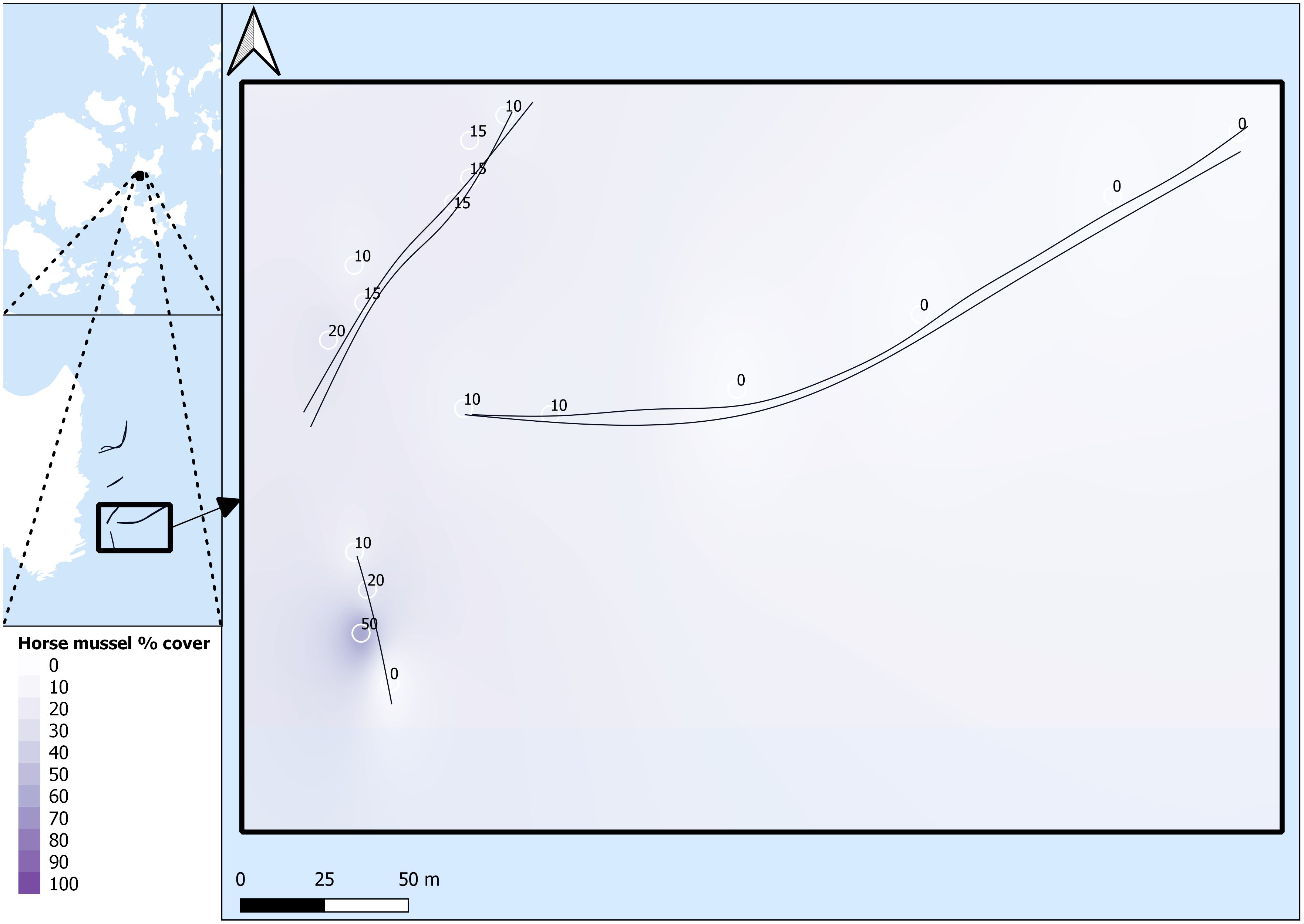
Figure 3 Horse mussel transects. SHH31 and SHH32 (top left), SHH41 and SHH42 (right), and SHH51 and SHH52 (bottom left). Horse mussel percentage cover data from DDV is detailed along the transect paths.
Data alignment with percentage cover
SBP data were converted to SEG-Y file format using Innomar SES Convert software (Innomar, 2023). SEG-Y data.txt files were also created to allow for import of ping data with GPS position into QGIS (QGIS, 2023). Horse mussel abundance, estimated visually as percentage cover from DDV data, was also imported into QGIS with waypoint GPS data. Abundance as percentage cover was interpolated using the Inverse Distance Weighted (IDW) method, to convert point data to a contiguous map over the transect line, then added to abiotic and SBP ping data. Data points with no horse mussel percentage cover were removed to avoid potential bias of data from inclusion of non-horse mussel habitats, and to maintain the focus of this study on the effects of horse mussel habitat on sediment thickness rather than other substrate sediment thickness. Data were exported to txt. file format and imported into SeiSee software (SeiSee, 2023) to then add horse mussel bed percentage cover to SEG-Y data files. Subsequently, these SEG-Y files were imported into Sonarwiz seafloor mapping and analysis software (Chesapeake Technology, 2023).
Alignment with core data
There are no core records detailing horse mussel bed sediment composition. However, SBP data were aligned to general patterns of strata with differing Organic Carbon (OC)/Inorganic Carbon (IC) content observed in local cores from analogous research for seagrass (Sheehy et al., 2023b1) and maerl (Sheehy et al., 2024b); whilst core data were not available for horse mussel beds or for the horse mussel habitat survey transects, clear patterns of strata and OC/IC content were identified and observable in core data for mud substrate, and seagrass, and maerl bed sediments. Core data strata patterns (sediment layers) were observable in SBP data for mud substrate, seagrass, maerl, and horse mussel bed sediments. It was therefore felt that SBP data were analogous between these different habitats and allowed a relative confidence with which to identify likely sediment layers and strata composition in horse mussel bed sediments. Accordingly, the same channels and settings used to identify sediment layers in analogous research for seagrass and maerl habitats (Sheehy et al., 20231; Sheehy et al., 2024b), were also used to identify horse mussel bed sediment layers. Layers were identified with varying resolution and definition dependent on the SBP setting, with different results observed due to differences in channel dB and kHz ranges. The HF1 channel data were identified as the most suitable for shallow predominantly organic layers of sediment, hereafter referred to as the Shallow Sediment Thickness (SST). The total horse mussel bed sediment thickness, hereafter referred to as the Total Sediment Thickness (TST) was taken from the LF3 channel data.
The horse mussel bed had the greatest percentage cover on a benthic slope, and horse mussel bed percentage cover ranged from 10% to 40% cover. Key features, including underlying bedrock features, patterns in the strata (sediment layers), and sediment thickness variability with horse mussel percentage cover, were observed in the SBP data. Identification of these key features, which also matched analysis from analogous research (Sheehy et al., 20231; Sheehy et al., 2024b), was taken as confirmation of correct identification of sediment layers and correlation with SBP data rather than erroneous identification of sediment from acoustic background noise or interference.
HF1 data alignment of percentage cover, depth, seabed, and bedrock identification are shown in Figure 4. The data show the benthic depth increasing from left to right along a slope, with depth markers at every 2m and aligned vertically with horse mussel bed percentage cover values. From the seabed there is first an immediate thin light grey layer believed to be surface organic biomass; whilst this is not ground-truthed (there are no core data for horse mussel beds) this was observed and ground truthed for seagrass and maerl habitats (Sheehy et al., 20231; Sheehy et al., 2024b). Underneath this, on the HF1 channel, there is a layer of darker grey in the horse mussel sediment which was taken as the SST; this darker grey layer on the HF1 channel matches the SST as observed on the HF1 channel on SBP data ground-truthed with cores for seagrass and maerl habitat sediments (Sheehy et al., 20231; Sheehy et al., 2024b). The SST changes from thicker on the left to thinner on the right, which matches a change in horse mussel bed percentage cover from 15% on the left to 10% on the right. Deeper than this there is again a lighter grey sediment layer; this loosely matches the TST, but this layer is more accurately identified and delineated on the LF3 channel data.
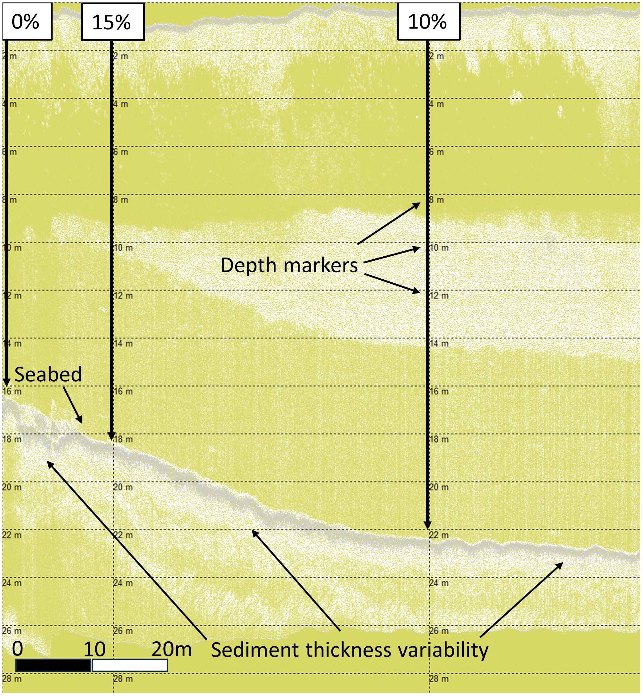
Figure 4 Shapinsay horse mussel (SHH21) SBP HF data.
In analogous research (Sheehy et al., 2024b), in LF3 data the darker grey layer under the seabed was corroborated as the TST from the core data. This layer, with variable sediment thickness can be observed as the horse mussel beds lies across a benthic slope, deepening from left to right in Figure 5. Horse mussel abundance is greatest on this slope, with decreased abundance observed on the shallow shelf on the left (0% to 10% cover from left to right), and the deeper shelf to the right (40% to 10% to 0% cover from left to right).
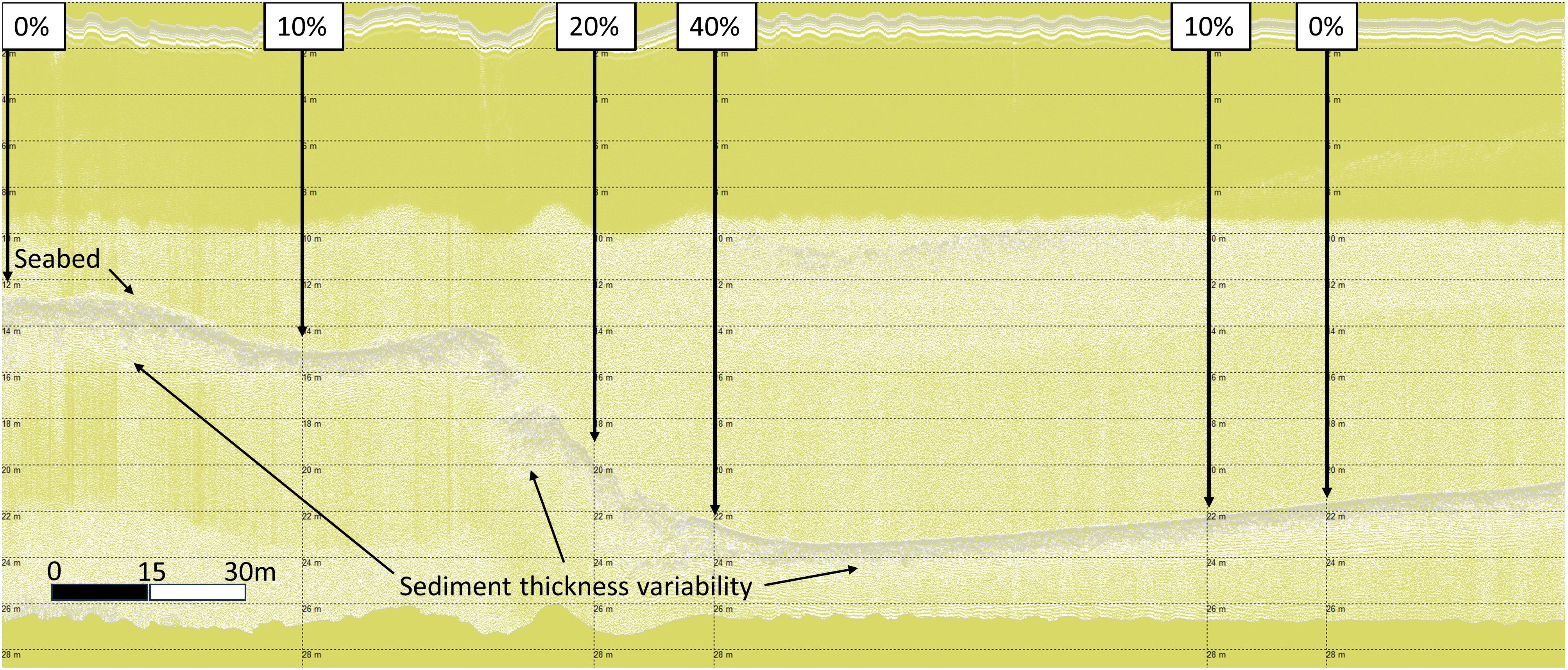
Figure 5 Shapinsay Horse Mussel (SSHH12) SBP LF data with total sediment layer thickness variability.
Bottom tracking, using the ‘threshold detection’ algorithm, was used to detail the seabed in SBP files; blanking, duration, and threshold settings were adjusted per file for best fit. In addition to this reflector for the seabed, first multiples3 and bedrock were also identified and highlighted where applicable to further help with sediment layer identification. Sediment layers were added as acoustic layers within the horse mussel bed survey transect files. Layer sediment thickness with reference to the seabed was determined using the ‘calculate thickness’ feature in Sonarwiz. Data were then exported as a.csv file, with associated horse mussel bed percentage cover and depth and imported back into QGIS. Best available current speed (Almoghayer et al., 2022), and wave exposure (Burrows, 2007) data were matched to SBP ping data by GPS position in QGIS then exported for subsequent analysis in R (R Core Team, 2023). Data points of no horse mussel percentage cover were removed from subsequent analysis. Prior to analysis, variables were tested for covariance and selected based on minimal covariance and/or regional accuracy. Depth and current data were available from UK wide data but data specific to Orkney and the SBP data were selected due to their greater accuracy for the survey site. Covariance and scaled covariance of principal components are provided in the Supplementary Material.
Individual transects were subset for spatial autocorrelation tests then tested sequentially on HF1 channel data; spatial autocorrelation was assumed to be functionally similar between HF1 and LF3 channel data. Subsets of data are labelled by channel (H), sample distance interval in m (1,5,10, or 20), and transect (SHH11, SHH22, SHH31, SHH41, and SHH52). SHH transects had similar results in Moran Monte-Carlo simulations. SHH11 and SHH22 had non-significant spatial autocorrelation at distance sampling interval of 10m whilst SHH31, SHH41, and SHH52 had non-significant spatial autocorrelation at distance sampling intervals of 5m in Moran tests (p > 0.2). Moran Monte-Carlo simulations can be seen in the Supplementary Material.
Given the variability of spatial autocorrelation effects between transects, a sampling distance interval of 10m was set for further analysis of data through Structural Equation Modelling (SEM). SEM was used to determine the relative influences and interactions of abiotic and biotic factors on horse mussel bed sediment thickness.
Final data were comprised of:
• SBP data
o Latitude and Longitude
o Transect identifier
o SBP channel
o Sediment thickness
o Depth (taken from the SBP data and adjusted for tide)
• DDV data
o Horse mussel percentage cover
• Environmental data
o Current speed data in m/s (Almoghayer et al., 2022)
o Wave exposure data as a fetch index (Burrows, 2007)
SEM pathway analysis was used to determine and highlight the distinct effects of abiotic and biotic variables on sediment thickness. For this purpose, SEM pathway analysis is better suited than Generalised Linear Models (GLMs), Generalised Additive Models (GAMs), or other regression as the SEM pathway plots can clearly differentiate the coefficient loadings involved in the analysis and perform potentially independent multiple regressions simultaneously (Nusair and Hua, 2010). SEM pathway analysis undertaken for this study used a priori assumptions that environmental variables determine horse mussel percentage cover, that both environmental variables and percentage cover determine sediment thickness, and that these are one-way relationships, for example, sediment thickness does not determine percentage cover. SEM pathway analysis was conducted using the R package ‘lavaan’ version 0.6-15 (Rosseel et al., 2018). Saturated models (df = 0) were used rather than over-identified models due to subset data limitations given the number of included parameters (Deng et al., 2018). Maximum likelihood with robust standard errors (MLR) was used to deal with non-normality in the data subsets (Fan et al., 2016).
Results
Horse mussel percentage cover and sediment thickness
The mean horse mussel shallow layer sediment thickness was 0.78m (n = 48, SD = 0.21) with a maximum recorded thickness of 1.37m at 10% horse mussel cover. The mean total sediment thickness for horse mussel was 1.32m (n = 48, SD = 0.54) with a maximum recorded thickness of 3.00m at 10% horse mussel cover.
There are limited data for horse mussel percentage cover, with values only recorded from 10% to 40% cover. There is no discernible correlation of horse mussel percentage cover on the SST (HF1) layer sediment thickness. A boxplot of horse mussel percentage cover against sediment layer thickness for both the SST (HF1) and TST (LF3) data is detailed in Figure 6.
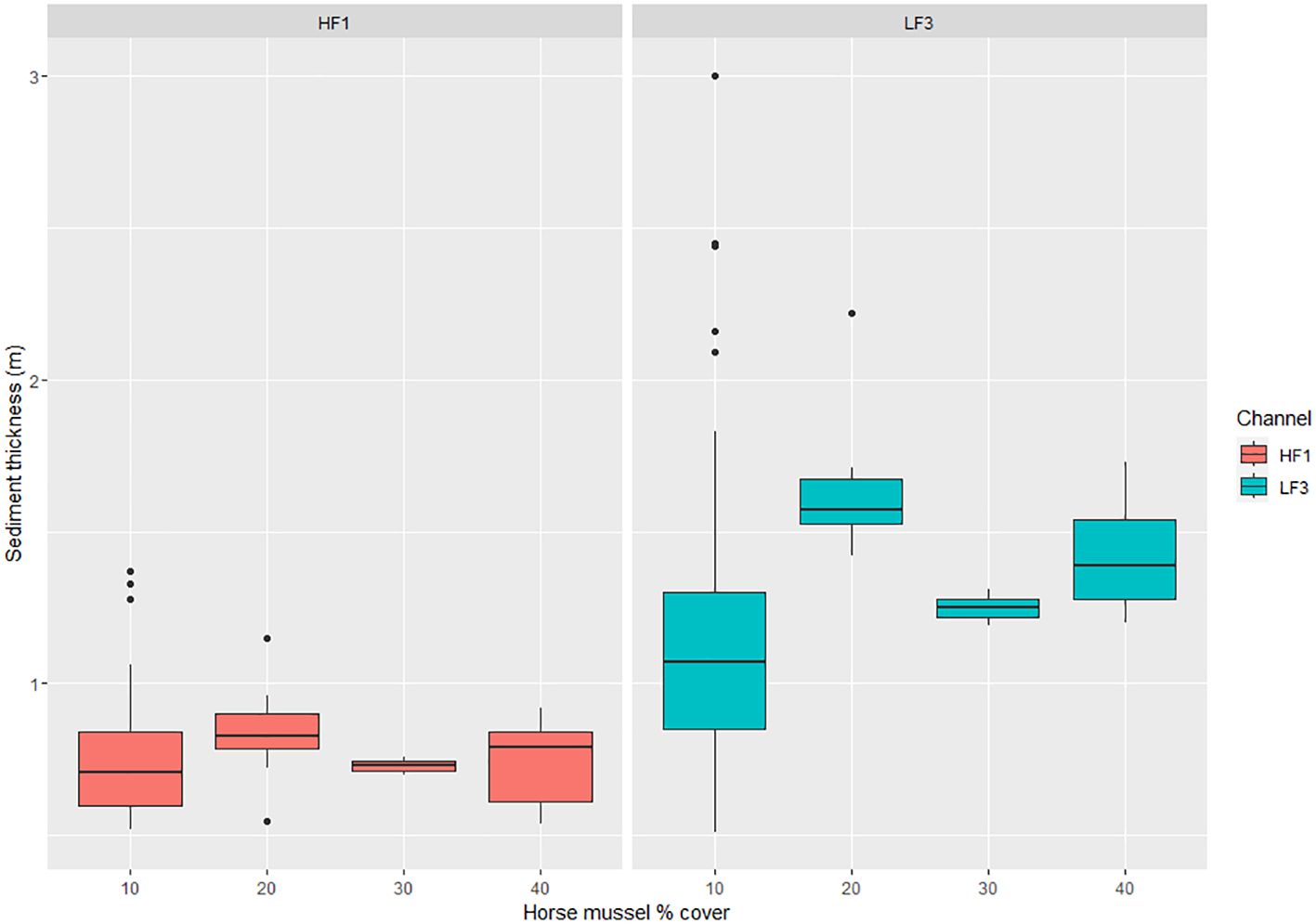
Figure 6 Boxplot of horse mussel percentage cover against Shallow Sediment Thickness (SST) on the HF1 data channel and Total Sediment Thickness (TST) on the LF3 data channel. Sediment thickness (m) is detailed on the y-axis and maerl percentage cover on the x-axis.
Structural equation modelling
Regression coefficients are presented as numbers that signify the relationship between the factor and variable, with significance of effect denoted by *. The SEM shows limited covariance of abiotic variables; depth, current speed, and wave exposure. Horse mussel percentage cover had a significant positive relationship with depth (0.34, p < 0.01). Wave exposure had the most significant abiotic correlation with horse mussel percentage cover, with a significant negative correlation observed (-0.33, p < 0.001). Only depth, with a negative relationship, had a significant correlation with the SST (-0.37, p < 0.001). The TST had significant correlations with all variables. All abiotic variables, depth (-0.25, p < 0.05), current speed (-0.27, p < 0.01), and wave exposure (-0.22, p < 0.05) had significant negative correlations with the TST. Horse mussel percentage cover had a significant positive relationship with the TST (0.22, p < 0.05). There was a significant positive correlation between the SST and the TST (0.40, p < 0.05).
The SEM identifying key relationships between abiotic data, horse mussel percentage cover, and horse mussel sediment thickness, is detailed in Figure 7.
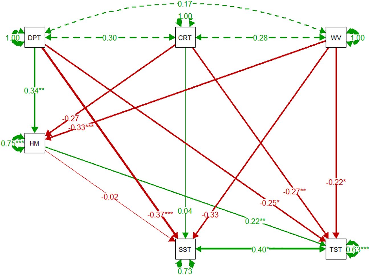
Figure 7 Horse mussel pathway SEMs of environmental variables, horse mussel percentage cover, Shallow Sediment Thickness (SST), and Total Sediment Thickness (TST). Green and red arrows denote positive and negative relationships respectively, dashed arrows represent covariance between exogenous variables. Arrow width denotes the coefficient strength. Circular arrows from each variable represent the residual variance. Coefficient estimate strength is detailed by the number along the arrow, with significance denoted by * p < 0.05, ** p < 001, and *** p < 0.001.
Discussion
Sub-bottom profiling for blue carbon quantification
Review of the horse mussel SBP data alongside analogous research on core ground-truthed seagrass and maerl habitats (Sheehy et al., 20231; Sheehy et al., 2024b) supports SBP data as an acceptable method with which to quantify horse mussel bed sediment thickness. There are similar identifying features of sediment in seagrass, maerl, and horse mussel habitats; bedrock, surface biomass, bands of sediment, and correlated variability of sediment thickness with percentage cover were all identifiable. There are very limited data on horse mussel bed sediment carbon content and thickness. A mean sediment thickness of 0.75m used in most estimates of horse mussel blue carbon research (Burrows et al., 2014, 2017; Porter et al., 2020) is based off only one study which also used acoustic techniques to quantify horse mussel bed sediment thickness (Lindenbaum et al., 2008). We find, however, that a layer of predominantly organic carbon may extend deeper than this to a mean depth of 0.78m, and that total sediment thickness has a mean depth of 1.37m. Without core ground-truthing there is limited certainty in the robustness of these data. Given that previous research used a similar acoustic sounding method, however, they are believed to be as robust as existing estimates for horse mussel bed sediment thickness. Advances in acoustic sounding methods also suggest the data presented in this study are likely to be more robust than those from over 10 years ago. Additionally, horse mussel shell material are particularly robust and estimated to persist for 500-2000 years on the benthic shelf (Smith, 1993). More recent estimates suggest that at the sediment-water interface, total shell dissolution may take centuries to several millennia (Smith and Nelson, 2003). Thick deposits of horse mussel beds and sediment may therefore have the potential to sequester carbon over timescales of ~1000 years (Burrows et al., 2014) and support conclusions of >1m horse mussel sediment thickness from SBP analysis.
Determining abiotic and biotic influences on maerl sediment thickness
The Shapinsay horse mussel site is believed to be a typical horse mussel site; a typical horse mussel bed site is characterised with a mixed sediment substrate (BGS, 2019), suitable environmental parameters such as relatively shallow depths < 50m (Hiscock et al., 2004), and with associated flora and fauna as defined in JNCC biotopes (JNCC, 2023). As such, analysis of this site is believed to be a good example of typical horse mussel beds in Orkney and Scotland. To be more specific, however, and consider the Shapinsay site as a defined biotope, the Shapinsay site details a sparse horse mussel bed habitat (JNCC, 2022d). The range of horse mussel percentage cover only extends from 10% to 40%; the data therefore don’t capture the full range of horse mussel habitat condition or the biotopes of abundant (JNCC, 2022b) or super-abundant (JNCC, 2022a) horse mussel populations. The limited data may therefore occlude wider trends of the data or extrapolation of data, and sediment thickness, to horse mussel beds with greater abundance.
The SEM details the significance of depth and wave exposure on horse mussel abundance. This matches expected deterministic effects on horse mussel habitat based on known environmental parameters (Hiscock et al., 2004), though it is unclear why no significance of effect was observed for current speed. This could be due to limitations in data, with data all taken from one site with limited abiotic variability, but then non-significance for depth and wave exposure would also be reasonably expected. Only depth was found to be significant in structuring the SST. This could be due to a compression of the perceived sediment layer signal in the SBP data with increased depth, thereby just reflecting a difference of SBP signal noise rather than sediment thickness at different depths. Given variability of depth on sediment thickness observed in analogous research however (Sheehy et al., 20231; Sheehy et al., 2024b), it is more likely to be due to associated reduction of OC production from the horse mussel bed and associated fauna and flora, regardless of horse mussel abundance, in the horse mussel bed at greater depths. In other contemporary shellfish literature, in shallow subtidal reefs, there is more effective drawdown of atmospheric CO2 through filtration and ‘rapid biodeposition of carbon-fixing primary producers’ (Fodrie et al., 2017). Depth had a similar, but slightly weaker relationship with the TST, this is again expected to be due to differences in OC production at depth; a thicker SST will also increase the TST which was also a significant correlation in the SEM. The absence of bioeroders such as endolithic algae and limpets in deeper waters past the euphotic zone can also lead to a greater resilience of IC in shell material in deeper waters (Akpan and Farrow, 1985). Current speed and wave exposure were found to be a significant factor on horse mussel bed TST. The negative correlations are expected with less sediment deposition, or retention, in areas with greater hydrodynamics leaving a thinner sediment. Horse mussel percentage cover was found to be non-significant with the SST. This may suggest associated fauna and flora have a greater contribution to organic production and sediment carbon sequestration than the horse mussel bed itself. It is, however, unclear if there is a threshold of minimum horse mussel abundance for this effect to occur, if partial/degraded horse mussel habitats provide sufficient habitat for associated fauna and flora, or if horse mussel production was not evident due to abundance data limitations. For the TST, horse mussel percentage cover was found to be significant and positively correlated. This may be the result of horse mussel beds sequestering more IC than OC, the diagenesis of OC over time leaving less OC at greater sediment depths, or a mixture of these factors. Hypoxia is strongly significant in determining rates of diagenesis in blue carbon sediments (Fourqurean and Schrlau, 2003; Kennedy et al., 2010; Pedersen et al., 2011). The speed of deposition will therefore contribute to thicker sediment stocks and increase burial, and reduce diagenesis, of sedimentary OC.
Uncertainties
DDV footage was used to detail horse mussel percentage cover as a cost-effective and applicable small to medium scale survey method. It may not, however, be as accurate as in-situ methods using transects or quadrats. Given the fine scale variation at which horse mussel bed density occurs (Lindenbaum et al., 2008) and difficulty of live/dead horse mussel identification (Hirst et al., 2012; Moore et al., 2013), DDV data may not be sufficient to accurately characterise horse mussel habitat condition. Specific to this study, with the horse mussel site situated on a steep slope, this creates additional problems for surveying, with a more variable camera angle which also subsequently affects lighting and accurate identification of abundance. There is therefore a potential for observer bias and inaccurate recording of percentage cover with specific locations. The scale of the survey, interpolation, and removal of data points with no horse mussel cover values, are believed to be suitable mitigation for this potential uncertainty. There is a potential issue with interpolation of percentage cover between point locations, but, whilst other acoustic methods may be able to map horse mussel habitats (Wildish et al., 1998; Lindenbaum et al., 2008), these require ground truthing with visual data. Acoustic methods are also unable to characterise habitat abundance.
Considering the spatial distribution of the Shapinsay horse mussel bed survey site, it is also understood that the site might experience anthropogenic disturbance due to fishing; the site is not within the bounds of any protected areas (JNCC, 2022c). If collocated commercial species are associated along a specific gradient of environmental variables, this may then also structure disturbance, and horse mussel abundance, along spatial gradients. Horse mussel habitat is particularly susceptible to dredging, trawling, and associated smothering from resuspended sediment (Strain et al., 2012; Cook et al., 2013; Fariñas-Franco et al., 2018; Marine Scotland, 2018). The associated faunal communities, important to carbon sequestration processes, are less tolerant of this type of impact than the horse mussels; horse mussel have some capacity of movement through smothering sediment accretions (Magorrian and Service, 1998). It is unclear, however, on the degree of disturbance this site experiences, and the extent of disturbance on site horse mussel habitat condition, associated fauna and flora, and sediment deposition. The horse mussel site is most abundant on a relatively steep slope, with the upper and lower plateaus with less percentage cover (see Figures 4 and 5). This slope may therefore offer protection from dredging and trawling disturbance, with greater disturbance on shallower and deeper plateaus adjacent to the slope. Given the key connections of habitat condition, associated biodiversity, and carbon sequestration these effects may alter the results beyond that which can be accounted for with the included variables. Whilst disturbance will alter the composition of live and dead horse mussels in the habitat, and future carbon sequestration, it is unclear on how this might affect existing (deeper) sediment stocks; the level of disturbance may be negligible on horse mussel sediments or create significant loss through oxidation of previously anoxic sediments (Fourqurean and Schrlau, 2003; Kennedy et al., 2010; Pedersen et al., 2011). Anthropogenic disturbance may also affect carbon fluxes, with import of allochthonous carbon and export of autochthonous carbon. Disturbance may create localised differences in carbon fluxes with subsequent effects on sediment deposition speeds and sediment thickness.
Unfortunately, the lack of core data specifically linked to this horse mussel site, and the limited range of data, create greater uncertainty into the robustness of horse mussel layer identification through SBP data. In analogous research, core data allowed specific matching of the SST and the TST (Sheehy et al., 20231; Sheehy et al., 2024b), which was then extrapolated to horse mussel sediments. Aligned with other research that uses acoustic sounding techniques to determine horse mussel sediment extents (Lindenbaum et al., 2008), this is believed to be a robust approach, but may not be as robust for carbon accreditation processes as those linked to core verified sediment thickness (Sheehy et al., 2024a). The SBP settings used to identify horse mussel bed sediment may be specifically aligned to horse mussel habitats in Orkney, and it is unclear how readily they might be extrapolated across the UK given the range and variability of horse mussel habitats across the UK (Fariñas-Franco et al., 2023). Future research using SBP data for blue carbon quantification would likely have to align SBP data with local cores.
Finally, residual variance in sediment thickness observed in the SEM analysis also suggests there are key deterministic factors that were outside of the scope of this research; this may include other abiotic data such as geological effects (Bates et al., 2014) terrigenous/allochthonous inputs (Bosence and Wilson, 2003; Mao et al., 2020), and other measures of biodiversity (Bosence, 1976; Hall-Spencer and Atkinson, 1999).
Future research
Whilst this study furthers understanding of horse mussel habitats, it also highlights some key data gaps in horse mussel research. When addressed, within the context of blue carbon research, they might provide a sufficient knowledge base, data, and approach to support cost-effective quantification of horse mussel bed carbon stocks. This may support subsequent accreditation of that carbon, and wider implementation of blue carbon as a tool for climate change mitigation and adaptation.
At the research level, there is a significant data gap in carbon content for horse mussel sediments, with only one study using a shallow grab sample (Collins, 1986), from which data have been extrapolated to deeper sediments and other horse mussel habitats. Given the lack of core data, there are also no data to be able to directly link changes in horse mussel sediment composition across sediment depths; this is commonly observed in marine sediments (Bates et al., 2014; Sheehy et al., 20231; Sheehy et al., 2024b). Cores of horse mussel sediments, aligned with SBP data, and robust measures of habitat condition would reinforce an integrated approach to blue carbon habitat condition and carbon stocks. It would also resolve issues around limited data in this and wider studies.
Considering financial and logistical constraints inherent in blue carbon science (Sheehy et al., 2024a), the integrated approach of core, SBP, DDV, and abiotic data presented in this study is essential to robust and cost-effective large-scale quantification of horse mussel bed carbon stocks and sequestration potential. This approach may be reflected in wider blue carbon science, applicable to other habitats and species (Sheehy et al., 20231; Sheehy et al., 2024b), in addition to potentially supporting the evaluation and valuation of unvegetated stocks of marine sediment carbon (Hunt et al., 2021; Smeaton et al., 2021; Sheehy et al., 2024a). The resultant increased knowledge base from such research may also be used to support and align machine learning and predictive modelling to further support more cost-effective large-scale blue carbon quantification.
The integrated approach of horse mussel bed analysis through core, SBP, DDV, and abiotic data is also framed within an eco-social economics framework for climate change mitigation and adaptation (Sheehy et al., 2024a). A robust dataset, including respiration and calcification processes (Lee et al., 2024), of horse mussel bed sediments supports carbon accreditation processes and inclusion in blue carbon policy frameworks. In turn these can provide tangible benefits and incentives for policy makers and local communities to take a pro-active approach to blue carbon protection and restoration. The benefits promote social well-being and, especially when aligned to measures of habitat condition, also encourage ecological values; ecological values may also be bolstered by financing available for biodiversity targets and other measures of ecosystem service evaluation (Sheehy et al., 2024a). Together, this approach aligns to best understanding of effective ecological protection, blue carbon science, societal engagement, and economic support to drive climate change mitigation and adaptation.
Within a framework that uses SEM, future models may incorporate wider abiotic and biotic data to further refine understanding of the links between abiotic factors, horse mussel habitat condition, and sediment thickness and composition. Considering ecosystem service value and accreditation criteria, latent SEM may use a similar structure to that detailed in Figure 8. This SEM approach can link a wider range of abiotic data that might be suitable at large scale, to a multitude of biotic data, ecosystem service value, accreditation criteria, and carbon credit value based on tier level assessment. Alternatively, latent variables could be structured to include calcification and respiration processes (Lee et al., 2024) determine whether the horse mussel bed acts as a carbon source or sink (Fodrie et al., 2017).
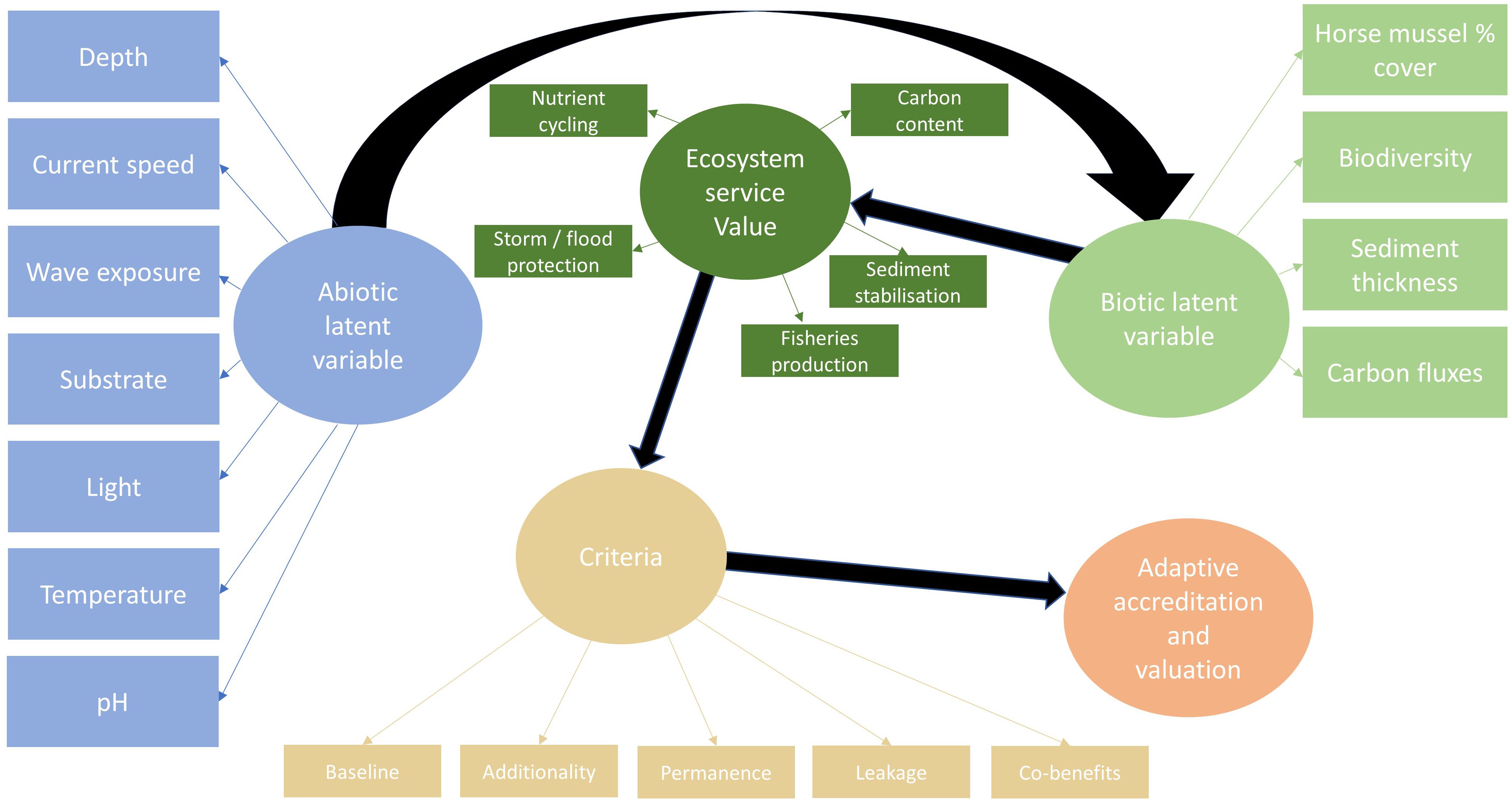
Figure 8 Horse mussel SEM for machine learning techniques to link abiotic and biotic factors to carbon accreditation criteria, adaptive valuation, and total economic value.
Conclusions
Primarily, this study evaluates the use of SBP data to identify and determine horse mussel bed sediment thickness. This study details how horse mussel sediment layers can be robustly identified with SBP data; this supplements previous estimations of horse mussel sediment thickness using acoustic techniques (Lindenbaum et al., 2008). Subsequently, this study significantly updates those previous estimates of horse mussel bed sediment thickness from a mean sediment thickness of 0.75m to 1.37m. This study therefore has the potential to almost double previous estimates of horse mussel carbon stocks; horse mussel sediment thickness has generally been assumed to be a mean thickness of 0.75m (Burrows et al., 2017; Porter et al., 2020). Whilst there is still no route for accreditation of horse mussel carbon into markets, and uncertainty on the application of accreditation to blue carbon sediment thickness greater than 1m (Sheehy et al., 2024a), this study highlights the large potential of horse mussel beds for carbon sequestration. As such, it furthers the evidence base to support the inclusion of horse mussels as a blue carbon habitat in policy frameworks (IPCC, 2014; Lovelock and Duarte, 2019; Sheehy et al., 2024a).
Key abiotic factors on horse mussel percentage cover are also identified, with depth and wave exposure found to be the most deterministic. This study finds that both abiotic factors and horse mussel habitat condition (based on horse mussel percentage cover) are deterministic factors in the extents of underlying sedimentary carbon stocks; this supports existing research that details the importance of habitat condition on carbon sequestration potential (Sanderson et al., 2014; Mackenzie et al., 2018). This is the only research, to the authors’ knowledge, that quantifies the effect of habitat condition (using percent coverage of the habitat forming species) on horse mussel bed sediments and carbon stocks. Subsequently, carbon sequestration potential, and the associated biodiversity of the horse mussel habitat linked to horse mussel habitat condition, are key considerations of blue carbon framed horse mussel research. Considering the wider context of blue carbon policy and eco-social economics, this study then reinforces the integration of habitat condition and associated biodiversity values and ecological conservation with economic value and climate change mitigation (WWF, 2022).
Finally, this study details an integrated approach to blue carbon quantification that uses core, SBP, DDV, and abiotic data. This approach considers key considerations of future research for cost-effective and applicable survey methods at small to medium scales, from 0.05-1 km2 ranges (Malerba et al., 2023). This approach also links to future research of blue carbon stock estimation at large scales using predictive modelling, by providing data that can be used in stacked species distribution models (Pinto-Ledezma and Cavender-Bares, 2021) and scaled to abundance predictions (Sheehy et al., 20234). This study therefore also considers the financial and logistical constraints of future research agendas (Macreadie et al., 2014), ecological values of blue carbon habitats beyond carbon sequestration (Fodrie et al., 2017), and supports blue carbon science within the wider policy context of eco-social economics (Sheehy et al., 2024a).
Data availability statement
The raw data supporting the conclusions of this article will be made available by the authors, without undue reservation.
Author contributions
JS: Conceptualization, Data curation, Formal analysis, Funding acquisition, Investigation, Methodology, Project administration, Resources, Software, Validation, Visualization, Writing – original draft, Writing – review & editing. RB: Formal analysis, Methodology, Resources, Software, Supervision, Validation, Writing – review & editing. MB: Investigation, Supervision, Validation, Writing – review & editing. JP: Investigation, Supervision, Validation, Writing – review & editing.
Funding
The author(s) declare financial support was received for the research, authorship, and/or publication of this article. This work was supported by the Natural Environment Research Council [grant number NE/S007342/1]. This research was also supported by grants from Marine Alliance for Science and Technology for Scotland (MASTS) Biogeochemistry Forum, MASTS Coastal Forum, and Sea-Changers. Survey data were also made available with the help of MASTS vessel time.
Acknowledgments
The authors would like to acknowledge the support of Marine Alliance for Science and Technology Scotland (MASTS) and associated forums, the Scottish Universities Partnership for Environmental Research Doctoral Training Partnership (SUPER DTP), and Sea Changers for all their help.
Conflict of interest
The authors declare that the research was conducted in the absence of any commercial or financial relationships that could be construed as a potential conflict of interest.
The reviewer JF-F declared a past co-authorship with the author JP to the handling editor.
Publisher’s note
All claims expressed in this article are solely those of the authors and do not necessarily represent those of their affiliated organizations, or those of the publisher, the editors and the reviewers. Any product that may be evaluated in this article, or claim that may be made by its manufacturer, is not guaranteed or endorsed by the publisher.
Supplementary material
The Supplementary Material for this article can be found online at: https://www.frontiersin.org/articles/10.3389/fmars.2024.1321366/full#supplementary-material
Footnotes
- ^ Sheehy, J., Porter, J. S., Bell, M. C., and Bates, R. (2023). Seagrass: sounding out sediment thickness. (Manuscript submitted for publication).
- ^ MacLeod, A. M. (2015). The Blue carbon potential of Maerl in the Wyre Sound MPA, Orkney. (Unpublised MSc thesis).
- ^ First multiples are reflections of the SBP pings hitting the seafloor repeated at twice the travel time to reach the seafloor. These were identified by selecting m/s travel time annotation in the preferences of image analysis in Sonarwiz.
- ^ Sheehy, J. M., Porter, J., Bell, M. C., and Kerr, S. (2023). Adaptive multistacked species distribution modelling for blue carbon quantification. (Manuscript submitted for publication).
References
Akpan E.B., Farrow G. E. (1985). Shell bioerosion in high-latitude low-energy environments: Firths of Clyde and Lorne, Scotland. Mar. Geol. 67, 139–150. doi: 10.1016/0025-3227(85)90152-5
Almoghayer M. A., Woolf D. K., Kerr S., Davies G. (2022). Integration of tidal energy into an island energy system – A case study of Orkney islands. Energy 242. doi: 10.1016/j.energy.2021.122547
Armstrong S., Hull S., Pearson Z., Wilson R., Kay S. (2020) Estimating the Carbon Sink Potential of the Welsh Marine Environment (Cardiff: NRW). Available at: https://cdn.naturalresources.wales/media/692035/nrw-evidence-report-428_blue-carbon_v11-002.pdf (Accessed 26 October 2022).
Bates M., Bates R., Frew C., Huws D., Nayling N., Dawson S., et al. (2014) Bay of Firth (Orkney: coring report). Available at: https://www.abdn.ac.uk/staffpages/uploads/arc007/Rising_Tide_Coring_report_2014_.pdf (Accessed 14 April 2022).
BGS. (2019). British Geological Survey - UK ContShelf BGS 1:1M Seabed Sediments (BGS WMS). Available at: http://ogc.bgs.ac.uk/cgi-bin/BGS_Bedrock_and_Superficial_Geology/wms.
Bosence D. W. J. (1976). Ecological studies on two carbonate sediment producing coralline algae from western Ireland. In: Palaeontology. Available at: https://www.palass.org/sites/default/files/media/publications/palaeontology/volume_19/vol19_part2_pp365-395.pdf (Accessed 25 February 2022).
Bosence D., Wilson J. (2003). “Maerl growth, carbonate production rates and accumulation rates in the northeast Atlantic,” in Aquatic Conservation: Marine and Freshwater Ecosystems (John Wiley & Sons, Ltd), S21–S31. doi: 10.1002/aqc.565
Burrows M. T. (2007). Wave Fetch Model. Wave Fetch Model. Available at: https://www.sams.ac.uk/people/researchers/burrows-professor-michael/ (Accessed 24 January 2023).
Burrows M. T., Kamenos N. A., Hughes D. J., Stahl H., Howe J. A., Tett P. (2014). Assessment of carbon budgets and potential blue carbon stores in Scotland’s coastal and marine environment. Project Report. Scottish Natural Heritage Commissioned Report No. 761. (Scottish Natural Heritage in Inverness), Vol. 7. 90, pp.
Burrows M. T., Hughes D. J. J., Austin W. E. N. E. N., Smeaton C., Hicks N., Howe J. A. A., et al. (2017) Assessment of Blue Carbon Resources in Scotland’s Inshore Marine Protected Area Network. Scottish Natural Heritage Commissioned Report No. 957 (Scottish Natural Heritage Commissioned Report). Available at: https://www.nature.scot/sites/default/files/Publication2017-SNHCommissionedReport957-AssessmentofBlueCarbonResourcesinScotland%27sInshoreMarineProtectedAreaNetwork.pdf (Accessed 13 November 2019).
Chesapeake Technology (2023) SonarWiz Sub-bottom | Collection & Processing | Chesapeake Technology. Available at: https://chesapeaketech.com/products/sonarwiz-sub-bottom/ (Accessed 15 March 2023).
Collins M. J. (1986) Taphonomic processes in a deep water Modiolus-brachiopod assemblage from the west coast of Scotland. Available at: https://eleanor.lib.gla.ac.uk/record=b1267525 (Accessed 27 October 2022).
Cook R., Fariñas-Franco J. M., Gell F. R., Holt R. H. F., Holt T., Lindenbaum C., et al. (2013). The Substantial first impact of bottom fishing on rare biodiversity hotspots: A dilemma for evidence-based conservation. PloS One 8, e69904. doi: 10.1371/journal.pone.0069904
Deng L., Yang M., Marcoulides K. M. (2018). Structural equation modeling with many variables: A systematic review of issues and developments. Front. Psychol. 9. doi: 10.3389/fpsyg.2018.00580
Fan Y., Chen J., Shirkey G., John R., Wu S. R., Park H., et al. (2016). Applications of structural equation modeling (SEM) in ecological studies: an updated review. Ecol. Processes 5, 1–12. doi: 10.1186/s13717-016-0063-3. Springer Verlag.
Fariñas-Franco J. M., Allcock A. L., Roberts D. (2018). Protection alone may not promote natural recovery of biogenic habitats of high biodiversity damaged by mobile fishing gears. Mar. Environ. Res. 135, 18–28. doi: 10.1016/j.marenvres.2018.01.009
Fariñas-Franco J. M., Pearce B., Porter J., Harries D., Mair J. M., Woolmer A. S., et al. (2014) Marine Strategy Framework Directive Indicators for Biogenic Reefs formed by Modiolus modiolus, Mytilus edulisand Sabellaria spinulosa, JNCC Report. Available at: https://data.jncc.gov.uk/data/82ff709f-56ff-4850-bdbf-2a3b63fc8cdc/JNCC-Report-523-FINAL-WEB.pdf (Accessed 20 October 2022).
Fariñas-Franco J. M., Cook R. L., Gell F. R., Harries D. B., Hirst N., Kent F., et al. (2023). Are we there yet? Management baselines and biodiversity indicators for the protection and restoration of subtidal bivalve shellfish habitats. Sci. Total Environ. 863, 161001. doi: 10.1016/j.scitotenv.2022.161001
Fodrie F. J., Rodriguez A. B., Gittman R. K., Grabowski J. H., Lindquist N. L., Peterson C. H., et al. (2017). Oyster reefs as carbon sources and sinks. Proc. R. Soc. B: Biol. Sci. 284. doi: 10.1098/rspb.2017.0891
Fourqurean J. W., Schrlau J. E. (2003). Changes in nutrient content and stable isotope ratios of C and N during decomposition of seagrasses and mangrove leaves along a nutrient availability gradient in Florida Bay, USA. Chem. Ecol. 19, 373–390. doi: 10.1080/02757540310001609370
Hall-Spencer J. M., Atkinson R. J. A. (1999). Upogebia deltaura (Crustacea: Thalassinidea) in Clyde Sea maerl beds, Scotland. J. Mar. Biol. Assoc. United Kingdom 79, 871–880. doi: 10.1017/S0025315498001039
Hirst N. E., Clark L., Sanderson W. G. (2012). The distribution of selected MPA search features and Priority Marine Features off the NE coast of Scotland. Scottish Natural Heritage Rep. 500, 132.
Hiscock K., Southward A., Tittley I., Hawkins S. (2004). Effects of changing temperature on benthic marine life in Britain and Ireland. Aquat. Conservation: Mar. Freshw. Ecosyst. 14, 333–362. doi: 10.1002/aqc.628
Holt T. J., Rees E. I., Hawkins S. J., Seed R. (1998) Biogenic Reefs (volume IX). An overview of dynamic and sensitivity characteristics for conservation management of marine SACs. Scottish Association for Marine Science (UK Marine SACs Project). Available at: http://ukmpa.marinebiodiversity.org/uk_sacs/pdfs/biogreef.pdf (Accessed 19 October 2022).
Howard J., Hoyt S., Isensee K., Pidgeon E., Telszewski M. (2014) Coastal Blue Carbon: Methods for Assessing Carbon Stocks and Emissions Factors in Mangroves, Tidal Salt Marshes, and Seagrass Meadows (Arlington, Virginia, USA.: Conservation International, Intergovernmental Oceanographic Commission of UNESCO, International Union for Conservation of Nature). Available at: https://www.thebluecarboninitiative.org/manual (Accessed 7 November 2019).
Hunt C., Demšar U., Dove D., Smeaton C., Cooper R., Austin W. E. N. N. (2020). Quantifying marine sedimentary carbon: A new spatial analysis approach using seafloor acoustics, imagery, and ground-truthing data in scotland. Front. Mar. Sci. 7. doi: 10.3389/fmars.2020.00588
Hunt C. A., Demšar U., Marchant B., Dove D., Austin W. E. N. (2021). Sounding out the carbon: the potential of acoustic backscatter data to yield improved spatial predictions of organic carbon in marine sediments. Front. Mar. Sci. 8, 1684. doi: 10.3389/fmars.2021.756400
Innomar. (2023). SES-Convert Data Converter - Innomar. Available at: https://www.innomar.com/products/innomar-software/ses-convert-data-converter (Accessed 30 March 2023).
IPCC (2014). 2013 Supplement to the 2006 IPCC Guidelines for National Greenhouse Gas Inventories: Wetlands. (Switzerland: Intergovernmental Panel on Climate Change). doi: 10.1038/ngeo1123
JNCC (2019) UK BAP Priority Species | JNCC - Adviser to Government on Nature Conservation. Available at: https://jncc.gov.uk/our-work/uk-bap-priority-habitats/ (Accessed 18 October 2022).
JNCC (2022a) Modiolus modiolus beds on open coast circalittoral mixed sediment - JNCC Marine Habitat Classification, The Marine Habitat Classification for Britain and Ireland Version 22.04. Available at: https://mhc.jncc.gov.uk/biotopes/jnccmncr00001097 (Accessed 20 February 2023).
JNCC (2022b) Modiolus modiolus beds with hydroids and red seaweeds on tide-swept circalittoral mixed substrata - JNCC Marine Habitat Classification, The Marine Habitat Classification for Britain and Ireland Version 22.04. Available at: https://mhc.jncc.gov.uk/biotopes/jnccmncr00000657 (Accessed 20 February 2023).
JNCC (2022c) MPA Mapper | JNCC - Adviser to Government on Nature Conservation, Microsoft corporation earthstar geographics SIO. Available at: https://jncc.gov.uk/mpa-mapper/ (Accessed 18 October 2022).
JNCC (2022d) Sparse Modiolus modiolus, dense Cerianthus lloydii and burrowing holothurians on sheltered circalittoral stones and mixed sediment - JNCC Marine Habitat Classification, The Marine Habitat Classification for Britain and Ireland Version 22.04. Available at: https://mhc.jncc.gov.uk/biotopes/jnccmncr00000668 (Accessed 20 February 2023).
JNCC (2023) Marine Habitat Classification for Britain and Ireland (22.04): Overview of changes since MHCBI 15.03. Available at: https://hub.jncc.gov.uk/assets/f9a6a2be-e6be-4f7f-8605-28c1b4062658 (Accessed 28 November 2017).
Jones L. A., Hiscock K., Connor D. W. (2000) Marine habitat reviews. A summary of ecological requirements and sensitivity characteristics for the conservation and management of marine SACs. Peterborough, Joint Nature Conservation Committee. (UK Marine SACs Project report.). Available at: http://ukmpa.marinebiodiversity.org/pdf/Summary_documents/marine-habitats-review.pdf (Accessed 25 October 2022).
Kennedy H., Beggins J., Duarte C. M., Fourqurean J. W., Holmer M., Marbá N., et al. (2010). Seagrass sediments as a global carbon sink: Isotopic constraints. Global Biogeochemical Cycles 24. doi: 10.1029/2010GB003848
Kent F. E. A., Mair J. M., Newton J., Lindenbaum C., Porter J. S., Sanderson W. G. (2017). Commercially important species associated with horse mussel (Modiolus modiolus) biogenic reefs: A priority habitat for nature conservation and fisheries benefits. Mar. pollut. Bull. 118, 71–78. doi: 10.1016/j.marpolbul.2017.02.051
Lee H. Z. L., Davies I. M., Baxter J. M., Diele K., Sanderson W. G. (2024). A blue carbon model for the European flat oyster (Ostrea edulis) and its application in environmental restoration. Aquat. Conservation: Mar. Freshw. Ecosyst 34 (1). doi: 10.1002/aqc.4030
Lindenbaum C., Bennell J. D., Rees E. I. S., Mcclean D., Cook W., Wheeler A. J., et al. (2008). Small-scale variation within a Modiolus modiolus (Mollusca: Bivalvia) reef in the Irish Sea: I. Seabed mapping and reef morphology. J. Mar. Biol. Assoc. United Kingdom 88, 133–141. doi: 10.1017/S0025315408000374
Lo Iocano C., Mateo M. A., Gràcia E., Guasch L., Carbonell R., Serrano L., et al. (2008). Very high-resolution seismo-acoustic imaging of seagrass meadows (Mediterranean Sea): Implications for carbon sink estimates. Geophysical Res. Lett. 35. doi: 10.1029/2008GL034773
Lovelock C. E., Duarte C. M. (2019). Dimensions of blue carbon and emerging perspectives. Biol. Lett. 15, 23955–26900. doi: 10.1098/rsbl.2018.0781
Mackenzie C., Kent F. E.A., J.M. B., Porter J. S. (2018). SNH Research Report 1000: Genetic analysis of horse mussel bed populations in Scotland. Scottish Natural Heritage in Inverness.
Macreadie P. I., Baird M. E., Trevathan-Tackett S. M., Larkum A. W. D., Ralph P. J. (2014). Quantifying and modelling the carbon sequestration capacity of seagrass meadows - A critical assessment. Mar. pollut. Bull. 83, 430–439. doi: 10.1016/j.marpolbul.2013.07.038
Magorrian B. H., Service M. (1998). Analysis of underwater visual data to identify the impact of physical disturbance on horse mussel (Modiolus modiolus) beds. Mar. pollut. Bull. 36, 354–359. doi: 10.1016/S0025-326X(97)00192-6
Mainwaring K., Tillin H., Tyler-Walters H. (2014) Assessing the sensitivity of blue mussel beds to pressures associated with human activities. Peterborough, Joint Nature Conservation Committee, JNCC Report No. 506. Available at: https://data.jncc.gov.uk/data/c1a80fb6-ac64-4a9c-aa13-2ab7a441937a/JNCC-Report-506-FINAL-WEB.pdf (Accessed 27 October 2022).
Malerba M. E., Duarte de Paula Costa M., Friess D. A., Schuster L., Young M. A., Lagomasino D., et al. (2023). Remote sensing for cost-effective blue carbon accounting. Earth-Science Rev. 238, 104337. doi: 10.1016/j.earscirev.2023.104337
Mao J., Burdett H. L., McGill R. A. R. R., Newton J., Gulliver P., Kamenos N. A. (2020). Carbon burial over the last four millennia is regulated by both climatic and land use change. Global Change Biol. 26, 2496–2504. doi: 10.1111/gcb.15021
Marine Scotland (2018). PRIORITY MARINE FEATURE (PMF)-FISHERIES MANAGEMENT REVIEW Feature HORSE MUSSEL BEDS.
Monnier B., Pergent G., Mateo M. Á., Carbonell R., Clabaut P., Pergent-Martini C. (2021). Sizing the carbon sink associated with Posidonia oceanica seagrass meadows using very high-resolution seismic reflection imaging. Mar. Environ. Res. 170, 105415. doi: 10.1016/j.marenvres.2021.105415
Moore C. G., Harries D. B., Cook R. L., Hirst N. E., Saunders G. R., Kent F. E. A., et al. (2013) NatureScot Commissioned Report 566: The distribution and condition of selected MPA search features within Lochs Alsh, Duich, Creran and Fyne, Scottish Natural Heritage Commissioned Report. Available at: https://www.nature.scot/doc/naturescot-commissioned-report-566-distribution-and-condition-selected-mpa-search-features-within (Accessed 25 November 2019).
Navarro J. M., Thompson R. J. (1996). Physiological energetics of the horse mussel Modiolus modiolus in a cold ocean environment. Mar. Ecol. Prog. Ser. 138, 135–148. doi: 10.3354/meps138135
NBN (2017) National Biodiversity Network. Available at: https://scotland.nbnatlas.org/ (Accessed 1 August 2018).
Nusair K., Hua N. (2010). Comparative assessment of structural equation modeling and multiple regression research methodologies: E-commerce context. Tourism Manage. 31, 314–324. doi: 10.1016/j.tourman.2009.03.010
OBIS (2022) Ocean Biodiversity Information System - Modiolus modiolus (Linnaeus 1758). Available at: https://obis.org/taxon/140467 (Accessed 18 October 2022).
Ospar Commission (2021) List of Threatened and/or Declining Species & Habitats | OSPAR Commission. Available at: https://www.ospar.org/work-areas/bdc/species-habitats/list-of-threatened-declining-species-habitats (Accessed 18 October 2022).
Pedersen M.Ø., Serrano O., Mateo M. Á., Holmer M. (2011). Temperature effects on decomposition of a Posidonia oceanica mat. Aquat. Microbial Ecol. 65, 169–182. doi: 10.3354/ame01543
Pinto-Ledezma J. N., Cavender-Bares J. (2021). Predicting species distributions and community composition using satellite remote sensing predictors. Sci. Rep. 11, 1–12. doi: 10.1038/s41598-021-96047-7
Porter J., Austin W., Burrows M., Clarke D., Davies G., Kamenos N., et al. (2020). Blue carbon audit of Orkney waters (Scottish Marine and Freshwater Science). Marine Scotland Science. doi: 10.7489/12262-1
Potouroglou M., Whitlock D., Milatovic L., MacKinnon G., Kennedy H., Diele K., et al. (2021). The sediment carbon stocks of intertidal seagrass meadows in Scotland. Estuarine Coast. Shelf Sci. 258, 107442. doi: 10.1016/j.ecss.2021.107442
QGIS (2023) QGIS Geographic Information System (QGIS Association). Available at: https://qgis.org/en/site/ (Accessed 1 August 2018).
Ragnarsson S. A., Burgos J. M. (2012). Separating the effects of a habitat modifier, Modiolus modiolus and substrate properties on the associated megafauna. J. Sea Res. 72, 55–63. doi: 10.1016/j.seares.2012.05.011
R Core Team. (2023). R: A language and environment for statistical ## computing (Vienna, Austria: R Foundation for Statistical Computing). Available at: https://www.r-project.org/.
Rees I. (2009). Background document for Modiolus modiolus beds, OSPAR Commission Biodiversity Series. Available at: https://qsr2010.ospar.org/media/assessments/Species/P00425_Modiolus.pdf (Accessed 18 October 2022).
Ricart A. M., Pérez M., Romero J. (2017). Landscape configuration modulates carbon storage in seagrass sediments. Estuarine Coast. Shelf Sci. 185, 69–76. doi: 10.1016/j.ecss.2016.12.011
Röhr M. E., Holmer M., Baum J. K., Björk M., Chin D., Chalifour L., et al. (2018). Blue carbon storage capacity of temperate eelgrass (Zostera marina) meadows. Global Biogeochemical Cycles 32, 1457–1475. doi: 10.1029/2018GB005941
Rosseel Y., Oberski D., Byrnes J., Vanbrabant L., Savalei V., Merkle E., et al. (2018). Latent variable analysis (R package «lavaan» version 0.6-2) (Comprehensive R Archive Network (CRAN). Available at: https://cran.r-project.org/package=lavaan (Accessed 20 March 2023).
Saderne V., Geraldi N. R., Macreadie P. I., Maher D. T., Middelburg J. J., Serrano O., et al. (2019). Role of carbonate burial in Blue Carbon budgets. Nat. Commun. 10, 1106. doi: 10.1038/s41467-019-08842-6
Sanderson W. G., Hirst N. E., Farinas-Franco J. M., Grieve R. C., Mair J. M., Porter J. S., et al. (2014). North Cava Island and Karlsruhe horse mussel bed assessment North Cava Island and Karlsruhe horse mussel bed assessment. Scottish Natural Heritage Commissioned Report No. 760. Available at: https://www.nature.scot/doc/naturescot-commissioned-report-760-north-cava-island-and-karlsruhe-horse-mussel-bed-assessment (Accessed 5 November 2019).
SeiSee. (2023). ‘SeiSee Download - SeiSee program shows seismic data in SEG-Y, CWP/SU, CGG CST format on your PC. Available at: https://seisee.software.informer.com/ (Accessed 30 March 2023).
Shafiee R. T. (2018). Blue Carbon. Available at: https://digitalpublications.parliament.scot/ResearchBriefings/Report/2021/3/23/e8e93b3e-08b5-4209-8160-0b146bafec9d (Accessed 2 June 2020).
Sheehy J. M., Taylor N. L., Zwerschke N., Collar M., Morgan V., Merayo E. (2022). Review of evaluation and valuation methods for cetacean regulation and maintenance ecosystem services with the joint cetacean protocol data. Front. Mar. Sci. 9. doi: 10.3389/fmars.2022.872679
Sheehy J., Bates R., Bell M., Porter J. (2024a). Sounding out maerl sediment thickness: an integrated data approach. Sci. Rep. 14, 5220. doi: 10.1038/s41598-024-55324-x
Sheehy J., Porter J., Bell M., Kerr S. (2024b). Redefining blue carbon with adaptive valuation for global policy. Sci. Total Environ. 908, 168253. doi: 10.1016/j.scitotenv.2023.168253
Smeaton C., Hunt C. A., Turrell William R., Austin W. E. N. (2021). Marine sedimentary carbon stocksof the United Kingdom’s exclusive economic zone. Front. Earth Sci. 9. doi: 10.3389/feart.2021.593324
Smith A. M. (1993). “Bioerosion of bivalve shells in Hauraki Gulf, North Island, New Zealand,” in Proceedings of the Second International Temperate Reef Symposium, Auckland, New Zealand. Ed. Battershill C. N., et al (NIWA Marine, Wellington, NZ), 175–181. Available at: https://library.niwa.co.nz/cgi-bin/koha/opac-detail.pl?biblionumber=140655.
Smith A. M., Nelson C. S. (2003). Effects of early sea-floor processes on the taphonomy of temperate shelf skeletal carbonate deposits. Earth-Sci. Rev. 63, 1–31. doi: 10.1016/S0012-8252(02)00164-2
Strain E. M. A., Allcock A. L., Goodwin C. E., Maggs C. A., Picton B. E., Roberts D. (2012). The long-term impacts of fisheries on epifaunal assemblage function and structure, in a Special Area of Conservation. J. Sea Res. 67, 58–68. doi: 10.1016/j.seares.2011.10.001
SULA (2018) SULA Diving: Orkney Scotland Marine and Underwater Services. Available at: http://www.suladiving.com/ (Accessed 2 August 2018).
TideTimes (2023) Tides Times. Available at: https://www.tidetimes.co.uk/kirkwall-tide-times.
Tomasello A., Luzzu F., Di Maida G., Orestano C., Pirrotta M., Scannavino A., et al. (2009). Detection and mapping of Posidonia oceanica dead matte by high-resolution acoustic imaging. Ital. J. Remote Sens. / Rivista Italiana di Telerilevamento 41, 139–146. doi: 10.5721/ItJRS200941210
Tyler-Walters H. (2007)Modiolus modiolus Horse mussel. In: Marine Life Information Network: Biology and Sensitivity Key Information Reviews (Plymouth: Marine Biological Association of the United Kingdom). Available at: https://www.marlin.ac.uk/species/detail/1532 (Accessed 18 October 2022).
Tyler-Walters H., James B., Carruthers M., Wilding C., Durkin O., Lacey C., et al. (2016) Descriptions of Scottish Priority Marine Features (PMFs). Scottish Natural Heritage Commissioned Report No. 406. Available at: https://www.nature.scot/sites/default/files/Publication2016-SNHCommissionedReport406-DescriptionsofScottishPriorityMarineFeatures%28PMFs%29.pdf (Accessed 12 October 2022).
Wildish D. J., Fader G. B. J. (1998). The acoustic detection and characteristics of sublittoral bivalve reefs in the Bay of Fundy. Continental Shelf Res. 18, 105–113. doi: 10.1016/S0278-4343(98)80002-2
Wildish D. J., Fader G. B. J. (1998). Pelagic-benthic coupling in the bay of fundy. Hydrobiologia 375–376, 369–380. doi: 10.1023/A:1017080116103
WWF (2022) Living Planet Report 2022 – Building a naturepositive society (Gland, Switzerland: WWF). Available at: https://wwflpr.awsassets.panda.org/downloads/lpr_2022_full_report_1.pdf (Accessed 2 May 2023).
Keywords: blue carbon, horse mussel, biodiversity, acoustic surveys, climate change, sediment carbon, marine ecology, habitat condition
Citation: Sheehy J, Bates R, Bell M and Porter J (2024) Sounding out horse mussel sediment thickness: an integrated data approach. Front. Mar. Sci. 11:1321366. doi: 10.3389/fmars.2024.1321366
Received: 13 October 2023; Accepted: 22 March 2024;
Published: 10 April 2024.
Edited by:
Puri Veiga, University of Porto, PortugalReviewed by:
Jose M. Fariñas-Franco, Atlantic Technological University, IrelandMaria Gabriela Palomo, Independent Researcher, Ciudad de Buenos Aires, Argentina
Copyright © 2024 Sheehy, Bates, Bell and Porter. This is an open-access article distributed under the terms of the Creative Commons Attribution License (CC BY). The use, distribution or reproduction in other forums is permitted, provided the original author(s) and the copyright owner(s) are credited and that the original publication in this journal is cited, in accordance with accepted academic practice. No use, distribution or reproduction is permitted which does not comply with these terms.
*Correspondence: Jack Sheehy, amFja21pY2hhZWxzaGVlaHlAZ21haWwuY29t
†These authors have contributed equally to this work and share last authorship