 Christina Eunjin Kong1,2*
 Shubha Sathyendranath2,3*
 Thomas Jackson4
 Dariusz Stramski5
 Robert J. W. Brewin6
 Gemma Kulk2,3
 Bror F. Jönsson2
 Hubert Loisel7
 Martí Galí8
 Chengfeng Le9
- 1Department of Earth, Ocean and Atmospheric Sciences, University of British Columbia, Vancouver, BC, Canada
- 2Earth Observation Science & Applications, Plymouth Marine Laboratory, Plymouth, United Kingdom
- 3National Centre for Earth Observation, Plymouth Marine Laboratory, Plymouth, United Kingdom
- 4EUMETSAT, Darmstadt, Germany
- 5Marine Physical Laboratory, Scripps Institution of Oceanography, University of California San Diego, La Jolla, CA, United States
- 6Centre for Geography and Environmental Science, University of Exeter, Penryn, United Kingdom
- 7Laboratoire d'Océanologie et de Géosciences, Université du Littoral Côte d’Opale, Université Lille, CNRS, UMR 8187, LOG, Wimereux, France
- 8Institut de Ciències del Mar–CSIC, Barcelona, Catalonia, Spain
- 9Ocean College, Zhejiang University, Hangzhou, China
In the oceanic surface layer, particulate organic carbon (POC) constitutes the biggest pool of particulate material of biological origin, encompassing phytoplankton, zooplankton, bacteria, and organic detritus. POC is of general interest in studies of biologically-mediated fluxes of carbon in the ocean, and over the years, several empirical algorithms have been proposed to retrieve POC concentrations from satellite products. These algorithms can be categorised into those that make use of remote-sensing-reflectance data directly, and those that are dependent on chlorophyll concentration and particle backscattering coefficient derived from reflectance values. In this study, a global database of in situ measurements of POC is assembled, against which these different types of algorithms are tested using daily matchup data extracted from the Ocean Colour Climate Change Initiative (OC-CCI; version 5). Through analyses of residuals, pixel-by-pixel uncertainties, and validation based on optical water types, areas for POC algorithm improvement are identified, particularly in regions underrepresented in the in situ POC data sets, such as coastal and high-latitude waters. We conclude that POC algorithms have reached a state of maturity and further improvements can be sought in blending algorithms for different optical water types when the required in situ data becomes available. The best performing band ratio algorithm was tuned to the OC-CCI version 5 product and used to produce a global time series of POC between 1997–2020 that is freely available.
Highlights
● Algorithms for retrieval of particulate organic carbon from ocean-colour satellite data are compared, using a database of in situ observations matched with concurrent products derived from Ocean Colour Climate Change Initiative data.
● One of the best-performing algorithms is selected to produce a time series of particulate organic carbon at the sea surface from 1997 to 2020.
1 Introduction
Particulate organic carbon (POC) plays a fundamental role in the ocean carbon cycle (Eppley and Peterson, 1979). The POC pool is composed of both living organic carbon (phytoplankton, zooplankton, bacteria, and other marine microorganisms) and organic detritus in particulate form. While the standing stock of POC in the epipelagic zone is relatively small compared with dissolved inorganic and organic carbon pools, it drives large carbon fluxes in the epipelagic ocean owing to its short turnover time. A part of the POC pool can be exported from the epipelagic to the deep pelagic zones through the ocean biological carbon pump, hence playing a crucial role in long-term carbon sequestration (Volk and Hoffert, 1985; CEOS, 2014; Brewin et al., 2021), while serving as vital food for marine microbial communities and also for marine organisms of higher trophic levels, ultimately sustaining deep-sea ecosystems (Eppley and Peterson, 1979; Volk and Hoffert, 1985; Falkowski et al., 1998).
The POC pool in the upper layers of the ocean can be monitored using satellite observations of ocean colour. Various satellite-based algorithms have been proposed to estimate surface POC concentration on a large scale. A recent comparison by Evers-King et al. (2017) has shown relatively good performances of two types of empirical algorithms: (i) those using band ratios of spectral remote sensing reflectances (Stramski et al., 2008); and (ii) those based on chlorophyll-a and particulate backscattering coefficients (Loisel et al., 2002). Since the review by Evers-King et al. (2017), other algorithms have emerged, such as that of (iii) Tran et al. (2019), which has a focus on coastal or optically complex waters, (iv) the colour-index-based algorithm of Le et al. (2018), and (v) the hybrid algorithm of Stramski et al. (2022). In principle, these algorithms can be blended according to their performances in particular regions or optical water types, similar to the approach used to estimate the global satellite-derived chlorophyll-a product in the European Space Agency’s Climate Change Initiative (Jackson et al., 2017; Sathyendranath et al., 2019). But this requires that the performance of each algorithm be evaluated for each optical class (or region).
Before selecting a POC algorithm from the different options available, one has to understand its conceptual basis and evaluate the uncertainties associated with each algorithm to determine whether they are appropriate for the applications envisaged. We may anticipate differences when an algorithm developed for a particular satellite sensor is applied to another one. Similarly, an algorithm may also have some dependencies on the atmospheric correction processors, since the water-leaving radiances that underpin all POC algorithms could be a little different, depending on atmospheric-correction algorithms (Müller et al., 2015). Such considerations necessitate that algorithms be re-evaluated for different sensors and atmospheric correction procedures employed, as well as any merging of multiple sensors that might have been implemented before algorithm development and testing. Moreover, when a POC algorithm is applied to satellite products, it not only depends on the quality of the algorithm itself but also the quality of the satellite-derived optical variables that serve as input to the algorithm. For example, the POC algorithm that uses inherent optical properties, such as the backscattering coefficient from satellite observations, may be prone to errors if the retrieval is sensitive to the composition, size distribution, and other characteristics of the POC particles and seawater properties (Loisel et al., 2002; Loisel et al., 2018). It is also important that the in situ POC data be representative of the ocean domain over which the algorithm is to be applied, which may not always be the case. However, such a complete evaluation of each of the POC algorithms falls out of the scope of this paper.
In this study, we evaluate seven POC algorithms, when implemented using products from the Ocean Colour - Climate Change Initiative (OC-CCI) (Sathyendranath et al., 2019). These products were developed for applications in climate research and now extend to over two decades. The algorithms selected for the comparison include those that performed well (Stramski et al., 2008; Loisel et al., 2002) in an earlier comparison (Evers-King et al., 2017), as well as promising new algorithms that have emerged since then (Le et al., 2018; Stramski et al., 2022). The uncertainties are evaluated using a large database of near-surface in situ POC (0–10m) matched with the OC-CCI products for 1997-2020. The candidate algorithms are evaluated using several quantitative statistical metrics (Section 2.8). An additional evaluation is performed after re-fitting of the original algorithms using the global matchup data, such that all algorithms implemt a common set of in situ and satellite observations, and for the same satellite products to which they are to be applied. Recognising the limitations of in situ POC and satellite matchup data, such as any potential deficiencies in the representativeness of the matchup data available, differences in spatial scales in situ and satellite observations, and incomplete coverage of geographic regions, an indirect mode of validation is also attempted, in which we examine whether the algorithms reproduce faithfully the observed relationships between POC and chlorophyll-a concentration.
2 Data and methods
2.1 In situ POC data
In situ POC data (0–10m) compiled by Evers-King et al. (2017) for 1997–2012 were supplemented with 2013–2020 in situ POC data from the SeaBASS (Sea-viewing-wide-field-of-view-sensor Bio-optical Archive and Storage System), providing a more comprehensive spatio-temporal coverage of POC measurements over the last two decades. Most of the data contributors (see source in Table 1) followed the general POC protocol recommended by the Joint Global Ocean Flux Study’s international scientific steering committee (Knap et al., 1996). In some cases, however, they modified the protocol or used different instruments to measure in situ POC concentrations. Thus, unaccounted uncertainties in the field measurements could persist from differences in methodologies, which are difficult to identify even with the protocol details being provided. Prior to comparisons with satellite-derived POC data, a series of data quality controls (see section 2.5) were carried out, as the assessment of algorithm performance depends on the quality of the in situ POC measurements, and on the number of in situ POC data matched with satellite observations across diverse oceanic environments.
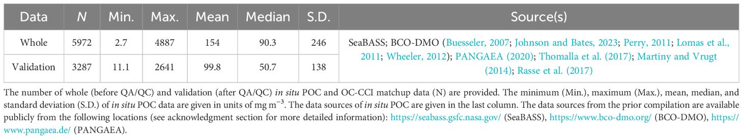
Table 1 Summary of the in situ POC data matched with the OC-CCI products (1997-2020).
2.2 Satellite data
Daily OC-CCI version 5 products (Sathyendranath et al., 2021) at 4 km resolution were used for algorithm validation, and monthly composites for indirect validation and for POC time-series product generation (1997–2020). The OC-CCI products were generated based on MERIS (MEdium-Resolution-Imaging-Spectrometer) as the reference sensor. Remote sensing reflectance (Rrs) at multiple wavelengths (λ at 443, 490, 510, 560, and 665 nm), chlorophyll-a biomass (B), and backscattering coefficient (bbp) at 490 nm were extracted from the OC-CCI products according to algorithm requirements. As some POC algorithms were initially developed for different sensors and their spectral bands, the Rrs(λ) retrieved from the OC-CCI products were shifted in reverse to obtain those wavebands (e.g., Rrs(555)) using the same band-shifting approach that was used when generating the OC-CCI data (Mélin and Sclep, 2015; Jackson et al., 2017; Sathyendranath et al., 2019). The memberships of each optical water class (1–14) (Jackson et al., 2017) were also extracted from the OC-CCI for uncertainty estimation, for mapping per-pixel uncertainties, and for estimating dominant optical water classes.
2.3 In situ POC and satellite matchup data
In situ POC data were matched with the OC-CCI products, following the approach of Evers-King et al. (2017) and Jackson et al. (2017). Prior to the matchup process, the in situ POC data from the same location and date were averaged over the top 10 m, and over the day of sampling. The satellite pixel containing the same location and date as the in situ POC observation was treated as the central pixel for data extraction. When the central pixel was valid, a window of 3 by 3 pixels around the central pixel were also extracted, and their mean, median, and standard deviation were computed for all relevant variables retrieved from the OC-CCI data. The number of valid pixels in the window of 3 by 3 pixels was also noted. The total number of matchup data between the in situ POC and OC-CCI data was 5972 (Table 1, whole matchup data). These data were then subjected to quality control and assessment. Only the subset of data (Table 1, validation matchup data) that passed the control and assessment was then used for further analyses, including algorithms validation.
The geographical locations where the in situ POC measurements were taken and successfully matched with the OC-CCI products cover a wide range of oceanic environments, including coastal and open oceans (Figure 1). The histogram of the in situ POC data showed a bimodal positively-skewed distribution pattern with median and mean of 90.3 and 154 mg m−3, respectively (Figure 2A, blue). The highest peak is associated with a large number of data collected in oligotrophic gyres during the Atlantic Meridional Transect cruises (Rasse et al., 2017; Evers-King et al., 2017). The second peak is associated with data collected from the coastal waters of eastern and western North America.
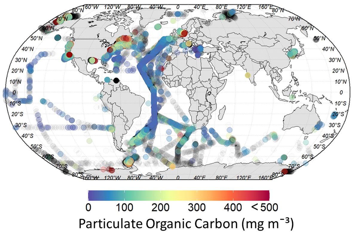
Figure 1 Geographical distribution of in situ POC data (0–10 m) that matched with valid satellite data for September 1997 to January 2020 (Table 1, whole matchup data). The colour of circles indicate the POC concentration (mg m−3) of in situ data. Grey circles indicate the locations of unmatched data point that were excluded in the analysis.
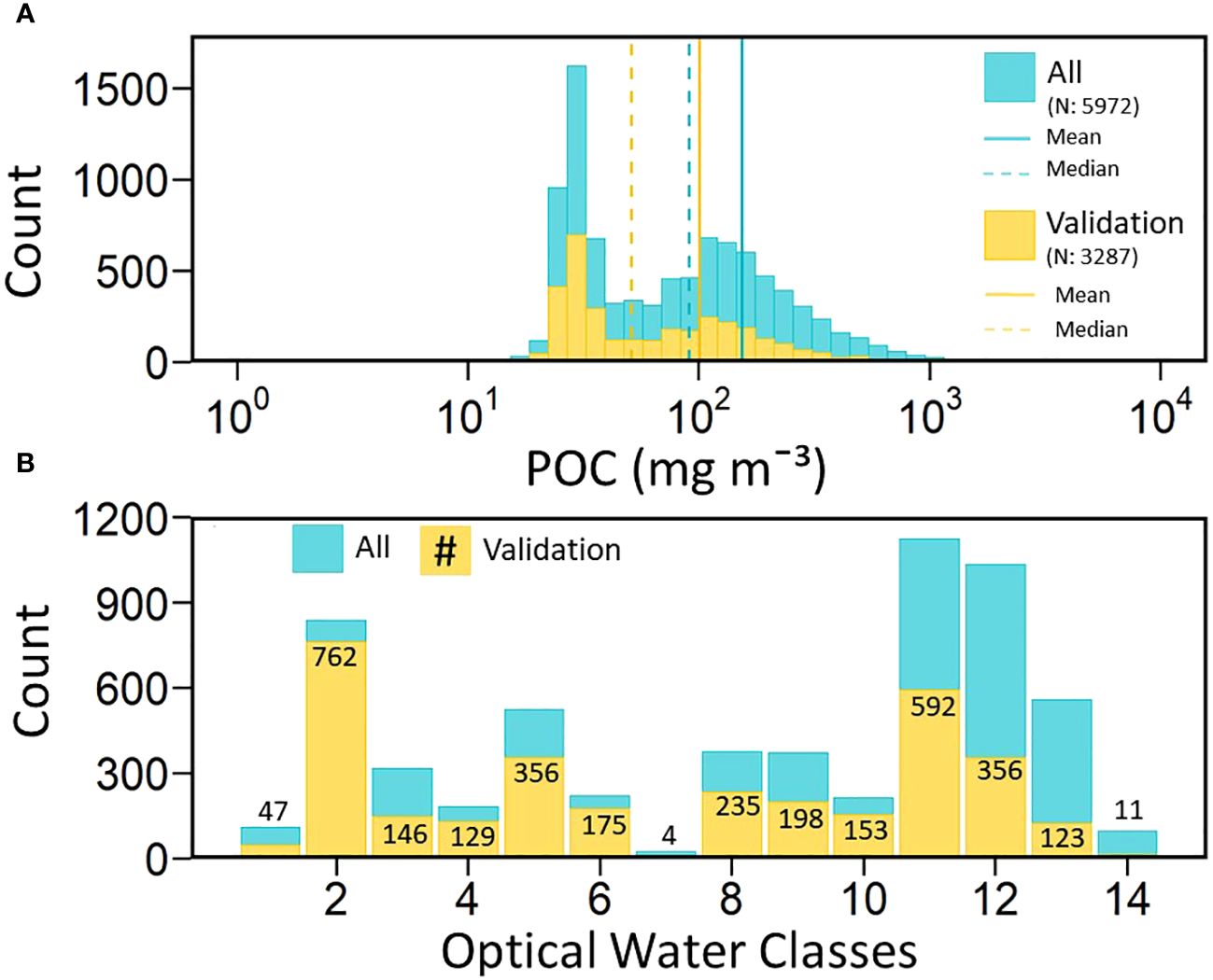
Figure 2 (A) Histograms of the in situ POC (mg m−3) values for the whole (blue) and validation (yellow) matchup data (1997–2020). The in situ POC and OC-CCI matchup data that were retained after quality control and assessment constitute the validation data set (see section 2.5). The dashed and solid lines represent the median and mean values for the whole (blue) and the validation (yellow) matchup data, respectively. (B) Frequency distributions of the matchup data per dominant water class (1–14) derived from the OC-CCI products, for the whole (blue) and the validation (yellow) matchup data. The numbers represent the number of validation matchup data per dominant water class. Note that only the validation data set is used in the rest of the work.
2.4 Mixed-layer depth
A global, monthly climatology of mixed-layer depth from de Boyer Montegut et al. (2004) was used to estimate the total standing pool of POC in the mixed layer (http://dx.doi:10.1029/2004JC002378).
2.5 Quality control and assessment
Several quality control criteria were applied to the data sets (Table 1, whole matchup data) for removing potentially erroneous in situ POC and OC-CCI matchup data. First, all matchup data points pertaining to inland waters were removed. Second, about 2.4% (N = 147) of matchup data that contained less than four valid pixels in the 3 by 3 pixel-box around the central pixel were excluded as adjacency to invalid pixels might indicate potential pixel contamination. Third, a group of some 24 in situ POC observations collected from a small geographical area, and close together in time, appeared as outliers when the in situ POC data were plotted against corresponding chlorophyll-a data. These stations, with POC concentration less than 10 mg m−3 and chlorophyll-a concentration greater than 0.06 mg m−3 (N = 24), were removed as being potentially erroneous. In addition, a data point with a very high POC concentration (> 4000 mg m−3) was removed. Lastly, OC-CCI variables for which the coefficient of variation (standard deviation divided by the mean) exceeding 0.15 for the valid pixels in the 3 by 3 pixel-box (see Appendix A) were also removed. The high spatial variability surrounding the central pixel could be indicative of locations where uncertainties could be high because of mismatches in time and space between in situ POC and satellite observations. The quality control procedure is designed to ensure that the matchup data used in validation and analysis are of high quality, and to eliminate any data with significant bias (Bailey and Werdell, 2006).
After the quality control procedures, 3287 samples, or about 55% of the initial in situ POC data matched with the OC-CCI products were retained for use in validation and related analyses (Table 1, validation data). The remaining matchup data of questionable quality were not used in the rest of this work. Though many matchup data were lost during this procedure, with a high proportion of data lost in optically complex waters (Figure 2B, water classes 11–14), the histogram of the validation matchup data (Figure 2A, yellow) show a distribution pattern similar to that of the initial matchup data (Figure 2A, blue), with median and mean of 50.7 and 99.8 mg m−3, respectively. The size of the validation matchup data set of over three thousand observations is one to two orders of magnitude higher than that of the data sets used for the development of the candidate algorithms (see section 2.6). This implies that advantages that any of the algorithms might have, because of the overlap between the data used for development and validation, is likely to be low. The validation matchup data may, however, still contain some potentially low-quality in situ POC and satellite-derived products due to a variety of factors, including differences in data collection methods, calibration procedures, and instruments.
2.5.1 Per-pixel uncertainty estimates and optical water classes
Each validation matchup data point (Table 1) was assigned to a dominant optical water class (1–14) associated with its central pixel, estimated from the water class membership values retrieved from the OC-CCI products (Jackson et al., 2017). In general, the lower water classes (1–2) correspond to oligotrophic waters with maximum Rrs at the short wavelengths of the visible spectrum, whereas the high water classes (13–14) correspond to turbid waters with relatively higher Rrs at longer wavelengths (see Appendix B). The total number of validation matchup data varied across the dominant optical water classes, with water class 2 showing the largest number (N = 762) of data points, followed by water classes 11 and 12 (Figure 2B, yellow). On the other hand, water classes 7 and 14 show very low number of the data points (N = 4 and 11, respectively). The segregation of the validation matchup data into dominant optical water classes served two major purposes: (i) it allowed us to evaluate whether the algorithm performance was linked to the optical complexity of the water represented by the optical class, especially as not all algorithms were originally intended to be used indiscriminately across all types of waters; and (ii) to estimate uncertainties for each water type, which could then be used to map uncertainties on a per-pixel basis (Jackson et al., 2017; Evers-King et al., 2017; Sathyendranath et al., 2019).
2.6 Candidate POC algorithms
Since the first development of an ocean-colour-satellite-based POC algorithm in the late 1990s (Stramski et al., 1999), various algorithms have been proposed to estimate POC concentration from satellite observations in coastal and oceanic waters. These can be categorised into algorithms that use Rrs band ratios (Stramski et al., 2008), or a combination of maximum Rrs band ratio and band ratio difference index (Stramski et al., 2022), or backscattering and chlorophyll-a (Loisel et al., 2002), or the colour-index (Le et al., 2018). These algorithms were formulated using different types of in situ and satellite data sets. For example, while the colour-index algorithm (Le et al., 2018) was formulated using satellite-derived Rrs matched with the in situ measurements of POC, the other algorithms were formulated using only in situ observations. Of these, seven candidate algorithms were selected to be representative of distinct algorithmic types in the analyses presented here, and they are described below in sections 2.6.1–2.6.4. It is important to note that in this paper the validation is carried out over the global ocean, regardless of whether the algorithms were originally intended to be used so broadly. For consistency, all algorithms were evaluated using input variables derived from the same set of satellite products (OC-CCI; version 5) and the same validation data set (Figure 2, yellow).
2.6.1 Band ratio algorithms: S1, S2, S3, and S4
Stramski et al. (2008) developed empirical POC algorithms based on the blue-green band ratio of Rrs(λ). The band ratio empirical algorithms were developed using in situ measurements of Rrs matched with in situ POC collected from the oligotrophic and upwelling waters of the eastern South Pacific and Atlantic Oceans. In the 53 data points used for the algorithm development, POC ranged from 10–270 mg m−3 (Stramski et al., 2008). The band ratio algorithm that uses Rrs(443) and Rrs(555) (see Equation 1 below) is currently adopted by NASA to generate their standard POC products. While the NASA has adopted the band ratio algorithm to generate global POC products, these algorithms are originally intended to be used for open oceans, where POC is less than 300 mg m−3. Similar band ratio algorithms have been also developed for the Southern Ocean (Allison et al., 2010) and South China Sea (Hu et al., 2016), to improve performance in those regions. Here, we have selected the following four band ratio algorithms (S1–S4; Equations 1–4) from Stramski et al. (2008) that performed well in an earlier evaluation (Evers-King et al., 2017).
Here, represents satellite-derived POC.
2.6.2 Hybrid algorithm: ST
Stramski et al. (2022) developed ocean color sensor-specific hybrid algorithms based on mechanistic principles to improve satellite-derived POC products across a continuum of water bodies with varying optical properties and particle composition. The hybrid algorithm was developed using field data sets collected in various water types, with POC ranging 11.9–1022 mg m−3 (Stramski et al., 2022). The algorithm uses a blending of maximum band ratio and band ratio difference index: the band ratio difference index component is used for POC less than 15 mg m−3, the maximum band ratio algorithm is used for POC greater than 25 mg m−3, and the weighting approach of these two components is applied for the region of transition (Stramski et al., 2022). In the implementation here, we used the hybrid algorithm (hereafter, labelled ST) developed for the MERIS sensor, since the OC-CCI version 5 products are reported for MERIS wavebands.
2.6.3 Particle backscattering and chlorophyll-a based algorithm: LO
Loisel et al. (2002) developed a semi-analytical algorithm based on the assumption that the particle backscattering (bbp) covaries with POC concentration for oceanic waters (Equation 5). This algorithm (labelled LO here) exploits the relationship between bbp/bp (where bp is the particle scattering coefficient) and B developed by Twardowski et al. (2001), which allows the slope of bbp versus POC to vary with tropic status. To take this into account, a fixed mean POC/bp value of 400 is used in the algorithm (Loisel et al., 2002), leading to the following relationship.
The algorithm LO (Equation 5) was initially implemented on POLDER (Polarization-and-Directionality-of-the-Earth’s-Reflectances) and SeaWiFS (Sea-viewing-Wide-Field-of-View-Sensor) satellite data. This algorithm was validated using a set of matchup data collected from the North Pacific Subtropical gyres (N = 24) and North Atlantic Central gyre (N = 30) (Loisel et al., 2002). This algorithm performed relatively well in the analyses of Evers-King et al. (2017) that used the in situ POC and OC-CCI matchup data. In the implementation here, we used the chlorophyll-a data from the OC-CCI. The bbp at 490 nm was estimated using the algorithm of Loisel et al. (2018), rather than using the bbp data from the OC-CCI, for algorithm consistency.
2.6.4 Colour-index algorithm: LE
Le et al. (2018) developed a POC algorithm based on differences in two pairs of Rrs values, known as the colour-index. In contrast to other approaches, this algorithm was developed using satellite-derived Rrs and in situ POC data. The colour-index algorithm was tested for three satellite sensors: SeaWiFS, MERIS, and MODIS (Moderate-Resolution-Imaging-Spectroradiometer). As for the other algorithms, we chose the MERIS algorithm here (Equations 6, 7):
where D stands for the colour-index. The D is then used to estimate the concentration of POC using algorithm LE:
2.7 Statistical metrics
Statistical metrics recommended by the algorithm developers and those in general use in the ocean-colour community (Brewin et al., 2015; Evers-King et al., 2017; Seegers et al., 2018; Stramski et al., 2022; Joshi et al., 2023) were used to assess the performance of candidate algorithms. The statistic metrics were applied between the in situ POC and satellite-derived POC matchup data (N = 3287): the root-mean-square difference (φ), centred-pattern-root-mean-square difference (Δ), and bias (ψ) for both log-transformed and non-transformed POC matchup data (see Appendix C for the equations used). The Pearson’s parametric correlation coefficient (r) was calculated for log-transformed data, and Spearman’s correlation coefficient (rs) was calculated for non-transformed data. The median ratios (δ) and median absolute percentage difference (τ) were estimated for non-transformed data. The median symmetric accuracy (κ) was estimated for log-transformed data. Compared with the other statistics, the κ does not penalize both over-and under-prediction differently (Joshi et al., 2023). The slope (S) and intercept (I) of the linear fit between in situ POC and satellite-derived POC matchup data were estimated from the standard major axis of model type II linear regression (Ricker, 1973; Sokal and Rohlf, 1995). Condorcet’s pair-wise comparisons of residuals (Seegers et al., 2018; Stramski et al., 2022) were performed for log-transformed and non-transformed data as an additional test.
3 Results
3.1 Performance of the candidate algorithms
The satellite-derived POC data were plotted against the in situ POC validation matchup data for each candidate algorithm (S1, S2, S3, S4, ST, LO, and LE) under consideration, along with the fitted linear regression line, for algorithm validation (Figure 3; Table 2). The dominant water classes (1–14) associated with each point are also indicated using colours, to assist assessment of algorithm performance across different optical water classes. It is particularly important to check algorithm performance in those water classes that are poorly represented in the validation matchup data (e.g., water classes 7 and 14). In general, the POC concentration increased with the number of the optical water classes associated with them, as seen from the progression of colours in the scatter plots from blue to red, or from water classes 1 to 14 (Figure 3).
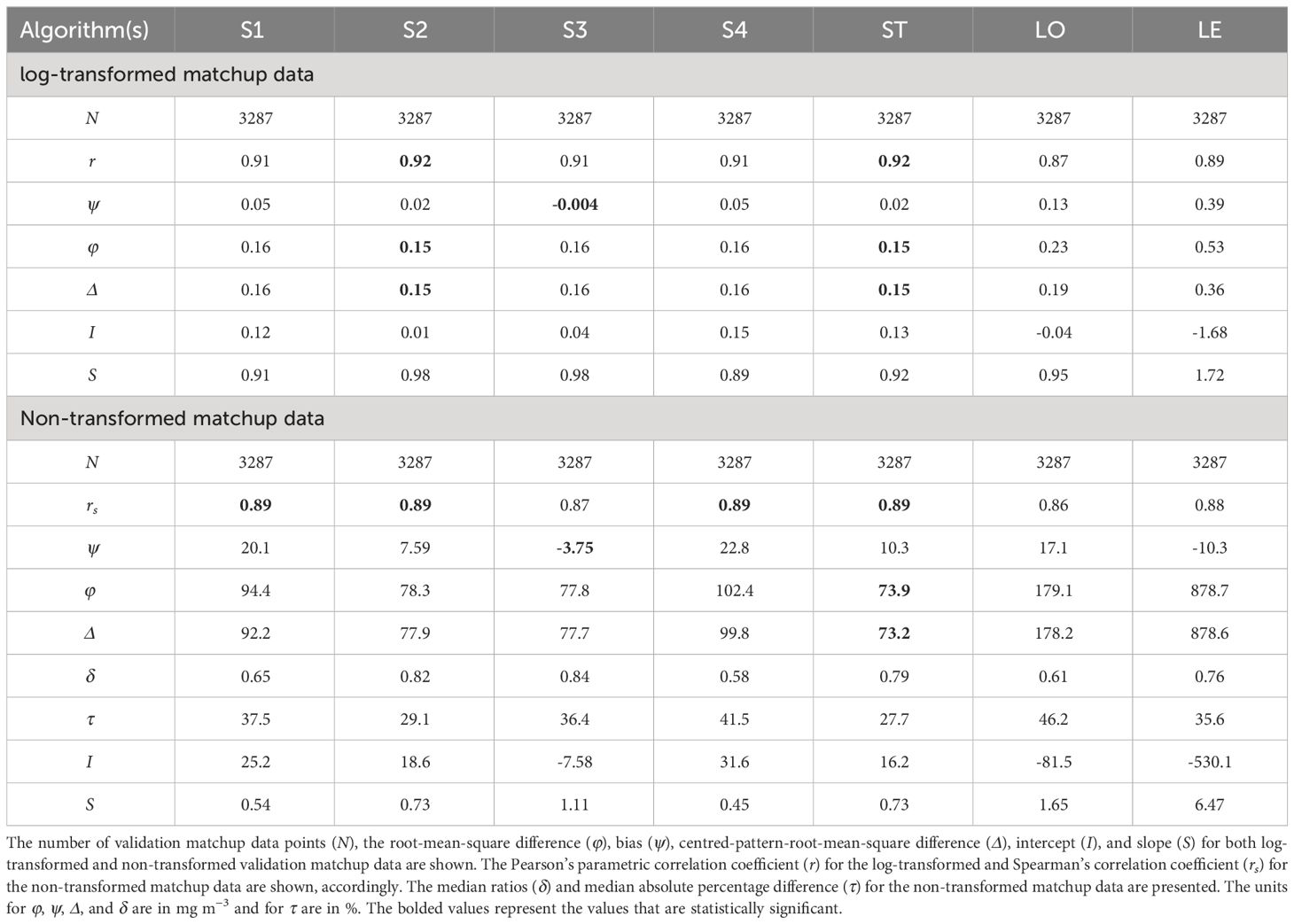
Table 2 Summary of statistical performance of the candidate algorithms.
Overall, algorithms S2, S3, and ST performed well, with high r values (0.91–0.92) for the log-transformed matchup data, and with lower uncertainties than the other algorithms (Figure 3; Table 2). Some differences were observed among band ratio algorithms (S1, S2, S3, and S4), especially in water classes 13–14, where algorithm S4 tended to underestimate POC concentrations. Although the differences between these band ratio algorithms are statistically small, algorithm S2 presented the lowest uncertainties over the whole dynamic range of POC concentration for log-transformed matchup data in this analysis, with the fitted regression lying closest to the 1:1 line (Figure 3C). The performance of algorithm S2 is statistically similar to algorithm ST, but with intercept and slope closer to 0 and 1 respectively, for log-transformed matchup data.
The modified Taylor diagram (Taylor, 2001) (Figure 4), which combines information on four key statistical metrics — the Pearson’s correlation coefficient, the standard deviation, the centred-pattern-root-mean-square difference (unbiased), and the bias — also conveys the same message: algorithms S2, S3, and ST are clustered together and lie close to the in situ observation curve with high correlation coefficient, indicating statistically similar performances, consistent with the results seen in Figure 3. The algorithms S1 and S4 lie close to these algorithms with similar statistical performances for both non-transformed and log-transformed matchup data sets. The algorithm LO also lies close to these algorithms, albeit with higher errors and lower r for non-transformed matchup data (Figure 4A). When divided into dominant water classes, the performance of all candidate algorithms were lower than when examined as whole data sets, especially for water classes 1–10 with r below 0.5 (see Appendices D, E).
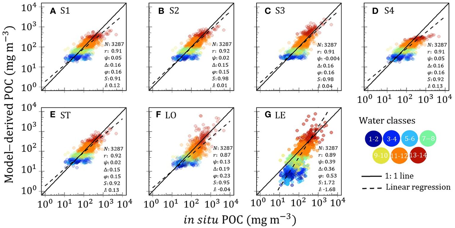
Figure 3 Relationships between in situ POC and corresponding satellite-derived POC matchup data (mg m−3) estimated from candidate algorithms (A) S1, (B) S2, (C) S3, (D) S4, (E) ST, (F) LO, and (G) LE. The solid line is the 1:1 line. The dashed line is the best fit for linear regression. The colour assigned to the data points indicate the corresponding dominant optical water classes (1–14). The number of validation matchup data points (N) is shown. The Pearson’s parametric correlation coefficient (r), root-mean-square difference (φ), centred-pattern-root-mean-square difference (Δ), and bias (ψ), as well as slope (S) and intercept (I) for the linear fit to log-transformed validation matchup data are shown.
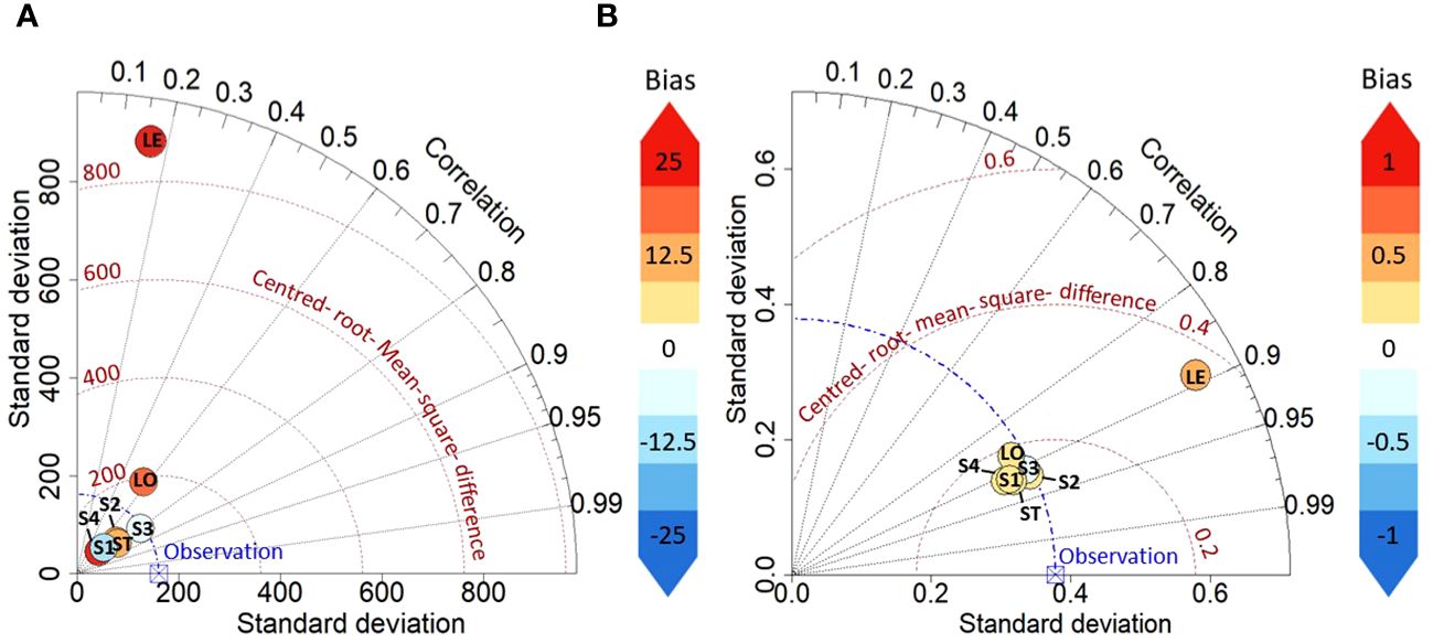
Figure 4 Modified Taylor diagrams comparing the (A) non-transformed and (B) log-transformed satellite-derived POC data estimated from candidate algorithms (S1, S2, S3, S4, ST, LO, and LE) and their relationship to the in situ POC data (blue dotted curve) in terms of the Pearson’s parametric correlation coefficient, standard deviation, and centred-pattern-root-mean-square difference (red dotted curves). The colour bar indicates the bias between the in situ POC (mg m−3) and satellite-derived POC data (mg m−3).
Although the uncertainties associated with algorithm LE were generally relatively high (Figure 4), the spread of data points is most elongated for this algorithm, showing a better separation among the different optical classes (Figure 3). This suggests the algorithm LE has a higher sensitivity, compared with all the other algorithms, especially for low POC concentrations (Figure 3). The main issue with algorithm LE was the deviation of the slope of the regression equation from the 1:1 lime. This could have occurred simply (i) from the differences between the modest set of data that was used initially to develop the algorithms, compared with the data set employed here for testing them; (ii) from implementing the algorithms on different satellite products from the ones used for the development, even though we took care to minimise errors arising from this source; or (iii) from the formulation of the algorithm itself, as it was established with a specific set of satellite-derived Rrs. When we applied a linear transformation to each of the algorithm outputs using the slope and intercept of the fitted linear regression for that algorithm, this had the effect of rotating the adjusted outputs to the 1:1 line when re-plotted against the matchup data (which can no longer be considered validation data at this stage). This adjustment (results not shown) had the most positive impact on algorithm LE, bringing it close to the band ratio algorithms on the Taylor diagram for the adjusted outputs, implying that this algorithm has the potential for further improvement.
3.1.1 Analysis of residuals
A detailed analysis of residuals, the differences between in situ POC and satellite-derived POC data, was conducted to compare the performances of candidate algorithms (Figure 5). All candidate algorithms presented near-normal distributions of residuals, with a peak near zero (result not shown). The band ratio algorithms (S1, S2, S3, and S4), as well as algorithms LO and ST, showed relatively small residuals compared with the other algorithms, but there was a distinct systematic pattern of change in residuals with the water types (Figure 5). Such water-type-dependent residuals might offer possibilities for further reductions in residuals, especially if algorithm development could be carried out independently for each water type. But such developments must await the availability of sufficient numbers of high-quality matchup data in each water class.
For all candidate algorithms, the highest residuals are associated with water classes 13–14 (Figure 5). Algorithm LE, for example, presented a small number of residuals exceeding 10,000 mg m−3 for these classes, which adversely affected its performance. The residuals were further analysed using Condorcet’s pair-wise comparison of residuals (Seegers et al., 2018; Stramski et al., 2022). In this analysis, the residuals of pairs of candidate algorithms were compared, and in each comparison, the algorithm for which the residuals were lower the most number of times is considered as the ‘winner’. The final ‘winner’ is the algorithm with the highest % wins (> 50%) for all pair-wise comparison of residuals. According to this test, algorithm S3 performed the best, followed by algorithms ST, LO, and then S2 for non-transformed data (Figure 6A), consistent with the results shown in Figure 3. For the log-transformed data, the algorithm ST was the ‘winner’, but the % win was relatively low except when compared against algorithm LE (Figure 6B).
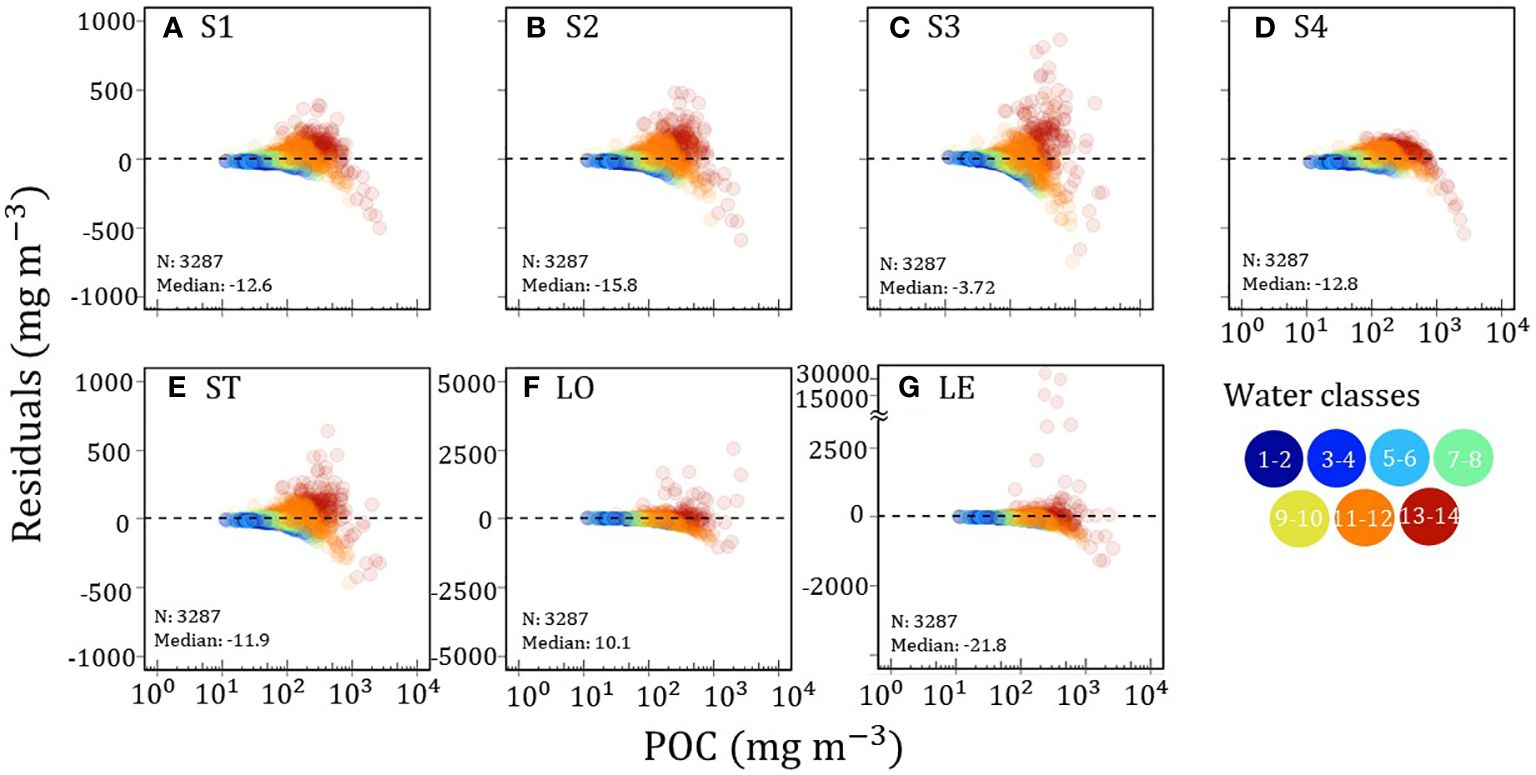
Figure 5 Scatter-plots of residuals, computed as the difference between in situ POC and satellite-derived POC for candidate algorithms (A) S1, (B) S2, (C) S3, (D) S4, (E) ST, (F) LO, and (G) LE, are plotted as a function of in situ POC. The colours of the data points indicate the associated dominant water types (1–14) estimated from the OC-CCI products. The dashed line indicates where the residual equals to zero. The units for residuals and in situ POC are in mg m−3.
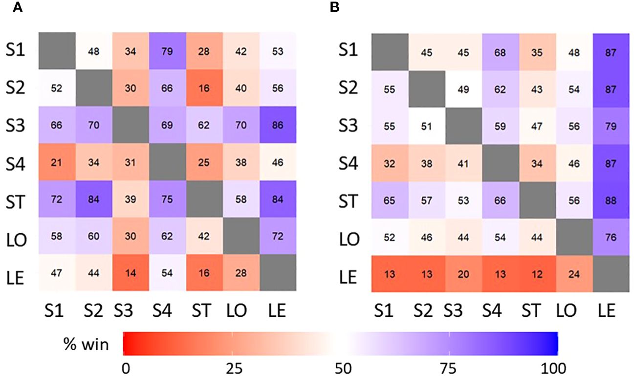
Figure 6 Condorcet’s pair-wise comparison of residuals between a pair of candidate algorithms (S1, S2, S3, S4, ST, LO, and LE) for (A) non-transformed and (B) log-transformed POC data. Blue colour represents instances when residuals of an algorithm win over another algorithm. The % win is shown in both colours and numbers. White and red colours represent when the residuals of an algorithm tie or lose against another algorithm, respectively. The magnitude of the wins (>50%) and losses (<50%) are indicated by the intensity of the blue and red colours, respectively. The number of total wins or losses is counted horizontally.
3.2 Relationship between POC and chlorophyll-a biomass
Comparison of satellite-derived products against in situ observations is an essential step in the validation of algorithms, but it is not necessarily a sufficient step. Paucity of matchup data; mismatches in the times of observations (though the matchup criteria are designed to minimise such errors); differences in spatial scales of satellite and in situ observations; lack of representative samples from all relevant regions and seasons — all these introduce uncertainties into such validation exercises. Therefore, as a complement to matchup comparisons, we have attempted here an indirect validation by comparing the patterns in the relationship between POC and chlorophyll-a concentration. We examine whether the relationship observed when in situ POC is plotted against satellite-derived chlorophyll-a is reproduced when satellite-derived POC is plotted against corresponding chlorophyll-a concentration, as in Evers-King et al. (2017).
In the left panel of Figure 7, the satellite-derived POC is plotted against the corresponding matchup satellite-derived chlorophyll-a. Since the relationship appears to be piece-wise linear with discontinuities at 0.1 and 1 mg m−3, linear regressions were fitted to the data for chlorophyll-a concentration ≤ 0.1 mg m−3 (range 1), 1 mg m−3 (range 2), and chlorophyll-a ≥ 1 mg m−3 (range 3). The in situ POC is also shown as a background in grey in all the panels. Ideally, in this comparison, we are looking for algorithms that reproduce the fits and the spread of data around the fits that are observed for the in situ matchup data, for all the three chlorophyll-a ranges. The in situ POC (grey colour in Figure 7) was poorly correlated with chlorophyll-a in range 1, but the correlation was stronger in ranges 2 and 3. The algorithms S1, S2, S3, S4, ST, and LO (Figure 7) followed a similar pattern to that of the in situ relationship. Algorithms LE (Figure 7) showed stronger deviations from the in situ relationships, especially for water classes 1 to 10 (range 1 and range 2 of chlorophyll-a concentration).
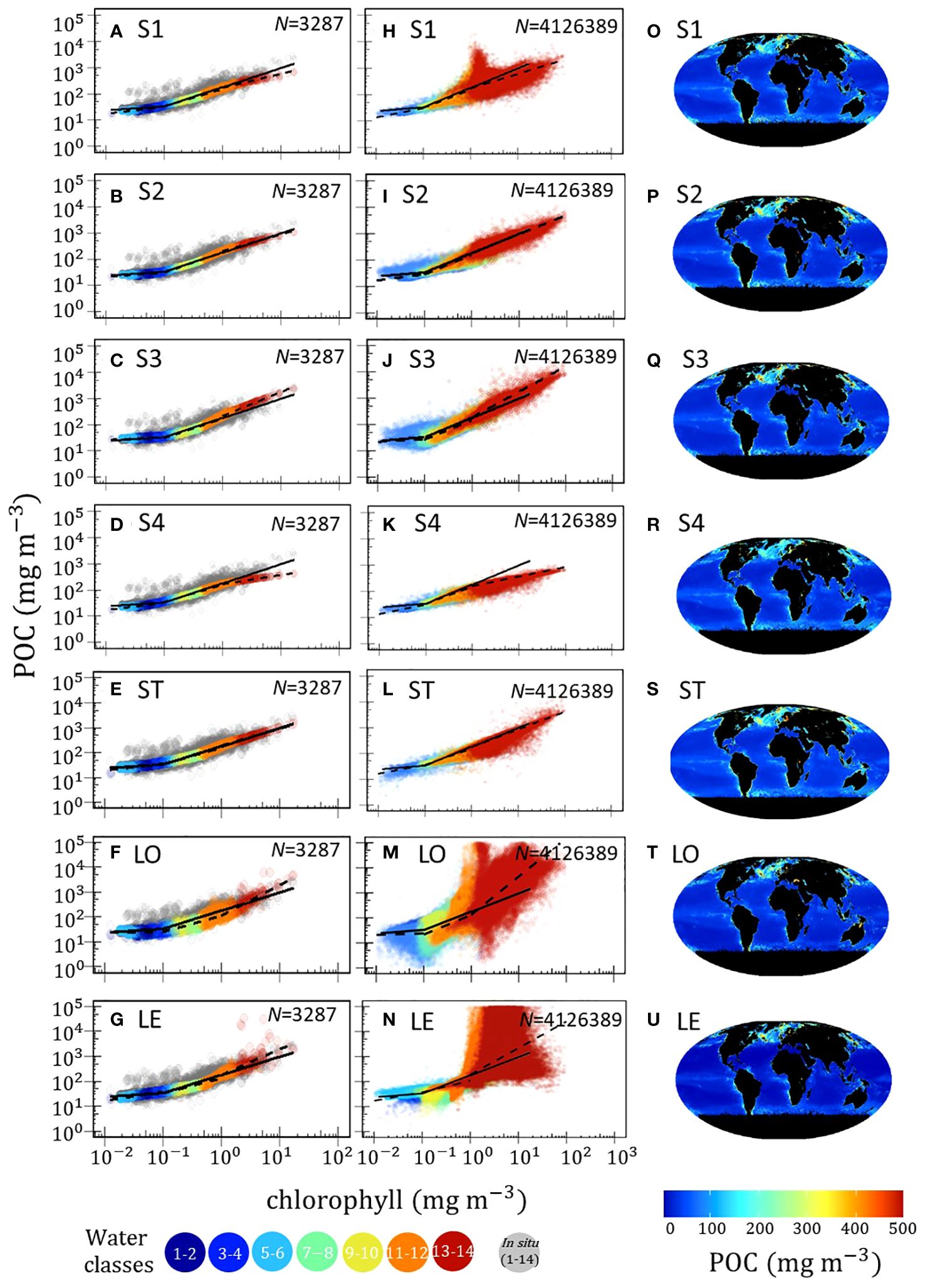
Figure 7 Satellite-derived POC estimated from candidate algorithms (S1, S2, S3, S4, ST, LO, and LE) compared with corresponding satellite-derived chlorophyll-a data. The (i) POC and chlorophyll-a relationships from the validation matchup data [left panels, (A–G), (ii) the POC and chlorophyll-a from a sample monthly composite OC-CCI image (June, 2020) (middle panels, (H–N)], and (iii) the spatial maps of the POC estimated from the same monthly composite OC-CCI images (right panels, (O–U). The solid lines in the scatter plots (i) and (ii) represent the linear regressions estimated from the in situ POC and satellite-derived chlorophyll-a matchup data for three different chlorophyll-a ranges: chlorophyll-a less than or equal to 0.1 mg m−3 (range 1), between 0.1 and 1 mg m−3 (range 2), and equal to or greater than 1 mg m−3 (range 3) (see Appendix F). The dashed lines represent the corresponding linear regressions estimated for the satellite-derived POC and the same satellite-derived chlorophyll-a values.
We also plotted the satellite-derived POC data against the satellite-derived chlorophyll-a for all valid pixels for a randomly selected monthly OC-CCI image (June 2020) (Figures 7H–N), to see whether the satellite-derived POC and chlorophyll-a relationships resembled that of matchup data Figures 7A–G). The regression equations are fitted for the same three ranges of chlorophyll-a, as in the left panel. The regression line of in situ POC and chlorophyll-a estimated for the validation matchup data (solid line in left panel of Figure 7) is also reproduced in the middle panel as a common reference line. The number of valid satellite pixels obtained from the monthly image of 9 km resolution was 4,126,389.
In the comparison for the global data (middle panels, (Figures 7H–N), algorithms S1, S2, S3, S4, ST, and LO presented satellite-derived POC and chlorophyll-a relationships that are fairly similar to the matchup results on the left. However, the middle panels revealed some differences among these four algorithms that were not so evident when only the matchup data were plotted in the left panels. For example, the spread of the data points in the vicinity of 1 mg m−3, is high for algorithm S1, whereas such a feature is not seen in the left panel of Figure 7A, and may be related to increased noise in the Rrs values at 443nm, as chlorophyll-a concentration increases, and when satellite viewing angles are unfavourable: we found that most of these data points were located in high-latitude waters (40 °S and above) during the southern hemisphere winter (data not shown). It is also seen that the scatter of points in range 1 is less for algorithms S1 and S4 than for algorithms S2 and S3.
To investigate the performance of candidate algorithms in high-latitude waters from where we lack sufficient in situ POC and satellite-derived matchup products for point-by-point comparison, we examined the monthly sea-surface POC concentration in sub-Antarctic waters derived from algorithms ST and S2 (two of the algorithms that performed well in the comparisons) with the POC data derived from BGC-Argo (see Appendix G). The comparison mirrors that carried out by Galí et al. (2022), and is carried out for the Sub-Antarctic region, as defined by them. In Galí et al. (2022), POC was estimated using mixed layer depth and bbp(700) obtained from a monthly climatology from BGC-Argo data (2014-2019). For comparison, we combined monthly POC concentrations (1998-2020) derived from ST and S2 algorithms at each location with mixed-layer depth data (section 2.4) to estimate the POC pool in the layer. Both algorithms, ST and S2, showed values similar to BGC-Argo POC data from April to October. However, the winter average for the area (months 1 and 12 in the figure) overestimates BGC-Argo-based estimates and the model-based estimates of Galí et al. by a factor of two to three, which could reflect the poor sampling of high-latitudes by satellites during the winter months, such that the satellite-based estimates are biased towards the higher POC values at lower (less southern) latitudes. While it is difficult to carry the comparison further, it provides some reassurance that the satellite-derived estimates are not unreasonable in regions from where there are no to little matchup data.
4 Discussion
In this paper, we have compared a number of algorithms that have been proposed for estimating POC from satellite data with the objective of finding the best performing algorithm when used in conjunction with the OC-CCI time series data, for global applications, especially in the context of studying the impact of climate change on the marine environment. In doing this, we have, in some instances, taken some algorithms beyond the specific purposes for which they were designed. For example, some of the algorithms were designed for specific localities. If such algorithms that were tuned for excellence in a particular environment under-performed in the global context, it may not be totally surprising, and it should not be taken as indicative of their value and usefulness when they are used for the application for which they were originally designed. Nevertheless, such comparisons could provide new insights into how the various types of algorithms might be improved further, and where future efforts might be targeted.
Given the objective of applying the algorithm to the OC-CCI version 5 products, which were developed with MERIS as the reference sensor and with Rrs values reported for the MERIS wavebands in the visible domain (412, 443, 490, 510, 560, and 670nm), Rrs values from the OC-CCI products had to be shifted to the bands used in the initial implementation of the algorithms, which could have added to the differences between algorithms and in situ matchup data. In spite of all such problems which made the algorithm-data comparisons difficult, it was algorithms S2 and ST that performed consistently well, though several other algorithms performed almost as well.
POC estimates computed using algorithm S2 have been implemented with OC-CCI data version 4.2, based on its performance in an earlier comparison (Evers-King et al., 2017) and also because of its excellent performance in the comparisons presented here (the data are openly available here (Sathyendranath et al., 2022a): https://catalogue.ceda.ac.uk/uuid/299b1bb28eaa440f9a36e9786adfe398). The global average over the entire time series of POC concentration (1998-2020) estimated from algorithm S2 was 1.07 ± 0.05 PgC (where the uncertainty is the standard deviation associated with the year-to-year differences). This is similar to estimates from the past inter-comparison study (Evers-King et al., 2017), which lay in the range from 0.77 to 1.3 PgC. Since the original algorithm S2 was developed with a small number of matchup data (of order 100), and also because of the differences in wavebands used for algorithm development and those available on the OC-CCI version 5 products, we used the extensive matchup data sets consisting of in situ POC and satellite products assembled here to re-tune the algorithms to the OC-CCI data, before implementation (see Appendix H). The excellent performance of the tuned algorithm, with the low uncertainties associated with the POC product, gives confidence in its quality, especially for those optical classes for which a large number of matchup data were available (the tuned algorithm S2 data are openly available here (Sathyendranath et al., 2022b): http://dx.doi.org/10.5285/5006f2c553cd4f26a6af0af2ee6d7c94). Our results indicate that algorithm ST also merits to be implemented as a global time series.
The optical classes that are poorly represented in the in situ data direct us to areas where future validation exercises should be prioritised. Certainly, the next big challenge is to improve the performance of POC algorithms in coastal waters, for which there is a need for enhancement in the number of observations available from under-represented coastal water classes and from under-represented geographic areas, such as the Indian Ocean and high-latitude waters (Figure 1).
While we consider the needs for a step change in the number of in situ observations, and where they are needed, we should also highlight the importance of high-quality data. Empirical POC algorithms depend heavily on the quality of both the Rrs and in situ POC data. Most of the in situ data assembled in this study were measured following the protocols established during the Joint Global Ocean Flux Study (Knap et al., 1996). Even though the data had been subjected to rigorous quality checking by data providers and by us, some data points with high bias could have gone undetected in the data, which is a compilation of data from various investigators collected from different oceanographic cruises covering a period of over two decades. Residual errors can be difficult to identify, though we were able to spot a small number of outliers on the basis of a comparison with corresponding chlorophyll-a data. The comparison allowed us to identify data with unrealistic carbon-to-chlorophyll ratios. Additional uncertainties are introduced at the matchup step, when discrepancies can stem from differences in temporal and spatial scales of in situ and satellite observations. We employed rigorous satellite-matchup criteria to minimise errors from this source. The downside was that it removed over 2000 matchup data points. While the quality control added confidence in the results, it also pointed to the need for consistency in methodology and data management to ensure the high quality of in situ POC data. In addition, improvements to methodologies used for in situ data collection are also needed, as the works of Novak et al. (2018) and Stramski et al. (2022) indicate.
Given the limitations of direct validation of satellite algorithms, we explored indirect modes of testing the products, by comparing relationships between POC and chlorophyll, similar in approach to that of Evers-King et al. (2017) and by comparing regional estimates of POC in the sub-Antarctic region. These comparisons were helpful in identifying problems not only with the algorithms per se, but also in highlighting instances when an increase in uncertainties in satellite products under unfavourable viewing conditions could translate into enhanced errors in the POC product. Whereas such errors are not a limitation of the algorithm itself, it illustrates conditions when such algorithms may not be applicable. They also point to instances where consistent gaps in satellite data (such as in high latitudes) could limit interpretation of data aggregated at large scales.
5 Concluding remarks
The results presented here confirm earlier conclusions that POC algorithms have reached a state of maturity where they meet user requirements (Evers-King et al., 2017). But one could envisage further developments to algorithm performance by blending multiple POC algorithms according to the performance of each algorithm in different optical water types, as is being done in the OC-CCI chlorophyll-a product (Jackson et al., 2017); or as demonstrated by the hybrid algorithm of Stramski et al. (2022). However, we lack sufficient matchup data from many optical water types, especially water classes 1, 7, and 14 (Figure 2B), and development of water-type-based blended algorithms must await a significant increase in matchup data, especially in these optical classes.
Data availability statement
The data sets presented in this study can be found in online repositories. The names of the repository/repositories and accession number(s) can be found below: https://www.bicep-project.org/Deliverables.
Author contributions
CK: Writing – original draft, Writing – review & editing. SS: Writing – original draft, Writing – review & editing. TJ: Data curation, Writing – review & editing. RB: Writing – review & editing. GK: Writing – review & editing. BJ: Data curation, Writing – review & editing. DS: Writing – review & editing. HL: Writing – review & editing. MG: Writing – review & editing. CL: Writing – review & editing.
Funding
The author(s) declare financial support was received for the research, authorship, and/or publication of this article. This work has been carried out as part of the European Space Agency’s Biological Pump and Carbon Exchange Processes (BICEP) project and by the Simons Collaboration on Computational Biogeochemical Modeling of Marine Ecosystems (CBIOMES) (549947 SS). The work has been also supported by the National Centre for Earth Observations (NCEO) of the UK. MG has received financial support through the OPERA project (PID2019-107952GA-I00).
Acknowledgments
We would like to thank all BICEP project participants for providing feedback on this work, especially Rio, M. and Concha, J. A. for their support. We would like to give special thanks to Jorge, D. who provided great support in processing the satellite data for algorithm LO. Special thanks also goes to Aumont, O. for guiding us on how to use the Sub-Antartic data sets and Röttgers, R. for providing essential feedback on the references. Furthermore, we would like to thank all the scientists who measured and collected the in situ POC data for this study. This includes, but is not limited to (i) SeaBASS: Balch, W., Larouche, P., Stramska, M., Hooker, S., Chaves, J., Mannino, A., Mulholland, M., Reynolds, R., Arrigo, K., Dijken, G., McClain, C., Neeley, A., Camill, P., Roesler, C., Lichter, J., Freeman, S., Novak, M, etc.; (ii) BCO-DMO: Johnson, R. J., Bates, N., Buesseler, K. O., Perry, M., Lomas, M. W., Dyhrman, S. T., Ammerman, J., Wheeler, P., etc; (iii) PANGAEA: Arístegui Ruiz, J., Doblin, M., Bayrakarov, E., etc; (b) (v) other publications: Martiny, A., Vrugt, J., Rasse, R., Dall’Olmo, G., Graff, J., Westberry, T. K., van Dongen-Vogels, V., Behrenfeld, M. J., Thomalla, S. J., Ogunkoya, A. G., Vichi, M., and Swart, S. Without their dedication, this work would not have been possible. In addition, we would like to thank Evers-King, H. and Dall’Olmo, G. for compiling in situ POC data. We would like to express our appreciation to the OC-CCI team for providing satellite products and the National Centre for Earth Observations for funding this study. We sincerely appreciate the valuable feedback and insights of the two reviewers, and we extend our gratitude to our editor, Olson, D. B., for his generous support.
Conflict of interest
The authors declare that the research was conducted in the absence of any commercial or financial relationships that could be construed as a potential conflict of interest.
Publisher’s note
All claims expressed in this article are solely those of the authors and do not necessarily represent those of their affiliated organizations, or those of the publisher, the editors and the reviewers. Any product that may be evaluated in this article, or claim that may be made by its manufacturer, is not guaranteed or endorsed by the publisher.
Supplementary material
The Supplementary Material for this article can be found online at: https://www.frontiersin.org/articles/10.3389/fmars.2024.1309050/full#supplementary-material
References
Allison D. B., Stramski D., Mitchell B. G. (2010). Empirical ocean color algorithms for estimating particulate organic carbon in the Southern Ocean. J. Geophys. Res. 115, C10044. doi: 10.1029/2009JC006040
Bailey S. W., Werdell P. J. (2006). A multi-sensor approach for the onorbit validation of ocean color satellite data products. Remote Sens. Environ. 102, 12–23. doi: 10.1016/j.rse.2006.01.015
Brewin R. J. W., Sathyendranath S., Müller D., Brockmann C., Deschamps P. Y., Devred E., et al. (2015). The Ocean Colour Climate Change Initiative: III. A round-robin comparison on in-water bio-optical algorithms. Remote Sens. Environ. 162, 271–294. doi: 10.1016/j.rse.2013.09.016
Brewin R. J. W., Sathyendranath S., Platt T., Bouman H., Ciavatta S., Dall’Olmo D., et al. (2021). Sinking fux of particulate organic matter in the oceans: Sensitivity to particle characteristics. Earth-Science Rev. 217, 103604. doi: 10.1016/j.earscirev.2021.103604
Buesseler K. O. (2007). Combined water sample data from variety of sampling devices from USCGC Polar Star cruise PS02-2002 in the Southern Ocean, south of New Zealand in 2002 (SOFeX project). Biol. Chem. Oceanography Data Manage. Office (BCO-DMO). doi: lod.bco-dmo.org/id/dataset/2804
CEOS (2014). CEOS strategy for carbon observations from space. The Committee on Earth Observation Satellites (CEOS) response to the Group on Earth Observations (GEO) carbon strategy (Tokyo, Japan: JAXA and I & A Corporation).
de Boyer Montégut C., Madec G., Fischer A. S., Lazar A., ludicone D. (2004). Mixed layer depth over the global ocean: An examination of profile data and a profile‐based climatology. J. Geophys. Res.: Oceans 109 (C12). doi: 10.1029/2004jc002378
Eppley R. W., Peterson B. J. (1979). Particulate organic matter flux and planktonic new production in the deep ocean. Nature 282, 667–680. doi: 10.1038/282677a0
Evers-King H., Martinez-Vicente V., Brewin R. J. W., Dall’Olmo G., Hickman A. E., Jackson T., et al. (2017). Validation and inter-comparison of ocean color algorithms for estimating particulate organic carbon in the oceans. Front. Mar. Sci. 4, 251. doi: 10.3389/fmars.2017.00251
Falkowski P. G., Barber R. T., Smetacek V. (1998). Biogeochemical controls and feedbacks on ocean primary production. Science 28, 200–206. doi: 10.1126/science.281.5374.200
Galí M., Falls M., Claustre H., Aumont O., Bernardello R. (2022). Bridging the gaps between particulate backscattering measurements and modeled particulate organic carbon in the ocean. Biogeosci. 19, 1245–1275. doi: 10.5194/bg-19-1245-2022
Hu S. B., Cao W. X., Wang G. F., Xu Z. T., Lin J. F., Zhao W. J., et al. (2016). Comparison of MERIS, MODIS, SeaWiFS-derived particulate organic carbon, and in situ measurements in the South China Sea. Int. J. Remote Sens 37, 1585–1600. doi: 10.1080/01431161.2015.1088673
Jackson T., Sathyendranath S., Mélin F. (2017). An improved optical classification scheme for the ocean colour essential climate variable and its applications. Remote Sens. Environ. 203, 152–161. doi: 10.1016/j.rse.2017.03.036
Johnson R. J., Bates N. (2023) Niskin bottle water samples and CTD measurements at water sample depths collected at Bermuda Atlantic Time-Series sites in the Sargasso Sea ongoing from 1988. Available online at: http://lod.bcodmo.org/id/dataset/3782.
Joshi I. D., Stramski D., Reynolds R. A., Robinson D. H. (2023). Performance assessment and validation of ocean color sensor-specific algorithms for estimating the concentration of particulate organic carbon in oceanic surface waters from satellite observations. Remote Sens. Environ. 286, 113417. doi: 10.1016/j.rse.2022.113417
Knap A. H., Michaels A., Close H., Ducklow H., Dickson A. (1996). Protocols for the Joint Global Ocean Flux Study (JGOFS) Core Measurements. JGOFS Rep. 19, 1-170. doi: 10.25607/OBP-1409
Le C., Zhou X., Hu C., Lee Z., Li L., Stramski D. (2018). A Color-Index-Based Empirical Algorithm for Determining Particulate Organic Carbon Concentration in the Ocean From Satellite Observations. J. Geophys. Res.: Oceans 123, 7407–7491. doi: 10.1029/2018JC014014
Loisel H., Nicolas J. M., Deschamps P. Y., Frouin R. (2002). Seasonal and inter-annual variability of particulate organic matter in the global ocean. Geophys. Res. Lett. 29, 491–494. doi: 10.1029/2002GL015948
Loisel H., Stramski D., Dessailly D., Jamet C., Li L., Reynolds R. A. (2018). An Inverse Model for Estimating the Optical Absorption and Backscattering Coefficients of Seawater From Remote-Sensing Reflectance Over a Broad Range of Oceanic and Coastal Marine Environment. J. Geophys. Res.: Oceans 123, 2141–2171. doi: 10.1002/2017JC013632
Lomas M. W., Dyhrman S. T., Ammerman J. (2011). Biogeochemistry Data from R/V Atlantic Explorer X0606, X0705, AE0810 in the Western Sargasso Sea roughly 38-20N and 66-43W from 2006-2008 (ATP3 project) (MA. USA: Biological and Chemical Oceanography Data Management Office (BCO-DMO). Available at: http://lod.bcodmo.org/id/dataset/3354.
Mélin F., Sclep G. (2015). Band shifting for ocean color multi-spectral reflectance data. Optics Express 23, 2262–2279. doi: 10.1364/OE.23.002262
Martiny A., Vrugt J. (2014). Concentrations and ratios of particulate organic carbon, nitrogen, and phosphorus in the global ocean. Sci. Data 1, 140048. doi: 10.1038/sdata.2014.48
Müller D., Krasemann H., Brewin R. J. W., Brockmann C., Deschamps P.-Y., Doerffer R., et al. (2015). The Ocean Colour Climate Change Initiative: I. A methodology for assessing atmospheric correction processors based on in-situ measurements. Remote Sens. Environ. 162, 242–256. doi: 10.1016/j.rse.2013.11.026
Novak M. G., Cetinić I., Chaves J. E., Mannino A. (2018). The adsorption of dissolved organic carbon onto glass fiber filters and its effect on the measurement of particulate organic carbon: A laboratory and modeling exercise. Limnol. Oceanogr. Methods 16, 356-366. doi: 10.1002/lom3.10248
PANGAEA (2020) Compiled Data of Particulate Organic Carbon Concentrations from Various Sources for 1997 to 2020 (Accessed 03 December 2021).
Perry M. (2011). Niskin bottle hydrography from the CTD rosette from cruises KN193-03, B4-2008, B9-2008, and B10-2008 from the subpolar North Atlantic and Iceland Basin in 2008 (NAB 2008 project) (MA. USA: Biological and Chemical Oceanography Data Management Office (BCO-DMO). Available at: http://lod.bco-dmo.org/id/dataset/3393.
Rasse R., Dall’Olmo G., Graff J., Westberry T. K., van DongenVogels V., Behrenfeld M. J. (2017). Evaluating optical proxies of particulate organic carbon across the surface Atlantic ocean. Front. Mar. Sci. 4. doi: 10.3389/fmars.2017.00367
Ricker W. E. (1973). Linear regressions in fishery research. Fish.Res. Board Can. 30, 409–434. doi: 10.1139/f73-072
Sathyendranath S., Brewin R. J. W., Brockmann C., Brotas V., Calton B., Chuprin A., et al. (2019). An ocean-colour time series for use in climate studies: the experience of the Ocean-Colour Climate Change Initiative (OC-CCI). Sensors 19, 4285. doi: 10.3390/s19194285
Sathyendranath S., Jackson T., Brockmann C., Brotas V., Calton B., Chuprin A., et al. (2021). ESA Ocean Colour Climate Change Initiative: version 5.0 Data (NERC EDS Centre for Environmental Data Analysis). doi: 10.5285/1dbe7a109c0244aaad713e078fd3059a
Sathyendranath S., Kong C. E., Jackson T. (2022a). BICEP/NCEO: Monthly global Particulate Organic Carbon (POC), between 1997–2020 at 4 km resolution (produced from the Ocean Colour Climate Change Initiative v4.2 data set), version 2. (United Kingdom: NERC EDS Centre for Environmental Data Analysis). doi: 10.5285/299b1bb28eaa440f9a36e9786adfe398
Sathyendranath S., Kong C. E., Jackson T. (2022b). BICEP/NCEO: Monthly global Particulate Organic Carbon (POC), between 1997–2020 at 4 km resolution (produced from the Ocean Colour Climate Change Initiative v5.0 data set) (United Kingdom: NERC EDS Centre for Environmental Data Analysis). doi: 10.5285/5006f2c553cd4f26a6af0af2ee6d7c94
Seegers B. N., Stumpf R. P., Schaeffer B. A., Loftin K. A., Werdell P. J. (2018). Performance metrics for the assessment of satellite data products: an ocean color case study. J. Optics Express 26, 7404. doi: 10.1364/OE.26.007404
Sokal R. R., Rohlf F. J. (1995). Biometry: the Principles and Practice of Statistics in Biological Research. 3rd ed (NY, USA: W.H.Freeman and Company), 885.
Stramski D., Joshi I., Reynolds R. A. (2022). Ocean color algorithms to estimate the concentration of particulate organic carbon in surface waters of the global ocean in support of a long-term data record from multiple satellite missions. Remote Sens. Environ. 269, 112776. doi: 10.1016/j.rse.2021.112776
Stramski D., Reynolds R. A., Babin M., Kaczmarek S., Lewis M. R., Rottgers R., et al. (2008). Relationships between the surface concentration of particulate organic carbon and optical properties in the eastern South Pacific and eastern Atlantic Oceans. Biogeosci 5, 171–201. doi: 10.5194/bg-5-171-2008
Stramski D., Reynolds R. A., Kahru M., Mitchell B. G. (1999). Estimation of particulate organic carbon in the ocean from satellite remote sensing. Science 285, 239–247. doi: 10.1126/science.285.5425.239
Taylor K. E. (2001). Summarizing multiple aspects of model performance in a single diagram. J. Geophys. Res. 106, 7183–7192. doi: 10.1029/2000JD900719Citations
Thomalla S. J., Ogunkoya A. G., Vichi M., Swart S. (2017). Using optical sensors on gliders to estimate phytoplankton carbon concentrations and chlorophyll-to-carbon ratios in the Southern Ocean. Front. Mar. Sci. 4. doi: 10.3389/fmars.2017.00034
Tran T. K., Duforêt-Gaurier L., Vantrepotte V., Jorge D. S. F., Mériaux X., Cauvin A., et al (2019). Waters from remote sensing: inter- comparison exercise and development of a maximum band ratio approach. Remote Sens. 11, 2849. doi: 10.3390/rs11232849
Twardowski M. S., Boss E., Macdonald J. B., Pegau W. S., Barnard A. H., Zaneveld J. R. V. (2001). A model for estimating bulk refractive index from optical backscattering ratio and the implications for understanding particle composition in case I and case II waters. J. Geophys. Res. 106, 14,129–14,142.
Volk T., Hoffert M. I. (1985). Ocean carbon pumps: Analysis of relative strengths and efficiencies in ocean-driven atmospheric CO2 changes. Geophy. Mono. Ser. 10, 99–110. doi: 10.1029/GM032p0099
Wheeler P. (2012). Particulate and dissolved organic carbon and nitrogen data from multiple cruises on R/V Wecoma, R/V Atlantis, and R/V New Horizon in the Northeast Pacific from 1997-2004 (GLOBEC NEP) (MA, USA: Biological and Chemical Oceanography Data Management Office (BCO-DMO). doi: 10.1575/1912/bco-dmo.3643.1
Keywords: particulate organic carbon, ocean carbon cycle, biological carbon pump, essential climate variable, ocean colour remote sensing, ocean colour climate change initiative
Citation: Kong CE, Sathyendranath S, Jackson T, Stramski D, Brewin RJW, Kulk G, Jönsson BF, Loisel H, Galí M and Le C (2024) Comparison of ocean-colour algorithms for particulate organic carbon in global ocean. Front. Mar. Sci. 11:1309050. doi: 10.3389/fmars.2024.1309050
Received: 07 October 2023; Accepted: 18 January 2024;
Published: 24 April 2024.
Edited by:
Donald B. Olson, University of Miami, United StatesReviewed by:
Xin Liu, Xiamen University, ChinaShengqiang Wang, Nanjing University of Information Science and Technology, China
Copyright © 2024 Kong, Sathyendranath, Jackson, Stramski, Brewin, Kulk, Jönsson, Loisel, Galí and Le. This is an open-access article distributed under the terms of the Creative Commons Attribution License (CC BY). The use, distribution or reproduction in other forums is permitted, provided the original author(s) and the copyright owner(s) are credited and that the original publication in this journal is cited, in accordance with accepted academic practice. No use, distribution or reproduction is permitted which does not comply with these terms.
*Correspondence: Christina Eunjin Kong, Y2Vqa29uZ0BnbWFpbC5jb20=; Shubha Sathyendranath, c3NhdEBwbWwuYWMudWs=