Prediction of the shear wave speed of seafloor sediments in the northern South China Sea based on an XGBoost algorithm

Based on data on the shear wave speed and physical properties of the shallow sediment samples collected in the northwest South China Sea, the hyperparameter selection and contribution of the characteristic factors of the machine learning model for predicting the shear wave speed of seafloor sediments were studied using the eXtreme Gradient Boosting (XGBoost) algorithm. An XGBoost model for predicting the shear wave speed of seafloor sediments was established based on four physical parameters of the sediments: porosity (n), water content (w), density (ρ), and average grain size (M_Z). The result reveals that: (1) The shear wave speed has a good correlation with n, w, ρ, and M_Z, and their Pearson correlation coefficients are all above 0.75, indicating that they can be used as the suitable characteristic parameters for predicting the shear wave speed based on the XGBoost model; (2) When the number of weak learners (n_estimators) is 115 and the maximum depth of the tree (max_depth) is 6, the XGBoost model has a very high goodness of fit (R²) of the validation data of 0.914, the very low mean absolute error (MAE) and mean absolute percentage error (MAPE) of the predicted shear wave speed are 3.366 m/s and 9.90%, respectively; (3) Compared with grain-shearing (GS) model and single- and dual-parameter regression equation prediction models, the XGBoost model for the shear wave speed of seafloor sediments has higher fitting goodness and lower prediction error.

Introduction

As one of the important parameters of seafloor geoacoustic properties, sediment shear wave speed has important applications in marine sound field prediction, geoacoustic model research, and marine engineering investigation. The geoacoustic properties of shallow sediments from several meters to tens of meters below the seafloor are closely related to the geological environment of the seafloor, and the relationship between their acoustic and physical properties has been a focus of research (Hou, 2016). For the research of marine acoustics, the characteristics of shear waves in seafloor sediments are of great significance for the interpretation of experimental results of marine acoustic propagation and the accurate prediction of sound fields (Lu et al., 2004). In the field of marine engineering investigation, measurements of sediment shear wave speed and shear modulus are widely used in the study of foundation-bearing capacity, sand liquefaction caused by earthquakes, and consolidation behavior (Jackson and Richardson, 2007; Guo et al., 2023). In addition, sediment shear wave speed is an indispensable parameter for establishing a complete geoacoustic model (Buckingham, 2005).

Many scholars have studied the correlation between shear wave speed and physical parameters of seafloor sediments and built empirical equations based on single or dual physical parameters of seafloor sediment. Richardson and Briggs (1996) studied the difference in shear wave speed between muddy and sandy sediments but did not build the corresponding empirical equations of the correlation between shear wave speed and the physical parameters of seafloor sediments. Lu et al. (2004) analyzed a small number of shallow seafloor sediment samples from the Yellow Sea, East China Sea, and South China Sea and established single-parameter regression empirical equations for shear wave speed, sediment density, and liquid limit, respectively. Pan et al. (2006) measured the shear wave speed of 10 seafloor sediment samples collected at seven stations located in different marine areas and established single-parameter regression equations between the shear wave speed and water content, density, porosity, plastic limit, and liquid limit, respectively. Kan et al. (2014) established single empirical equations between the shear wave speed and the density, water content, compression coefficient, and shear strength of the sediments in the central area of the South Yellow Sea. However, the single-parameter prediction equation cannot fully reflect the relationship between shear waves and physical properties. In order to overcome the shortcomings of single-parameter analysis, some scholars have also carried out dual-parameter analysis of shear wave speed and physical and mechanical properties of sediments. Lu and Liang (1991) established the dual-parameter regression equations between the shear wave speed and the dual-parameter pair of unconfined compression strength and strength sensitivity of sediments and pointed out that the dual-parameter equations have higher correlation coefficients than the single-parameter equations. Kan et al. (2020) established dual-parameter regression empirical equations of shear wave speed with porosity and average grain size at different frequencies based on data from the northern part of the South China Sea, and the correlation coefficient was significantly improved compared to the single-parameter empirical equation.

The single- or dual-parameter prediction equations cannot fully reflect the relationship between shear waves and physical properties. Acoustic properties such as the shear wave speed of seafloor sediments are often controlled by multiple physical parameters, and the use of multiple physical parameters for acoustic property prediction modeling is essential to improving prediction accuracy. Machine learning algorithms can automatically analyze the multidimensional known data to obtain a prediction model and use the model to predict the unknown data. Using machine learning algorithms, it is possible to establish a prediction model for sediment acoustic properties based on multiple physical parameters. Chen et al. (2022; 2023) established a multiparameter sound speed prediction model for the seafloor sediment in the middle of the South Yellow Sea and the East China Sea, using a machine learning algorithm, and the prediction error was significantly reduced compared with the single- and dual-parameter regression empirical equations. Hou et al. (2023) developed a sound speed prediction model of seafloor sediment using deep neural networks. The shear wave speed prediction models in the northern part of the South China Sea are based on a single physical parameter or two physical parameters that have been established, but there is a lack of shear wave speed prediction models using machine learning algorithms based on multiple physical properties of sediments. The aim of this paper is to establish a multiparameter shear wave speed prediction model based on the XGBoost algorithm to achieve an accurate prediction of the shear wave speed of the seafloor sediment in the northern part of the South China Sea. This study is beneficial for enriching the marine geoacoustic model library and presenting models for seafloor sediment shear wave speed.

Study area and data source

Location of the study area

The study area is located in the northern area of the South China Sea between 14°N–20°N and 108°E–115°E, where the submarine geomorphology is continental shelf and continental slope. The main sources of seafloor sediments in this area are continental and island rivers. The continental shelf is dominated by terrigenous clastic sediments; the sediments are mainly composed of clayey sand, silty sand, and sandy silt. The sediments on the continental slope are mainly composed of silty clay and clayey silt.

Data sources

The samples were collected by using a gravity corer, and sediment columnar samples were obtained from 21 stations; 16 stations were taken from the continental slope, and five stations were taken from the continental shelf. Shear wave speed measurements were carried out in the laboratory using a piezoelectric ceramic bending element test system to obtain shear wave speed with an excitation frequency of 2 kHz. The physical properties were measured in the geotechnical laboratory to obtain different types of sediment physical properties, namely porosity (n), water content (w), density (ρ), average grain size (M_Z), sand content (S), silt content (T), and clay content (Y). The results of the shear wave speed and physical parameter measurement are shown in Table 1. The seafloor sediments in the study area include coarse silt, silty sand, silty clay, sand–silt–clay, sandy silt, clayey silt, clayey sand, and medium silt, among which there are more silty clay and clayey sand and less coarse silt, sand–silt–clay, and medium silt. Table 1 shows that the density of the sediments in the study area ranges from 1.3 g/cm³ to 1.98 g/cm³, the porosity ranges from 42.4% to 82.4%, the water content ranges from 26.1% to 173.0%, the average grain size ranges from 4.18 to 8.59ϕ (ϕ=log₂d, d is the grain size in millimeters), the sand content ranges from 0.5% to 74.7%, the silt content ranges from 10.9% to 86.6%, the clay content ranges from 6.08% to 73.9%, and the shear wave speed ranges from 15.81 m/s to 75.55 m/s. Among them, the silty clay has the lowest shear wave speed, and the sandy silt has the highest. The physical properties of the different sediment types are different. Silt, sandy silt, and sandy clay have higher density, larger average grain size, lower porosity, and lower water content. On the contrary, silty clay, clay silt, coarse silt, medium silt, and sand–silt–clay have lower densities, smaller average grain size, and higher porosity and water content.

Table 1

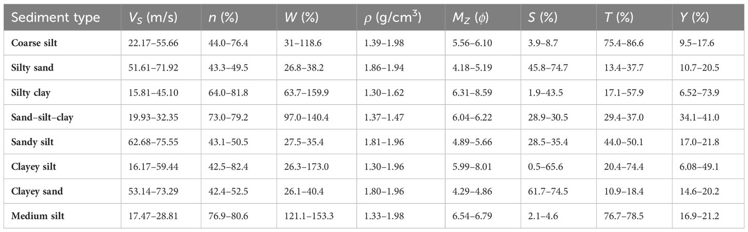
Table 1 Measurement results of shear wave speed and physical parameters of sediment samples in the study area.

Shear wave speed prediction based on the XGBoost algorithm

XGBoost algorithm

eXtreme Gradient Boosting (XGBoost) is an integrated learning algorithm based on the Gradient Boosting Decision Tree (GBDT) algorithm. The basic idea of the XGBoost is to train a new model based on the errors in the old model, which is a weak classifier, generate a series of models in an iterative serial fashion, and sum these models in a linearly weighted fashion to form a powerful integrated model which is a strong classifier (Qian et al., 2020). The XGBoost algorithm introduces a regularization term, which controls the complexity of the model and prevents overfitting (Chen and Guestrin, 2016). In addition, the XGBoost algorithm has higher efficiency for optimal solutions because it performs second-order Taylor expansions on the loss function, while traditional GBDT only utilizes first-order derivative information (Li et al., 2018). So, the XGBoost algorithm was chosen to build the prediction model of the shear wave speed. For the XGBoost algorithm, the dataset for training to build the integrated model is assumed to have n samples and m features, and the ith sample of the training dataset can be represented as (x_i,y_i). Here, x_i denotes the feature vector of the ith sample, representing the physical parameters of sediments, and y_i denotes the label of the ith sample, representing the shear wave speed of sediments. After K iterations, the predicted value ($Y_i^K$) of the integrated model for the ith sample can be expressed as:

$\begin{array}{ll}{Y}_i^K=\sum _{k=1}^K{T}_k(x_i)& (1)\end{array}$

In Equation 1, T_k(x_i) denotes the function that maps the features to the weights of the leaf nodes of the tree structure, which can be expressed as T_k(x_i) = w_q(xi). $w$ is the weight of the leaf nodes. q(x_i) denotes the position of the ith sample in the K decision trees. The objective function of the XGBoost algorithm is:

$\begin{array}{ll}Ob{j}^K=\sum _{i=1}^{n}l(y_i,Y_i^K)+\sum _{k=1}^K\mathit{\Omega }(T_k)& (2)\end{array}$

In Equation 2, $l(y_i,Y_i^k)$ is the loss function representing the error between the predicted values from the model and the real values for the ith sample. ${\sum }_{k=1}^k\mathit{\Omega }(T_k)$ is the regularization item, which is used to limit the number of leaf nodes to prevent the fitting phenomenon in the training process. It can be expressed as:

$\begin{array}{ll}\mathit{\Omega }(T_k)=\mathit{\gamma }T+\frac{1}{2}\mathit{\lambda }\sum _{j=1}^T{w}_j^2& (3)\end{array}$

In Equation 3, γ is the learning rate used to control the number of leaf nodes. T is the number of young leaf nodes. λ is a regular parameter used to control the score of the leaf node.

The XGBoost model is a front-oriented distribution algorithm, and the iterative form of the target function can be expressed as:

$\begin{array}{ll}Ob{j}^K=\sum _{i=1}^{n}l\left(y_i,Y_i^{K-1}+T_K(x_i)\right)+\mathit{\Omega }(T_K)& (4)\end{array}$

In order to find the minimum value of the target function, the second order of (Equation 4) Taylor at T_k = 0 is:

$\begin{array}{ll}Ob{j}^K=\sum _{i=1}^n\left[l(y_i,Y_i^{K-1})+g_i{T}_K(x_i)+\frac{1}{2}{h}_i{(T_K(x_i))}^2\right]+\mathit{\Omega }(T_K)& (5)\end{array}$

$\begin{array}{ll}{g}_i=\frac{\mathit{\partial }l(y_i,Y_i^{K-1})}{\mathit{\partial }{Y}_i^{K-1}}& (6)\end{array}$

$\begin{array}{ll}{h}_i=\frac{{\mathit{\partial }}^{2}l(y_i,Y_i^{K-1})}{{\mathit{\partial }}^2{Y}_i^{K-1}}& (7)\end{array}$

In Equation 5, g_i is the first-order guide, calculated by Equation 6; h_i is the second order guide, calculated by Equation 7.

XGBoost achieves the generation of the learning device by optimizing the structured losses and improves the performance of the algorithm by utilizing the first-order and second-order derivative values of the loss function and through preorder and weighted seminars. Substituting the regularization term expression into Equation 5, the final minimum value of the objective function is obtained, as in Equation 8.

$\begin{array}{ll}Ob{j}^{*}=-\frac{1}{2}\sum _{m=1}^k\left(\frac{G_m^2}{H_m+\lambda }\right)+\mathit{\gamma }T& (8)\end{array}$

The smaller the target function, the smaller the gap between the real values and the model-predicted values, and the better the model fit.

Characteristic parameter selection

After removing outliers and missing values, a total of 226 datasets were obtained, and eight parameters were included in each set: shear wave speed at 2 kHz, sediment n, w, ρ, M_Z, S, T, and Y. Thus, the dimension of the sample data is (226, 8). The number of data samples is similar to that used to predict sediment sound speed based on the machine learning algorithm in the following literature (Hou et al., 2019; Hou et al., 2023; Chen et al., 2022, 2023) and can be used to train the machine learning prediction model for predicting shear wave speed of seafloor sediments.

In machine learning, the Pearson correlation coefficient is commonly used for feature selection, which helps us find the features with high correlation in the dataset, reducing the number of features, improving the generalization ability of the model, and reducing the computation time (Qi et al., 2023). The Pearson correlation coefficient was used to determine the correlation between the sediment shear wave speed and physical parameters. If the coefficient is negative, it means that the two features are negatively correlated, and if the coefficient is positive, the two features are positively correlated. The closer the absolute value of the coefficient is to 1, the greater the degree of correlation. The Pearson correlation coefficient between X and Y variables can be expressed by Equation 9.

$\begin{array}{ll}{\mathit{\rho }}_{X,Y}=\frac{E(XY)-E(X)E(Y)}{\sqrt{E(X^2)-E^2(X)}\sqrt{E(Y^2)-E^2(Y)}}& (9)\end{array}$

The Pearson correlation coefficient of the physical parameters and shear wave speed was calculated for the 226 sets of data, and the correlation coefficients of seafloor sediment shear wave speed with n, w, ρ, M_Z, S, T, and Y are −0.88, −0.81, 0.86, −0.76, −0.55, 0.15, and 0.48, respectively, as shown in Figure 1. According to Figure 1, the n, w, ρ, and M_Z have high correlation coefficients with the shear wave speed and are selected as the input parameters for the model.

Figure 1

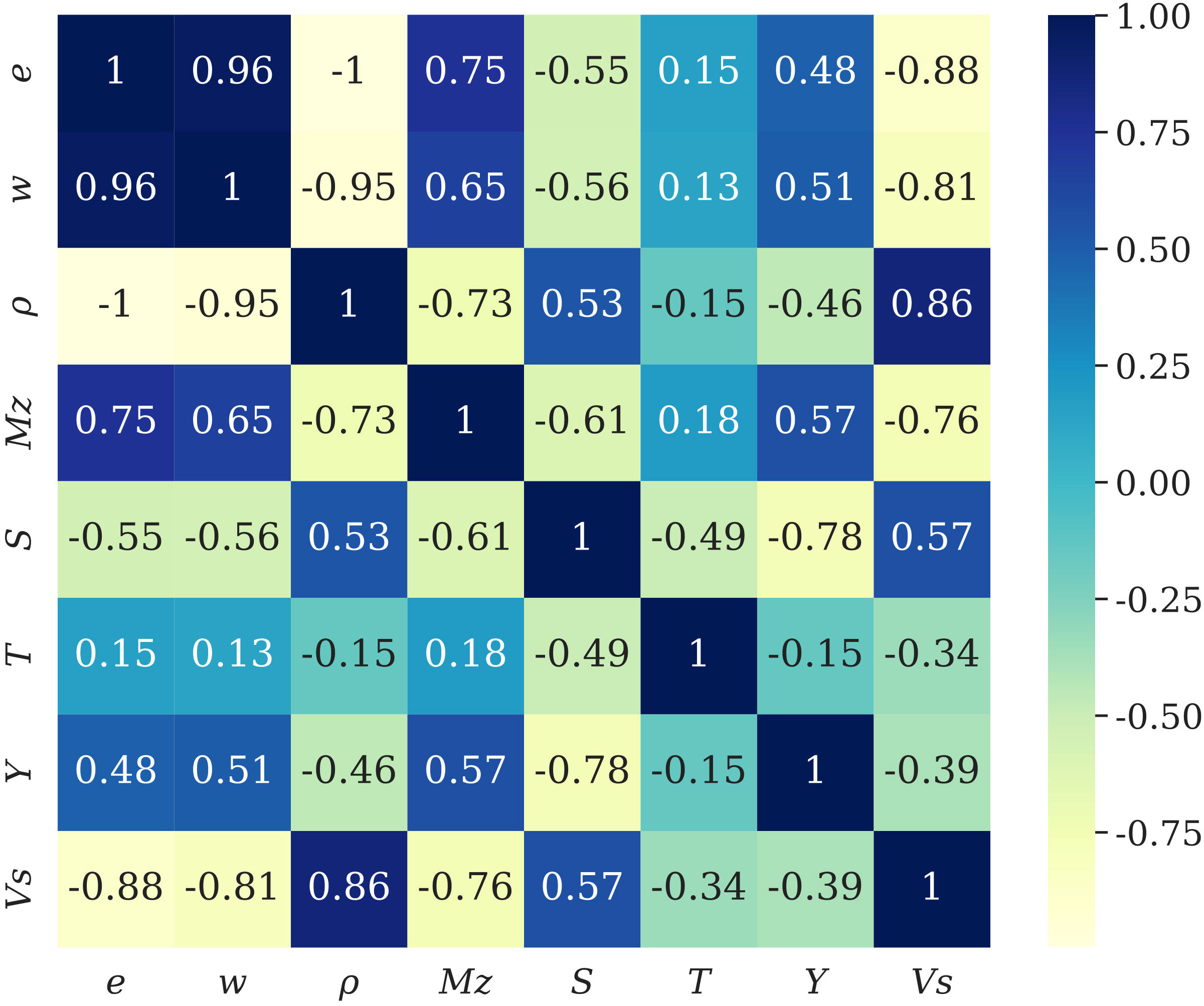
Figure 1 Pearson correlation coefficient matrix for each factor. The last column shows the Pearson correlation coefficient between the shear wave speed of the sediments and physical parameters.

Dataset segmentation

Four physical parameters and the shear wave speed are selected to participate in the subsequent model establishment, and the dimension of the sample data is (226, 5). Firstly, the sample is divided into two parts: one part is used for model building, and the other part is not involved in model building and is used for testing after model building. Subsequently, the dataset used for model building is divided into a training dataset and a validation dataset. The training dataset is used to establish the initial hyperparameters of the model. The validation dataset is used to adjust the hyperparameters in XGBoost in the model to prevent overfitting and select the optimal model. The test dataset is used to evaluate the performance of the model through a comparison between the measured shear wave speed and the prediction of the model. Using random numbers, 166 datasets are randomly selected for model training with a data dimension of (166, 5), 30 datasets are randomly selected for model validation with a data dimension of (30, 5), and the remaining 30 datasets are randomly selected for model testing with a data dimension of (30, 5). As shown in Figure 2, the sediment types in the study area are diverse, and the physical properties and shear wave speeds of different sediment types are different. The datasets of training data, validation data, and test data all contain multiple sediment types, which can ensure the applicability of the model to different types of sediments.

Figure 2

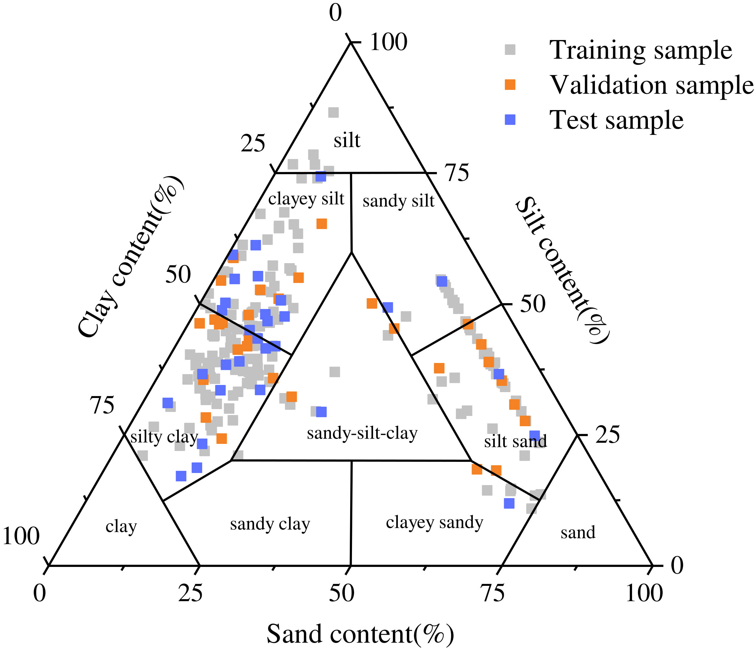
Figure 2 Sediment triangulation map of dataset delineation results in this paper. The gray data points in the figure represent the training data, the orange data points represent the validation data, and the blue data points represent the test data.

Results

Indicators for assessing the results of model predictions

The mean absolute error (MAE), mean absolute percentage error (MAPE), and goodness of fit (R²) are selected as indicators to evaluate the predictive ability. The MAE and MAPE reflect the mean absolute error and mean absolute percentage error between the predicted values and the real values, respectively. R² reflects the degree of goodness of fit of the model. They are expressed as:

$\begin{array}{ll}MAE=\frac{1}{n}\sum _{i=1}^n\left|y_i-Y_i\right|& (10)\end{array}$

$\begin{array}{ll}MAPE=\frac{100\%}{n}\sum _{i=1}^n\left|\frac{y_i-Y_i}{y_i}\right|& (11)\end{array}$

$\begin{array}{ll}{R}^2=1-\frac{{\sum }_{i=1}^n{(Y_i-y_i)}^2}{{\sum }_{\text{i}=1}^{\text{n}}{(\overline{y_i}-y_i)}^2}& (12)\end{array}$

In Equations 10–12, n is the number of the sample, Y_i is the predicted value, y_i is the real value, and $\overline{y_i}$ is the mean of the real values.

Model building and optimization

At first, the 166 sets of training data were substituted into the model for training by using the default hyperparameters in XGBoost to train the data, which was called Model0. Substituting the validation data into Model0, the validation goodness of fit of Model0 was 0.902, and the MAE and MAPE between the validation data and the real values were 3.926 m/s and 12.2%, respectively. In order to obtain a better fitting effect, some hyperparameters were adjusted using a random search method and crossvalidation function. The results are shown in Table 2. The adjusted parameters were entered into the model, and the model was retrained, which was called Model1. Now, the MAE, MAPE, and R² for the validation data were 3.41 m/s, 10.1%, and 0.913, respectively. Compared with the results of Model0, the prediction performance of Model1 was improved with a smaller MAE and higher R².

Table 2

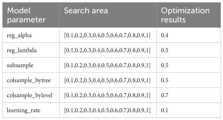
Table 2 Optimization results for the hyperparameters of the random search section.

In addition to the hyperparameters mentioned above, two other hyperparameters, n_estimators and max_depth, are very important for the accuracy of the model training. The n_estimators indicates the number of weak learners (regression trees) in the model; a smaller number of learners will lead to insufficient model performance, and a larger number may improve model performance but will increase training time and memory consumption. The max_depth parameter indicates the maximum depth of the tree, specifying the weak learners. A deeper tree can capture more complex interactions between the features, but the deeper the tree, there greater the risk of overfitting. The n_estimators and max_depth were manually adjusted and optimized according to the curves of MAE changing with the n_estimators and max_depth for the training and validation sets, shown in Figures 3, 4, respectively. As shown in Figure 3, when the value of n_estimators is 115, the MAE of the validation data and the real values are the smallest. As shown in Figure 4, when the value of max_depth is 6, the MAE is the smallest.

Figure 3

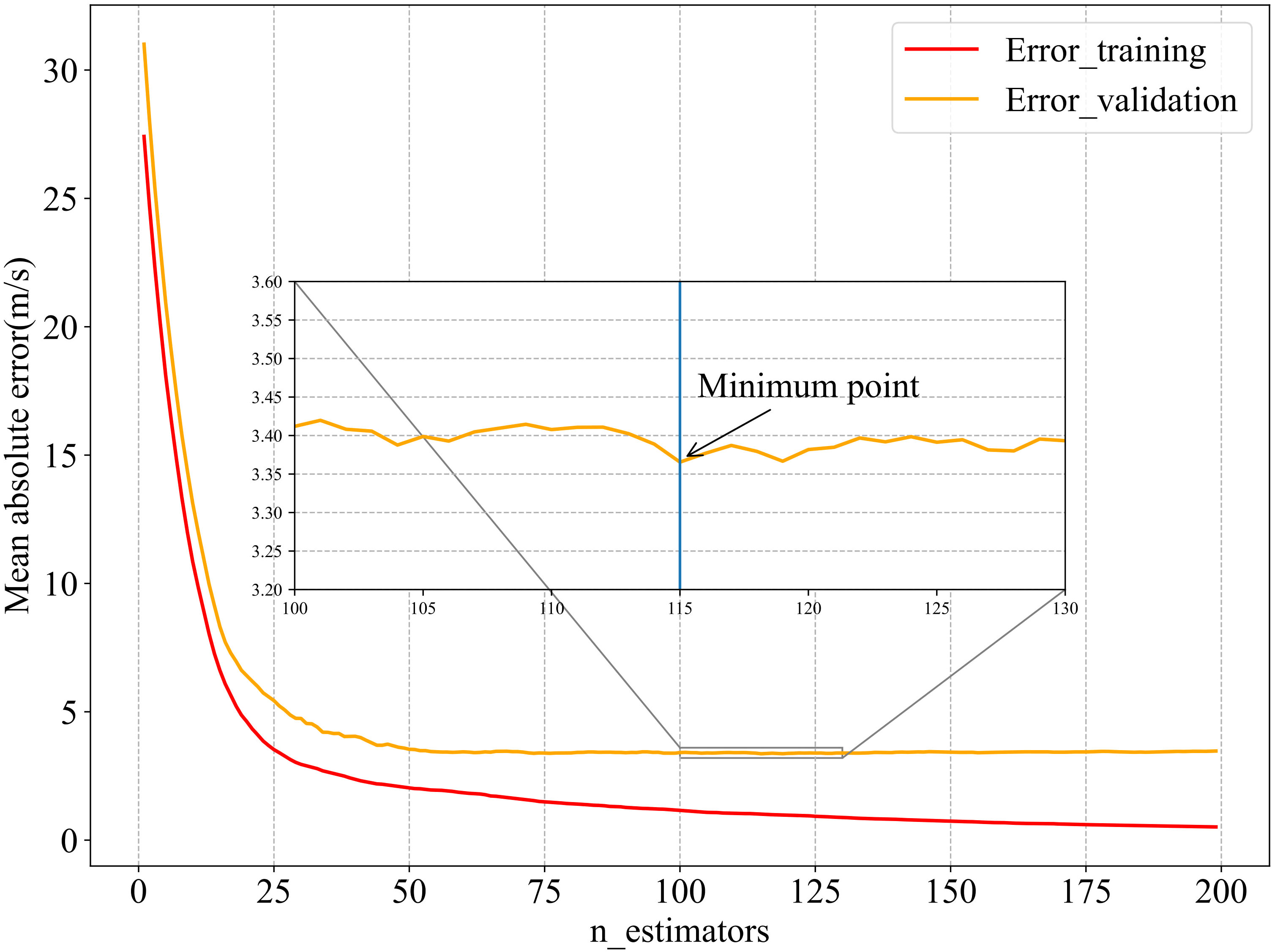
Figure 3 Trend of MAE with n_estimators hyperparameter in model training and validation. The red solid line is the iteration change of the model training error, and the orange solid line is the iteration change of the validation result error.

Figure 4

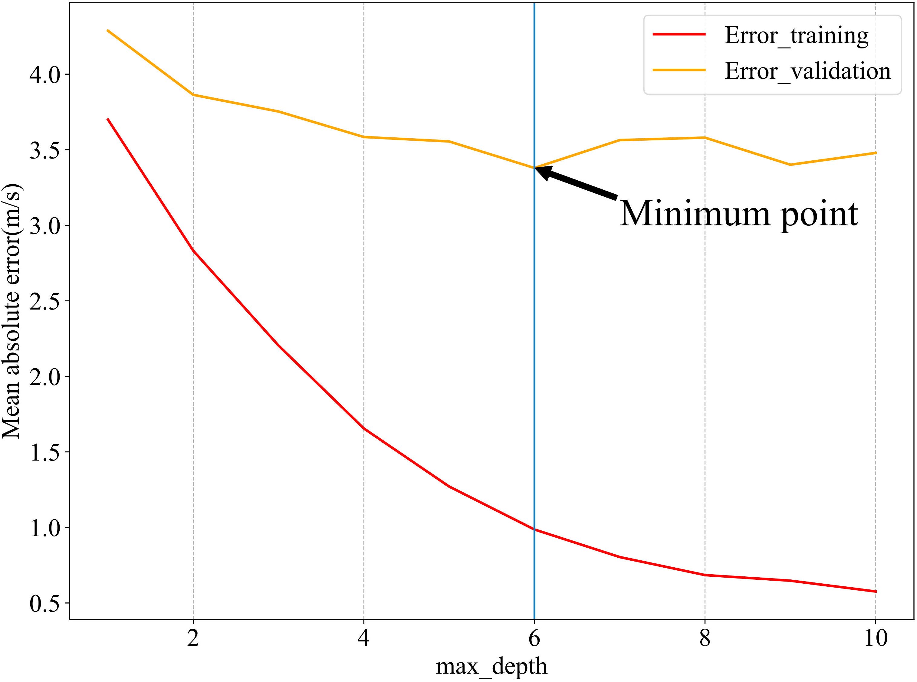
Figure 4 Trend of MAE with max_depth hyperparameter in model training and validation. The red solid line is the iteration change of the model training error, and the orange solid line is the iteration change of the validation result error.

The value of the hyperparameters of the XGBoost model was finally obtained through the adjustment and optimization using the random search, crossvalidation function, and manual optimization. When the adjusted parameters were substituted into the model, it was the best-fitted model for the prediction of the shear wave speed in the study area and can be called Model2. The coefficient of determination of the validation data was 0.914, and the MAE and MAPE of the predicted values of the training data and the measured data were 3.366 m/s and 9.90%, respectively. Figure 5 shows the comparison between the model’s predicted values and the real values. The predicted data are closely matched with the real data, and the multiparameter shear wave speed prediction model constructed based on the XGBoost algorithm has a small difference between the predicted values and the real values, and the model prediction accuracy is high.

Figure 5

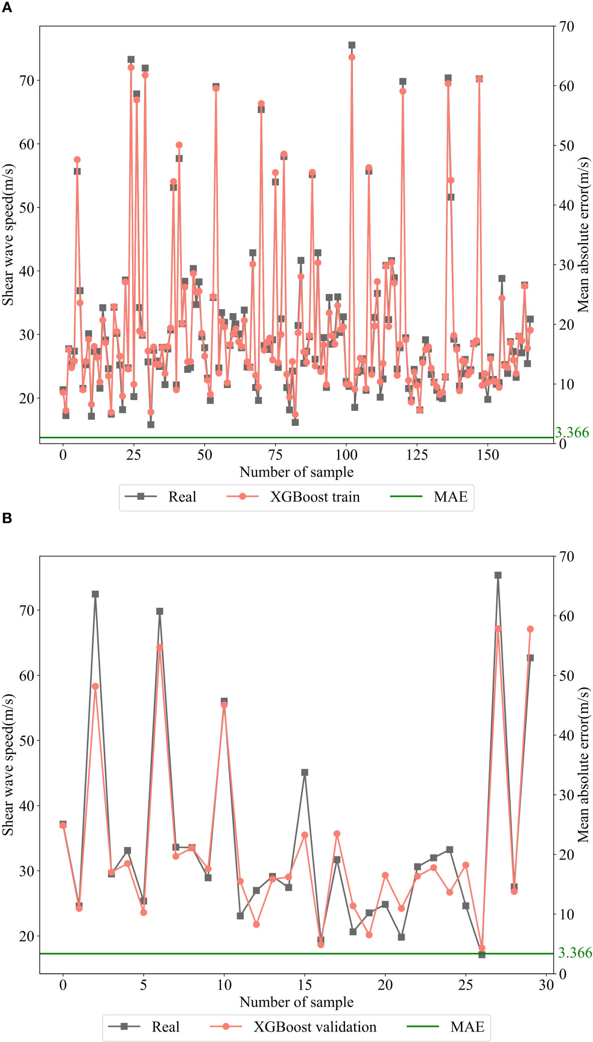
Figure 5 Comparison of predicted and real values: (A) 166 sets of training sample; (B) 30 sets of validation sample. The solid green line represents the MAE between each prediction value and the real values.

Analysis of the contribution of characteristic parameters

Lundberg and Lee (2017) proposed the SHapley Additive exPlanations (SHAP) method to explain the machine learning model and evaluated the importance of features by calculating the average value of the absolute value of each feature in the sample data. Figure 6 shows the average value of the absolute SHAP value of each feature variable as the importance of this feature. It can be seen that the main influencing factors on shear wave speed in the XGBoost model are porosity and water content, followed by density and average grain size.

Figure 6

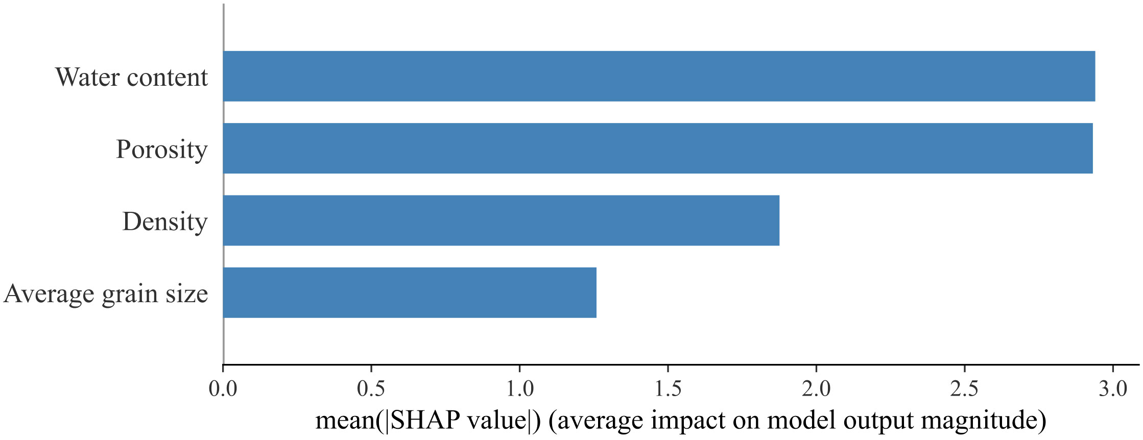
Figure 6 Ranking the average influence values of the model output.

Discussion

In order to analyze the predictive performance of the multiparameter shear wave speed prediction model based on the XGBoost algorithm, the following section will use the same 166 sets of training data to build the single- and dual-parameter prediction models and the GS prediction model and compare the prediction errors and the magnitude of the coefficients of determination of the models.

Single-parameter prediction model

The 166 sets of training data were used to establish four single-parameter prediction models. The mathematical relationship between the physical parameters of the sediment and the shear wave speed was fitted using the least squares method to establish the corresponding single-parameter empirical equations listed in Table 3. As shown in Table 3, the shear wave speed has high correlations with the porosity, water content, density, and average grain size, whose goodness of fit is all greater than 0.66. The predicted shear wave speed using the single-parameter prediction equations in Table 3 and the real values are compared and shown in Figure 7. According to Figure 7 and Table 3, the MAEs of the single-parameter prediction equations are all higher than 5 m/s, and the prediction equation based on porosity is the lowest with an MAE of 5.014, while that of the prediction equation based on average grain size is the highest with an MAE of 5.427.

Table 3

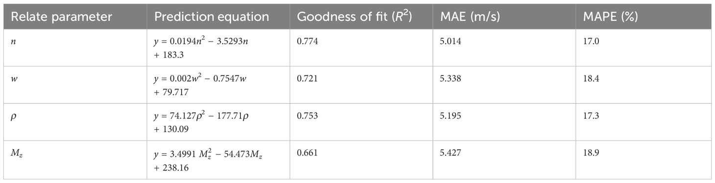
Table 3 Single-parameter prediction models.

Figure 7

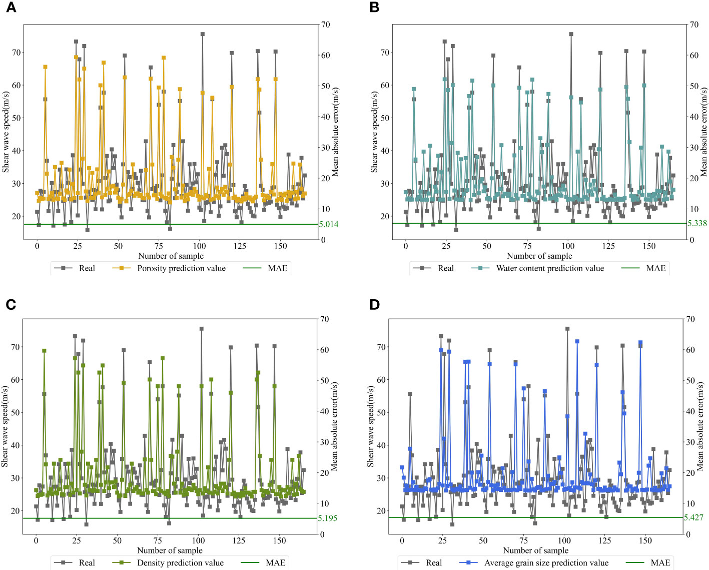
Figure 7 Comparison of predicted shear wave speed from the single-parameter prediction models with real values: (A) porosity, (B) water content, (C) density, and (D) average grain size. The gray curve in the figures represents the real values. The solid green lines show the MAE between the predicted and real values of the 166 training samples.

Dual-parameter prediction model

The same 166 sets of training data were used to establish six dual-parameter prediction models. The mathematical relationship between the physical parameters of the sediment and the shear wave speed was fitted using the least squares method, and the corresponding dual-parameter empirical equations were established and listed in Table 4. Similarly, the predicted shear wave speed using the dual-parameter prediction equations in Table 4 and the real values are compared and shown in Figure 8. The results show that the goodness of fit of the dual-parameter prediction equations is all greater than 0.78, which is higher than that of the single-parameter prediction equations established in this paper. The MAEs of the dual-parameter prediction equations are all less than 4.8 m/s, which is lower than that of the single-parameter equations. This indicates that the dual-parameter equations have a higher prediction accuracy than the single-parameter equations.

Table 4

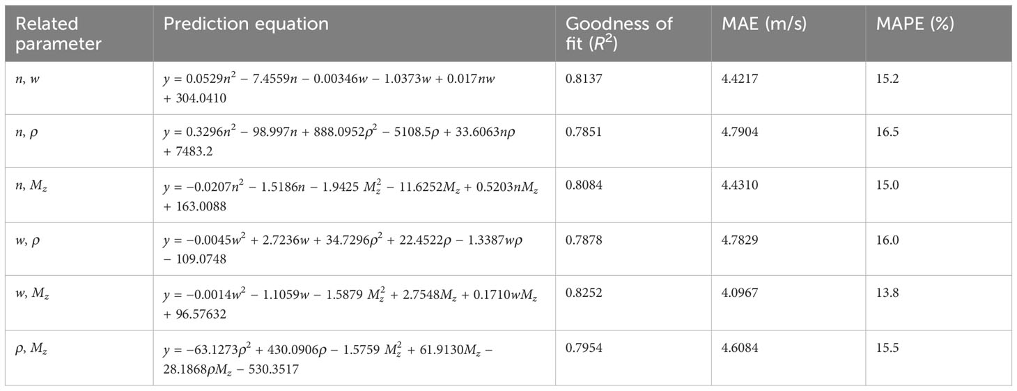
Table 4 Dual-parameter prediction models.

Figure 8

Figure 8 Comparison of predicted shear wave speed from the dual-parameter prediction models with real values: (A) porosity—water content, (B) porosity—density, (C) porosity—average grain size, (D) water content—density, (E) water content—average grain size, and (F) density—average grain size. The gray curve in the figures represents the real values, and the solid green lines show the mean absolute error between the predicted and real values of the 166 training samples.

GS model

In recent years, researchers have studied the propagation mode of sound waves in sediments and summarized models for predicting sound speed in different theoretical media. Buckingham (1997) proposed the grain-shearing (GS) model, which introduced the sticky-slip mechanism between sediment grains, and believed that saturated, unconsolidated particle media have dual properties of fluid and elastic solid, and grains do not cement each other although they contact each other. Furthermore, it is believed that the stiffness of the sediment is generated by the mutual sliding of the grains, and the stiffness supports the existence of shear waves in the sediment. The equation for calculating the shear wave speed is as follows:

$\begin{array}{ll}{V}_s=\sqrt{\frac{{\gamma }_s}{\rho }}\frac{{(\omega T)}^{\frac{n}{2}}}{cos(\frac{n\pi }{4})}& (13)\end{array}$

Where, γ_s is the shear stiffness coefficient, which is used to describe the viscous sliding mechanism and characterize the shear action between grains, calculated by Equation 14. ρ is the density of deposited objects, calculated by Equation 15. ω is the angular frequency. T is any time variable, which can be set to 1 s. n is the strain hardening index, which represents the strain hardening degree of intergranular contact when sediment grains slip.

$\begin{array}{ll}{\mathit{\gamma }}_s={\mathit{\gamma }}_{s0}{\left(\frac{(1-\mathit{\beta })u_{g}d}{(1-{\mathit{\beta }}_0)u_{g0}{d}_0}\right)}^{\frac{2}{3}}& (14)\end{array}$

Where, γ_s0 is the initial value of γ_s. β, u_g, and d represent measured sediment fraction porosity, grain size, and buried depth, respectively. β₀, u_g0, and d₀ are the reference values of fractional porosity, grain size, and buried depth of sediments, and the specific values are shown in Table 5.

Table 5

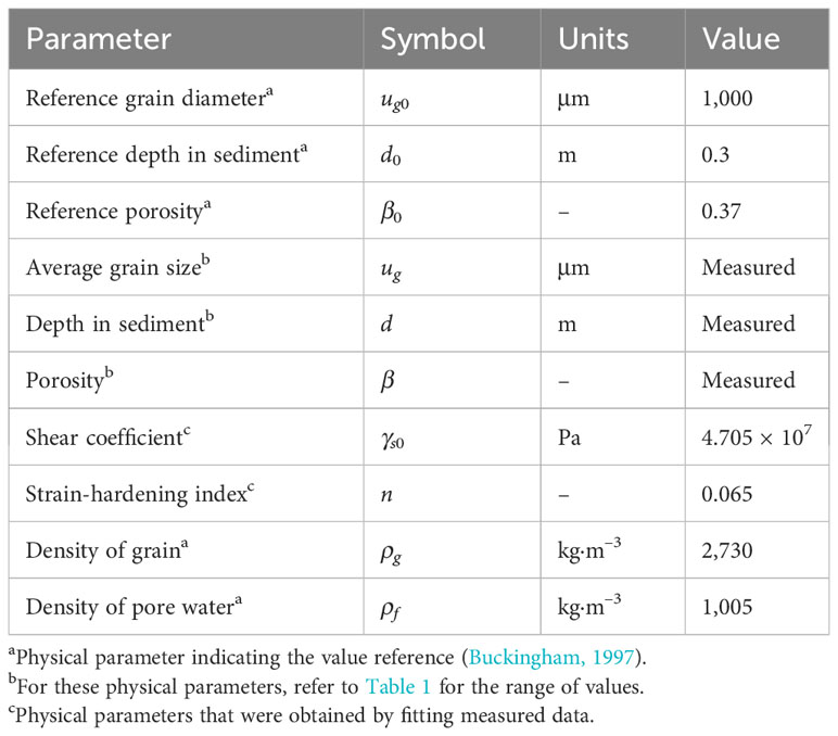
Table 5 Input parameters of GS model.

$\begin{array}{ll}\mathit{\rho }=(1-\mathit{\beta })*{\mathit{\rho }}_g+\mathit{\beta }*{\mathit{\rho }}_f& (15)\end{array}$

$\begin{array}{ll}{u}_g=2^{-\mathit{\varphi }}& (16)\end{array}$

Where, ρ_g is the particle density, ρ_f is the pore fluid density, and ϕ represents the grain size in Equation 16; here, the average grain size of the sediment is selected.

The 166 sets of training data are substituted into Equation 13 to obtain the minimum value of the mean absolute error between the predicted and real values of the shear wave speed, which leads to the optimal values of the shear coefficient and strain hardening index. The values of the input parameters of GS for best fitting are shown in Table 5. Substituting the parameter values into the model, the results of the predicted and real values are shown in Figure 9. The goodness of fit of the model was 0.678; the MAE and MAPE between the real values and the predicted values were 5.253 m/s and 18.09%, respectively.

Figure 9

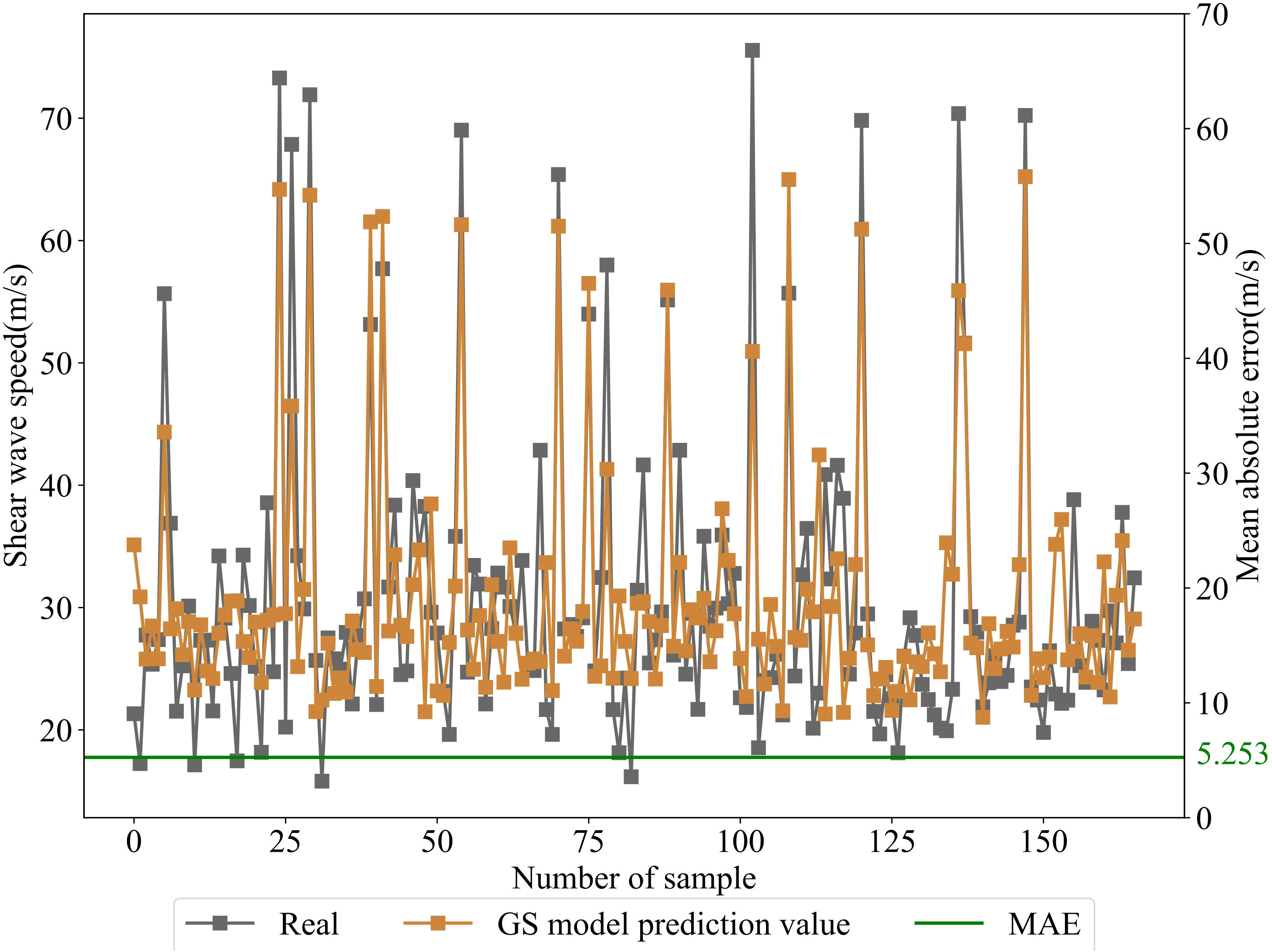
Figure 9 Comparison of predicted shear wave speed from the GS model with real values. The gray curve in the figure represents the real values, the brown curve represents the adjusted GS model predicted values, and the solid green lines show the mean absolute error between the predicted and real values of the 166 training samples.

Comparison of predicted results of each model

To check the accuracy of model fitting, 30 groups of test data that were not involved in model building were substituted into each prediction model, and the difference between the predicted values and the real values of different models was analyzed. The MAEs and the MAPEs between the predicted values and the real values of each model were calculated, and the results are shown in Figure 10. It can be seen that the XGBoost model has the smallest MAE and MAPE and the highest goodness of fit compared to the single-parameter prediction models, dual-parameter prediction models, and GS prediction model.

Figure 10

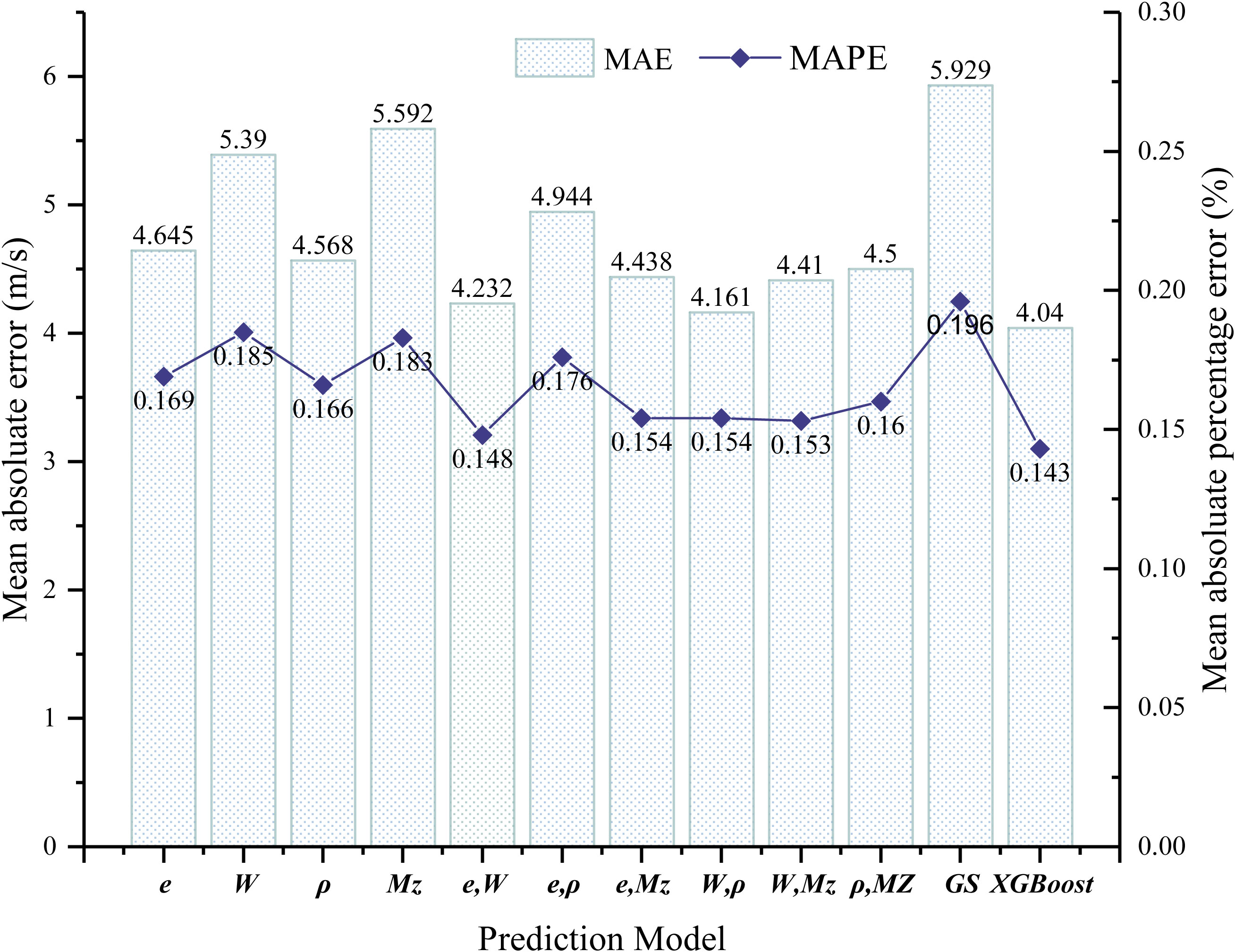
Figure 10 Comparison of the error of predicted results of 30 groups of test data substituted into each model.

Conclusions

In this paper, using the seafloor sediments obtained in the northern part of the South China Sea, the correlation between the sediment shear wave speed and the physical properties was investigated, the multi-parameter shear wave speed prediction model based on the XGBoost algorithm was established, and the predicted results of the XGBoost model were compared with the single- and dual-parameter models and the GS model. The conclusions are summarized as follows:

(1) The shear wave speed of shallow sediments in the study area has a good correlation with porosity, water content, density, and average grain size. By optimizing the hyperparameters of the model, the best fit of the XGBoost algorithm is obtained when the n_estimator and max_depth are 115 and 6, respectively. The mean absolute error and the goodness of fit between the predicted values and validation data are 3.366 m/s and 9.90%, respectively.

Compared with the single-parameter prediction models, the dual-parameter prediction models, and the GS prediction model, the multiparameter shear wave speed prediction model based on the XGBoost algorithm has the lowest MAE and MAPE between the test data and the predicted values, which are 4.04 m/s and 14.3%, respectively. It indicates that the multiparameter shear wave speed prediction model based on the XGBoost algorithm has a higher accuracy for predicting the shear wave speed in this area (2).

Data availability statement

The raw data supporting the conclusions of this article will be made available by the authors, without undue reservation.

Author contributions

WM: Writing – original draft, Writing – review & editing. XM: Writing – review & editing. JW: Writing – review & editing. GL: Writing – review & editing. BL: Writing – review & editing. GK: Writing – original draft, Writing – review & editing. JL: Writing – review & editing. LZ: Writing – review & editing. PZ: Writing – review & editing.

Funding

The author(s) declare financial support was received for the research, authorship, and/or publication of this article. This study was supported by the National Key R&D Program of China under Grant No. 2021YFF0501200, in part by the Central Public-Interest Scientific Institution Basal Research Fund under Grant No. GY0220Q09, and in part by the National Natural Science Foundation of China under Grant No. U2006202, No. 42376076, and No. 41706062.

Acknowledgments

We thank all those involved in the marine surveys that collected the data used in this study. Thanks to Mujun Chen from Ocean University of China for helpful discussions on machine learning methods.

Conflict of interest

The authors declare that the research was conducted in the absence of any commercial or financial relationships that could be construed as a potential conflict of interest.

Publisher’s note

All claims expressed in this article are solely those of the authors and do not necessarily represent those of their affiliated organizations, or those of the publisher, the editors and the reviewers. Any product that may be evaluated in this article, or claim that may be made by its manufacturer, is not guaranteed or endorsed by the publisher.

References

Buckingham M. J. (1997). Theory of acoustic attenuation, dispersion, and pulse propagation in unconsolidated granular materials including marine sediments. J. Acoustical Soc America 102 (5), 2579–2596. doi: 10.1121/1.420313

CrossRef Full Text | Google Scholar

Buckingham M. J. (2005). Compressional and shear wave properties of marine sediments: comparisons between theory and data. J. J. Acoustical Soc. America 1171, 137–152. doi: 10.1121/1.1810231

CrossRef Full Text | Google Scholar

Chen T., Guestrin C. (2016). XGBoost: A scalable tree boosting system. [C]// Proceedings of the 22nd ACM SIGKDD International Conference on Knowledge Discovery and Data Mining, August 13 -17, 2016, San Francisco, California. New York: ACM, 2016:785–794. doi: 10.1145/2939672.2939785

CrossRef Full Text | Google Scholar

Chen M. J., Meng X. M., Kan G. M., Wang J. Q., Li G. B., Liu B. H., et al. (2022). Predicting the sound speed of seafloor sediments in the east China sea based on an XGBoost algorithm. J. J. Mar. Sci. Eng. 10 (10), 1366. doi: 10.3390/jmse10101366

CrossRef Full Text | Google Scholar

Chen M. J., Meng X. M., Kan G. M., Wang J. Q., Li G. B., Liu B. H., et al. (2023). Predicting the sound speed of seafloor sediments in the middle area of the Southern Yellow Sea based on a BP neural network model. J. Mar. Georesour. Geotechnol. 41 (6), 662–670. doi: 10.1080/1064119X.2022.2085216

CrossRef Full Text | Google Scholar

Guo X. S., Liu X. L., Li M. Q., Lu Y. (2023). Lateral force on buried pipelines caused by seabed slides using a CFD method with a shear interface weakening model. J. Ocean Eng. 280, 114663. doi: 10.1016/j.oceaneng.2023.114663

CrossRef Full Text | Google Scholar

Hou Z. Y. (2016). The Correlation of Seafloor Sediment Acoustic Properties and Physical Parameters in the Southern South China Sea (Chinese Academy of Sciences: Institute of Oceanology).

Google Scholar

Hou Z. Y., Wang J. Q., Chen Z., Yan W., Tian Y. H. (2019). Sound velocity predictive model based on physical properties. Earth and Space Science 6, 1561–1568. doi: 10.1029/2018EA000545

CrossRef Full Text | Google Scholar

Hou Z. Y., Wang J. Q., Li G. B. (2023). A sound velocity prediction model for seafloor sediments based on deep neural networks. J. Remote Sens. 15, 4483. doi: 10.3390/rs15184483

CrossRef Full Text | Google Scholar

Jackson D. R., Richardson M. D. (2007). High-frequency seafloor acoustics (New York: Springer).

Google Scholar

Kan G. M., Cao G. L., Wang J. Q., Li G. B., Liu B. H., Meng X. M., et al. (2020). Shear wave speed of shallow seafloor sediments in the northern South China Sea and their correlations with physical parameters. J. Earth Space Sci. 7 (3). doi: 10.1029/2019ea000950

CrossRef Full Text | Google Scholar

Kan G. M., Zhang Y. F., Su Y. F., Li G. B., Meng X. M. (2014). Shear wave speeds measured for sediments from the middle of the southern Yellow Sea and their correlation with physical-mechanical parameter. J. Adv. Mar. Sci. (in Chinese) 32 (03), 335–342. doi: 10.3969/j.issn.1671-6647.2014.03.005

CrossRef Full Text | Google Scholar

Li Y. Z., Wang Z. Y., Zhou Y. L., Han X. Z. (2018). Improvement and application of xgboost algorithm based on Bayesian optimization. J. J. Guangdong Univ. Technol. 35 (01), 23–28. doi: 10.12052/gdutxb.170124

CrossRef Full Text | Google Scholar

Lu B., Li G. X., Huang S. J. (2004). A preliminary study of shear wave in seafloor surface sediments. J. J. Trop. Oceanogr. (in Chinese) 23 (4), 11–18. doi: 10.1080/1064119x.2022.2085216

CrossRef Full Text | Google Scholar

Lu B., Liang Y. B. (1991). Correlation between sound velocity and physical-mechanical parameters of marine sediments. J. Trop. Ocean 10 (3), 96–100.

Google Scholar

Lundberg S., Lee S. I. (2017). A unified approach to interpreting model predictions. 31st Annual Conference on Neural Information Processing Systems Vol. 30 (Long Beach: NIPS), 4768–4777.

Google Scholar

Pan G. F., Ye Y. C., Lai X. H. (2006). Shear wave speed of seabed sediment from laboratory measurements and its relationship with physical properties of sediment. J. Acta Oceanol. Sin. (in Chinese) 28 (5), 64–68. doi: 10.3321/j.issn:0253-4193.2006.05.008

CrossRef Full Text | Google Scholar

Qi W., Sun R., Zheng T., Qi J. (2023). Prediction and analysis model of ground peak acceleration based on XGBoost and SHAP. J. Chin. J. Geotech. Eng. 45 (09), 1934–1943. doi: 10.11779/CJGE20220417

CrossRef Full Text | Google Scholar

Qian N., Wang X. S., Fu Y. C., Zhao Z. C., Xu J. H., Chen J. J. (2020). Predicting heat transfer of oscillating heat pipes for machining processes based on extreme gradient boosting algorithm. J. Appl. Thermal Eng. 164, 114521. doi: 10.1016/j.applthermaleng.2019.114521

CrossRef Full Text | Google Scholar

Richardson M. D., Briggs K. B. (1996). In situ and laboratory geoacoustic measurements in soft mud and hard-packed sand sediments: Implications for high-frequency acoustic propagation and scattering. J. Geo Marine Lett. 16 (3), 196–203. doi: 10.1007/BF01204509

CrossRef Full Text | Google Scholar