Geospatial analysis of shoreline changes in the Oman coastal region (2000-2022) using GIS and remote sensing techniques

This research introduces an innovative method employing the Canny edge detector for automatic and precise coastline extraction, aiming to analyze spatial and temporal variations in the Oman coastline from 2000 to 2022 using GIS and remote sensing (RS) techniques. Focusing on both multi-decadal and short-term periods, the study aims to detect accretion and erosion rates through the observation and interpretation of coastal changes. Utilizing the Digital Shoreline Analysis System and LANDSAT imageries, Shoreline changes have been quantitatively evaluated using three distinct approaches: Linear Regression Rate (LRR), End Point Rate (EPR), and Net Shoreline Movement (NSM). The dynamic nature of the Oman coastal region necessitates a comprehensive understanding of its evolving coastline. Our investigation applies digital shoreline analysis to discern shifts in the coastline’s position, employing a multiple regression approach for quantifying the rate of coastal change. To facilitate automatic shoreline extraction, various methods were experimented with, ultimately determining the Canny Edge algorithm’s superiority in yielding precise results. The paper outlines the monitoring procedures for the coastal area and analyzes coastline changes using geospatial techniques. This analysis provides valuable insights for the planning and management of the Oman shore. Furthermore, the proposed model’s applicability is rigorously tested against other generic edge detection algorithms, including Sobel, Prewitt, and Robert’s techniques. The conclusive findings demonstrate that our model outperforms these alternatives, particularly excelling in the accurate detection of the coastline. This research contributes to a deeper understanding of coastal dynamics and offers a robust methodology for coastal monitoring, with implications for effective planning and management strategies in the Oman shore region.

1 Introduction

Over time, coastal usage areas are continually changing. It is imperative to constantly redefine and monitor coastal areas in light of this change. The coastal usage area changes as a result of events such as drifting coastal soil into the sea, waves that carry soil to the shore, deltas that form along the river directly affecting the shore, natural changes resulting from the region’s geographical location, and sea level changes (Parthasarathy and Deka, 2019; Apostolopoulos and Nikolakopoulos, 2021; Rahman et al., 2022; Nidhinarangkoon et al., 2023). A premier factor in coastal change is the effects of natural events. When coastal cities are examined, it is the changes caused by natural events that are the most significant. As a result of the settlements on the coasts, natural events are triggered, and erosion is a common consequence of the sea’s progression to land. Thus, the coastal city can transform over time (Gurel, 2018).

In coastal planning, coastal management, and decision-making processes, it is imperative to take into account the physical and socioeconomic impacts of coastal areas (Dasgupta et al., 2009; Gazioğlu et al., 2010; Yasir et al., 2020a; Yasir et al., 2020b; Hossain et al., 2021; Yasir et al., 2021). Coastal management and engineering design rely on essential information to predict the coastline’s past, present, and future locations. Analyzing coastal data is crucial in various aspects, such as coastal protection design (Apostolopoulos and Nikolakopoulos, 2022), the calibration and validation of numerical models (Hanson et al., 1988), assessing sea-level rise (Leatherman, 2001), defining legal property boundaries (Morton and Speed, 1998), and monitoring coastal surveys (Smith and Jackson, 1992). To analyze coastal variability and trends effectively, a clear definition of the “coastline” is indispensable. Given the dynamic nature of this boundary, it is essential to evaluate the selected shoreline definition both in terms of time and space (Boak and Turner, 2005). While a concise and ideal description of the coastline is that it coincides with the physical interface of water and land (Dolan et al., 1980), the application of this definition is challenging. The coastal position continually shifts over time due to sediment movement along the coastline and the dynamic nature of water levels, especially at the coastline, influenced by waves, tides, groundwater, storms, and other factors. Recognizing the significance of defining the “coastline” is crucial for the analysis of coastal variability and trends. Given the dynamic nature of this boundary, a temporal and spatial evaluation of the chosen shoreline definition is imperative (Zheng et al., 2023). The instantaneous shoreline refers to the immediate location of the land-water interface (Mullick et al., 2020; Hui et al., 2022). It is important to acknowledge that the cost is a time-dependent phenomenon with short-term variability. While defining the coastline, it is also necessary to take into account the coastal variations. Most coastal change studies consider discrete transitions or points and monitor how they change over time. Defining the coastline requires consideration of coastal variations as well. In most coastal change studies, discrete transitions or points are considered and their changes are monitored over time. In their study, Eliot and Clarke (1989) demonstrated that a small-scale study of one area of the coastline does not fully reflect the change of the entire coast.

Nowadays, monitoring coastal areas, which are the only areas where the atmosphere, hydrosphere, and earth interact with each other, determining the temporal change, and comparing historical data with current data, coastal area management and monitoring of the change in the coastline are carried out using computer science and remote sensing technologies. RS data has become an indispensable tool in the management and planning of coastal and marine areas (Uçkaç, 1998; Yasir et al., 2024). Knowledge of coastal location is essential for tackling shore issues and measuring and identifying land and water resources such as land area and perimeter of coastlines. Performing this task can be challenging, time-intensive, and at times, unfeasible, especially when employing conventional ground surveying methods over a vast area (Cracknell, 1999; Li and Michiel, 2010; Kuleli et al., 2011). RS data deliver important preliminary estimates of change (Ghaderi and Rahbani, 2020). At the same time, maps obtained from satellite data are a very important resource for reflecting changes in the coastline over the years (Kevin and El Asmar, 1999; Shaghude et al., 2003). Various image processing techniques have been applied to extract water features from satellite images over the past few years. Single-band methods employ a chosen threshold value for watermark removal, but they often encounter errors stemming from the mixing of water pixels with various land cover types (Du et al., 2012).

Classification techniques employed to eliminate surface water typically yield greater accuracy compared to single-band techniques (Du et al., 2012). Multiband approaches amalgamate various reflective bands to enhance the extraction of surface water (Du et al., 2012). For example, the development of the Normalized Difference Water Index (NDWI) aimed to discern water features in Landsat images. However, NDWI often includes false positives arising from built-up terrains. To address this issue, a modified Normalized Difference Water Index (MNDWI) was implemented, substituting the near-infrared (NIR) band for the mid-infrared (MIR) band (Pandey et al., 2023). MNDWI excels in isolating surface water while suppressing inaccuracies stemming from both soil and vegetation, achieved through the removal of surface soil (Pandey et al., 2023). The first article to propose the green and infrared band ratio (NDWI), which reveals the water feature in remote sensing images, belongs to McFeeters (1996).

DSAS is a versatile tool with a wide range of applications, making it valuable for calculating positional changes over time (Baig et al., 2020). It can be used to track alterations in various features, including glacier boundaries in historical aerial photographs, riverbank borders, and shifts in land use/land cover (Saad, 2021). To ensure the consistency and accuracy of computed results, DSAS offers rate-of-change information and mathematical data to assist in shoreline change calculations. The model comprises three primary components. First, it involves defining a baseline. Next, orthogonal transects are generated to indicate spatial separation along the coastline. Finally, rates of change are calculated using diverse approaches or models, such as linear regression rates, endpoint rates, average rates, and more (Adebola et al., 2017). However, it’s worth noting that remote sensing technology plays a pivotal role in cost-effective data acquisition. Optical images are readily interpretable and accessible. Moreover, the unique characteristics of water, vegetation, and soil, including the absorption of infrared waves by water and their strong reflection by vegetation and soil, provide an ideal means of delineating land-water boundaries. These distinctive features have led to the frequent use of images containing infrared bands for shoreline analysis (Alesheikh et al., 2004). The main objective of this paper is as follows;

● To develop an innovative method for automatic and precise coastline extraction, employing the Canny edge detector. Our objective is to analyze the spatial and temporal variations in the Oman coastline from 2000 to 2022 using GIS and RS techniques.

● Our study is centered on the detection of accretion and erosion rates through the observation and interpretation of coastal changes over both multi-decadal and short-term periods.

● The application of digital shoreline analysis allows us to detect shifts in the position of the coastline. A multiple regression approach will be used to quantify the rate of coastal change along the coast of Oman, including EPR, NSM, and LRR.

1.1 Geomorphology and surface processes

Oman’s northeastern Al Batinah coastal plain is surrounded by both the Al Hajar Al Gharbi (Western Hajar) Mountains and the Sea of Oman. Stretching approximately 230 km in an NW-SE direction, from the United Arab Emirates (UAE) border in the northwest to Muscat in the southeast, it forms a crescent shape parallel to the mountains (Figure 1). This shore plain is roughly 50 km wide at its center and tapers at its northwest and southeast ends. Notably, around 90% of its shoreline consists of sandy beaches (Al-Hatrushi et al., 2015). Numerous deltas within the coastal plain drain from the mountains (Lotfy, 2012). The shore plain itself is composed of continuous alluvial fans that have been deposited from the southern highlands. It can be divided into two parts: the alluvial plain and the coastal zone. The gently sloping alluvial plain features surface characteristics dominated by both recent and ancient alluvial fans. The coastal area is situated at an elevation of less than 20 meters above sea level and includes coastal dunes and sabkhas (supratidal mudflats or sandflats) near the shoreline. The coastline is characterized by sandy beaches, numerous tidal inlets, lagoons, and stands of mangroves near the mouths of significant wadis. Sediments along this plain vary from gravel and coarse sands near the mountains to fine sands and silt as one moves closer to the coast (Kwarteng et al., 2016). The Al Batinah watersheds are known for their aridity and susceptibility to rapid wadi flooding, especially during the winter (Abushandi and Abualkishik, 2020). According to Kwarteng et al. (2009), the Al Batinah plain receives an average annual rainfall of 101 millimeters, with air temperatures varying based on elevation. Coastal regions experience higher relative humidity throughout much of the year, particularly in the summer when it can reach up to 99%. The region’s winter weather is influenced by northwesterly and northeasterly winds, while the southwesterly monsoon affects summer conditions. Although there are several groundwater aquifers in the Al Batinah region, they are not extensively utilized due to the risk of saltwater intrusion. The tidal system of Al Batinah’s beaches is primarily influenced by low-wave energy tides and an annual littoral drift of 100,000 m3 (Al-Hatrushi et al., 2015). Furthermore, Al-Hatrushi et al. (2015) express concerns about the vulnerability of the Al Batinah coastline to sea-level rise due to climate change, as well as frequent threats from cyclones and storms like Gonu in 2007 and Kyar in 2019. Air pressure, wind patterns, and precipitation are the key climatic variables strongly correlated with geomorphological processes along the coastline. These mechanisms play a crucial role in sediment deposition, transport, and coastal processes such as erosion. Notably, the main wadis replenish the beach with sediment during periods of precipitation (Kwarteng et al., 2009).

Figure 1

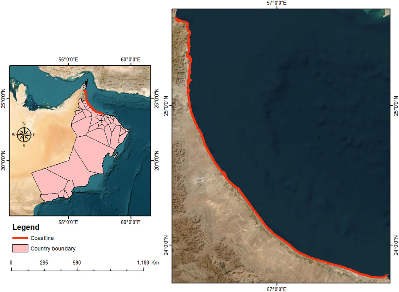
Figure 1 Location map.

2 Materials and methods

2.1 Datasource

In this study, Landsat Multi-temporal satellite data has been utilized, specifically making use of the Operational Land Imager (OLI) and Enhanced Thematic Mapper Plus (ETM+) sensors, to encompass the study period spanning from 2000 to 2022. These satellite images were acquired from the US Geological Survey’s Earth Explorer website (http://earthexplorer.usgs.gov) at no cost. Due to their open accessibility and cost-effectiveness, Landsat images were selected as the most suitable data source for our research. Detailed information about the data used can be found Table 1. The data underwent pre-processing by the USGS before being delivered in the form of level-one terrain-corrected (L1T) Landsat data. These data were provided in the WGS84 geodetic datum and the Universal Transverse Mercator Map projection (UTM, Zone 40N). It is important to note that the L1T nature of the data ensured that radiometric and geometric deformations were rectified before being made available, as discussed by Jensen (1996), Seilheimer et al. (2007), and Nahiduzzaman et al. (2015). Figure 1 shows the location map of the study area.

Table 1

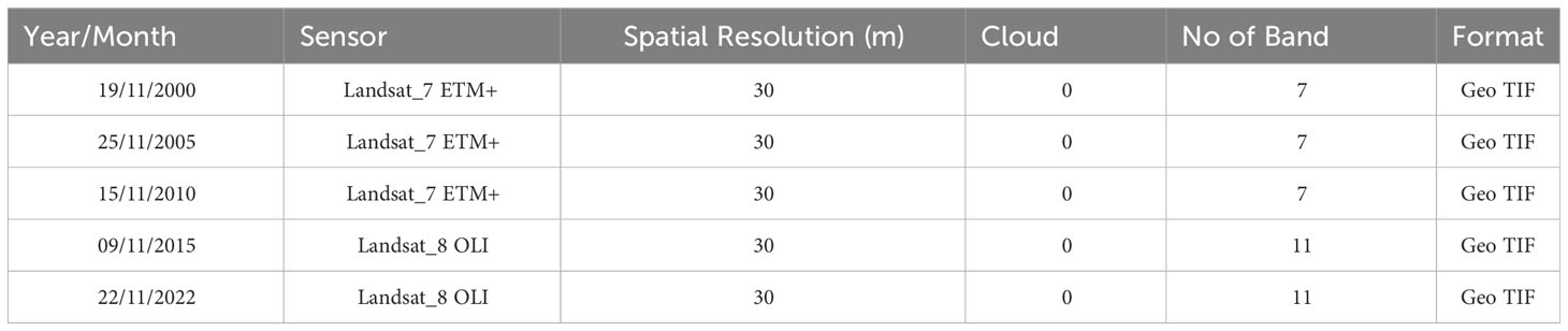
Table 1 details information of the dataset.

2.2 Water and non-water attributes are separated using a spectral index

The typical approach for detecting surface water changes involves isolating water features from multi-dated satellite images before conducting comparisons to identify alterations (Xu, 2006; Xu et al., 2010; El-Asmar and Hereher, 2011; Zhou et al., 2011; Du et al., 2012). Feyisa et al. (2014), the automatic water extraction index (AWEI) has been proposed for mapping water bodies. The AWEI index is applied for shoreline extraction, but it is emphasized in studies that the AWEI method cannot extract small areas of water. MNDWI is simple but efficient and user-friendly and performs well in shoreline extraction, according to Wang and ve ark (2017) suggested. Within the scope of this study, Landsat images have been examined to detect shoreline changes. An analysis of shoreline changes in the selected areas was conducted using the Digital Shoreline Analysis System (DSAS). DSAS is a statistical tool designed for studying shoreline changes, and it provides valuable insights into coastal environmental dynamics (Sheeja and Ajay Gokul, 2016; Thieler et al., 2017; Selamat et al., 2019). The user-friendly interface developed for DSAS enhances users’ ability to access valuable information, facilitating the generation of interactive reports for analysis (Moussaid et al., 2015; Abdul Maulud et al., 2022). In this study, multi-temporal LANDSAT imagery was employed and an appropriate index was selected that encompasses common bands from both the ETM and OLI sensors. Specifically, the Near-Infrared and Green bands, which are shared by Landsat 7 and 8 sensors were focused on. Consequently, McFeeters’ NDWI was adopted (Normalized Difference Water Index) as it is recommended for describing water features due to its superior accuracy compared to other indices, especially when manually and theoretically adjusted thresholds are taken into account (Das and Pal, 2017). To calculate NDWI, Equation 1 was used as proposed by McFeeters (1996), where GreenBOA and NIRBOA represent the reflectance of the green and Near-Infrared bands, respectively. The NDWI values range from -1 to 1. Typically, NDWI yields positive results for water features and negative results for non-water features (McFeeters, 1996). Our goal was to demarcate the coastline by distinguishing between water and non-water features. This was accomplished through binary image classification, in which values were assigned to each of the images: 0 to non-water features and 1 to water features, as outlined by (Das and Pal, 2017). For a visual representation, please refer to Figure 2A.

Figure 2

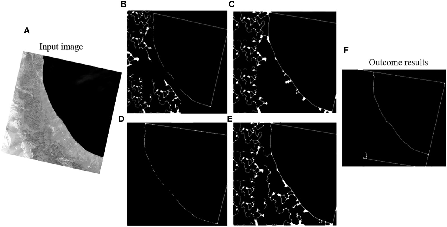
Figure 2 To showcase the results of the automatic coastline extraction, (A) The input includes the original image or NDWI. (B) The outcome of coastline extraction using the Prewitt technique. (C) The outcome of coastline extraction using the Sobel technique. (D) The outcome of coastline extraction using the Robert technique. (E) The outcome of coastline extraction using the Log technique. (F) The outcome of coastline extraction using our proposed Canny technique.

$\begin{array}{ll}\mathrm{NDWI}=\frac{\text{Gree}{n}_{BOA}-NI{R}_{BOA}}{Gree{n}_{BOA}+NI{R}_{\text{BOA}}}& (1)\end{array}$

2.3 Coastline extraction

Various techniques for edge detection are available for the extraction of shorelines from RS imagery. These techniques include common operators such as Sobel, Canny, Prewitt, and Robert. These algorithms are renowned for their simplicity and speed in detection. In our study, we specifically chose the Canny Edge algorithm for the automatic extraction of precise coastlines, eliminating the labor-intensive process of manual digitization. The Canny technique, rooted in optimization principles, effectively addresses the limitations of other gradient operators. It is widely recognized as the most successful and commonly employed grayscale edge detection technique. The objective of this study was to conduct an in-depth analysis of RS image edge detection, adhering closely to the procedural steps outlined in the Canny technique. As a result, it was noticed that the Canny edge detection operator emerges as the most effective choice for obtaining welldefined image edges with remarkable continuity and minimal breakpoints. In satellite images, the boundaries between sea and land exhibit a step-like edge transformation as the image’s grayscale values shift from land to seawater. This characteristic aligns with the precision of the Canny operator in edge positioning. When contrast to other techniques, Canny excels in accurately delineating coastal lines within a limited time and iterations. The extraction process is finalized during the detection step of this method. The Canny technique comprises four primary steps in its implementation, as outlined in Canny’s work from 1986 (Canny, 1986).

• To reduce noise in the image, a Gaussian function G(x, y) is employed to convolve the image f(x, y), resulting in a smoother image g(x, y) as described by Equations 2, 3.

$\begin{array}{ll}G(x,y)=\frac{1}{\sqrt{2\pi \alpha }}\exp (\frac{-(x^2+y^2}{2{\alpha }^2})& (2)\end{array}$

$\begin{array}{ll}g(x,y)=f(x,y)*G(x,y)& (3)\end{array}$

• Calculate the gradient direction and amplitude by employing a suitable gradient operator to assess the size and direction of the gradient for each pixel in the noise-reduced image.

• Utilize the non-maximum suppression (NMS) technique to accurately pinpoint the positions of edge points. This involves comparing the gradient amplitudes of neighboring pixels. Pixels with higher amplitude values are identified as edge points of interest, while those with lower amplitudes are considered non-edge points.

• Proceed to detect edges with high and low thresholds after the initial processing. The edges obtained in the previous steps are typically rough, and it is necessary to distinguish between genuine and false edge points. Points below the low threshold are excluded, while those above the high threshold are designated as edge points. Points with intermediate strength are marked as weak points, and the algorithm assesses whether these weak edges are connected to the primary edge points. If a connection is established, the point is recorded as an edge point.

Following the completion of the coastline extraction step by MATLAB R2021b, the ArcGIS 10.5 version software conversion tool was used to convert the raster data into a vector format (Figures 2A–F). This allowed to obtain coastline shapefiles for each year of the study period. DSAS was then utilized to analyze changes in the coastline for Oman during the period 2000-2022. As depicted in Figure 3, the accuracy graph illustrates the relationship between time consumption and the precision of data provided by various coastline extraction techniques. Notably, Canny outperforms others with an impressive accuracy rate of 87.79%. This result affirms the efficacy of the proposed model for the extraction and identification of coastal lines.

Figure 3

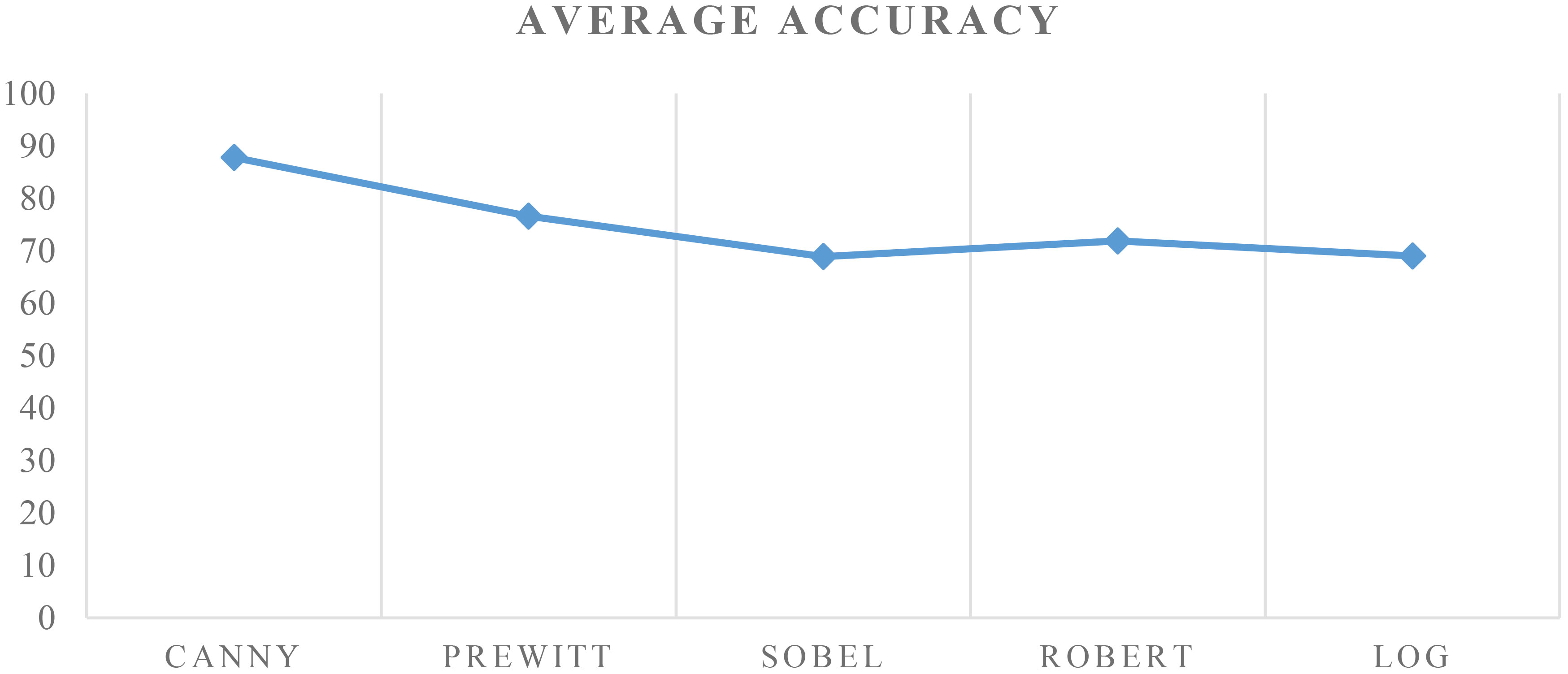
Figure 3 The extraction accuracy of different methods.

2.4 Interpretation and calculation of change rates

This research used statistical methods delivered by the DSAS application, designed to seamlessly integrate with the ESRI ArcGIS software, to calculate shoreline change rates. To achieve edge extraction, we followed the procedural steps outlined in the Canny technique to conduct a thorough analysis of RS image edge detection. Specifically, for our study, we utilized DSAS software version 5, developed by the US Geological Survey (Himmelstoss et al., 2018). Our approach involved the generation of orthogonal transects spaced 100 meters apart along the northeast coast of Oman using DSAS. The shoreline change statistics were calculated using three methods: End Point Rate (EPR), Linear Regression Rate (LRR), and Net Shoreline Movement (NSM). The EPR method was applied to monitor changes between successive coastline pairs, specifically for the years 2000-2005, 2005-2010, 2010-2015, and 2015-2022 (Figure 4).

Figure 4

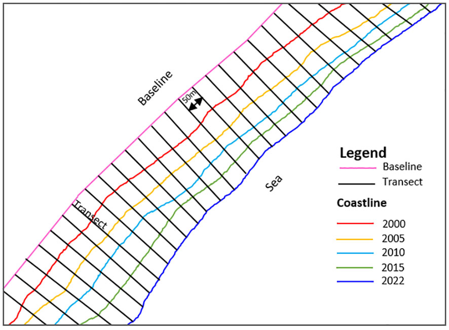
Figure 4 Shoreline with transect line.

In contrast, LRR statistics, which encompassed all shoreline data, were utilized to assess coastline variation over the entire 22-year from 2000 to 2022. The NSM method quantified the total distance of shoreline change between two specific periods. While LRR is commonly used to monitor shoreline dynamics (Crowell et al., 1991), it does not capture short-term trends that may occur between two successive periods due to various factors. The EPR statistic, on the other hand, illuminates these short-term trends for all transects between the four pairs of years. These change rates represent alterations in shoreline positions between two consecutive years, divided by the time elapsed between the two dates of coastline assessment. In our study, the time elapsed between shoreline pairs was typically five years, except for the final period, which spanned seven years.

3 Results and discussion

3.1 Coastline dynamic during the studied period

To conduct an extensive analysis of shoreline position changes spanning from 2000 to 2022, LRR technique was employed. This approach assesses the rate of change by fitting a least square regression to all shoreline positions, beginning with the oldest and progressing to the newest, along each of the transects. The results, as depicted in Figure 5, provide a comprehensive overview of global trends in shoreline change rates calculated using the LRR statistic. Positive values in this representation indicate shoreline accretion, while negative values signify coastal erosion. Additionally, Figure 5 offers insights into the specific locations of both accretion and erosion areas.

Figure 5

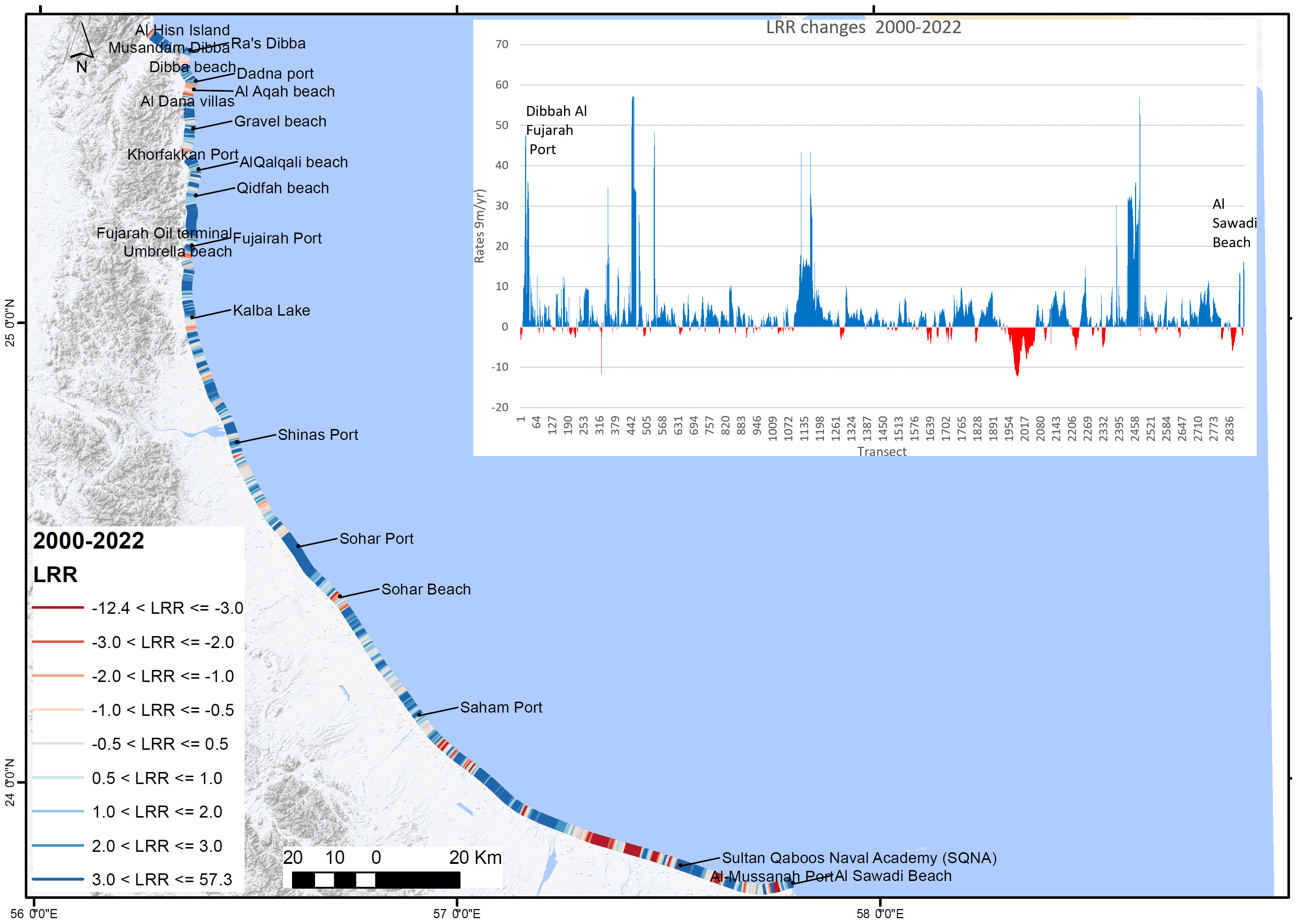
Figure 5 The long-term shoreline change rate from 2000 to 2022 was calculated using LRR. In the representation, transects with negative values (depicted in red) indicate erosion, while positive values (shown in blue) represent accretion rates.

The figure illustrates the computed long-term shoreline change rates using the Local Regression Rate (LRR) method for the period spanning 2000 to 2022. Each transect is color-coded, with negative values depicted in red, indicating erosion, and positive values shown in blue, representing accretion rates. The visual representation provides a clear spatial understanding of the coastal dynamics, allowing for the identification of areas experiencing erosion and accretion along the Oman coastline.

During the 22-year study period, both the overall average rates obtained through LRR and NSM analysis consistently indicated a prevailing trend of shoreline accretion. The average rate for LRR was 3.17 meters per year, while NSM showed an average distance of 77 meters. The long-term analysis results further underscored the dominance of accretion along the coastline, with 76.53% of transects exhibiting accretional behavior. Among these, 22.4% were statistically significant. In contrast, 23.47% of transects showed erosion, with only 1.24% of them having statistically significant erosion values. The maximum positive distance in NSM, signifying accretion, reached 1220.8 meters, while the maximum accretion rate based on LRR statistics was 57.28 meters per year. Notably, these maximum values were often associated with port infrastructure developments. EPR analysis results for the same period also confirmed the prevalence of the accretion process, with 82.36% of transects exhibiting accretion tendencies, and 51.64% of them being statistically significant. Conversely, 17.6% of transects showed erosion, and only 4.7% of these displayed statistically significant erosion. This period of observation witnessed notable fluctuations in shoreline dynamics, including both accretion and erosion trends. Remarkably, the areas of coastline undergoing significant changes were often characterized by intensive socio-economic activities, particularly urbanization, as evident in Figure 6. These findings strongly suggest that anthropogenic factors play a pivotal role in driving high shoreline changes along this coast. Figure 6 provides an illustrative representation of the dynamic changes in the littoral zone of Oman spanning the years 2000 to 2022. Extracted from Google Earth Pro, the illustration offers a detailed visual insight into the evolving coastal landscape, highlighting the impact of anthropogenic activities over this time-period. The distinctive features captured in the image include alterations in land cover, shoreline shifts, and the imprint of human interventions along the coastline. The comprehensive nature of this illustration serves to complement our findings, providing a tangible and accessible representation of the complex interactions between natural processes and anthropogenic influences in the studied region.

Figure 6

Figure 6 Visual representation of Oman’s littoral zone changes and anthropogenic activities from 2000 to 2022, extracted from Google Earth Pro. This figure succinctly captures the dynamic evolution of the coastline, highlighting the impact of human activities. High-resolution imagery provides key insights into the complex interplay between natural processes and anthropogenic influences.

3.2 Coastline change analysis

3.2.1 End point rate analysis

The short-term analysis reveals spatiotemporal trends and fluctuations in shoreline dynamics, enabling monitoring of the various stages of infrastructure development along this human-altered coastline. The Employment-Population Ratio (EPR) serves as a straightforward and effective method for assessing the evolution between two consecutive shoreline dates. Figure 7 presents the outcome of the EPR for different pairs of years, highlighting areas of significant accretion or erosion. These results also indicate variations in spatiotemporal change rate trends across different time periods.

Figure 7

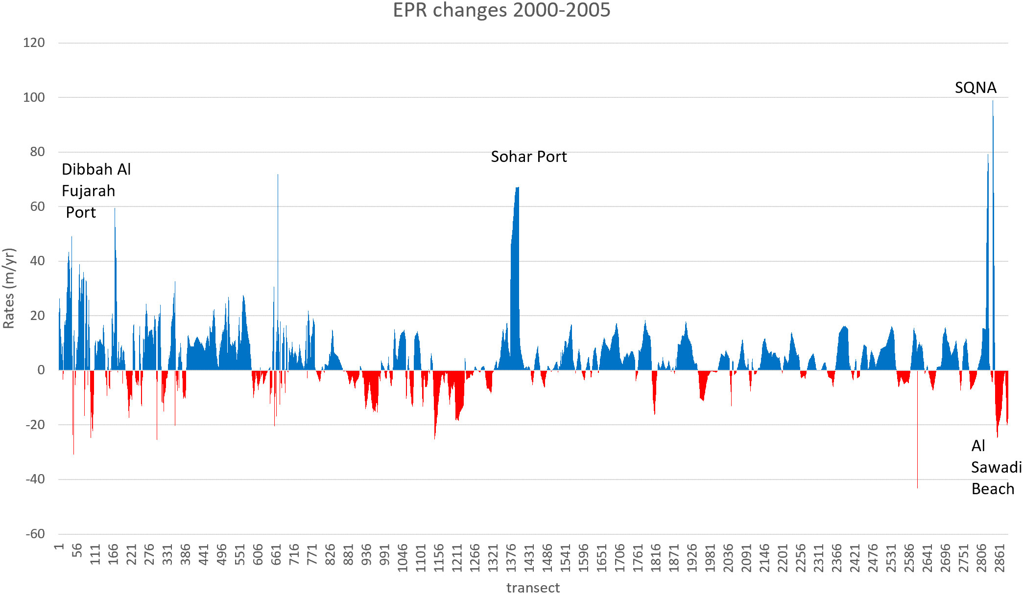
Figure 7 Displaying EPR changes from 2000 to 2005, where red signifies erosion and blue indicates accretion. This visual representation vividly illustrates the dynamic coastal alterations during this specific timeframe, offering a clear distinction between areas experiencing erosion (in red) and those undergoing accretion (in blue).

3.2.2 Shoreline changes 2000-2005

Figure 7 illustrates the rates of coastline position changes calculated using the EPR technique for this specific time period. The statistical analysis reveals that the Oman coastline primarily experiences accretion, with an average rate of 4.58 m/yr. More specifically, 66.45% of all transects exhibit accretion, with 29.44% of them displaying statistically significant accretion. In contrast, 33.55% of all transects show erosion, and only 7.23% of these exhibit statistically significant erosion. The maximum recorded accretion rate reached 99.07 m/yr, while the maximum erosional rate stands at -43.16 m/yr. Notably, this period is marked by significant sections with notably high erosion rates, with the highest values, both in terms of erosion and accretion, located in the southern part of the coastline.

Figure 7 presents a detailed visualization of EPR (Erosion and Accretion) changes along the Oman coastal zone during the period 2000-2005. Transects are color-coded to indicate the nature of change, with red representing erosion and blue denoting accretion. The visual analysis offers a snapshot of the dynamic coastal processes, highlighting regions experiencing erosion in red and areas undergoing accretion in blue. This color-coded mapping provides a clear and concise representation of the evolving coastal landscape during the specified timeframe, contributing valuable insights into the directional changes and potential areas of concern.

3.2.3 Shoreline changes 2005-2010

During this period, significant fluctuations between progradation and erosion were observed, as computed using the EPR techniques (see Figure 8). Notably, this timeframe is characterized by the highest rates of both accretion and erosion. These trends align with the patterns observed in previous periods. The average rate stands at 4.26 m/yr, with 54.13% of all transects showing accretion, and 25.59% of them exhibiting statistically significant accretion rates. Additionally, 45.87% of the transects experience erosion and 13.39% of these display statistically significant erosion. The maximum accretion rate, reaching 184.7 m/yr, is found in the Sohar Port area.

Figure 8

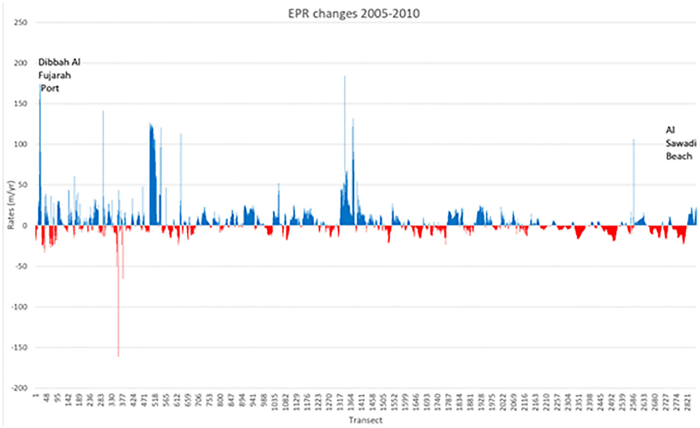
Figure 8 Illustrating EPR changes from 2005 to 2010, with red denoting erosion and blue representing accretion. This visual depiction provides a clear differentiation between areas experiencing coastal erosion (depicted in red) and those undergoing accretion (depicted in blue) during the specified timeframe.

3.2.4 Coastline changes 2010-2015

The EPR statistics for this period are graphically presented in Figure 9, highlighting that both eroded and prograded sections of the shoreline exhibit approximately equal rates of change. The average rate stands at 0.25 meters per year, with 50.35% of all transects demonstrating accretion, and 19.1% of them displaying statistically significant accretion. On the other hand, 49.65% of all transects experience erosion, and 14.89% of these exhibit statistically significant erosion. The maximum accretion rate reaches 126.93 meters per year, while the maximum erosion rate plunges to -177.03 meters per year. These peak values are concentrated in the southern part of the coastal area.

Figure 9

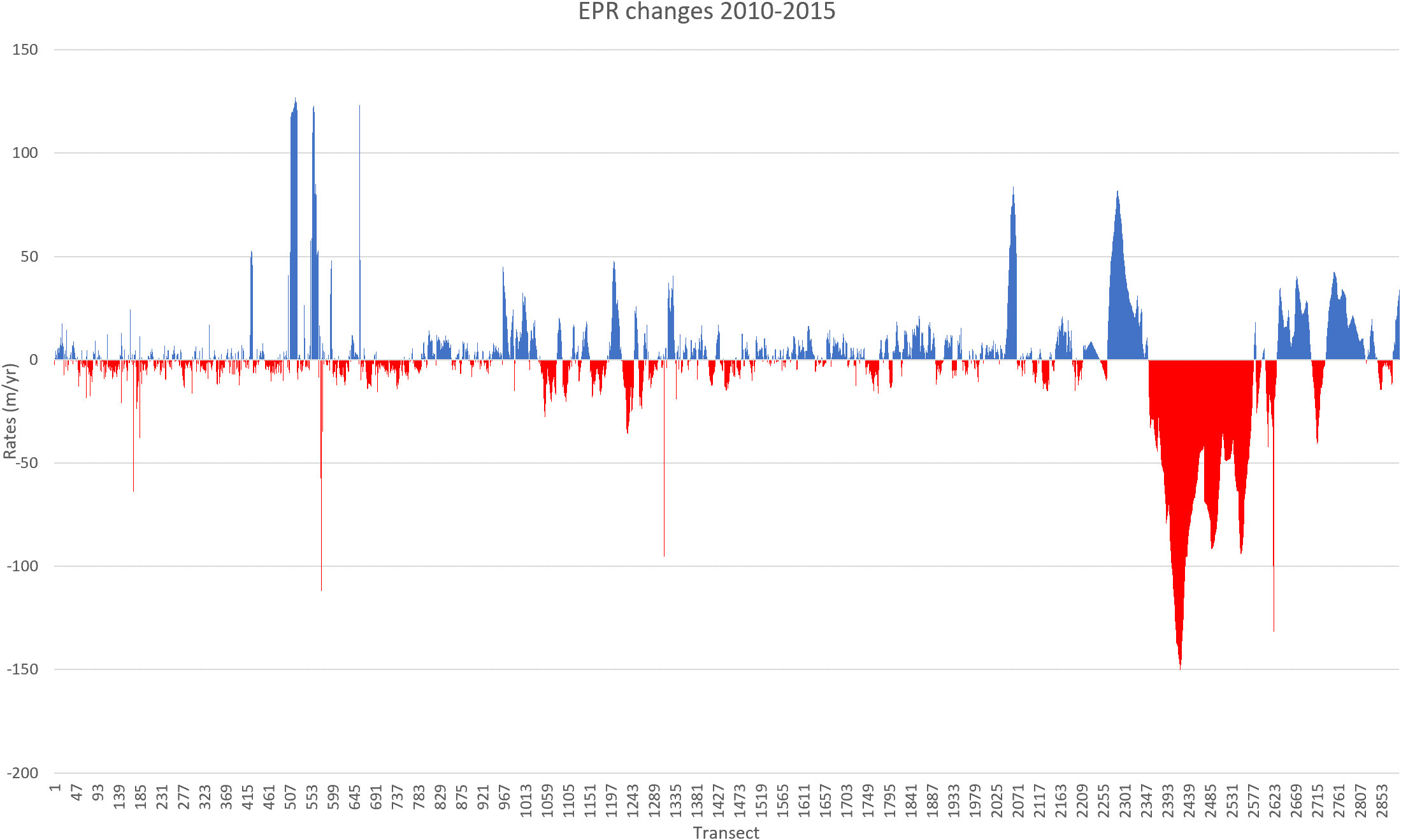
Figure 9 Visualizing EPR changes from 2010 to 2015, where red indicates erosion and blue signifies accretion. This graphical representation offers a clear distinction between areas experiencing coastal erosion (depicted in red) and those undergoing accretion (depicted in blue) during the specified timeframe.

3.2.5 Shoreline changes 2015-2022

The EPR statistics for the final period, as depicted in Figure 10, reveal a progradation trend, with an average rate of 5.27 meters per year. Specifically, 58.1% of all transects show accretion and 29.9% of them exhibit statistically significant accretion. In contrast, 41.9% of the transects experience erosion. The highest accretion value, 130.6 meters per year, is located in the Dibba Al Fujairah port area, while the maximum erosion rate reaches -53.2 meters per year.

Figure 10

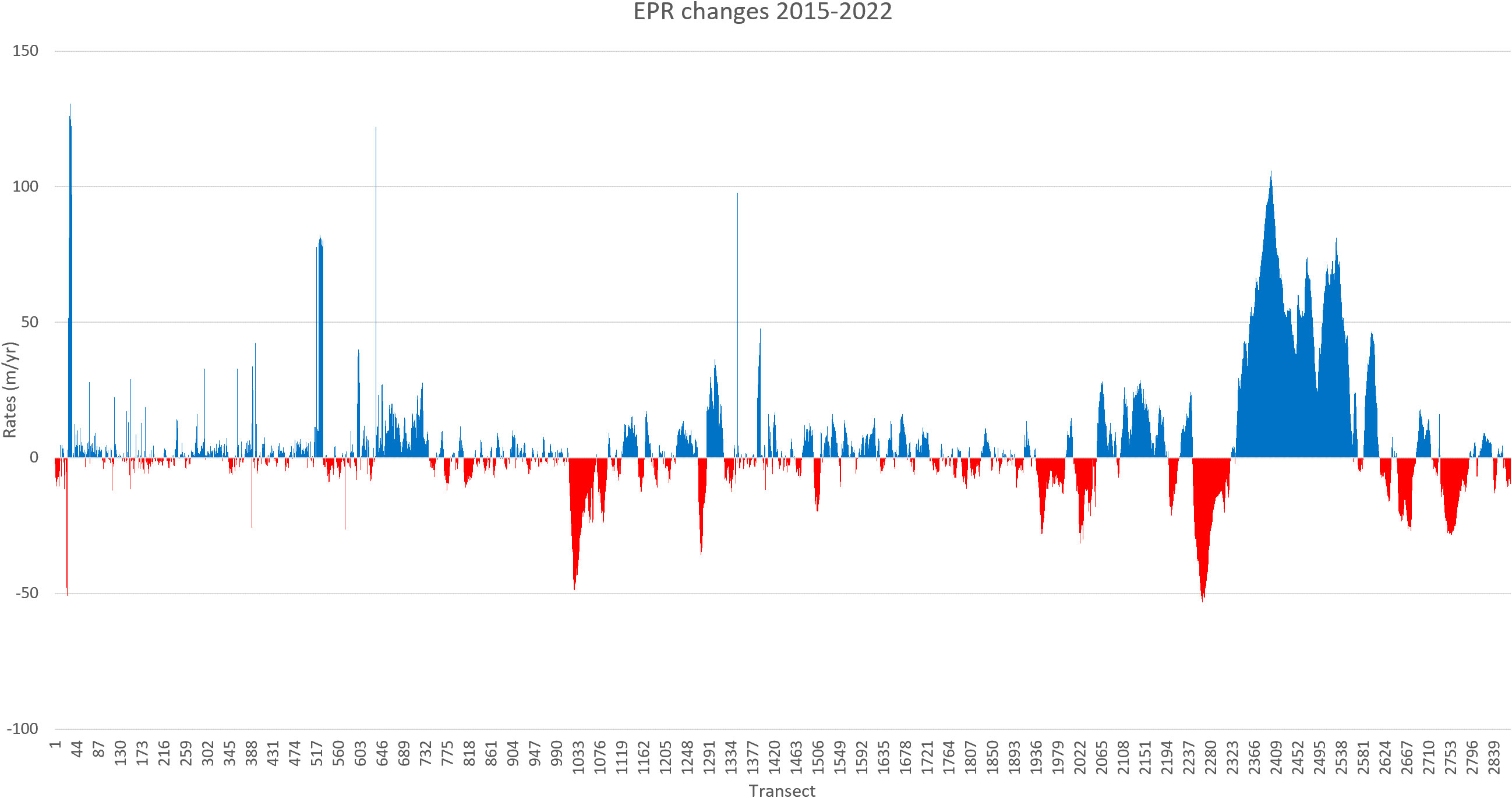
Figure 10 Displaying EPR changes from 2015 to 2022, with red indicating erosion and blue representing accretion. This visual representation delineates areas experiencing coastal erosion (in red) and those undergoing accretion (in blue) during the specified timeframe.

3.3 Land loss and land gain

The Oman shoreline has changed over time due to processes of both accretion and erosion. However, it’s important to note that the entire coastline has predominantly experienced accretion, with erosion occurring but to a lesser extent throughout the entire period. Between 2000 and 2022, the most significant accretion took place (Figure 11). The coastal regions have predominantly witnessed extensive socioeconomic activities and urbanization, with a notable emphasis on the proliferation of large port infrastructure. Long-term spatiotemporal assessments of coastline changes, spanning from 2000 to 2022, underscore the significant influence of anthropogenic activities on shoreline dynamics. The most significant alterations involve land progradation toward the sea, a transformation primarily driven by human interventions. Conversely, certain sections of the shoreline have experienced erosion, primarily attributed to human pressures. A closer examination of these rates over time reveals a growing anthropogenic footprint and urban expansion along the coast.

Figure 11

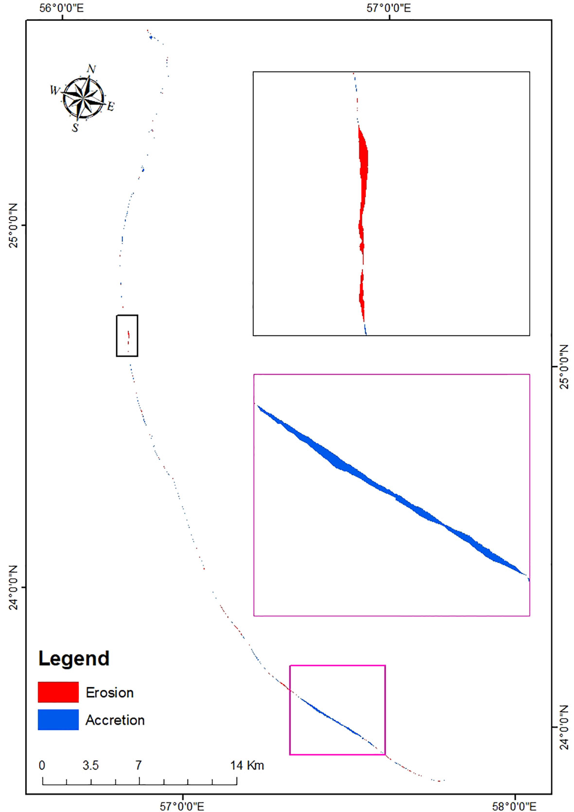
Figure 11 Map illustrating land loss and gain along the Oman coastline from 2000 to 2022. This visual representation provides a comprehensive overview of the dynamic changes in coastal areas, highlighting regions experiencing land loss and those undergoing land gain over the examined period.

Continuous monitoring of shoreline changes highlights that, across all time periods, seaport areas and their neighboring regions have consistently expanded seaward. These shifts in coastline shape have far-reaching implications for the coastal environment, impacting ecosystems, marine habitats, and benthic communities in the near-shore area. Additionally, industrial cities in the vicinity may pose pollution challenges as a result of these changes.

4 Ecological & socio-economic Implications

4.1 Ecological implications

Our research delves into the ecological consequences of changes observed in the Oman coastline. Landsat images have allowed us to assess changes in land cover, vegetation, and coastal features. The implications for local ecosystems are multifaceted, encompassing potential impacts on biodiversity, habitat loss, and changes in coastal dynamics. Our findings contribute valuable insights into the vulnerability of coastal ecosystems to various anthropogenic and natural factors. changes in coastal dynamics, such as erosion and accretion, can disrupt the delicate balance of sediment transport and coastal geomorphology. This not only affects the stability of coastal ecosystems but also alters nutrient cycling, sediment deposition patterns, and shoreline protection mechanisms. Consequently, the resilience of coastal ecosystems to natural disturbances and climate change-induced stressors may be compromised, exacerbating the risk of biodiversity loss and ecosystem degradation.

4.2 Socio-economic implications

The socio-economic implications of coastal changes are crucial for understanding the broader impacts on communities and industries. Our study explores the interactions between coastal transformations and local socio-economic activities, such as fisheries, tourism, and infrastructure development. Our objective is to provide stakeholders and policymakers with a comprehensive understanding of the potential impacts of these changes on livelihoods, resource utilization, and community resilience by analyzing these connections. The livelihoods of coastal communities are intricately linked to the health and stability of coastal ecosystems. For instance, changes in coastal morphology and habitat degradation can significantly impact fisheries productivity, jeopardizing the livelihoods of fisherfolk reliant on marine resources for sustenance and income. Similarly, the tourism sector, which thrives on pristine coastlines and marine attractions, may suffer adverse consequences from coastal erosion and degradation, leading to economic losses and employment uncertainties for local communities dependent on tourism-related activities. Moreover, coastal infrastructure, including ports, harbors, and residential settlements, is vulnerable to the impacts of coastal erosion and sea-level rise. The degradation of coastal defenses and inundation of coastal areas pose substantial risks to infrastructure integrity, public safety, and property values, necessitating costly adaptation and mitigation measures. The socio-economic ramifications of these challenges extend beyond immediate economic losses to encompass broader issues of community resilience, social cohesion, and equitable access to resources.

4.3 Policy and management recommendations

To address the identified ecological and socio-economic implications, our research includes recommendations for sustainable coastal management and policy considerations. Our findings will be incorporated into future planning initiatives in order to help develop strategies that balance economic development with ecological conservation and promote long-term well-being.

In summary, our study not only focuses on the technical aspects of image extraction and change analysis but also aims to provide a holistic understanding of the broader consequences for the environment and society. The opportunity to emphasize the ecological and socio-economic dimensions of our work is greatly appreciated, and we believe that this comprehensive approach enhances the significance and applicability of our research.

5 Conclusion

In the present research, we conducted a spatiotemporal assessment of coastline variations along the Oman coast, utilizing GIS and RS technologies. Utilizing the DSAS application and multitemporal satellite data, we analyzed 22 years of data concerning the coastline of Oman. Canny-based edge extraction was used in this study to automatically delineate the study area, resulting in more precise and finer representations of the coastline. Clearly, accretion has been observed along the coast of Oman. To gain a detailed understanding of these changes, the LRR method proved advantageous. However, the EPR method proved effective when the coastline exhibited either consistent seaward or landward movement. Statistical techniques, such as EPR, NSM, and LRR were used to quantify the rates of coastline change that allows the user to evaluate both long-term and short term trends. Study identified areas of significant accretion and erosion between 2000 and 2022. Assessing spatiotemporal coastline variations in a non-structural manner presents a feasible alternative for coastal area management. Additionally, this study contributes to understanding coastline susceptibility. Over the past 22 years, human activities have exerted a more significant influence on coastal topography than natural factors, with artificial structures dominating the natural shoreline. Moreover, research emphasizes the critical role of coastline alterations as a primary physical influence. Continued monitoring of areas prone to land loss is crucial, considering their significance for future tourism and urban planning.

Data availability statement

The raw data supporting the conclusions of this article will be made available by the authors, without undue reservation.

Ethics statement

The paper does not deal with any ethical problems.

Author contributions

AC: Conceptualization, Data curation, Formal analysis, Funding acquisition, Investigation, Methodology, Project administration, Resources, Software, Supervision, Validation, Visualization, Writing – original draft, Writing – review & editing.

Funding

The author(s) declare that financial support was received for the research, authorship, and/or publication of this article. This paper was supported by the International Maritime College Oman Internal Grant Project.

Conflict of interest

The authors declares that the research was conducted in the absence of any commercial or financial relationships that could be construed as a potential conflict of interest.

The reviewer HM declared a past collaboration with the author to the handling editor.

Publisher’s note

All claims expressed in this article are solely those of the authors and do not necessarily represent those of their affiliated organizations, or those of the publisher, the editors and the reviewers. Any product that may be evaluated in this article, or claim that may be made by its manufacturer, is not guaranteed or endorsed by the publisher.

References

Abdul Maulud K. N., Selamat S. N., Mohd F. A., Md Noor N., Wan Mohd Jaafar W. S., Kamarudin M. K. A., et al. (2022). Assessment of shoreline.

Google Scholar

Abushandi E., Abualkishik A. (2020). Shoreline erosion assessment modelling for Sohar Region: Measurements, analysis, and scenario. Sci. Rep. 10 (1), 4048.

PubMed Abstract | Google Scholar

Adebola A. O., Ojoye S., Ibitoye M. O. (2017). Geospatial Analysis of Coastal Land Use/Land cover Pattern and Shoreline Changes in Akwa-Ibom State, Nigeria.

Google Scholar

Alesheikh A. A., Ghorbanali A., ve Talebzadeh A. (2004). “Generation the Coastline Change Map for Urnia Lake by TM and ETM+ Imagery,” in Map Asia 2004(Beijing).

Google Scholar

Al-Hatrushi S., Ramadan E., Charabi Y. (2015). Application of geo-processing model for a quantitative assessment of coastal exposure and sensitivity to sea level rise in the Sultanate of Oman. Am. J. Climate Change 4 (04), 379.

Google Scholar

Apostolopoulos D., Nikolakopoulos K. (2021). A review and meta-analysis of remote sensing data, GIS methods, materials and indices used for monitoring the coastline evolution over the last twenty years. Eur. J. Remote Sens. 54, 240–265. doi: 10.1080/22797254.2021.1904293.

CrossRef Full Text | Google Scholar

Apostolopoulos D. N., Avramidis P., Nikolakopoulos K. G. (2022). Estimating quantitative morphometric parameters and spatiotemporal evolution of the Prokopos Lagoon using remote sensing techniques. J. Mar. Sci. Eng. 10 (7), 931.

Google Scholar

Baig M. R. I., Ahmad I. A., Shahfahad, Tayyab M., Rahman A. (2020). Analysis of shoreline changes in Vishakhapatnam coastal tract of Andhra Pradesh, India: an application of digital shoreline analysis system (DSAS). Ann. GIS 26, 361–376. doi: 10.1080/19475683.2020.1815839.

CrossRef Full Text | Google Scholar

Boak H., Turner I. L. (2005). Shoreline definition and detection. A Rev. J. Coast. Res., 688–703. doi: 10.2112/03-0071.1.

CrossRef Full Text | Google Scholar

Canny J. (1986). A computational approach to edge detection. IEEE Trans. Pattern Anal. Mach. Intell. PAMI-8 (6), 679–698. doi: 10.1109/TPAMI.1986.4767851.

CrossRef Full Text | Google Scholar

Cracknell A. P. (1999). Remote sensing techniques in estuaries and coastal zones—An update. Int. J. Of Remote Sens. 19, 485–496.

Google Scholar

Crowell M., Leatherman S. P., Buckley M. K. (1991). Historical shoreline change: error analysis and mapping accuracy. J. Coast. Res., 839–852.

Google Scholar

Dasgupta S., Laplante B., Meisner C., Wheeler D., Yan J. (2009). The impact of sea level rise on developing countries: a comparative analysis. Climatic Change 93 (3-4), 379–388.

Google Scholar

Das R. T., Pal S. (2017). Exploring geospatial changes of wetland in different hydrological paradigms using water presence frequency approach in Barind Tract of West Bengal. Spatial Inf. Res. 25, 467–479. doi: 10.1007/s41324-017-0114-6.

CrossRef Full Text | Google Scholar

Dolan R., Hayden B. P., May P., May S. K. (1980). There liability of shoreline change measurements from aerial photographs. Shore and Beach 48, 22–29.

Google Scholar

Du Z., Linghu B., Ling F., Li W., Tian W., Wang H., et al. (2012). Estimating surface water area changes using time-series Landsat data in the qingjiang river basin, China. J. Appl. Remote Sens. doi: 10.1117/1.JRS.6.063609.

CrossRef Full Text | Google Scholar

El-Asmar H. M., Hereher M. E. (2011). Change detection of the coastal zone east of the Nile Delta using remote sensing. Environ. Earth Sci. 62, 769–777. doi: 10.1007/s12665-010-0564-9.

CrossRef Full Text | Google Scholar

Eliot I., Clarke D. (1989). Temporal and spatial bias in the estimation of shoreline rate-of-change statistics from beach survey information. Coast. Manage. 17, 129–156.

Google Scholar

Feyisa G. L., Meilby H., Fensholt R., Proud S. R. (2014). Automated water extraction index: A new technique for surface water mapping using landsat imagery. Remote Sens. Environ. 140, 23–35. doi: 10.1016/j.rse.2013.08.029

CrossRef Full Text | Google Scholar

Gazioğlu C., Burak S., Alpar B., Türkerd A., Barutc I. F. (2010). Foreseeable impacts of sea level rise on the southern coast of the marmara sea (Turkey). Water Policy 12, 932–943. doi: 10.2166/wp.2010.050.

CrossRef Full Text | Google Scholar

Ghaderi D., Rahbani M. (2020). Detecting shoreline change employing remote sensing images (Case study: Beris Port-east of Chabahar, Iran). Int. J. Of Coastal Offshore And Environ. Eng. 5, 1–8.

Google Scholar

Gurel M. (2018). Determination of shoreline change by satellite images: Sinop province sample (Aksaray: Yuksek Lisans Tezi, Aksaray Üniversitesi Fen Bilimleri Enstitüsü / Harita Mühendisliği Ana Bilim Dalı).

Google Scholar

Hanson H., Gravens M. B., Kraus N. C. (1988). “Prototype applications of A generalized shoreline change numerical model,” in Proceedings Of The 21st International Conference On Coastal Engineering, Costa del Sol-Malaga, Spain. 1265–1279.

Google Scholar

Himmelstoss E. A., Henderson R. E., Kratzmann M. G., Farris A. S. (2018). Digital shoreline analysis system (DSAS) version 5.0 user guide (US Geological Survey), 2331–1258.

Google Scholar

Hossain Md S., Yasir M., Wang P., Ullah S., Jahan M., Hui S., et al. (2021). Automatic shoreline extraction and change detection: A study on the southeast coast of Bangladesh. Mar. geology 441, 106628. doi: 10.1016/j.margeo.2021.106628.

CrossRef Full Text | Google Scholar

Hui S., Mengliang G., Yuliang G., Mingming X., Shanwei L., Yasir M., et al. (2022). Coastline extraction based on multi-scale segmentation and multi-level inheritance classification. Front. Mar. Sci. 9, 1031417. doi: 10.3389/fmars.2022.1031417.

CrossRef Full Text | Google Scholar

Jensen J. R. (1996). Introductory digital image processing: a remote sensing perspective (Prentice-Hall Inc).

Google Scholar

Kevin W., El Asmar H. M. (1999). Monitoring changing position of coastlines using thematic mapper imagery, an example from the Nile Delta. Geomorphology 29, 93–105. doi: 10.1016/S0169-555X(99)00008-2.

CrossRef Full Text | Google Scholar

Kuleli T., Guneroglu A., Karsli F., Dihkan M. (2011). Automatic detection of shoreline change on coastal Ramsar wetlands of Turkey. Ocean Eng. 38 (10), 1141–1149.

Google Scholar

Kwarteng A. Y., Al-Hatrushi S. M., Illenberger W. K., McLachlan A., Sana A., Al-Buloushi A. S., et al. (2016). Beach erosion along Al Batinah coast, Sultanate of Oman. Arabian J. Geosciences 9 1-20.

Google Scholar

Kwarteng A. Y., Dorvlo A. S., Vijaya Kumar G.T. (2009). Analysis of a 27-year rainfall dat–2003) in the Sultanate of Oman. Int. J. Climatology: A J. R. Meteorological Soc. 29 (4), 605–617.

Google Scholar

Leatherman S. P. (2001). Social and economic costs of sea-level rise. Sea-level rise, History and Consequences. Eds. Douglas B. C., Kearney M. S., Leatherman S. P. (Academic Press), 181–223. doi: 10.1016/S0074-6142(01)80011-5.

CrossRef Full Text | Google Scholar

Li X., Michiel C. J. (2010). Damen Coastline change detection with satellite remote sensing for environmental management of the Pearl River Estuary, China. J. Mar. Syst. 82, S54–S61.

Google Scholar

Lotfy I. (2012). Prestressed concrete wind turbine supporting system.

Google Scholar

McFeeters S. K. (1996). The use of the Normalized Difference Water Index (NDWI) in the delineation of open water features. Int. J. Remote Sens. 17, 1425–1432. doi: 10.1080/01431169608948714.

CrossRef Full Text | Google Scholar

Morton R. A., Speed F. M. (1998). Evaluation of shorelines and legal boundaries controlled by water levels on sandy beaches. J. Coast. Res. 144, 1373–1384.

Google Scholar

Moussaid J., Ait Flora A., Zourarah B., Maanan M. (2015). Using automatic computation to analyze the rate of shoreline change on the Kenitra coast, Morocco. Ocean. Eng. 102, 71–77. doi: 10.1016/j.oceaneng.2015.04.044.

CrossRef Full Text | Google Scholar

Mullick M. R. A., Islam K. A., Tanim A. H. (2020). Shoreline change assessment using geospatial tools: a study on the Ganges deltaic coast of Bangladesh. Earth Sci. Inf. 13, 299–316. doi: 10.1007/s12145-019-00423-x.

CrossRef Full Text | Google Scholar

Nahiduzzaman K. M., Aldosary A. S., Rahman M. T. (2015). Flood induced vulnerability in strategic plan making process of Riyadh city. Habitat Int. 49, 375–385. doi: 10.1016/j.habitatint.2015.05.034.

CrossRef Full Text | Google Scholar

Nidhinarangkoon P., Ritphring S., Kino K., Oki T. (2023). Shoreline changes from erosion and sea level rise with coastal management in phuket, Thailand. J. Mar. Sci. Eng. 11, 969. doi: 10.3390/jmse11050969.

CrossRef Full Text | Google Scholar

Pandey A., Singh K., Sharma A. (2023). Integrating NDWI, MNDWI, and Erosion Modeling to Analyze Wetland Changes and Impacts of Land Use Activities in Ropar Wetland (India).

Google Scholar

Parthasarathy K. S. S., Deka P. C. (2019). Remote sensing and GIS application in assessment of coastal vulnerability and shoreline changes. Changes for the Selangor Coast, Malaysia, Using the Digital Shoreline Analysis System Technique. Urban Sci. 6, 71. doi: 10.3390/urbansci6040071

CrossRef Full Text | Google Scholar

Rahman M. K., Crawford T. W., Islam M. S. (2022). Shoreline change analysis along rivers and deltas: A systematic review and bibliometric analysis of the shoreline study literature from 2000 to 2021. Geosciences 12, 410. doi: 10.3390/geosciences12110410.

CrossRef Full Text | Google Scholar

Seilheimer T. S., Wei A., Chow-Fraser P., Eyles N. (2007). Impact of urbanization on the water quality, fish habitat, and fish community of a Lake Ontario marsh, Frenchman’s Bay. Urban Ecosyst. 10, 299–319. doi: 10.1007/s11252-007-0028-5.

CrossRef Full Text | Google Scholar

Selamat S. N., Maulud K. N. A., Mohd F. A., Rahman A. A. A., Zainal M. K., Wahid M. A. A., et al. (2019). Multi method analysifor identifying the shoreline erosion during northeast monsoon season. J. Sustain. Sci. Manage. 14, 43–54.

Google Scholar

Shaghude Y. W., Wannäs K. O., Lundén B. (2003). Assessment of shoreline changes in the western side of Zanzibar channel using satellite remotesensing. Int. J. Remote Sens. 24, 4953–4967.

Google Scholar

Sheeja P. S., Ajay Gokul A. J. (2016). Application of digital shoreline analysis system in coastal erosion assessment. Int. J. Eng. Sci. Comput. 6, 7876–7883.

Google Scholar

Smith A. W. S., Jackson L. A. (1992). The variability in width of the visible beach. Shore Beach 602, 7–14.

Google Scholar

Thieler E. R., Himmelstoss E. A., Zichichi J. L., Ergul A. (2017). The Digital Shoreline Analysis System (DSAS), Version 4.0 (Reston, VA, USA: U.S. Geological Survey).

Google Scholar

Uçkaç Ş. (1998). “Kıyı Alanlarında Coğrafi Bilgi Sistemlerinin Kullanımı,” in Türkiye’ nin Kıyı ve Deniz Alanları 2. Ulusal Konferansı, 22-25 Eylül 1998, Ankara, Türkiye Kıyıları 98 Konferansı Bildiriler Kitabı, 557–564.

Google Scholar

Wang Z., ve ark (2017). Spatio-Temporal change detection of ningbo coastline water 2017 9, 816.

Google Scholar

Xu H. (2006). Modification of normalized difference water index (NDWI) to enhance open water features in remotely sensed imagery. Int. J. Remote Sens. 27, 3025–3033.

Google Scholar

Xu Y. B., Lai X. J., Zhou C. G. (2010). Water surface change detection and analysis of bottomland submersion-emersion of wetlands in Poyang Lake reserve using ENVISAT ASAR data. China Environ. Sci. 30, 57–63.

Google Scholar

Yasir M., Hui S., Binghu H., Rahman S. U. (2020a). Coastline extraction and land use change analysis using remote sensing (RS) and geographic information system (GIS) technology–A review of the literature. Rev. Environ. Health 35, 453–460. doi: 10.1515/reveh-2019-0103.

PubMed Abstract | CrossRef Full Text | Google Scholar

Yasir M., Hui S., Hongxia Z., Hossain M. S., Fan H., Zhang L., et al. (2021). A spatiotemporal change detection analysis of coastline data in qingdao, east China. Sci. Programming 2021, 1–10. doi: 10.1155/2021/6632450.

CrossRef Full Text | Google Scholar

Yasir M., Liu S., Mingming X., Wan J., Pirasteh S., Dang K. B. (2024). ShipGeoNet: SAR image-based geometric feature extraction of ships using convolutional neural networks. IEEE Trans. Geosci. Remote Sensing. doi: 10.1109/TGRS.2024.3352150.

CrossRef Full Text | Google Scholar

Yasir M., Sheng H., Fan H., Nazir S., Niang A. J., Salauddin M., et al. (2020b). Automatic coastline extraction and changes analysis using remote sensing and GIS technology. IEEE Access 8, 180156–180170. doi: 10.1109/Access.6287639.

CrossRef Full Text | Google Scholar

Zheng H., Li X., Wan J., Xu M., Liu S., Yasir M. (2023). Automatic coastline extraction based on the improved instantaneous waterline extraction method and correction criteria using SAR imagery. Sustainability 15, 7199. doi: 10.3390/su15097199.

CrossRef Full Text | Google Scholar

Zhou H., Hong J., Huang Q. (2011). Landscape and water quality change detection in urban wetland: A post-classification comparison method with IKONOS data. Proc. Environ. Sci. 10, 1726–1731. doi: 10.1016/j.proenv.2011.09.271.

CrossRef Full Text | Google Scholar