HyFish: hydrological factor fusion for prediction of fishing effort distribution with VMS dataset

Predicting fishing effort distribution is crucial for guiding fisheries management in developing effective strategies and protecting marine ecosystems. This task requires a deep understanding of how various hydrological factors, such as water temperature, surface height, salinity, and currents influence fishing activities. However, there are significant challenges in designing the prediction model. Firstly, how hydrological factors affect fishing effort distributions remains unquantified. Secondly, the prediction model must effectively integrate the spatial and temporal dynamics of fishing behaviors, a task that shows analytical difficulties. In this study, we first quantify the correlation between hydrological factor fields and fishing effort distributions through spatiotemporal analysis. Building on the insights from this analysis, we develop a deep-learning model designed to forecast the daily distribution of fishing effort for the upcoming week. The proposed model incorporates residual networks to extract features from both the fishing effort distribution and the hydrological factor fields, thus addressing the spatial limits of fishing activity. It also employs Long Short-Term Memory (LSTM) networks to manage the temporal dynamics of fishing activity. Furthermore, an attention mechanism is included to capture the importance of various hydrological factors. We apply the approach to the VMS dataset from 1,899 trawling fishing vessels in the East China Sea from September 2015 to May 2017. The dataset from September 2015 to May 2016 is used for correlation analysis and training the prediction model, while the dataset from September 2016 to May 2017 is employed to evaluate the prediction accuracy. The prediction error ratio for each day of the upcoming week range is only 5.6% across all weeks from September 2016 to May 2017. HyFish, notable for its low prediction error ratio, will serve as a versatile tool in fisheries management for developing sustainable practices and in fisheries research for providing quantitative insights into fishing resource dynamics and assessing ecological risks related to fishing activities.

1 Introduction

The oceans are currently experiencing a critical ecological deterioration, with an alarming number of species facing the risk of extinction (Bongaarts, 2019). This crisis can be attributed, in part, to the extensive and unsustainable fishing practices that have significantly depleted fishery resources, resulting in adverse effects on marine ecosystems and biodiversity (Demirel et al., 2023). To promote sustainable development, it is imperative for fishery management authorities to analyze the dynamic changes in fishing activities promptly y. By utilizing the spatiotemporal distribution of fishing effort, they can assess the impacts of these activities on fish species and the marine environment (Rijnsdorp et al., 1998; Kaiser et al., 2000; Stefansson and Rosenberg, 2005), and develop evidence-based fishery management policies (Dinmore et al., 2003; Jin et al., 2021). In this context, the quantitative analysis and prediction of fishing effort distribution play a pivotal role in providing valuable insights and guidance for sustainable fisheries management.

Previous research on fishing effort distribution can be broadly divided into two categories. The first kind of approaches involve statistical analysis of historical data, which focuses on studying the evolution and impact of fishing effort distribution, as well as the characteristics of fishing hotspots. The second kinds of approach involve predicting fishing effort distribution using mathematical models, machine learning, or deep learning techniques.

Statistical analyses in fisheries has largely focused on historical data analysis to discern patterns in fishing effort distribution. Vianna et al. (2020) noted a stable catch trend in the Marshall Islands from 1950 to 1990, followed by a decrease in catches despite increased effort in the 2000s. De la Puente et al. (2020) observed in Peruvian fisheries that fishing efforts grew faster than catches from 1950 to 2018, leading to unsustainable fishing practices. Russo et al. (2019) reported a yearly decline in Italian fishing efforts in the Mediterranean from 2006 to 2016. Li et al. (2021) identified high-effort fishing zones near the South China Sea coast, while Russo et al. (2020) studied the effects of maritime zone regulations on Adriatic Sea fishing patterns. These studies, however, do not predict future fishing effort distributions.

Recent advancements in fisheries research have seen a shift towards using mathematical models or artificial intelligence to predict fishing efforts. Chen et al. (2017) proposed an entry-fishing model based on Gaussian distributions that correlated the index of entry-fishing with sea surface temperature (SST) or sea surface temperature anomaly (SSTA). Cimino et al. (2019) crafted a system to forecast fishing activities within Palau’s exclusive economic zones, taking into account a range of oceanic and climatic variables, which helped identify periods of peak fishing. Yuan et al. (2021) developed a deep learning approach employing Convolutional Neural Networks (CNN) and Multi-layer Perceptron (MLP), enabling monthly predictions of fishing efforts in the Western and Central Pacific based on environmental factors and VMS data. Zhao et al. (2021) explored the use of deep learning to understand and predict weekly short-term fishing effort distributions, utilizing the chronology of fishing activities among trawlers. These diverse methodologies underscore the growing emphasis on predictive studies of fishing effort distributions.

While previous studies have made progress in predicting fishing effort distribution on a monthly or weekly scale, there is still a lack of prediction at the daily level for the upcoming week. Furthermore, the influence of marine hydrological factors, such as sea surface temperature, height, salinity, and ocean current on fish activity patterns have not been analyzed quantitatively. These factors play significant roles in shaping the distribution of fishing effort (Leitão, 2023). Although some research has considered hydrological factors in fishing effort distribution prediction, there is a lack of comprehensive analysis regarding the correlation between evolution in hydrological factors fields and fishing effort distributions. Additionally, suitable methods to effectively integrate hydrological factors into the prediction of fishing effort distribution have not been adequately designed, resulting in limited applicability of the coarse predictions.

Facing these limitations, this study introduces HyFish, a prediction system of day-level fishing effort distribution for the upcoming week that incorporates historical VMS and hydrological factors datasets. The ability to predict fishing effort distributions on a daily basis for the upcoming week will present a significant advancement in fisheries management. This granular level of prediction offers detailed insights into the evolving dynamics of fishing effort distributions. By providing day-to-day predictions, such intricacies as daily fluctuations, peak periods, and potential shifts in fishing patterns become discernible, offering a comprehensive understanding of fishing effort distributions over the upcoming week. More importantly, these daily predictions serve as a crucial tool for fishery administrations, furnishing them with timely alerts about changes in fishing activities. This immediacy allows for swift and effective management decisions, enabling authorities to regulate trawler activities on a much shorter timescale than previously possible. Such proactive governance not only aids in sustainable fishery management but also helps in mitigating overfishing and preserving marine ecosystems, ensuring a balanced approach between exploitation and conservation. To achieve accurate prediction, HyFish has to express three kinds of constraints in its prediction model.

 (1) Hydrological factor constraints: It needs to quantify and represent the influence of key hydrological factors, including sea surface temperature, height, salinity, and ocean current, on fish effort distribution. Furthermore, it may take different delays for the evolution of different kinds of hydrological factors affecting the fishing effort distribution.

 (2) Spatial constraints: The fishing behavior exhibits both proximity and remote characteristics. Proximity refers to fishing vessels engaging in continuous fishing activities in adjacent areas. Conversely, the remote characteristic describes the phenomenon where fishing vessels travel significant distances after fishing in one area and subsequently resume fishing in distant areas.

 (3) Temporal constraints: The fishing activities of vessels display periodicity patterns. The fishing habits of fishermen are traditionally formed under tidal conditions. Therefore, the fishing activities also exhibit a periodic pattern.

HyFish is structured into two primary components to address the outlined constraints: the hydrological impact assessment and the prediction model. The first component uses spatiotemporal correlation analysis to measure the influence of each hydrological factor on fishing effort distribution and to determine the time lags associated with these factors, effectively addressing hydrological constraints and laying the groundwork for the prediction model.

The second component is divided into two modules: the Encoder and the Decoder. The Encoder, consisting of fusion blocks and an Long Short-Term Memory (LSTM) network, focuses on feature extraction. It processes historical data of fishing effort distributions along with hydrological factor fields. The fusion blocks, employing deep residual networks, extract latent features from these inputs, with convolution operations handling spatial constraints. Attention mechanisms are integrated to evaluate the relevance of various hydrological factors in predicting fishing effort distribution. The LSTM network then discerns the temporal relationships within the fused features daily and outputs these hidden features.

The Decoder, also based on LSTM, is responsible for the day-by-day prediction of the forthcoming week’s fishing effort distribution. It utilizes the hidden features produced by the Encoder and the current fishing effort distribution as inputs. Trained on the dataset from September 2015 to May 2016, the model exhibits a daily prediction error ratio between 5.0% and 6.2%, with an overall average error ratio of 6.0% across all weeks from September 2016 to May 2017.

The main contributions can be summarized as follows:

 (1) We have developed a day-level fishing effort distribution system for the next week, called HyFish, which fuses VMS data and hydrological factor field sequences. The system incorporates a well-designed deep learning network to accurately predict fishing effort distribution.

 (2) We have quantified the impact of evolving hydrological factor fields on fishing effort distribution through spatiotemporal correlation analysis and calculated the delays in impact for different hydrological factors. We have quantified the impact of evolving hydrological factor fields on fishing effort distribution through spatiotemporal correlation analysis and calculated the delays in impact for different hydrological factors.

 (3) Extensive experiments demonstrate that HyFish achieves high accuracy in day-level prediction of fishing effort distribution for the upcoming week.

2 Data and methods

2.1 Data

The study utilizes a VMS dataset collected from 1,899 otter trawlers between September 2015 and May 2017. This dataset covers the fishing areas of Zhoushan and Yushan in the East China Sea, extending to additional zones within the coordinates of 120°-130°E and 25°-35°N. The VMS data, which tracks the trajectory of active fishing vessels, was compiled by the Zhejiang Oceanic and Fishery Bureau, China. Data acquisition was done through the BeiDou Satellite System, recording at a three-minute interval. Each VMS entry includes key details such as vessel identification, timestamp, longitude, latitude, speed, and course.

For analysis, the fishing areas are divided into spatial cells, each with a resolution of 0.1° × 0.1°. The fishing effort data are aggregated daily. We filter out the fishing records using the threshold method proposed in (Hong et al., 2019). These records, representing three-minute intervals of fishing effort, are then allocated to the corresponding grid and date. Thus, for any given date, we calculated the fishing effort distribution, with the unit of measurement for each grid being in minutes.

Moreover, the study incorporates a hydrological factor dataset sourced from the Copernicus Climate Data Store. The hydrological factors analyzed include sea surface height (SSH), sea surface temperature (SST), sea surface salinity (SSS), and ocean current (Current). The specific Copernicus products utilized are SEALEVEL_EUR_PHY_L4_MY_008_068 for SSH and Current, MULTIOBS_GLO_PHY_S_SURFACE_MYNRT_015_013 for SSS, and GLOBAL_MULTIYEAR_PHY_001_030 for SST. Each of these datasets features a spatial resolution of 0.125° × 0.125° and a daily temporal resolution, with data structured in a grid-like format.

The geographical focus for both the VMS and hydrological factor datasets is within the coordinates of 120°E-130°E and 25°N-35°N, ensuring consistency in the study area. The sizes of the VMS and hydrological factor datasets are approximately 18.90 GB and 7.39 GB, respectively.

Given that the fishing cessation period for otter trawlers is from June to August, we divided the two datasets into non-overlapping train and test datasets. The train dataset spans September 1, 2015 to May 30, 2016, while the test dataset spans September 1, 2016 to May 31, 2017. The train dataset is used to quantify the impact of the evolution of marine hydrological factor fields on fishing effort distribution and to train the prediction model. The test dataset will evaluate the prediction accuracy of HyFish.

2.2 Methods

This section provides an in-depth exploration of the design details. We begin by providing definitions for key terms employed in the paper and formulating the prediction problem. Then we analyze the correlation between the evolution of hydrological factor field and fishing effort distribution. Lastly, we provide the comprehensive design of the prediction model.

2.2.1 Problem statement

We first introduce the basic notations utilized in the paper and then formulate the prediction problem.

2.2.1.1 Fishing effort Distribution

Given a day τ, assume that $X_{\tau }\in {ℝ}_{+}^{I\times J}$ is a fishing effort distribution partitioned evenly into I ×J grids, where a gird (i,j) is considered as a spatial region of 0.1°× 0.1° and each item $X_{\tau }^{(i,j)}\in {ℝ}_{+}$ denotes the fishing effort of this grid on day τ. The historical fishing effort distribution sequence for P days till day τ can be represented as $X_{\tau -P+1,\tau }\in {ℝ}_{+}^{P\times I\times J}$.

2.2.1.2 Hydrological factor fields

Marine hydrological factor fields of SSH, SST, SSS and Current on day τ are defined as $H_{\tau },T_{\tau },S_{\tau },C_{\tau }$, respectively. For example, $S_{\tau }^{(i,j)}\in {ℝ}_{+}$ denotes the SSS value in grid (i,j) on day τ, The historical SSS sequence for a duration of P days till day τ can be represented as $S_{\tau -P+1,\tau }\in {ℝ}_{+}^{P\times I\times J}$. We use M_τ to represent the combination of all hydrological factor fields. i.e. $M_{\tau }=(H_{\tau },T_{\tau },S_{\tau },C_{\tau })$.

2.2.1.3 Impact lag

The aggregation of fish stock will be influenced by evolution in marine hydrological factor fields, which in turn indirectly impacts the fishing effort distributions. However, the impact of marine hydrological factor fields on fishing effort distribution may have different delays, called impact lag, denoted by $d_H^{*},d_T^{*},d_S^{*},d_C^{*}$ for SSH, SST, SSS and Current, respectively. We use d^∗ to label the impact lags for all hydrological factor fields. i.e. $d^{*}=d_H^{*},d_T^{*},d_S^{*},d_C^{*}$.

2.2.1.4 Problem statement

Take the historical fishing effort distribution sequence X_τ−P+1,τ and marine hydrological factor fields sequences $M_{\tau -d^{\ast }-P+1,\tau -d^{\ast }}=(H_{\tau -d_H^{\ast }-P+1,\tau -d_H^{\ast }},T_{\tau -d_T^{\ast }-P+1,\tau -d_T^{\ast }},S_{\tau -d_S^{\ast }-P+1,\tau -d_S^{\ast }},C_{\tau -d_C^{\ast }-P+1,\tau -d_C^{\ast }})$ as inputs, we construct the prediction model F in Equation 1 to predict the future fishing effort distribution sequence. ${\widehat{X}}_{\tau }+1,\tau +L$ for L days.

$\begin{array}{ll}\begin{array}{l}{\widehat{X}}_{\tau +1,\tau +L}=F_{\Theta }(X_{\tau -P+1,\tau },H_{\tau -d_H^{*}-P+1,\tau -d_H^{*}},T_{\tau -d_T^{*}-P+1,\tau -d_T^{*}},\\ S_{\tau -d_S^{*}-P+1,\tau -d_S^{*}},C_{\tau -d_C^{*}-P+1,\tau -d_C^{*}})\end{array}& (1)\end{array}$

Θ denotes all the learnable parameters of the prediction model. The choices of P and L will be discussed later in this section.

2.2.2 Hydrological impact quantification

The impact lag represents the delayed effect of evolution in marine hydrological factor fields on the evolution of fishing effort distribution. To determine the impact lag, it is crucial to understand the relationship between the evolution in marine hydrologic factor fields and the fishing effort distribution.

To quantify this relationship, we first conduct a correlation analysis in the temporal dimension, calculating the relationship under different impact delays for each spatial grid. Then, we focus on the spatial dimension and select an optimal impact delay across all the grids for each hydrological factor.

Let’s take the impact of the Sea Surface Salinity (SSS) on the fishing effort distribution sequence for grid (i, j) as an example. We introduce our methods to calculate the correlation for this grid. Assuming that the train dataset contains N days, the correlation for different time lags d_s between the fishing effort distribution sequence on day τ and the corresponding previous salinity sequence can be calculated as Equation 2.

$\begin{array}{ll}CorrSS{S}_{\tau }^{(i,j)}(d_s)=\frac{Cov(X_{ \tau -P+1,\tau }^{(i,j)},S_{\tau -d_s-P+1,\tau -d_s}^{(i,j)})}{{\sigma }_{X_{ \tau -P+1,\tau }^{(i,j)}}{\sigma }_{S_{\tau -d_s-P+1,\tau -d_s}^{(i,j)}}}& (2)\end{array}$

P is the length of the sequence. Cov denotes the covariance operation, and σ denotes the standard deviation of a sequence. d_s is limited in the range of 0 to d^max.

After calculating for all spatial grids and all possible ds, we determine the optimal impact delay across all the spatial grids. We create a set of correlations and a set of strong correlations for all values of ds in Equations 3 and 4, respectively. A strong correlation is defined as a correlation value higher than 70%. The optimal impact delay is chosen as the value of ds which corresponds to the highest spatial ratio of strong correlation ρ as demonstrated in Equation 5. The operation ∥∥ is to calculate the size of the set.

$\begin{array}{ll}CorrSSS(d_s)=\left\{CorrSS{S}_{\tau }^{(i,j)}(d_s)|CorrSS{S}_{\tau }^{(i,j)}(d_s),for \tau \in (P,N),i\in [1,I],j\in [1,J]\right\}& (3)\end{array}$

$\begin{array}{ll}NCorrSSS(d_s)=\left\{CorrSSS(d_s)|CorrSSS(d_s)>0.7\right\}& (4)\end{array}$

$\begin{array}{ll}\rho =\frac{\Vert NCorrSSS(d_s)\Vert }{\Vert CorrSSS(d_s)\Vert },d_s^{*}={\text{max }}_{d_s}(\rho )& (5)\end{array}$

Since the delay in the impact of marine hydrological factors on fish aggregations is mostly about two weeks (Rubenstein, 2021), we set d^max = 14. The entire process of solving for $d_s^{\ast }$ is summarized in Algorithm 1. $d_H^{*},d_T^{*}$ and $d_C^{*}$ are calculated in the same way.

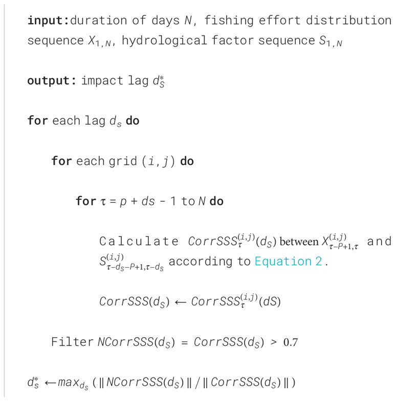
Algorithm 1. Hydrological impact quantification and impact lag calculation.

2.2.3 Model design

We propose a predictive model for forecasting the future fishing effort distribution sequence. Figure 1 presents the sketch of the model. The model follows a sequence-to-sequence structure (Britz et al., 2017) and comprises two primary components: Encoder and Decoder. The Encoder is first responsible for extracting spatial features from marine hydrological factor field sequence and fishing effort distribution sequence for each time step. It further utilizes LSTM (Long Short-Term Memory) (Gers et al., 2000) to learn the sequential features across the timeline. The Decoder, also employing LSTM, is responsible for generating predictions day-by-day the future fishing effort distribution over a specified period (L days). It takes the learned features from the Encoder and current fishing effort distribution as inputs to make predictions.

Figure 1

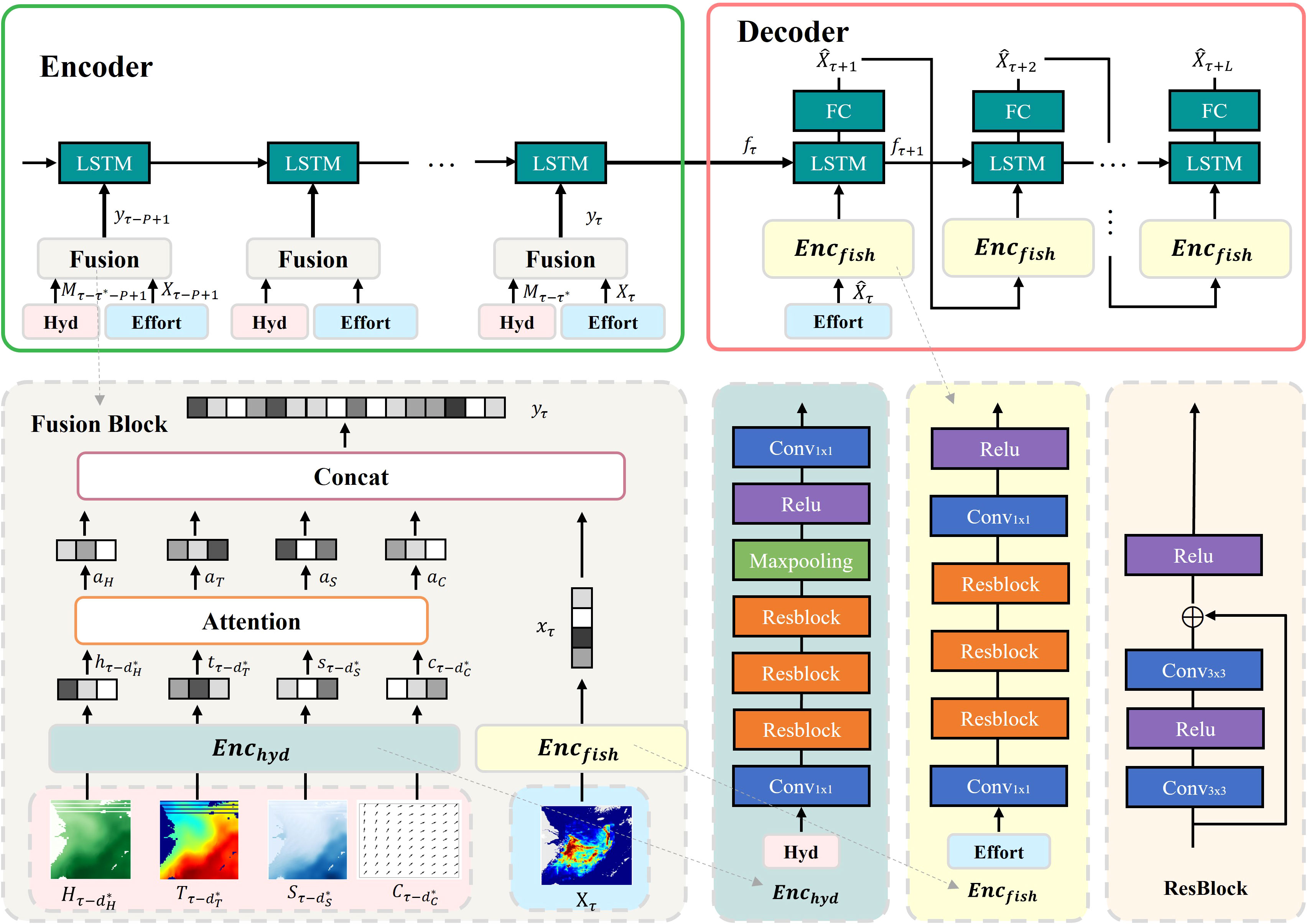
Figure 1 Sketch of the prediction model. The model is divided into two parts, Encoder and Decoder. The Encoder is responsible for extracting features from historical sequences, while the Decoder is responsible for making predictions. The Encoder consists of LSTM network and Fusion Blocks, with the Fusion Block expanded in the gray block in the bottom left corner. It extracts features from hydrological factor distributions through Enc_hyd and extracts features from fishing effort distributions through Enc_fish. The Decoder takes the current day’s fishing effort distribution as input, still utilizing Enc_fish to extract its features, and then makes daily predictions for the next week. Enc_hyd, Encoder for hydrological feature; Enc_fish, Encoder for VMS sequence’s features of trawlers.

2.2.3.1 Encoder

The historical fishing effort distribution sequence and hydrological factor sequence display clear spatiotemporal patterns. To effectively capture these patterns, the Encoder module is specifically designed to extract spatiotemporal features and fuse them.

The Encoder consists of two key components: LSTM and Fusion. The LSTM network serves as the backbone network, receiving spatial features extracted at each time step and capturing the temporal relationships among these steps. It generates encoded feature representations that guide the Decoder network. Fusion blocks are incorporated at each time step to extract features from both the fishing effort distribution sequence and the hydrological factor sequences with corresponding impact lags.

The Fusion block serves four functions. Firstly, it aims to extract fishing effort distribution features, capturing both local proximity and remote dependency. Local proximity refers to the tendency of nearby grids to have similar fishing effort distributions because vessels engage in continuous fishing activities across neighbor grids. On the other hand, remote dependency refers to the scenario where vessels steam to distant regions for subsequent fishing activities after fishing in one area. Although these locations may be geographically far apart, they are temporally adjacent in terms of fishing activities.

To capture the local spatial proximity in the fishing effort distribution, a convolutional neural network (CNN) with a 3x3 convolutional kernel is employed for feature extraction on fishing effort distribution. To address remote dependencies in fishing behavior, the CNN is stacked to enlarge the receptive field, enabling the establishment of correlations between grids that are far apart. Additionally, the inclusion of residual blocks helps overcome the issue of gradient vanishing or exploding that may arise from stacking multiple CNNs. The fishing effort distribution of each time step is projected into multiple channels, where each channel captures specific aspects or features via CNN. Subsequently, a Conv1x1 operation is applied to reduce the channel dimension to 1, further extracting features and the resulting feature is reshaped into a vector, denoted as x_τ. This process effectively extracts the spatial features from the fishing distribution X_τ for each time step τ. The whole step can be summarized as Equation 6.

$\begin{array}{ll}{x}_{\tau }=En{c}_{fish}(X_{\tau })& (6)\end{array}$

The second function of the Fusion block is hydrological feature extraction. Under different impact lags, the hydrological features extraction network is constructed with the residual blocks, which effectively capture the complex spatial patterns in the hydrological factors. For the given hydrological factor field input, $H_{\tau -d_H^{\ast }},T_{\tau -d_T^{\ast }},S_{\tau -d_S^{\ast }},C_{\tau -d_C^{\ast }}$, features extraction network is performed on each of these inputs individually. Similar to the fishing effort feature extraction, each input is projected into multiple channels with the first Con1x1 block. Subsequently, residual blocks are applied to extract high-level hydrological features. However, in contrast to the fishing effort feature extraction, a pooling layer is introduced to compress hydrological features. Finally, a Conv1x1 operation is employed to reduce the channel dimension to one, and then the output is reshaped into a one-dimensional vector, denoted as $h_{\tau -d_H^{\ast }},t_{\tau -d_T^{\ast }},s_{\tau -d_S^{\ast }}$ and $c_{\tau -d_C^{\ast }}$ respectively. This process allows for the extraction of spatial hydrological features from the input hydrological factor fields for each time step. The whole step can be summarized as Equation 7:

$\begin{array}{ll}{h}_{\tau -d_H^{*}},t_{\tau -d_T^{*}},s_{\tau -d_S^{*}},c_{\tau -d_C^{*}}=En{c}_{hyd}(H_{\tau -d_H^{*}},T_{\tau -d_T^{*}},S_{\tau -d_S^{*}},C_{\tau -d_C^{*}})& (7)\end{array}$

The third function of the Fusion block focuses on emphasizing the importance of different hydrological factors. Given that different hydrological factors have varying degrees of impact on fishing effort distribution, we introduce the attention mechanism to weight the importance of different hydrological factors in Equations 8, 9. W_k is a weight matrix and b_k is the bias terms of neurons. Both of them are learnable parameters.

$\begin{array}{ll}{z}_K=W_k^{T}tanh\left(W_k·k_{\tau -d_K^{*}}+b_k\right),k=\left\{h,t,s,c\right\},K=\left\{H,T,S,C\right\}& (8)\end{array}$

$\begin{array}{ll}{a}_K=\frac{exp(z_K)}{{\Sigma }_{K}exp(z_K)}& (9)\end{array}$

The last function is to combine the higher-level hydrological features and the higher-level fishing effort distribution feature through weighted concatenation using the learned parameters to obtain the fusion feature y_τ, as shown in Equation 10. The element-wise multiplication symbol $\otimes$ is used to denote the weighting process.

$\begin{array}{ll}{y}_{\tau }=concat \left(x_{\tau },h_{\tau -d_H^{*}}\otimes a_H,t_{\tau -d_T^{*}}\otimes a_T,s_{\tau -d_S^{*}}\otimes a_S,c_{\tau -d_C^{*}}\otimes a_C\right)& (10)\end{array}$

The LSTM component is designed to capture temporal relationships from the high-level fusion features along different time steps. LSTM is well-suited for processing sequential data due to its strong memory and modeling capabilities. The LSTM is modeled in Equation 11. f_τ denotes the output of LSTM.

$\begin{array}{ll}{f}_{\tau }=LSTM (y_{\tau -P+1},\dots ,y_{\tau -1},y_{\tau })& (11)\end{array}$

The entire encoder processes the historical fishing effort features along with the hydrological features and generates an output, which is transferred to the Decoder.

2.2.3.2 Decoder

The Decoder is designed to generate the fishing effort predictions for the future τ + 1 to τ + L days. It still utilizes LSTM as the core component. LSTM’s memory units allow it to retain and propagate previous states. This capability is crucial for generating coherent outputs, particularly when there are dependencies between different parts of the output sequence. The Decoder generates the prediction for the future L days using recursive ways. Specifically, it takes the hidden state f_τ from the Encoder’s output and the current fishing effort distribution X_τ as inputs. It generates the hidden state f_τ+1 and predict the fishing effort distribution on day $\tau +1,{\widehat{X}}_{\tau }+1$. Then it takes f_τ+1 and ${\widehat{X}}_{\tau }+1$ as inputs and generates f_τ+2 and ${\widehat{X}}_{\tau }+2$ for the subsequent day’s prediction. This recursive process allows the Decoder to predict fishing effort distribution for the future L days. The recursive prediction can be summarized as Equations 12, 13. Here f is the hidden state and the range of l is 1 to L.Enc_fish refers to the effort extraction module mentioned in the Encoder and FC refers to the full connected layer shown in Figure 1.

$\begin{array}{ll}{f}_{\tau +l}=LSTM \left(En{c}_{fish}\left({\widehat{X}}_{\tau +l-1}\right),f_{\tau +l-1}\right)& (12)\end{array}$

$\begin{array}{ll}{\widehat{X}}_{\tau +l}=FC(f_{\tau +l})& (13)\end{array}$

After designing the model, we choose the values of the model parameters, including the length of the input sequence (P), the number of residual blocks (b) in the feature extraction network of fishing effort distribution and hydrological factor, and the length of the output sequence (L).

To determine the value of P, we analyzed of the distribution of voyage durations for all vessels in the train and test dataset, as shown in Figure 2. We observe that approximately 90% of voyage durations are within two weeks. To ensure that the input contains most of the complete voyage, we set P to two weeks.

Figure 2

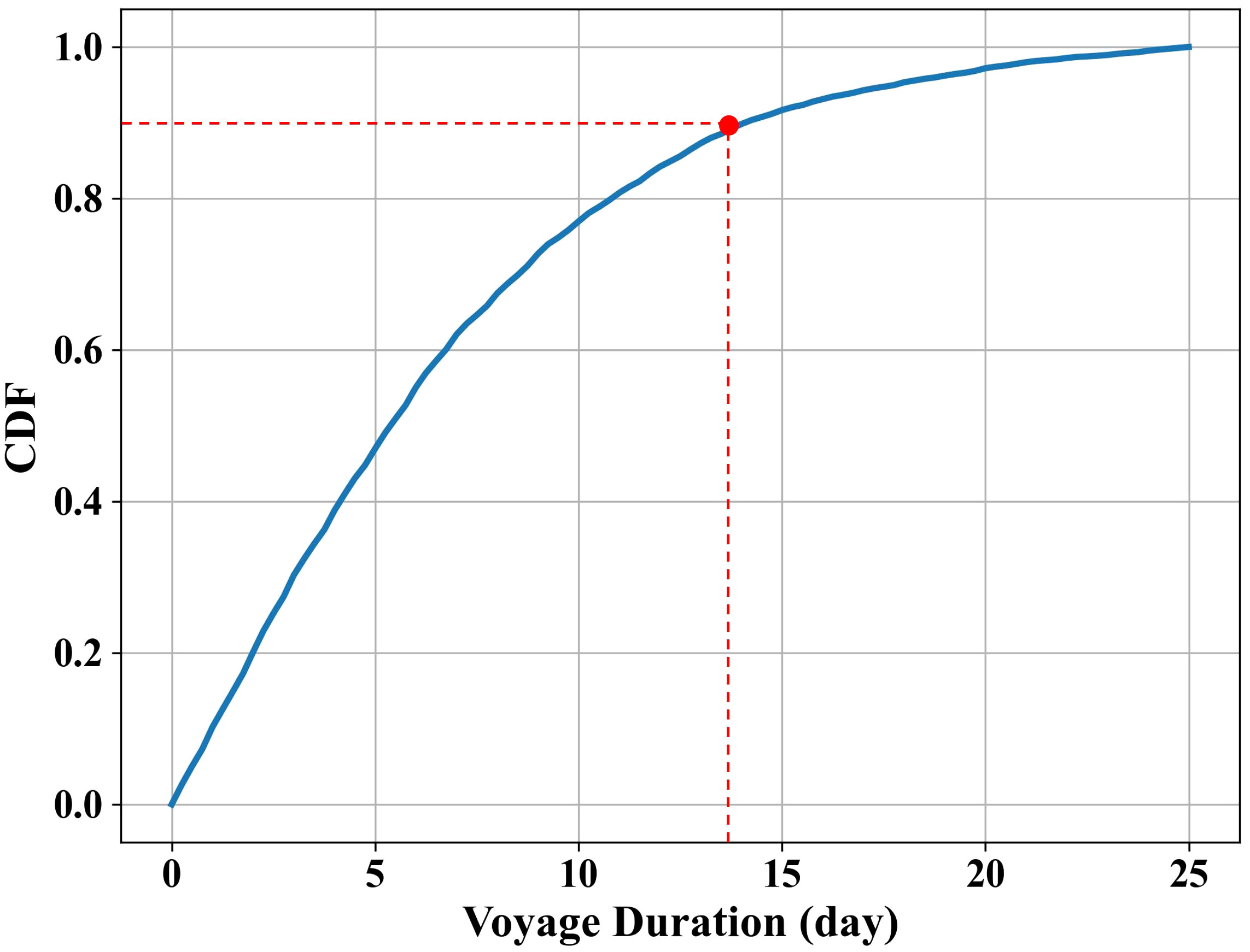
Figure 2 CDF (Cumulative Distribution Function) of voyage duration of all trawlers.

To determine the residual block number of the feature extraction network, we analyzed the distribution of the number of grids covered by a vessel in a single day’s operation, as shown in Figure 3. The analysis revealed that approximately 90% of vessels cover six or fewer grids in their daily voyages. Based on this observation, we set b as 3, which let the spatial perceptive field of 3 × 3 convolution operation cover six grids. This choice allows the model to capture the desired spatial region, as well as eliminating the impact of unrelated grids.

Figure 3

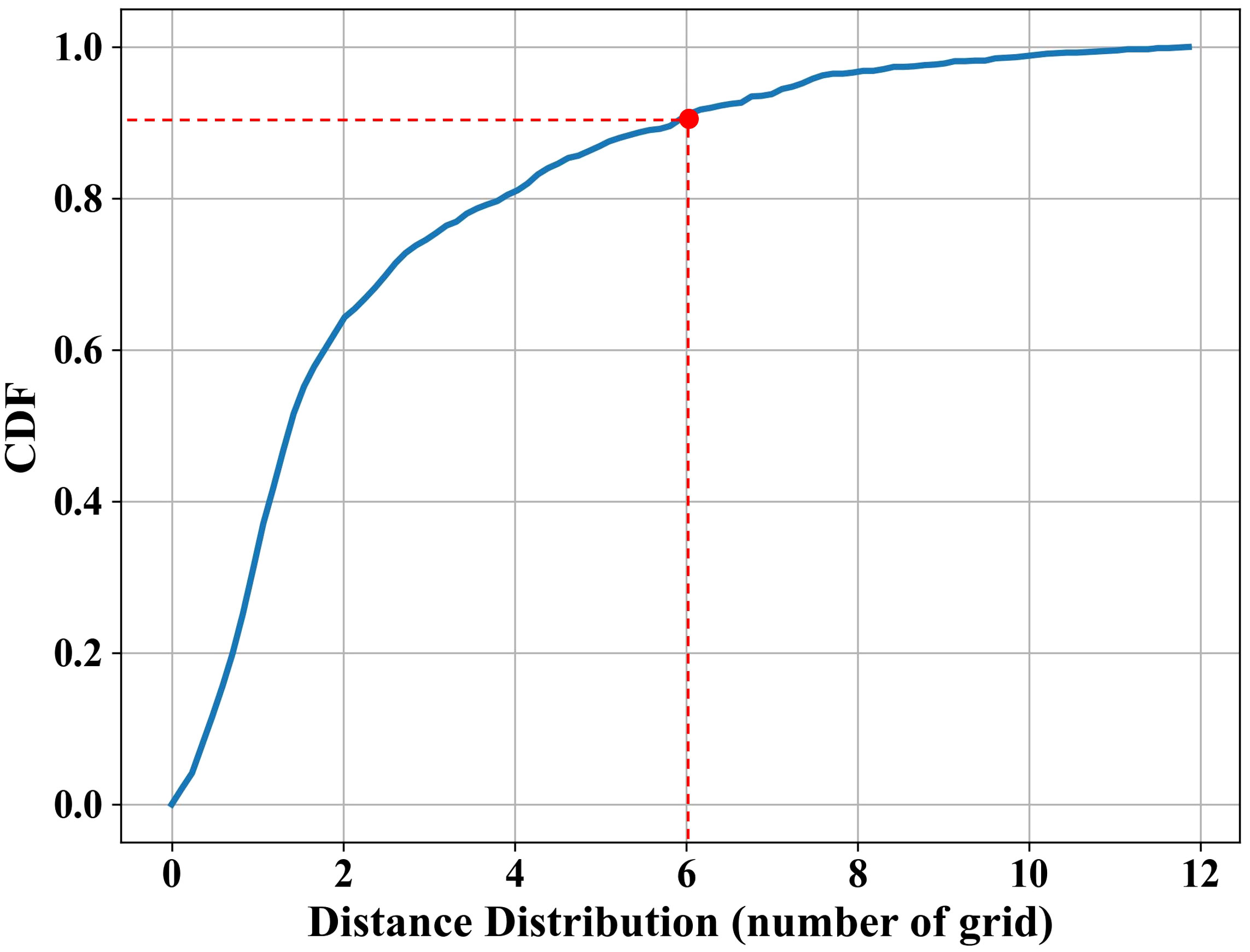
Figure 3 CDF of grid number trawlers span in a day.

To determine the value of L, we analyze the temporal patterns of fishing effort in hotspot grids, as depicted in Figure 4. We observe that the fishing effort in these regions exhibits a recurring cycle of approximately two weeks. Taking into account the voyage duration distribution depicted in Figure 2 and the periodic trends evident in Figure 4, our objective was to ensure accurate and dependable predictions while offering ample time for fishery management authorities to adapt fishing strategies. To achieve this, we set L to 7 days. This decision facilitates the accurate anticipation of fishing efforts over the upcoming week.

Figure 4

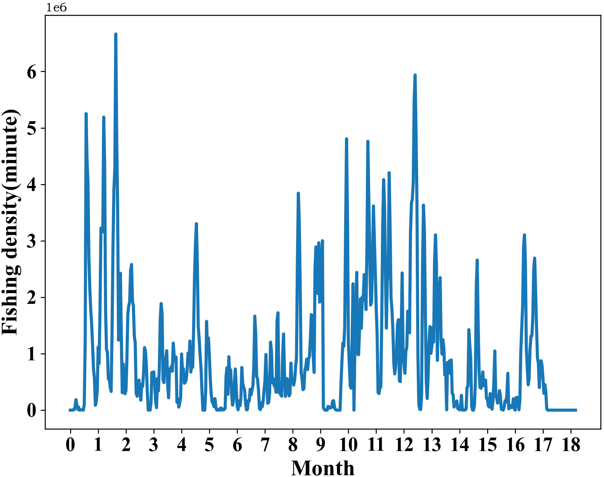
Figure 4 Daily fishing effort variation in a hotspot region.

2.3 Evaluation methods

The proposed model is trained using the VMS dataset in the East China Sea, which covers the period from September 1, 2015, to May 30, 2016, alongside associated hydrological factor datasets obtained from the Copernicus Climate Data Store. This training dataset is utilized for two primary purposes: firstly, to evaluate the impact lag in the influence of marine hydrological factors on fishing effort distributions, and secondly, to train the prediction model. The loss function used for training is defined in Equation 14, where Θ represents all learnable parameters. ${\widehat{X}}_{\tau +l}$ is a prediction for fishing effort distribution on day τ + l, and $X_{\tau +l}$ is the ground truth. We conducted our training using PyTorch version 1.7.0 on an NVIDIA RTX 3090Ti GPU. For optimization during the training process, we employed the Adam optimizer. The initial learning rate was set at 1e-3, and the mini-batch size was chosen as 8.

$\begin{array}{ll}ℒ(\text{Θ})=\frac{1}{L}{\displaystyle \sum _{l=1}^L}\sqrt{\frac{{\sum }_{(i,j)=(1,1)}^{(I,J)}{({\widehat{X}}_{\tau +l}^{(i,j)}-X_{\tau +l}^{(i,j)})}^2}{I\times J}}& (14)\end{array}$

To assess the prediction accuracy, we use the test dataset of the VMS dataset spans September 1, 2016 to May 31, 2017 with the corresponding hydrological factor datasets. We employ Root Mean Squared Error (RMSE) and prediction Error Ratio (ER) across various time periods for evaluation. For any given day τ within the prediction period, RMSEτ and ERτ represent the RMSE and ER for that specific day, as calculated in Equations 15 and 16, respectively. In these equations, $\widehat{X}{\tau }^{(i,j)}$ denotes the predicted fishing effort, and $X{\tau }^{(i,j)}$ indicates the actual fishing effort in grid cell (i,j) for day τ.

For a predicted week beginning on date τ, $\overline{R\text{MS}{\text{E}}_{\tau }}$ and $\overline{\text{E}{\text{R}}_{\tau }}$ are defined as the average RMSE and ER over the seven days of that week, computed as Equations 17 and 18, respectively. Here, L represents the prediction length, i.e., L = 7 days.

Lastly, $\overline{\text{RMS}{\text{E}}_{\tau }}$ and $\overline{\text{ER}}$ are calculated as the average RMSE and ER over all weeks within the test period, as shown in Equations 19 and 20, respectively. In this context, n is the number of weeks in the test period.

$\begin{array}{ll}RMS{E}_{\tau }=\sqrt{\frac{{\sum }_{(i,j)=(1,1)}^{(I,J)}{({\widehat{X}}_{\tau }^{(i,j)}-X_{\tau }^{(i,j)})}^2}{I\times J}}& (15)\end{array}$

$\begin{array}{ll}E{R}_{\tau }=\frac{RMS{E}_{\tau }}{\frac{1}{IJ}{\sum }_{(i,j)=(1,1)}^{(I,J)}{X}_{\tau }^{(i,j)}}& (16)\end{array}$

$\begin{array}{ll}\overline{RMS{E}_{\tau }}=\frac{1}{L}{\displaystyle \sum _{l=1}^L}RMS{E}_{\tau +l}& (17)\end{array}$

$\begin{array}{ll}\overline{E{R}_{\tau }}=\frac{1}{L}{\displaystyle \sum _{l=1}^L}E{R}_{\tau +l}& (18)\end{array}$

$\begin{array}{ll}\overline{RMSE}=\frac{1}{n}{\displaystyle \sum _{i=1}^n}\overline{RMS{E}_{7i+1}}& (19)\end{array}$

$\begin{array}{ll}\overline{ER}=\frac{1}{n}{\displaystyle \sum _{i=1}^n}\overline{E{R}_{7i+1}}& (20)\end{array}$

To demonstrate HyFish’s superior performance, we conducted a comparative analysis with several predictive methods. These studies are categorized into four types: statistical time series prediction, recurrent network prediction, temporal graph-convolution prediction, and spatiotemporal prediction. Given the scarcity of existing methods specifically tailored for fishing effort prediction, we also included urban traffic prediction models in our comparison. All comparative methods undergo training and testing using the identical dataset and platform as HyFish. Given that existing methods only allow for week-level prediction of fishing effort distributions, our comparison mainly focuses on the accuracy metrics for week-level predictions, e.g., $\overline{\text{RMS}{\text{E}}_{\tau }}$ and $\overline{\text{E}{\text{R}}_{\tau }}$. Besides, the results are obtained by meticulously optimizing the parameters for each of the comparative methods. The methods included in the comparison are detailed as follows.

2.3.1 Statistical Time Series Prediction

ARIMA (Kumar and Vanajakshi, 2015) is a well-known model for forecasting time series which combines moving average and auto-regressive components for modeling time series. ARIMA (Kumar and Vanajakshi, 2015) is a well-known model for time series forecasting that integrates moving average and auto-regressive components. It takes the traffic data recorded by sensors as input and predicts future data from these sensors. For comparison, we conceptualize each grid as a sensor and utilize ARIMA to predict future fishing efforts for each individual grid.

2.3.2 Recurrent Network Prediction

LSTM (Shi et al., 2015) represents a standard form of a recurrent neural network, designed to forecast future values based on historical time series data. In our comparative analysis, we adapt the LSTM model to predict future fishing effort distributions. This is achieved by feeding the historical sequence of fishing effort distributions into each timestep of the LSTM. Consequently, the output from the LSTM network provides the predicted future fishing effort distribution.

2.3.3 Temporal Graph-convolution Prediction

T-GCN (Zhao et al., 2019) merges the capabilities of a graph convolutional network with a gated recurrent unit. This combination is designed to effectively capture both the complex topological structures and the dynamic temporal changes in traffic data. In its standard application, T-GCN conceptualizes a road network as a grid graph, with each road segment representing a grid. The traffic flow on each segment is treated as the characteristic feature of that grid. In our experiment, we analogize each grid in the fishing effort distribution to a road in a road network. Here, the fishing effort value in each grid is analogous to the traffic flow on a road, thereby constructing an input and output format that is compatible with the T-GCN model.

2.3.4 Temporal Spatiotemporal Prediction

DMVST-Ne (Yao et al., 2018) presents a taxi demand prediction model that employs a multi-view spatial-temporal prediction framework. This framework is adept at modeling both spatial and temporal relationships and incorporates a semantic view to capture correlations among regions that exhibit similar temporal patterns. In the context of our scenario, the transition of fishing efforts across various grids can be analogized to the total taxi demand across different areas. This parallel allows us to apply the principles of DMVST-Net to the prediction of fishing effort distributions, adapting its methodology to suit the dynamics of fishing activities.

ST-SSL (Ji et al., 2023) concentrates on improving the representation of traffic patterns to accurately reflect spatial and temporal heterogeneity. It introduces a spatial-temporal self-supervised learning framework specifically for traffic prediction. In its typical application, ST-SSL segments an urban area into grids, calculates the traffic flow in each grid region, and then predicts future urban traffic over a specified period. For evaluation, we adapt this methodology to our scenario by treating the fishing effort in different grids as analogous to traffic flow in urban areas. This adaptation allows us to apply ST-SSL to forecast fishing effort distributions.

Earlybird (Zhao et al., 2021) proposes a specialized system aimed at predicting fishing effort distributions on a week-level basis. Grounded in an understanding of the chronological fishing relationships among trawlers, Earlybird employs a Convolutional Neural Network (CNN) as its predictive model. This model is distinctively designed to use the current week’s fishing behaviors of ‘early birds’ as input, forecasting the upcoming week’s fishing effort distributions of all trawlers. This approach underscores the importance of identifying specific behavioral patterns among trawlers to accurately predict short-term fishing efforts.

To analyze the distinct contributions of each component in the HyFish model, we conduct an ablation study. This study systematically evaluates performance across various permutations of network components and critical configurations. We test fundamental elements like the Enc_fish feature extraction module, which processes historical fishing effort distributions, and the Enchyd module, which analyzes sequences from hydrological factor fields such as Sea Surface Height (SSH), Sea Surface Temperature (SST), Sea Surface Salinity (SSS), and current fields. Key configurations assessed included the criteria for selecting input sequences of hydrological factor fields—whether they correspond with their impact delays or match the historical fishing effort distribution period—and the activation of the attention network in the fusion component.

The test networks fell into five primary categories: (1) A network using only Enc_fish, focusing on historical fishing effort distribution sequences and excluding hydrological factors. (2) Networks incorporating Enc_hyd for a single hydrological factor sequence, considering its specific impact lag. This resulted in four unique networks, one for each factor. (3) Networks combining Enc_fish with Enc_hyd handling two types of hydrological factors, forming six different configurations. (4) Networks integrating both Enc_fish with Enc_hyd with all possible inputs, differing in hydrological field sequence selection—one matched the historical fishing effort period, while the other is selected based on impact lag. (5) The full HyFish model, which activates the attention module in the fusion block, differing from the above categories.

In total, we constructed 14 distinct networks based on these combinations and key settings, allowing for a comprehensive evaluation of each component’s individual and collective contributions within the HyFish model. Each network is trained and tested using the same dataset as HyFish.

3 Results and discussion

In this section, we begin by discussing the results of the impact lag calculation, which determines the time lag between marine hydrological features and the fishing effort distribution. Next, we present the predictions of the fishing effort distribution and evaluate the model’s performance through comparison with previous methods and ablation experiments. Finally, we assess the design parameters of HyFish.

3.1 Impact lag for each hydrological factor

We perform a correlation analysis on the entire train set to determine the impact lag for each hydrological factor. The correlation ratios ρ over different impact delays are shown in Figure 5.

Figure 5

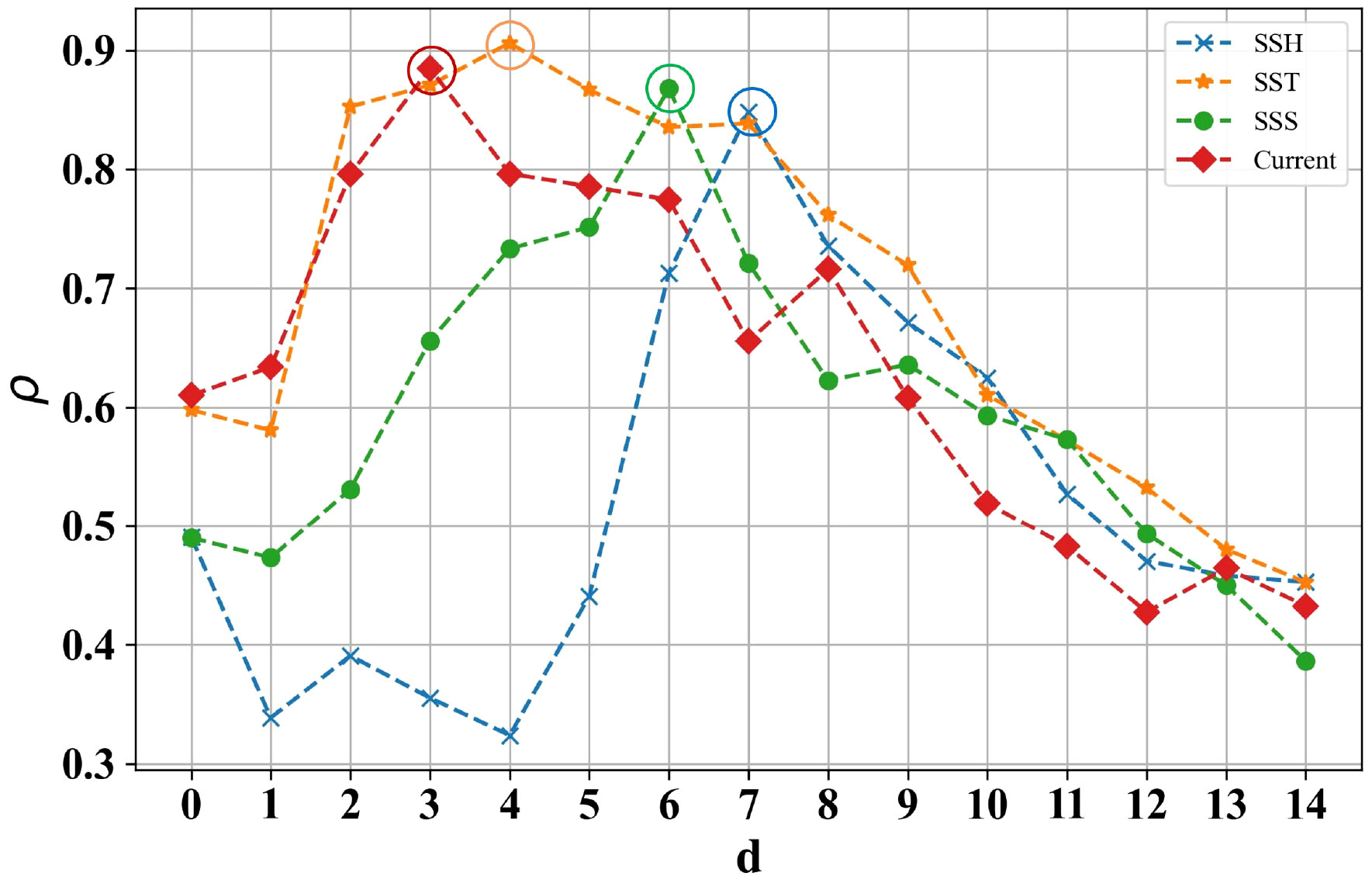
Figure 5 Correlation ratios over different impact delays. Larger ρ, higher impact of hydrological factor filed sequences on fishing effort distributions at that impact delay. The impact delay corresponding to the maximum ρ labels the optimal impact lag d^*.

The correlation analysis reveals that the correlation ratio (ρ) for SST and Current remains consistently above or around 0.8 within the impact lags of 3-6 days. This finding confirms that the variations in SST and Current fields have a significant and relatively short-term impact on the distribution of fishing effort. The observed influence can be attributed to the fact that variations in SST and Current fields directly affect the flow patterns and energy exchange in the marine environment, thereby modifying fishing activities. The optimal impact lag of Current and SST are 3 and 4 days with corresponding correlation ratios of 89% and 91%, i.e. $d_C^{\ast }=3$ and $d_T^{\ast }=4$.

When examining SSS and SSH, their correlations become more pronounced with larger impact lags, typically within the range of 5-7, 6-8 days, respectively. Compared to SST and Current, SSH and SSS exhibit a slightly weaker influence with a longer time lag. This comes from the relatively small variations in SSH and SSS in the short term. Subtle changes in these factors may not have a significant immediate impact on fish aggregation. However, over time, the cumulative changes in SSH and SSS are more likely to affect fish aggregation and distribution patterns. Consequently, the optimal impact lags for SSS and SSH are determined to be 6 and 7 days, respectively, with corresponding correlation ratios of 86% and 85%, respectively. Thus, $d_S^{\ast }=6$ and $d_H^{\ast }=7$ are identified as the optimal impact lags. Hence, the optimal impact lags $d_H^{*}=7,d_T^{*}=4,d_S^{*}=6$, and $d_C^{*}=3$ will be employed to determine the input sequences of the corresponding marine hydrological field sequences in the predictive model.

3.2 Results of fishing effort distribution prediction

To evaluate the performance of daily prediction, we first present the ER_τ distribution for each day of all the predicted weeks. Then we provide the weekly average prediction results and illustrate specific examples.

Figure 6 displays the ER_τ distribution for each day of the predicted week, showing that the ER_τ is lowest on the first day and gradually increases as the time progress, reaching its maximum on the 7th day. This is because the model uses the historical fishing effort distribution from the previous 14 days to predict the first day, and then uses the prediction result of the first day as input to predict the next day, and so on until the 7th day. This iterative prediction process leads to error accumulation, resulting in the increasing ER_τ.

Figure 6

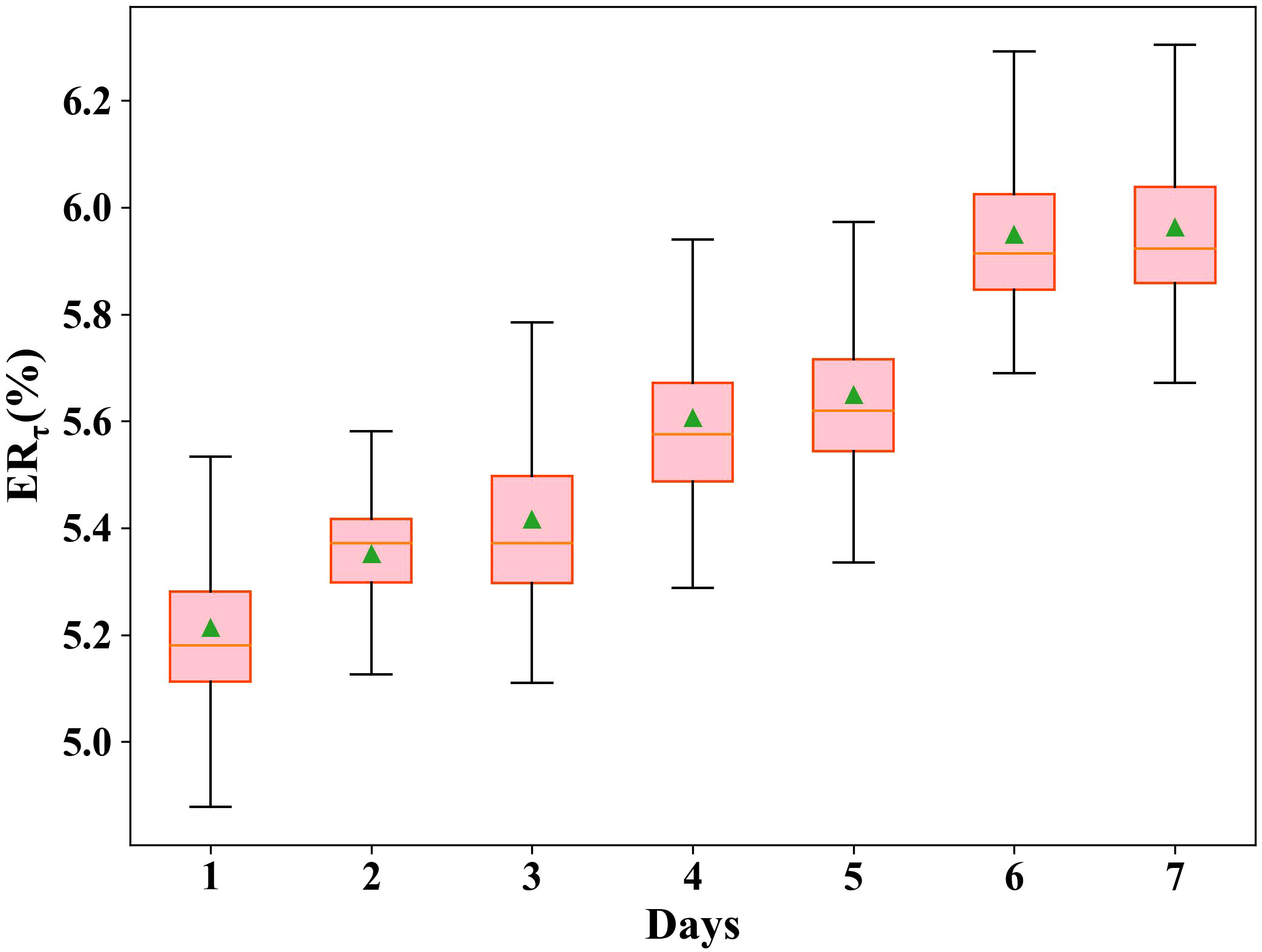
Figure 6 Prediction error ratio distribution for each day in the predicted week across all test period. ER_τ: prediction error ratio on day τ in a predicted week.

Figure 7A shows the $\overline{\text{RMS}{\text{E}}_{\tau }}$ and $\overline{\text{E}{\text{R}}_{\tau }}$ across each week in the test dataset. The $\overline{\text{RMS}{\text{E}}_{\tau }}$ are all below 19, while the $\overline{\text{E}{\text{R}}_{\tau }}$ are all below 10%. The average $\overline{\text{E}{\text{R}}_{\tau }}$ is 5.96%, which proves that HyFish can predict the distribution of future fishing effort accurately. Specifically, we find that the largest and smallest $\overline{\text{RMS}{\text{E}}_{\tau }}$ happen in the 8th and 21st week, respectively. We visualize the actual and difference (difference=|actualprediction|) fishing effort distributions for each day in these two weeks in Figure 8. For the 8th week, from Figures 8A, B, it can be observed that the predicted fishing effort distribution is not significantly different from the actual distribution, with a relatively small numerical gap. which confirm that HyFish captures the trend of fishing effort distribution. We further depict the average fishing effort over grids in Figure 7B. It shows the largest average fishing effort happens in the 8th week. This explains the largest $\overline{\text{RMS}{\text{E}}_{\tau }}$ in the 8th week because the deep learning model exhibits deficiency to capture the future maximum. The $\overline{\text{E}{\text{R}}_{\tau }}$ of 8th week is relatively low of 5.91%.

Figure 7

Figure 7 Prediction results for each week in the test period with ground truth. (A) Average prediction RMSE and ER per grid per day for every week in the test period. (B) Ground truth of average fishing effort per grid per day for every week in the test period.

Figure 8

Figure 8 Comparison between ground truth and the difference of predicted fishing effort distributions for two specific weeks. (A) Ground truth of fishing effort distribution of the 8th week. (B) Difference (| actural prediction|) of fishing effort distributions for the 8th week. (C) Ground truth of fishing effort distribution of the 21st week. (D) Difference (|actual - prediction|) of fishing effort distributions of the 21st week. The unit of measurement for the hotness map is in minutes.

In contrast, for the 21st week, Figures 8C, D display a more noticeable difference between the predicted and actual fishing effort distributions. This is primarily characterized by the predicted fishing effort covering a broader fishing ground, and there are notable numerical disparities as well. Most fishing activities only appear in the nearshore regions in Figure 8C. The reason is that this week includes the Chinese Spring Festival, which is the most important public holiday for the Chinese. Many fishing activities stop during the Chinese Spring Festival. Previous research (Kroodsma et al., 2018) also pointed out the lack of fishing activities during the Chinese Spring Festival. Therefore, the 21st week has the highest $\overline{E{R}_{\tau }}$ (9.92%).

3.3 Results of comparison

Table 1 shows the results of HyFish compared to previous research. Specifically, ARIMA and LSTM perform poorly (i.e., have a $\overline{\text{RMSE}}$ of 131.786 and 113.465, respectively), as they only consider temporal dependence. T-GCN and DMVST-Net further consider spatial features via graph convolution and semantic view, therefore achieving better performance. However, they only concern with the single input of traffic distribution. ST-SSL achieves better performance because it comprehensively considers spatial and temporal heterogeneity. Earlybird achieves the best performance because it takes into account the fishing characteristics of the vessels. It introduces the concept of “fishing chronology among trawlers” and tracks early birds to make targeted predictions for the fishing effort distribution. However, these methods have not taken into account the impact of hydrological factors. In contrast, HyFish not only effectively incorporates hydrological factors into the fishing effort distribution prediction through correlation analysis, but also utilizes a sophisticated network architecture. As a result, HyFish outperforms these methods, achieving a lower $\overline{\text{RMSE}}$ of 16.936 and a lower $\overline{\text{ER}}$ of 6.0%.

Table 1

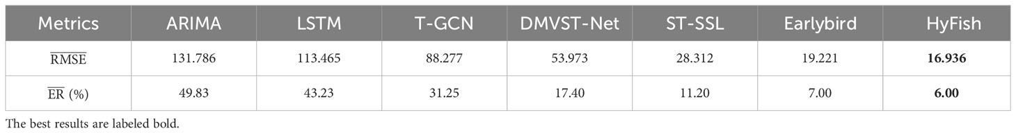
Table 1 The average RMSE, ER compared with different methods.

Figure 9 further compares the week-by-week prediction on $\overline{\text{RMS}{\text{E}}_{\tau }}$ of all the comparing methods for visual clarity. They all have the lowest $\overline{\text{RMS}{\text{E}}_{\tau }}$ in the 21st or 22nd week due to the low average fishing effort distribution during the period of the Chinese Spring Festival. ARIMA and LSTM exhibit high variances on $\overline{\text{RMS}{\text{E}}_{\tau }}$ across all weeks. T-GCN, DMVST-Net, ST-SSL and Earlybird have lower $\overline{\text{RMS}{\text{E}}_{\tau }}$ and variance, compared to the ARIMA and LSTM. The $\overline{\text{RMS}{\text{E}}_{\tau }}$ of HyFish are almost the lowest for all the weeks. Moreover, it shows that the proposed method achieves more stability in prediction compared to all the other models.

Figure 9

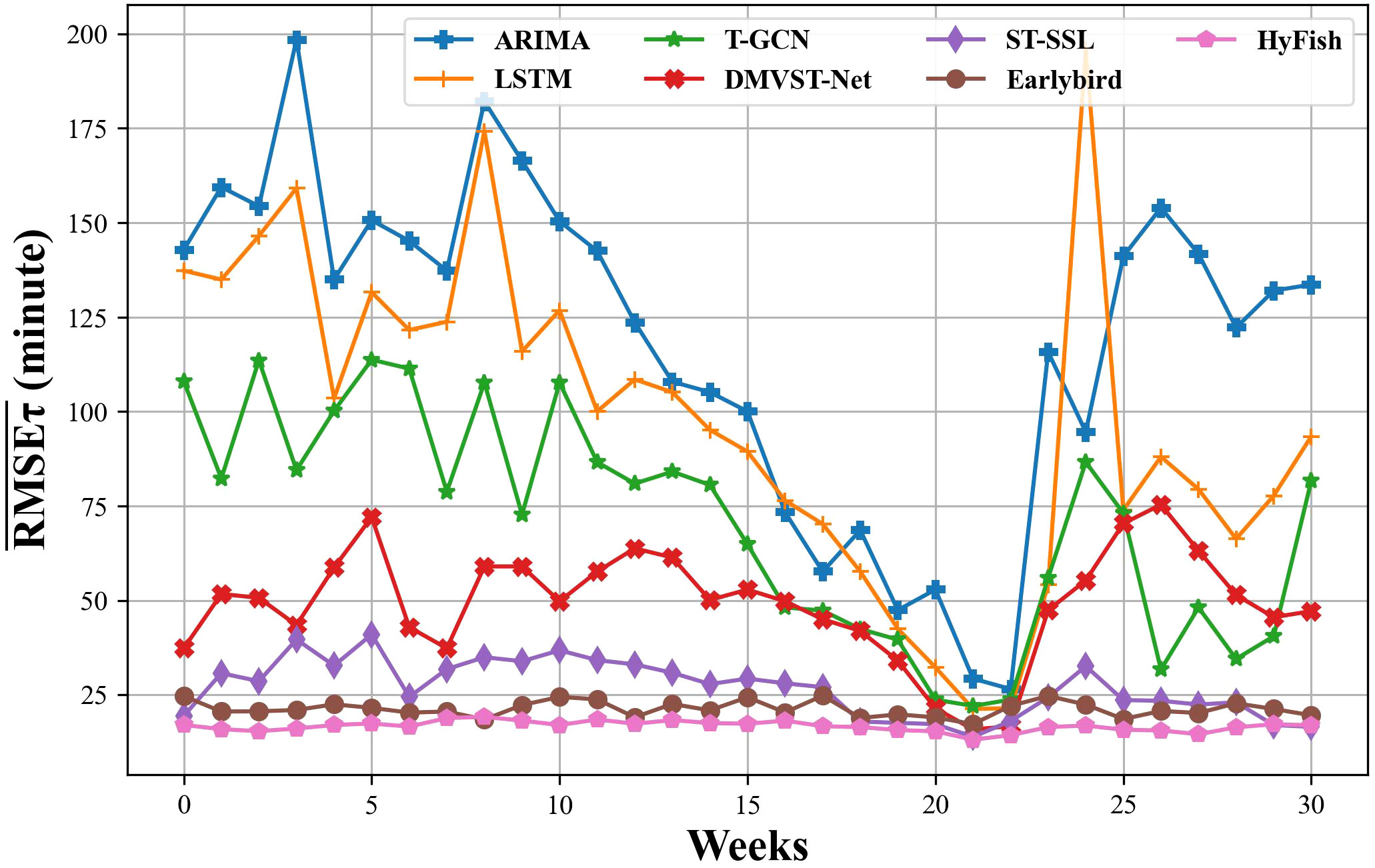
Figure 9 Average prediction RMSE compared with previous methods for every week in the test period. All methods performed best in the 21st or 22nd week. $\overline{RMS{E}_{\tau }}$: Average prediction RMSE for a specific week τ.

3.4 Results of ablation study

The results for each network proposed in the ablation study are systematically compared in Table 2. In this table, every row represents the outcomes of a specific combination of network components within HyFish. Row 1 is the least desirable, with an $\overline{\text{RMSE}}$ of 18.311 and an $\overline{\text{ER}}$ of 6.50%. But it still leads to more accurate predictions than previous methods in Table 1. This improvement can be attributed to the adoption of multiple residual blocks within Enc_fish, which effectively addresses both the proximity and remote challenges in fishing behavior.

Table 2

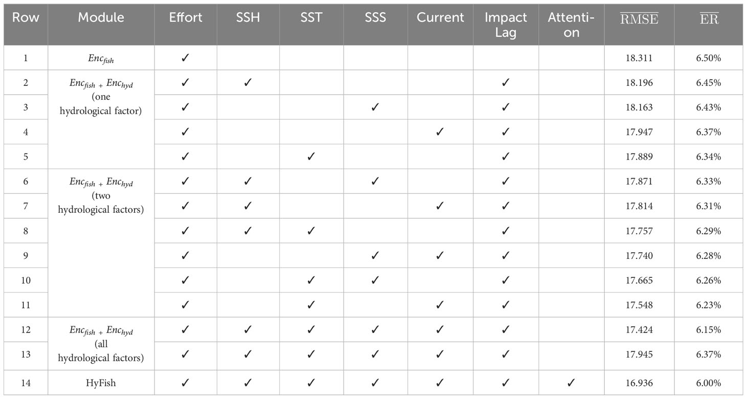
Table 2 Ablation studies.

By observing the results, it’s evident that Rows 2-5 in Table 2 yield better accuracy than using only the fishing effort distribution as input (Row 1), and the combination of Enc_fish + Enc_hyd, utilizing historical fishing effort distributions and the SST field (Row 5), yields the most favorable results, achieving an ($\overline{\text{RMSE}}$) of 17.889 and an ($\overline{\text{ER}}$) of 6.34%. This indicates the contributions of all hydrological factor fields to the prediction and highlights that the improvement from SST is the most significant. This observation not only aligns with the conclusion from Section 3.1, but also corresponds to the significant and immediate influence of SST on fishing effort distribution (Iiyama et al., 2018).

Notably, the predictions of Rows 6-11 surpass those obtained by using only one hydrological factor. Besides, Enc_fish + Enc_hyd with historical fishing effort distributions, SST, and Current fields (Row 11) performs the best with an $\overline{\text{RMSE}}$ of 17.548 and an $\overline{\text{ER}}$ of 6.23%. This illustrates the effectiveness of combining any pair of hydrological factors and underscores that the combination of SST and Current provides the most notable improvement. This observation is consistent with the findings in Section 3.1, where it was concluded that both SST and Current exhibit shorter impact lags and stronger influence on fishing effort distribution.

As presented in Table 2, the performance of integrating features from all hydrological factor fields (Row 12) surpasses that of using only two hydrological factors. This indicates the utility of combining all factor fields for predicting fishing effort distribution, as well as validating the efficacy of the Enc_hyd module. Furthermore, when comparing Row 12 and Row 13, it is evident that the performance of Row 12 ($\overline{\text{RMSE}}$ of 17.424), which incorporates impact lag, is significantly better than Row 13 ($\overline{\text{RMSE}}$ of 17.945). Additionally, it can be observed that the performance of Row 13, which does not incorporate impact lag, suddenly drops to a level similar to using only Current (Row 4). Referring to Figure 5, the impact lag for SSH and SSS is 6 to 7 days. Therefore, without using impact lag, the input historical sequences only contain half of the sequences that have impact on fishing effort distribution as demonstrated by correlation analysis. This leads to a significant decrease in the contribution of these two factors to predictions and results in a reduction in prediction accuracy. It validates the usefulness of impact lag.

Encompassing all modules of HyFish, Row 14 demonstrates the lowest error for $\overline{\text{RMSE}}$. We also plotted the weights of the four hydrological factors captured by the attention mechanism at different time steps of LSTM in Encoder as shown in Figure 10. It is evident that the attention mechanism consistently computes the weights at different time steps effectively, and each hydrological factor has an impact on fishing effort distribution, with SST and Current exhibiting the highest influence weights, followed by SSH and SSS. This observation aligns with the findings in Section 3.1 and confirms the effectiveness of integrating the attention mechanism.

Figure 10

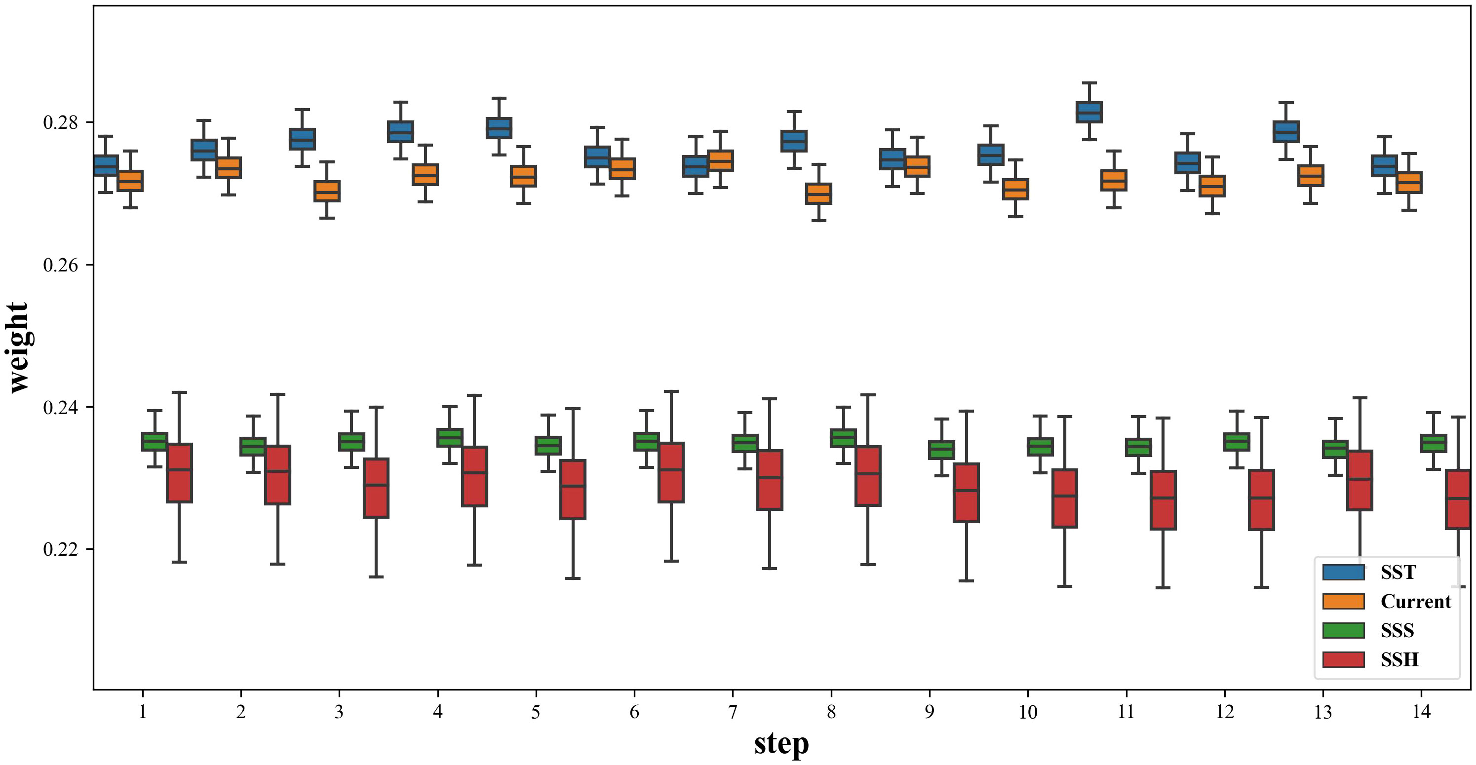
Figure 10 Weight distribution of attention on four hydrological factors at different time steps of LSTM in Encoder. The larger the weight, the greater the impact of the change in the hydrological factor on the fishing effort distribution.

3.5 Results of parameters evaluation

In this section, we study how the input sequence length for Encoder, the output sequence length for Decoder and the layers for feature extraction network affect the performance of HyFish.

Figure 11A shows the $\overline{\text{RMSE}}$. with respect to the input sequence length (P) for Encoder. We can see that when the length is 14 days, our method achieves the best performance. This is because the sequence of 14 days includes the majority of complete voyage of trawlers, allowing the model to learn adequate temporal dependencies, which tends to result in a decrease in $\overline{\text{RMSE}}$. However, as the sequence length reaches around 20 days, there is a decline in performance. One potential reason is that when considering longer time dependencies, the model may overfit.

Figure 11

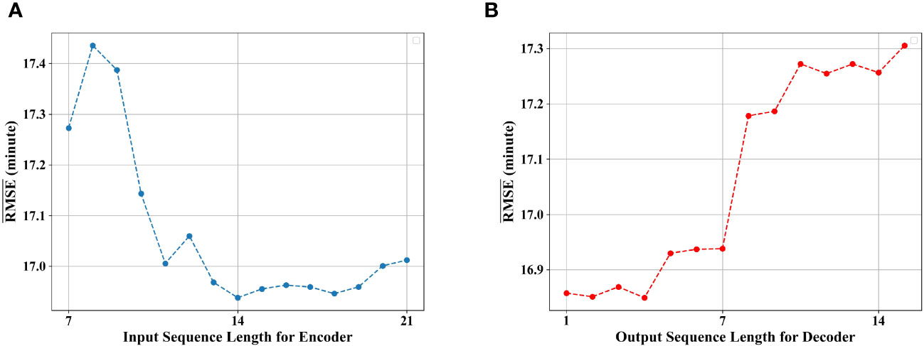
Figure 11 Prediction $\overline{\text{RMSE}}$ corresponding to different lengths of model input and output. $\overline{\text{RMSE}}$: average prediction RMSE over all weeks in the test period. (A) $\overline{\text{RMSE}}$ with respect to input sequence length for Encoder. (B) $\overline{\text{RMSE}}$ with respect to output sequence length for Decoder.

Figure 11B illustrates the impact of the output sequence length (L) on prediction. We can observe that the $\overline{\text{RMSE}}$ fluctuates slightly when the output sequence length is 1-4 days. As the output length exceeds four days, the $\overline{\text{RMSE}}$ slightly increases but remains at a relatively low level. However, when the output sequence length surpasses seven days, the error significantly increases and continues to rise thereafter. Since the decoder operates in an iterative prediction manner, longer output sequences lead to more accumulated errors. We set L to 7, providing sufficient forward-looking information for fishery management authorities to make dynamic adjustments.

Our intuition is that the deeper the network, the more spatial features it can capture. However, increasing the network depth also means more parameters to learn, which may lead to overfitting. In section 2.2.4, we empirically set the number of residual blocks as 3 (b=3), inspired by Figure 3, which is enough to cover most of the daily voyages of fishing vessels. To validate the reasonableness of this number, we plotted the $\overline{\text{RMSE}}$ with different combinations of the numbers of residual blocks. From Table 3, we can observe that initially, as the number gradually increases, the prediction error decreases. The best $\overline{\text{RMSE}}$ is achieved when the numbers of residual blocks for Enc_fish and Enc_hyd are both set to 3. However, further increasing the depths leads to a decline in performance due to overfitting of the prediction model.

Table 3

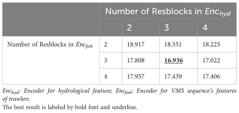
Table 3 $\overline{\text{RMSE}}$ with respect to different number of Resbloks in Enc_fish and Enc_hyd.

3.6 Potential applications

Due to its high prediction accuracy, HyFish not only excels in tracking the evolving patterns of fishing effort but also offers a range of potential applications when integrated with various types of data. For instance (Cimino et al., 2019), utilized historical fishing effort data to monitor activities within protected areas. Similarly, Russo et al. (2019) employed historical fishing effort data to study its impact on key benthic species, thereby uncovering crucial trends in yield, productivity, and the overexploitation rates of demersal stocks. When integrated with data on protected regions or benthic species, HyFish can assist fisheries management in preemptively directing fishing activities in critical areas on a detailed timescale. This can aid in ensuring the sustainable development of biological resources through dynamic adjustments in fishing quotas and other policy measures. Moreover, as shown in studies by (De la Puente et al., 2020) and (Ellis and Wang, 2006), the analysis of historical fishing effort and catch volume is crucial for assessing the economic impact of fishing activities in a specific region. Beyond analyzing historical data, HyFish can also offer forecasts of future target catches for economic evaluations, especially when integrated with data on fishery resource distributions.

Although our system concentrates on the otter trawlers in the East China Sea, the system has the potential to migrate to other regions. The migration only requires determining the parameters of spatial resolution, voyage period, and the number of grids crossed by fishing vessels in a day. By employing local hydrological factors and conducting correlation analysis, the impact lag can be calculated, followed by retraining the model to predict the fishing effort distribution for the new area.

Furthermore, the presence and abundance of biological resources like plankton and microorganisms are key factors to determine the location and timing of fishing activities. Changes in species distribution, driven by migration, breeding cycles, or environmental shifts, significantly influence fishing efforts. It is important to quantify how the distribution of biological resources impacts fishing effort distribution. However, data from marine biological resource surveys are often constrained by the methods used and typically cover a narrower spatial and temporal range compared to hydrological factor data. Additionally, the distribution of biological resources is to some extent influenced by hydrological factor fields. Consequently, our current focus is on the impact of hydrological factor fields in predicting fishing effort distribution. In future work, we aim to delve deeper into the quantitative impact of biological resources on fishing effort distribution and incorporate this understanding into our prediction model through advanced deep-learning components.

4 Conclusion

This study introduces HyFish, a predictive system designed for daily forecasting of fishing effort distributions in the upcoming week. We start with an extensive spatiotemporal analysis to quantify the relationship between hydrological factors and fishing efforts, establishing a foundation for our deep-learning model. The model employs residual networks and Long Short-Term Memory (LSTM) networks, adeptly handling the spatial and temporal dynamics of fishing activities and the influence of hydrological factors. When applied to a comprehensive dataset from the East China Sea, HyFish demonstrated remarkable precision, achieving a daily prediction error ratio of just 5.6% consistently throughout the evaluation period. Looking ahead, our future research will focus on integrating biological resource distribution into the model, aiming to further enhance its predictive capability.

Data availability statement

The original contributions presented in the study are included in the article/supplementary materials, further inquiries can be directed to the corresponding author/s.

Author contributions

YS: Methodology, Writing – review & editing, Software, Writing – original draft. FH: Methodology, Writing – review & editing. ZZ: Data curation, Writing – review & editing. YJ: Writing – review & editing. SZ: Resources, Writing – review & editing. HH: Resources, Writing – review & editing.

Funding

The author(s) declare financial support was received for the research, authorship, and/or publication of this article. This work has been supported by National Natural Science Foundation of China (Grant No. 41976185) and the graduate education quality improvement program of Sanya Oceanographic Institution, Ocean University of China (Grant No. SOIYK009).

Acknowledgments

I would like to appreciate the dedicated efforts of my advisor in revising this paper, as well as the assistance provided by my colleagues in the same academic field.

Conflict of interest

Author SZ is employed by the company Qingdao Network Communication Technology Co. Ltd.

The remaining authors declare that the research was conducted in the absence of any commercial or financial relationships that could be construed as a potential conflict of interest.

Publisher’s note

All claims expressed in this article are solely those of the authors and do not necessarily represent those of their affiliated organizations, or those of the publisher, the editors and the reviewers. Any product that may be evaluated in this article, or claim that may be made by its manufacturer, is not guaranteed or endorsed by the publisher.

References

Bongaarts J. (2019). Ipbes 2019. summary for policymakers of the global assessment report on biodiversity and ecosystem services of the intergovernmental science-policy platform on biodiversity and ecosystem services. Population Dev. Rev. 45, 680–681. doi: 10.1111/padr.12283

CrossRef Full Text | Google Scholar

Britz D., Goldie A., Luong M.-T., Le Q. (2017). “Massive exploration of neural machine translation architectures.” in Proceedings of the 2017 conference on empirical methods in natural language processing. Palmer M., Hwa R., Riedel S.. eds. (Copenhagen, Denmark: Association for Computational Linguistics), 1442–1451. doi: 10.18653/v1/D17-1151

CrossRef Full Text | Google Scholar

Chen Y., Xinjun C., Lixin G., Ran W., Weiping X., Liangqi X. (2017). Preliminary analysis of predict model of fishing effort spatial distribution for skipjack tuna catches by purse seine in the west-central pacific ocean. Haiyang Xuebao 39, 32–45. doi: 10.3969/j.issn.0253-4193.2017.10.003

CrossRef Full Text | Google Scholar

Cimino M. A., Anderson M., Schramek T., Merrifield S., Terrill E. J. (2019). Towards a fishing pressure prediction system for a western pacific eez. Sci. Rep. 9, 461. doi: 10.1038/s41598-018-36915-x

PubMed Abstract | CrossRef Full Text | Google Scholar

De la Puente S., López de la Lama R., Benavente S., Sueiro J. C., Pauly D. (2020). Growing into poverty: Reconstructing Peruvian small-scale fishing effort between 1950 and 2018. Front. Mar. Sci. 7, 681. doi: 10.3389/fmars.2020.00681

CrossRef Full Text | Google Scholar

Demirel N., Nauen C. E., Palomares M. L. D. (2023). Fishing effort and the evolving nature of its efficiency. Front. Mar. Sci. 10, 1180174. doi: 10.3389/fmars.2023.1180174

CrossRef Full Text | Google Scholar

Dinmore T., Duplisea D., Rackham B., Maxwell D., Jennings S. (2003). Impact of a large-scale area closure on patterns of fishing disturbance and the consequences for benthic communities. ICES J. Mar. Sci. 60, 371–380. doi: 10.1016/S1054-3139(03)00010-9

CrossRef Full Text | Google Scholar

Ellis N., Wang Y.-G. (2006). Effects of fish density distribution and effort distribution on catchability. ICES J. Mar. Sci. 64, 178–191. doi: 10.1093/icesjms/fsl015

CrossRef Full Text | Google Scholar

Gers F. A., Schmidhuber J., Cummins F. (2000). Learning to forget: Continual prediction with lstm. Neural Comput. 12, 2451–2471. doi: 10.1162/089976600300015015

PubMed Abstract | CrossRef Full Text | Google Scholar

Hong F., Wu Z., Tian Y., Huang H., Liu C., Jiang R., et al. (2019). “Spatio-temporal fine-grained fishing vessel density prediction through joint residual network,” in OCEANS 2019-Marseille (Piscataway, NJ: IEEE), 1–5.

Google Scholar

Iiyama M., Zhao K., Hashimoto A., Kasahara H., Minoh M. (2018). “Fishing spot prediction by sea temperature pattern learning,” in 2018 OCEANS - MTS/IEEE Kobe Techno-Oceans (OTO) (Piscataway, NJ: IEEE), Vol. 1–4. doi: 10.1109/OCEANSKOBE.2018.8559299

CrossRef Full Text | Google Scholar

Ji J., Wang J., Huang C., Wu J., Xu B., Wu Z., et al. (2023). “Spatio-temporal self-supervised learning for traffic flow prediction,” in Proceedings of the AAAI Conference on Artificial Intelligence (Menlo Park: AAAI), vol. 37, 4356–4364.

Google Scholar

Jin J., Zhou W., Jiang B. (2021). “An overview: Maritime spatial-temporal trajectory mining,” in Journal of Physics: Conference Series (Bristol: IOP Publishing), 1757, 012125.

Google Scholar

Kaiser M. J., Ramsay K., Richardson C., Spence F., Brand A. (2000). Chronic fishing disturbance has changed shelf sea benthic community structure. J. Anim. Ecol. 69, 494–503. doi: 10.1046/j.1365-2656.2000.00412.x

CrossRef Full Text | Google Scholar

Kroodsma D. A., Mayorga J., Hochberg T., Miller N. A., Boerder K., Ferretti F., et al. (2018). Tracking the global footprint of fisheries. Science 359, 904–908. doi: 10.1126/science.aao5646

PubMed Abstract | CrossRef Full Text | Google Scholar

Kumar S. V., Vanajakshi L. (2015). Short-term traffic flow prediction using seasonal arima model with limited input data. Eur. Transport Res. Rev. 7, 1–9. doi: 10.1007/s12544-015-0170-8

CrossRef Full Text | Google Scholar

Leitão F. (2023). “Environmental conditions affect striped red mullet (mullus surmuletus) artisanal fisheries,” in Oceans (Basel, Switzerland: MDPI), 4, 220–235.

Google Scholar

Li X., Zhou L., Xiao Y., Wu W., Su F., Shi W. (2021). Spatial characteristics mining of fishing intensity in the northern south China sea based on fishing vessels ais data. J. Geoinformation Sci. 23, 850–859. doi: 10.12082/dqxxkx.2021.200328

CrossRef Full Text | Google Scholar

Rijnsdorp A., Buys A., Storbeck F., Visser E. (1998). Micro-scale distribution of beam trawl effort in the southern north sea between 1993 and 1996 in relation to the trawling frequency of the sea bed and the impact on benthic organisms. ICES J. Mar. Sci. 55, 403–419. doi: 10.1006/jmsc.1997.0326

CrossRef Full Text | Google Scholar

Rubenstein S. R. (2021). Energetic impacts of passage delays in migrating adult Atlantic Salmon (Orono: The University of Maine).

Google Scholar

Russo E., Monti M. A., Mangano M. C., Raffaetà A., Sarà G., Silvestri C., et al. (2020). Temporal and spatial patterns of trawl fishing activities in the adriatic sea (central mediterranean sea, gsa17). Ocean Coast. Manage. 192, 105231. doi: 10.1016/j.ocecoaman.2020.105231

CrossRef Full Text | Google Scholar

Russo T., Carpentieri P., D’Andrea L., De Angelis P., Fiorentino F., Franceschini S., et al. (2019). Trends in effort and yield of trawl fisheries: a case study from the mediterranean sea. Front. Mar. Sci. 6, 153. doi: 10.3389/fmars.2019.00153

CrossRef Full Text | Google Scholar

Shi X., Chen Z., Wang H., Yeung D.-Y., Wong W.-K., Woo W.-C. (2015). Convolutional lstm network: A machine learning approach for precipitation nowcasting. Adv. Neural Inf. Process. Syst. 28, 802–810. doi: 10.48550/arXiv.1506.04214

CrossRef Full Text | Google Scholar

Stefansson G., Rosenberg A. A. (2005). Combining control measures for more effective management of fisheries under uncertainty: quotas, effort limitation and protected areas. Philos. Trans. R. Soc. B: Biol. Sci. 360, 133–146. doi: 10.1098/rstb.2004.1579

CrossRef Full Text | Google Scholar

Vianna G. M., Hehre E. J., White R., Hood L., Derrick B., Zeller D. (2020). Long-term fishing catch and effort trends in the republic of the Marshall Islands, with emphasis on the small-scale sectors. Front. Mar. Sci. 6, 828. doi: 10.3389/fmars.2019.00828

CrossRef Full Text | Google Scholar

Yao H., Wu F., Ke J., Tang X., Jia Y., Lu S., et al. (2018). “Deep multi-view spatial-temporal network for taxi demand prediction,” in Proceedings of the AAAI conference on artificial intelligence (Menlo Park: AAAI), Vol. 32.

Google Scholar

Yuan H., Hui L., Shuo Z., Guanqi C. (2021). Fisheries forecasting method based on deep learning and canonical correlation analysis. J. Dalian Ocean Univ. 36, 670–678. doi: 10.16535/j.cnki.dlhyxb.2020-326

CrossRef Full Text | Google Scholar

Zhao Z., Hong F., Huang H., Liu C., Feng Y., Guo Z. (2021). Short-term prediction of fishing effort distributions by discovering fishing chronology among trawlers based on vms dataset. Expert Syst. Appl. 184, 115512. doi: 10.1016/j.eswa.2021.115512

CrossRef Full Text | Google Scholar

Zhao L., Song Y., Zhang C., Liu Y., Wang P., Lin T., et al. (2019). T-gcn: A temporal graph convolutional network for traffic prediction. IEEE Trans. Intelligent Transportation Syst. 21, 3848–3858. doi: 10.1109/TITS.2019.2935152

CrossRef Full Text | Google Scholar