A comparison of adenosine triphosphate with other metrics of microbial biomass in a gradient from the North Atlantic to the Chesapeake Bay

Bochdansky, Alexander B.; Beecher, Amber A.; Calderon, Joshua R.; Stouffer, Alison N.; Washington, NyJaee N.

doi:10.3389/fmars.2024.1288812

ORIGINAL RESEARCH article

Front. Mar. Sci., 31 January 2024

Sec. Marine Biogeochemistry

Volume 11 - 2024 | https://doi.org/10.3389/fmars.2024.1288812

A comparison of adenosine triphosphate with other metrics of microbial biomass in a gradient from the North Atlantic to the Chesapeake Bay

Alexander B. Bochdansky^1*

Amber A. Beecher²

Joshua R. Calderon³

Alison N. Stouffer⁴

NyJaee N. Washington⁵

¹Department of Ocean and Earth Sciences, Old Dominion University, Norfolk, VA, United States
²Lake Erie Center, University of Toledo, Oregon, OH, United States
³School of Sustainable Engineering and the Built Environment, Arizona State University, Tempe, AZ, United States
⁴Nicholas School of the Environment, Duke University, Durham, NC, United States
⁵Department of Biological Sciences, Kenneth P. Dietrich School of Arts & Sciences, University of Pittsburgh, Pittsburgh, PA, United States

A new, simplified protocol for determining particulate adenosine triphosphate (ATP) levels allows for the assessment of microbial biomass distribution in aquatic systems at a high temporal and spatial resolution. A comparison of ATP data with related variables, such as particulate carbon, nitrogen, chlorophyll, and turbidity in pelagic samples, yielded significant and strong correlations in a gradient from the tributaries of the Chesapeake Bay (sigma-t = 8) to the open North Atlantic (sigma-t = 29). Correlations varied between ATP and biomass depending on the microscopic method employed. Despite the much greater effort involved, biomass determined by microscopy correlated poorly with other indicator variables including carbon, nitrogen, and chlorophyll. The ATP values presented here fit well within the range of ATP biomass estimates in the literature for similar environments. A compilation of prior research data from a wide range of marine habitats demonstrated that ATP values can be ranked according to broad trophic gradients, from the deep sea to eutrophic inland waters. Using a mass-based conversion factor of 250, the contribution of biomass to overall particulate organic carbon (POC) ranged from 15% to 30% along the gradient, from the open ocean to locations in the Chesapeake Bay respectively. Our data corroborate the notion that ATP, due to its consistency and simplicity, is a promising high-throughput indicator of cytoplasm volume with distinct benefits over cell counts and measures of chlorophyll or POC.

Introduction

Microbial biomass is an important ecological metric, especially in aquatic ecosystems where microbes are the dominant form of living matter (Bar-On and Milo, 2019; Hatton et al., 2021). Yet determining how much living biomass inhabits a specific volume of water is surprisingly difficult. Microscopy is perhaps the most frequently employed technique to estimate biomass, but it typically only encompasses microbial numbers of specific target organisms such as prokaryotes, which can leave others such as eukaryotes unaccounted for.

Prokaryotic and eukaryotic biomass are rarely determined simultaneously, mainly because of the considerable effort and numerous assumptions involved in obtaining biovolumes and converting them into carbon-based biomass (e.g., Andersson and Rudehäll, 1993; Fukuda et al., 1998; González et al., 1998). For prokaryotes, which do not vary greatly in size, the conversion from cell numbers to biomass is relatively straightforward, with values typically constrained to 10 or 20 femtograms (fg) cell^-1 (Christian and Karl, 1994; Fukuda et al., 1998; Herndl et al., 2023). For eukaryotic microbes, however, translating cell numbers into biomass is more problematic as they can display extreme variability in size and shape. In the case of eukaryotes, converting cell counts to cell volumes entails first measuring the dimensions of organisms to calculate biovolume, which requires a series of assumptions, as does converting this data to carbon mass in a second step (e.g., Verity et al., 1992; Menden-Deuer and Lessard, 2000). Overall, the procedure is time-consuming, prone to preservation and staining artifacts, and susceptible to investigator bias.

Where eukaryotic microbes dominate in many coastal surface environments (e.g., Verity et al., 1996b), estimates of microscopic biomass are highly dependent on the accuracy of the determination of cell volumes. Furthermore, in pelagic environments, microscopic techniques are limited to freely suspended microbes. Biomass estimates based on microscopy are much less accurate in samples with high sediment load, in marine snow, flocs, and other organic aggregates, and in benthic systems in which individual microbes may be shaded by organic matrices or sediments. Finally, microscopic determinations of the mass of both prokaryotic and eukaryotic microbes are prone to error if dead cells or “ghosts” are included, as such ghosts may comprise a substantial portion of the overall count (e.g., Zweifel and Hagstrom, 1995).

Other metrics such as chlorophyll and POC also have limitations as biomass indicators. For example, any non-photosynthesizing microbes such as heterotrophs and chemoautotrophs will not be captured by chlorophyll determinations. Chlorophyll levels per cell are highly variable even within the same species, as well as due to photo-acclimation (Falkowski and LaRoche, 1991; Mignot et al., 2014; Cullen, 2015; Estrada et al., 2016). On the other hand POC may include a highly variable, large, and ill-defined pool of organic material, such as detritus, gels, and transparent exopolymer material, that is not considered biomass (Parsons and Strickland, 1962; Odum and de la Cruz, 1963; Nagata and Kirchman, 1997; Volkman and Tanoue, 2002).

One metric that was proposed more than half a century ago as a useful proxy for live biomass is particulate adenosine triphosphate (pATP) (Levin et al., 1964; Holm-Hansen and Booth, 1966; Karl, 2018). It has never been adopted widely in oceanography and has only been used routinely at the Hawaiian Ocean Time Series (Karl et al., 2022). Critics of the ATP method point to variable carbon-to-ATP ratios in live cells; however, the underlying evidence for this variability is sparse (Dawes and Large, 1970; Stuart, 1982; Amy et al., 1983; see Bochdansky et al. (2021) for a critical analysis). In these studies, any difference in per-cell ATP levels was either temporary and small (Dawes and Large, 1970), or large and rather inconsistent compared with other metrics (Amy et al., 1983).

The idea that ATP levels reflect the amount of biomass has recently been strengthened by the realization that ATP is not only the universal currency of cellular energy but also functions as a hydrotrope, keeping macromolecules dissolved in cytoplasm (Patel et al., 2017). This latter function explains why ATP is so abundant in cytoplasm and why it occurs at a much higher concentration than is needed for all cellular metabolism combined (Patel et al., 2017; Pu et al., 2019; Ochs, 2021). Cellular metabolism requires ATP in micromolar concentrations only, yet ATP needs to be maintained at a millimolar concentration in cytoplasm to function as a hydrotrope (Patel et al., 2017). Finally, the concentration of ATP in cytoplasm appears to be surprisingly similar across all living cells, from bacteria to eukaryotic cells, including human erythrocytes (Bochdansky et al., 2021). Cellular ATP therefore represents cytoplasm volume, which in turn is a very reasonable metric of biomass.

To further test the utility of the ATP-biomass method, we measured particulate, dissolved, and total ATP concentrations in surface waters along a gradient from the open ocean to the Chesapeake Bay estuary. Because most ATP surveys are conducted in the open ocean, data for coastal areas and estuaries are rare. We also compare the absolute ATP values against a wide range of environments to determine whether absolute ATP values follow a consistent pattern among ecosystems with different trophic states. Finally, we explore the conversion from ATP to carbon equivalents and discuss the implications of our findings for estimates of living versus non-living organic material.

Methods

Field measurements and bottle collections

Seawater was collected on the research vessel Fay Slover using 5 L Niskin bottles along a gradient from the open ocean near the Chesapeake light tower into the Chesapeake Bay and the James River, in April 2018 and June 2019 (Table 1, Figure 1). Conductivity, temperature, and depth were measured using a SBE 32 CTD equipped with a Wetlabs fluorometer and a Wetlabs transmissometer (650 nm).

Table 1

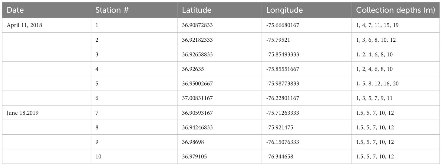
Table 1 Niskin bottle collection depths during the two cruises from the continental shelf to the James River, a tributary of the Chesapeake Bay (Figure 1).

Figure 1

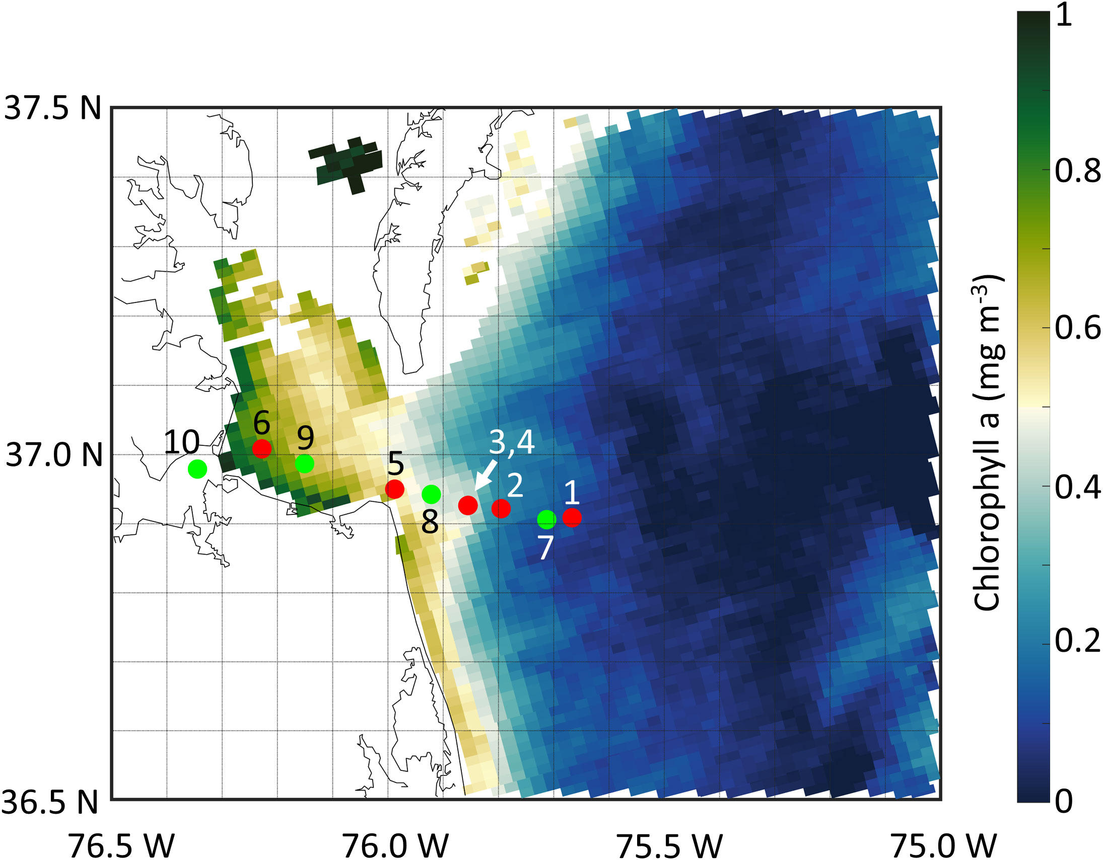
Figure 1 Station map for cruises in April 2018 (red circles) and June 2019 (green circles) superimposed over an ocean color image of chlorophyll a (MODIS) from April 11, 2018. Stations 3 and 4 appear as one symbol as they are only separated by 1 km, straddling the Chesapeake Bay plume front (Figure 2).

Field collection of ATP

ATP samples were processed using the hot-water extraction method described by Bochdansky et al. (2021). Three types of ATP samples were collected: 1) pATP in 5 ml seawater filtered through 0.2 μm pore size polycarbonate filters (Isopore GTTP, 25 mm diam.), 2) dissolved ATP (ATP in the filtrate of 0.2 μm filtration), and 3) 0.5 ml ATP in whole water without filtration. Polycarbonate filters were chosen over GF/F filters because of their higher retention efficiency (Taguchi and Laws, 1988; Lee et al., 1995) and because the volumes filtered were small, to ensure filtration times were kept to a minimum even with the use of the smaller pore size. Five milliliters of each depth were immediately and simultaneously filtered using a filtration manifold (25 mm-diameter filters, stainless steel screen supports) preloaded with the polycarbonate filters. The filters were placed in 15 ml polypropylene centrifuge tubes (Falcon™) within seconds after the water passed. The dissolved ATP was captured in 15 ml polypropylene centrifuge vials placed underneath the filtration manifold and inside the vacuum flasks. The dissolved ATP samples (i.e., the 0.2 μm filtrates) were immersed in a boiling water bath for ~15 minutes immediately after filtration to sterilize the water and inactivate ATPases and then frozen at -80°C until analysis.

In April 2018, approximately 4.5 ml of boiling ultrapure water was quickly added to each centrifuge tube. The tubes were stoppered and transferred to a beaker with boiling water for ~15 minutes for extraction of intracellular ATP and inactivation of ATPases. After extraction, the tubes were cooled to room temperature and then kept frozen at -20°C for transport to the laboratory. Samples were subsequently kept at -80°C until analysis.

In June 2019, instead of boiling on board, filters, filtrates, and whole water samples were collected as above but immediately frozen in liquid nitrogen, transported to the laboratory at -20°C, and stored at -80°C in the lab. Hot-water extraction was then performed on the still frozen samples (i.e., without prior thawing) in the laboratory (see Bochdansky et al., 2021 for details). The shock freezing-boiling treatment breaks up cells more efficiently than boiling alone, which results in higher extraction efficiencies (Bochdansky et al., 2021).

In 2018, 500 μl of water from each bottle was collected and extracted in a boiling hot-water bath before the samples were cooled to room temperature, and then frozen at -20°C. In 2019, 500 μl of water from each bottle was placed in 15 ml centrifuge tubes and shock-frozen in liquid nitrogen. These unfiltered samples thus contained both particulate and dissolved ATP and were labeled total ATP (tATP). All samples were brought to the laboratory in a -20°C freezer and subsequently stored at -80°C in the laboratory. For analysis of the 500 μl shock-frozen samples, boiling hot water was added to the samples and extracted for ~15 minutes in a boiling-water bath.

Particulate and total ATP samples were topped up to 5 ml with ultrapure water using the gradations on the centrifuge tubes and mixed with a vortex mixer. The 500 μl whole-water samples were also diluted to 5 ml with ultrapure water to reduce salt effects that strongly decrease the luminescence yield. It should be noted that the whole-water extraction method used here (for total ATP) requires sufficiently high ATP levels to produce a signal. This was possible because samples were taken in the mesotrophic coastal ocean and in a eutrophic estuary. Such a small amount of water (500 μl) would be insufficient in oligotrophic or deep-sea environments. Hot-water extraction is only one of two methods proposed by Bochdansky et al. (2021). Many of our subsequent collections were based on chemical extraction using phosphorus benzalkonium chloride (P-BAC) instead. Both methods give highly consistent results, with the values from the chemical extraction method exceeding that of the hot water extraction by 20% (Bochdansky et al., 2021). The hot-water method used here has the advantage that measurements of dissolved ATP can be added easily to the protocol as hot water for the inactivation of ATPases is already at hand.

Laboratory analysis of ATP

Fifty microliters of each sample (in triplicates) were transferred to 6 ml pony scintillation vials (Research Products International), and received 3 ml of ultrapure water, and 50 µL of CellTiter-Glo 2.0 (Promega Corporation). Internal standards were used by spiking a fourth vial with 50 µL of samples with 50 µL of 0.0164 µM ATP standard. Using internal standards instead of separate calibration curves corrects for matrix effects that change the luminescence signal caused by the presence of ions, acids, and organic material (Bochdansky et al., 2021). Luminescence was analyzed in a PerkinElmer Liquid Scintillation Analyzer with a single photon counting protocol of 1 minute each. The counter was programmed to cycle samples five times in sequence. We determined that values from the second cycle were the most consistent and were thus subsequently used for all analyses.

ATP was calculated using the formula Equation 1:

\begin{array}{l} A T P (n M) = \frac{[ATP] * (C P M_{s a m p l e} - {\bar{C P M}}_{blank})}{({\bar{C P M}}_{standards} - {\bar{C P M}}_{samples})} * \frac{V_{s t d} * R}{V_{e x t r}}, & (1) \end{array}

where [ATP] is the concentration of the internal standard as determined by spectrophotometry (i.e., 16.4 nM), $C P M_{s a m p l e}$ the photon counts per minute for the sample, ${\bar{C P M}}_{blank}$ the average value of 4 to 6 blanks (50 μl of Celltiter Glo 2.0 reagent added to 3 ml ultrapure water only), ${\bar{C P M}}_{standards}$ the average counts per minute for the standard vials of the same sample type, ${\bar{C P M}}_{samples}$ the average of triplicate values for each sample, V_std the volume of the standard added to the scintillation vial in μl, R the ratio between the volume of the extract (numerator) and the volume of sample filtered (denominator), and V_extr the volume of the extract added to the scintillation vial (in μl; 50 μl of the water extract).

Particulate organic carbon and nitrogen

During the June 2019 cruise, between 75 ml and 250 ml of seawater (less in the inshore and more in the offshore stations) was filtered onto pre-combusted (450°C, 4 hours) GF/F filters. The filters were stored frozen (-20°C) and later dried at 50°C for approximately 2 days. Filters were then rolled in a tin wrap and pressed into pellets to be analyzed in a Europa 20‐20 isotope ratio mass spectrometer (IRMS) equipped with an automated N and C analyzer.

Microscopic organic analysis of biomass

2018 samples

For bacteria abundance, 20 ml of the Niskin bottle sample was added to a 50 ml Falcon tube and preserved with 2% (fin. conc.) formaldehyde. Within 24 hours, 5 ml of the formaldehyde sample (in duplicates) was filtered onto a 25 mm diameter, 0.2 μm pore size, black polycarbonate filter (Isopore type GTBP, Millipore Corp.). The filter was put onto a slide and one drop of Vectashield Antifade Mounting Medium with DAPI (H1200, Vector Laboratories) was applied. A cover slip was added and the slide was stored at -20°C.

The slides were brought to room temperature in a desiccator to remove condensation before immersion oil was added to the cover slips. Bacteria were enumerated under an Olympus BX61 epifluorescence microscope (100 x oil immersion objective, 2 x loupe, 10 x ocular magnification). ToupView (Toup Tek Photonics) imaging software was used to take images of the bacteria slides. Images were analyzed using a custom macro developed for ImageJ software (National Institutes of Health, https://imagej.nih.gov/ij/index.html). This macro inverted the image, converted it into an 8 bit image, applied a FFT Bandpass Filter, binarized the image, and finally applied a watershed feature that outlined each bacterium. The algorithm automatically counted the number of bacteria and the area of each bacterium on each picture. A fixed value of 20 femtogram (fg) carbon per prokaryotic cell was applied (Ducklow, 2000). We preferred the higher value as cell carbon is typically higher in eutrophic systems than in open and deep ocean environments (Ducklow, 2000; Herndl et al., 2023).

For the enumeration of eukaryotes and measurements of size, two types of analysis were performed: epifluorescence and inverted microscopy. The same slides used for the bacteria counts were also used to count eukaryote microbes directly. The eukaryotes were counted if the bright blue spots were at least twice the size (linear dimension) of the bacteria in the image. If a large red fluorescence due to chlorophyll was noticed but there was no noticeable blue nucleus, it was still counted as a eukaryote. Organisms that were completely inside the picture were counted; if an organism landed on the top or left side of the picture and at least ¾ of the organism was visible, then it was counted too. If the organism landed on the right or the bottom of the image and was cut off, then it was not counted. The total number of eukaryotes was taken for each station and depth and a fixed value of 2,200 fg was applied, assuming that the overwhelming majority of these eukaryotes were nanoplankton (Pomeroy, 1974; Fukuda et al., 2007; Sohrin et al., 2010). Given the wide size range in eukaryotes, this step represents a major simplification (see Discussion).

For inverted microscopy, 20 ml sample vials were filled with seawater to the vial shoulder and 6 drops of Lugol’s solution were added to produce a tea-colored solution. Once in the lab, samples were mixed by inversion and 10 ml of the sample was measured into a graduated cylinder. Another 4 drops of Lugol’s solution were added and then topped off with equal-salinity 0.2 μm-filtered artificial seawater. Once the chamber was topped off, a glass plate was placed on the top to make it air-tight and to hold the water column in the settling chamber. After 24–48 hours of settling, the chamber was drained and replaced with a cover slip.

The slide was then processed under an Olympus CK7 inverted microscope equipped with a digital camera (see above). Organisms on the entire slide were imaged and all of those with the following criteria were analyzed. Organisms that were over 9,000 pixels in area (~ 100 μm²) and had a smooth shape to the structure (indicating a cell membrane) were included. For ciliated cells, only the area inside the cell membrane was measured. Diatom cell chains were measured as one composite organism. Each organism on the image was outlined and the area in pixels was recorded. If two or more organisms were identical, then only one would be measured and that measurement would be extrapolated to all identical organisms on the image. Any empty-shelled organisms were excluded. Due to time constraints, only approximately every tenth image was examined, and the results extrapolated to the entire sample. The area in pixels was converted to μm² then the volume was calculated according to Bochdansky et al. (2017a). Volumes were converted into carbon values using Equation 2 (Menden-Deuer and Lessard, 2000):

\begin{array}{l} {Log}_{10} (carbon (pg)) = - 0.665 + 0.939 * {Log}_{10} (volume ({μm}^{3})) & (2) \end{array}

2019 samples

Prokaryote samples were fixed with formaldehyde and slides were prepared and stained with DAPI as described above. Prokaryotes within an area of 0.00025 mm² in thirty random fields were manually counted across the filters for each slide under an Olympus epifluorescence microscope. As with the 2018 samples, bacteria counts were converted to carbon using 20 fg per cell.

For eukaryote biomass estimates, 10 ml of the unfixed sample was filtered through a 0.2 µm GTBP membrane filter as well as a 0.45 µm cellulose nitrate backing filter. When no liquid remained, the pump was switched off and the valves were closed to release the vacuum. One ml of a plasma membrane stain (10.0 µL of CellMask (Invitrogen) in 10 ml of 0.2 μm-filtered 34 ppt artificial seawater) was added to the dry filter and kept for 10 minutes before the valves were opened and the pump was turned on. When the stain was completely filtered, two rounds of 1.0 ml filtered artificial seawater were pipetted evenly over the filters to rinse. Nuclei were counter stained with DAPI and embedded in Vectashield as described above. Slides were kept at -20°C until microscopic examination.

Eukaryote slides were prepared for depths #1, #3, and #5 at each station (actual depths varied), skipping depths in between (Table 1). Thirty randomly selected image pairs, taken with DAPI and TRITC filter sets, were captured per slide using ToupView Imager software (Figure 2). DAPI images were taken to confirm that cell nuclei were present. Cell bodies were delineated using ImageJ (Figure 2) and cell volumes and carbon values calculated as for the Lugol’s samples.

Figure 2

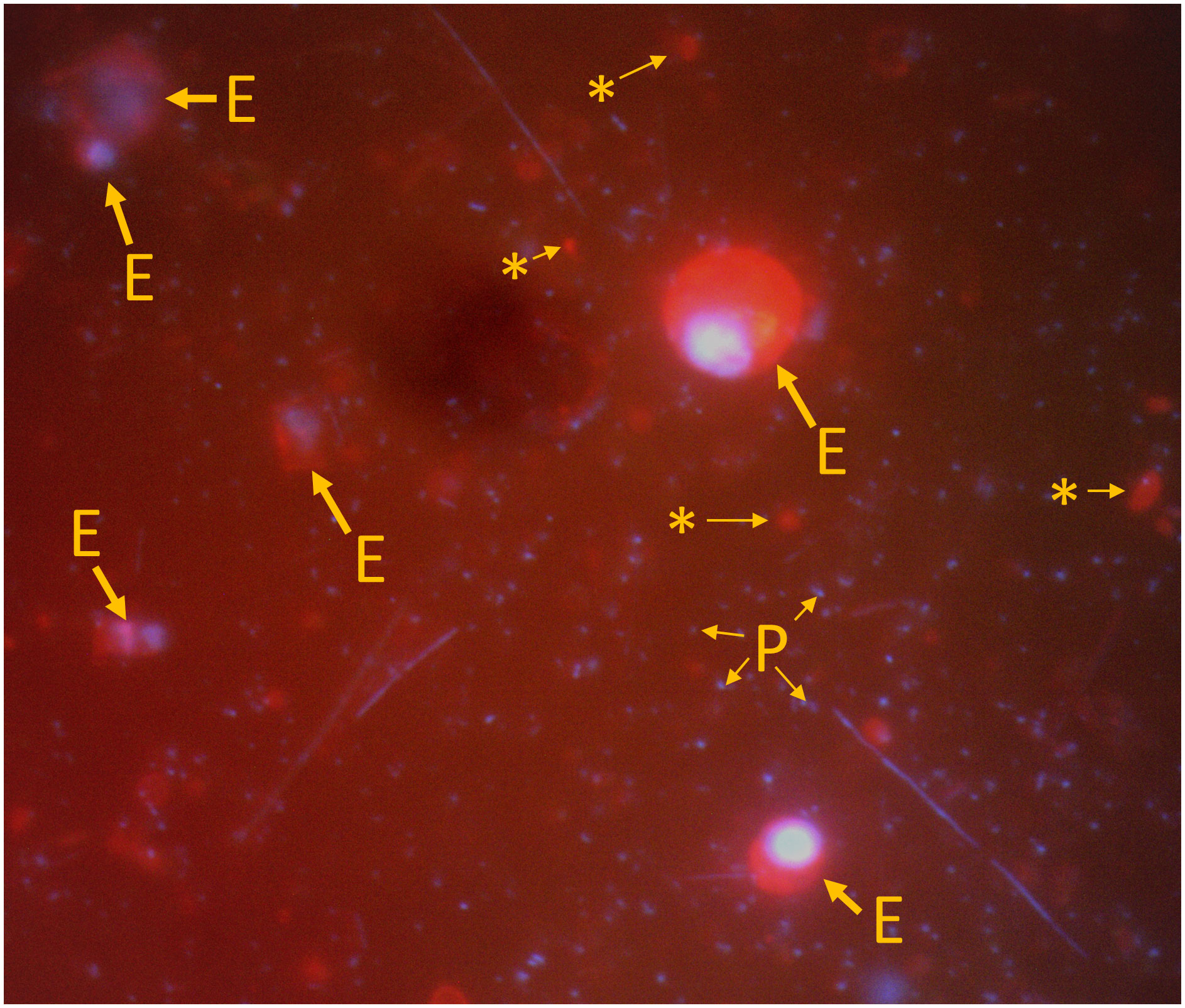
Figure 2 Example image for the enumeration of eukaryotes and biovolume estimates using DAPI (blue channel) and CellMask (red channel) dual staining. Images were each overlaid with 50% transparency. CellMask stains the cell membrane and thus allows us to better delineate the cell body for volume estimation. The smallest DAPI signals correspond to prokaryotes (P). Some cells are clearly eukaryotes containing a nucleus (E). Others are also stained with CellMask but lack a nucleus (*) and were considered detritus.

Results

During both cruises, we traversed a wide gradient in salinities ranging in sigma-t from ~8 to 25 (Figure 3). During the April 2018 cruise, the front of the Chesapeake Bay plume was clearly visible as an abrupt change in surface ocean color. We straddled this front with CTD stations #3 and #4, which while only 58 m apart produced distinct sigma-t profiles (Figure 3A). During the second transect cruise (2019), open ocean water with sigma-t values above 20 was present below the plume water (Figure 3B).

Figure 3

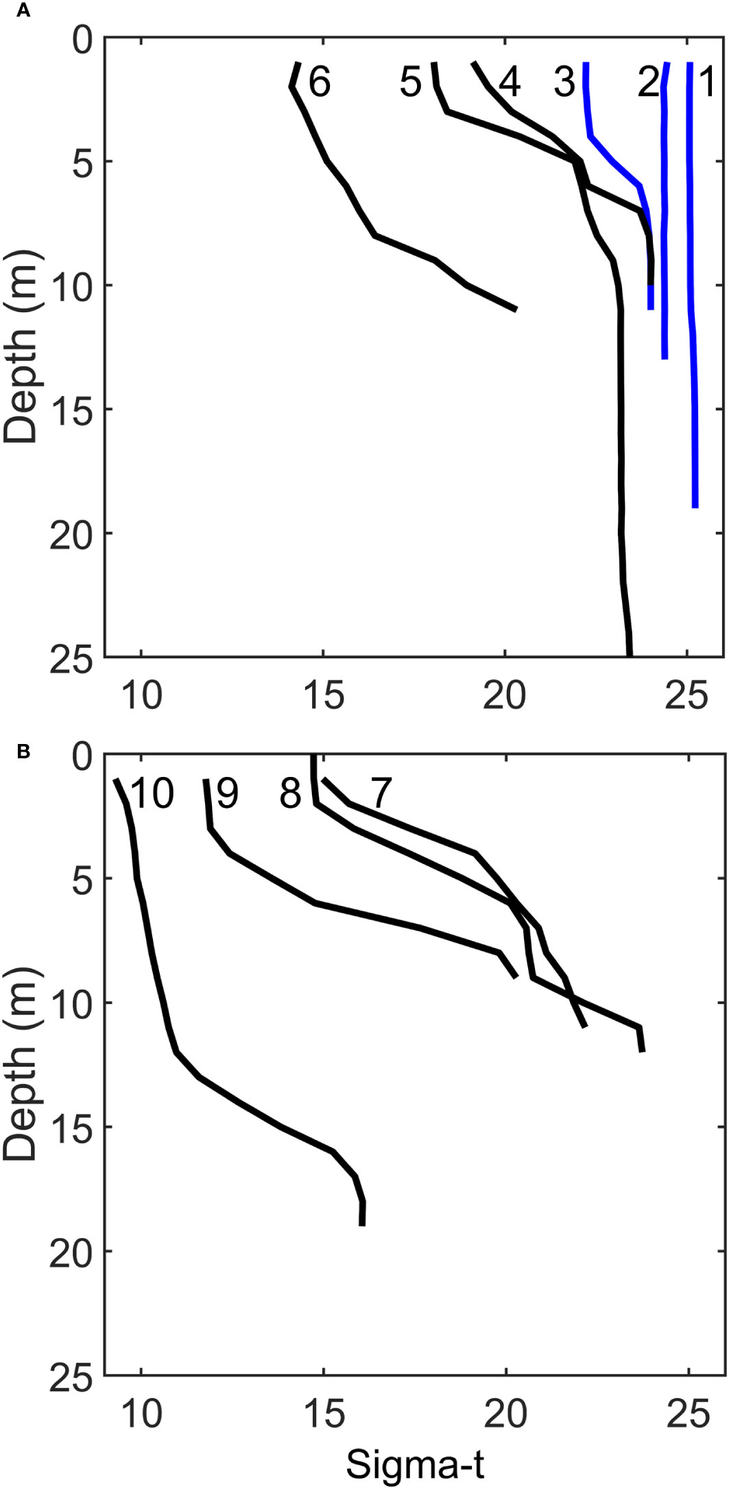
Figure 3 Sigma-t values of the six stations in April 2018 (A), and four stations in June 2019 (B). Blue lines indicate stations outside the Chesapeake Bay plume.

During the 2018 expedition, the ATP extraction protocol for polycarbonate filters was not fully developed, and we therefore only report the total ATP fraction (unfiltered “whole water”) from that cruise. During the 2019 expedition, liquid nitrogen and an incubation in a boiling-water bath was added to arrive at the highest extraction efficiencies using hot water (Bochdansky et al., 2021). The dissolved ATP fraction was determined for the 2019 cruise and was 12.5% (SD = 6%, n = 20) of total ATP. This percentage was not correlated to any of the environmental indicators (e.g., sigma-t, chlorophyll fluorescence). We conclude therefore that dissolved ATP was only a small fraction of total ATP.

Biomass based on microscope counts of prokaryotic microbes in both expeditions were significantly correlated with environmental indicator variables across the trophic gradient from open coastal water to the estuarine system (Figure 4, Table 2). The same bacterial and eukaryote carbon numbers were consistently less correlated with these variables than ATP (Figures 4, 5), which in turn had higher Pearson product moment correlation coefficients of 0.62 with chlorophyll fluorescence, -0.77 with density, and 0.81 with beam attenuation (Figure 4). Neither the biomass estimates from the microscopic examination of the Lugol’s samples from 2018, nor the estimates using cell volumes based on CellMask membrane stain were significantly correlated with pATP values or any of the environmental variables (Table 2). Whole-water ATP, however, was significantly correlated with the microscopically estimated eukaryotic carbon in the April 2018 data set when using a cell counts and fixed per cell carbon values (Table 2).

Figure 4

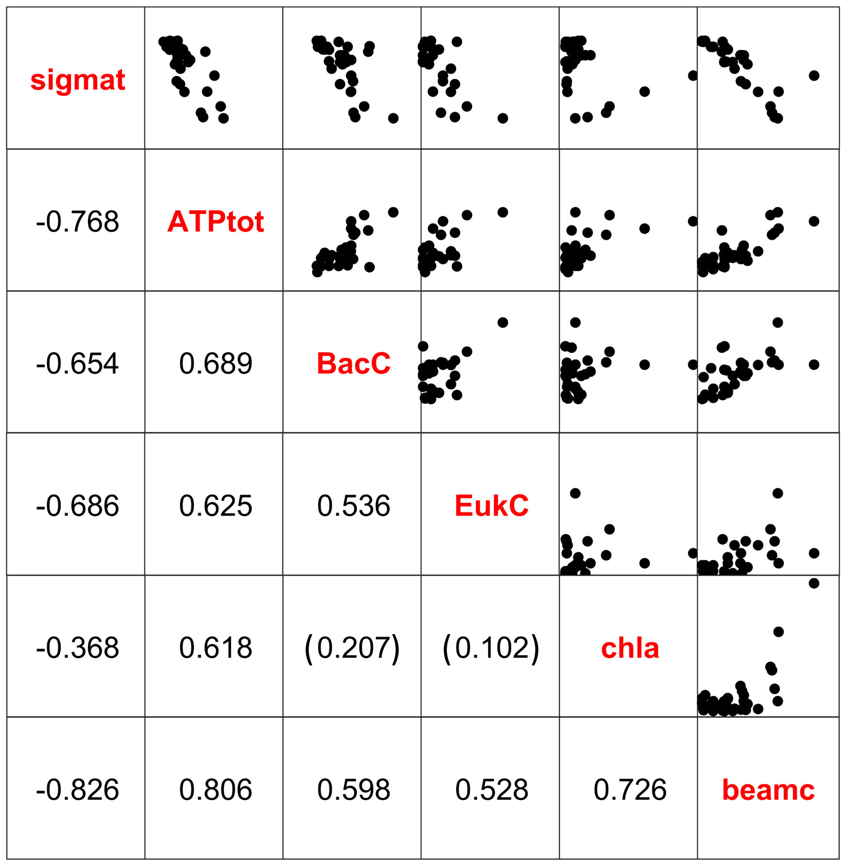
Figure 4 Pearson product moment correlation coefficients and scatter plots of sigma-t (sigmat), total ATP (ATPtot), bacterial carbon (BacC), eukaryotic carbon (EukC), chlorophyll fluorescence (chla), and beam attenuation (beamc) during the April 2018 research expedition. All correlations were significant at the α = 0.05 level except as indicated by parentheses.

Figure 5

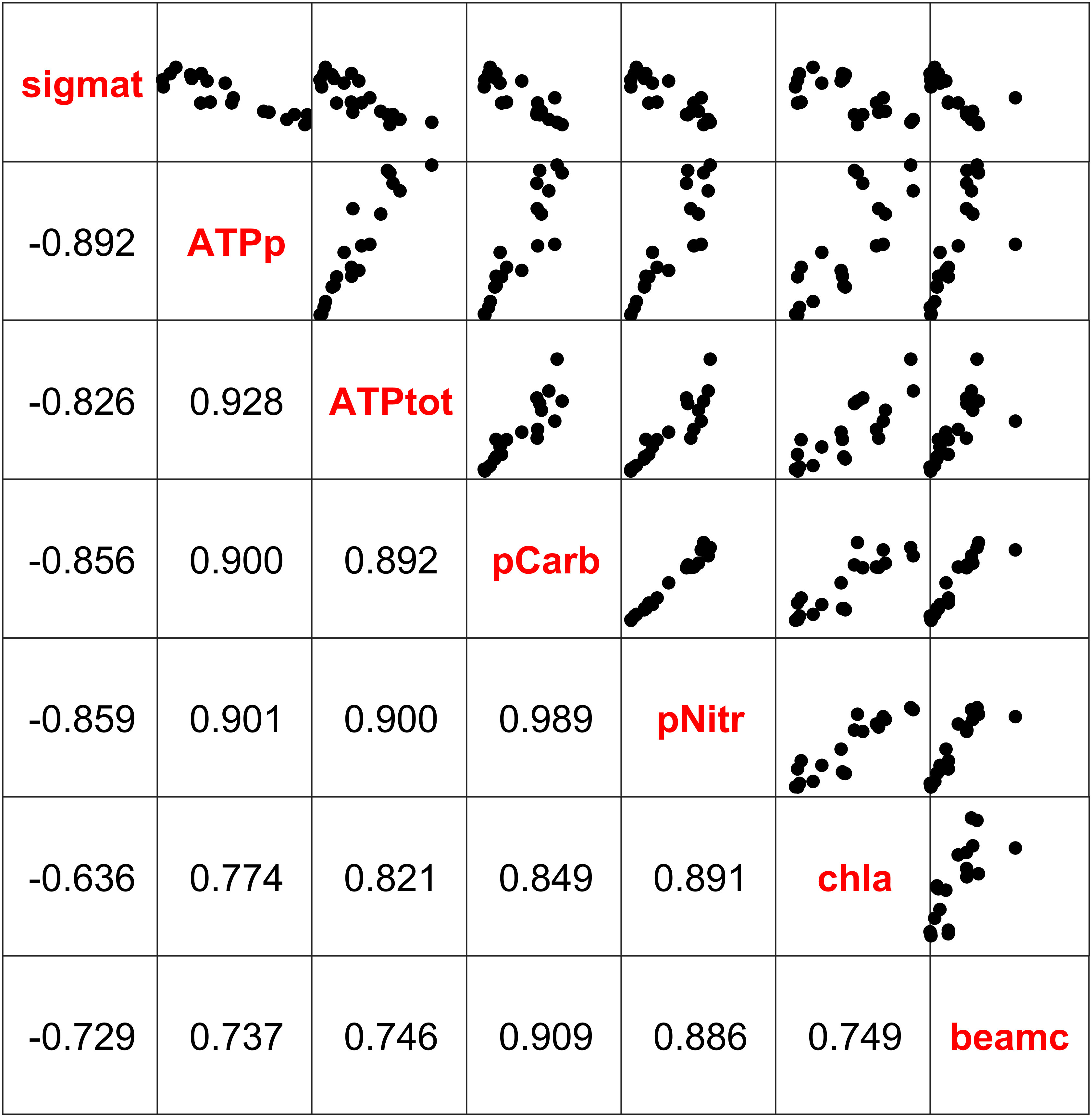
Figure 5 Pearson product moment correlation coefficients and scatter plots of sigma-t (sigmat), particulate ATP (ATPp), total ATP (ATPtot), particulate organic carbon (pCarb), particulate organic nitrogen (pNitr), chlorophyll fluorescence (chla), and beam attenuation (beamc) during the June 2019 research expedition. All correlations were significant at the α = 0.05 level.

Table 2

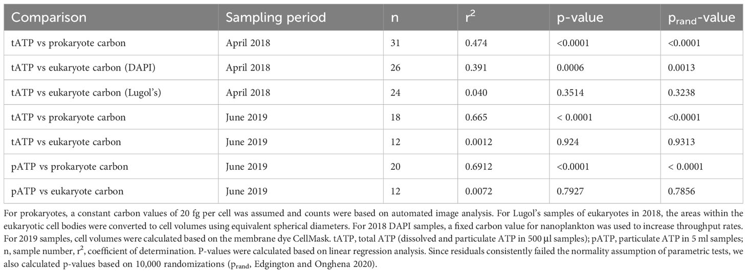
Table 2 Relationship between biomass estimates from microscopic observations and ATP values during the two cruises.

In the 2019 cruise, particulate carbon, nitrogen, and chlorophyll were highly correlated with ATP and each other, with coefficients ranging from 0.89 to 0.99 (Figure 5). Both particulate and total ATP were also significantly (at α = 0.05) and highly correlated with density (sigma-t), chlorophyll a, and beam attenuation (Figure 5).

Relationships between total ATP and chlorophyll a in the 2018 and 2019 transects show considerable overlap but have significantly different slopes (ANCOVA, homogeneity of slopes, n = 56, F = 4.34, p = 0.0423, Figure 6). This p-value is close to the criterion of α = 0.05, and we recalculated the p-value using a randomization test with 10,000 iterations to be p = 0.0449 (Edgington and Onghena, 2007). The confidence in a significant difference in slopes is therefore low and primarily driven by two high chlorophyll a values during the 2018 cruise (Figure 6).

Figure 6

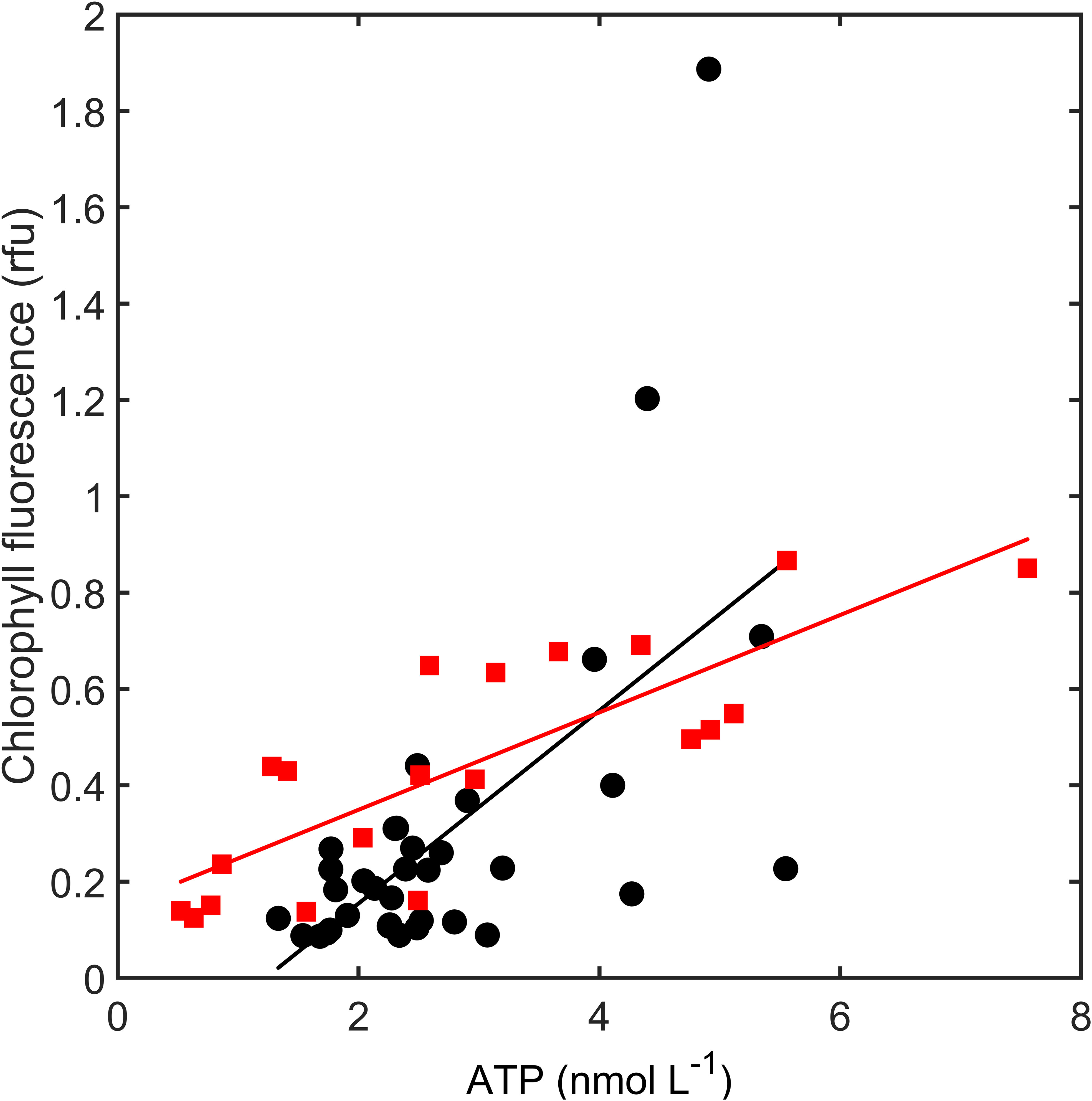
Figure 6 Chlorophyll fluorescence (relative fluorescence units, rfu) and ATP in April 2018 (black symbols) and June 2019 (red symbols). Linear regression 2018: y = -0.2463 + 0.2003 x (r² = 0.382, n = 35, F = 20.37, p< 0.0001); Linear regression 2019: y = 0.1011 + 0.1468 x (r² = 0.674, n = 20, F = 37.20, p< 0.0001).

There was a high correlation between POC and ATP values for both the total and particulate fraction (Figure 7). The relationship is close to linear, although a non-linear fit using a second-order polynomial slightly increased the explained variance (r²) and improved the residual pattern around the regression (Figure 7). Given the variance of the data, and the fact that both models are close in r², adoption of the curvilinear model with a higher level of parameterization is not fully justified. Despite the fact that blank values were subtracted for both ATP and carbon, the offset in the relationship between the two variables was considerable. Assuming a mass conversion of 250 from ATP to carbon (Holm-Hansen, 1973; Karl et al., 2022), the predicted live biomass in carbon values was ~15% at the lowest values offshore, increasing to ~30% at higher values inshore estimated from the regression model (Figure 7). Based on a sample-by-sample comparison between measures of particulate carbon and ATP values, and assuming a carbon-to-ATP mass ratio of 250, the range of ratios was 14–43% with an average of 27% (SD = 8.2%).

Figure 7

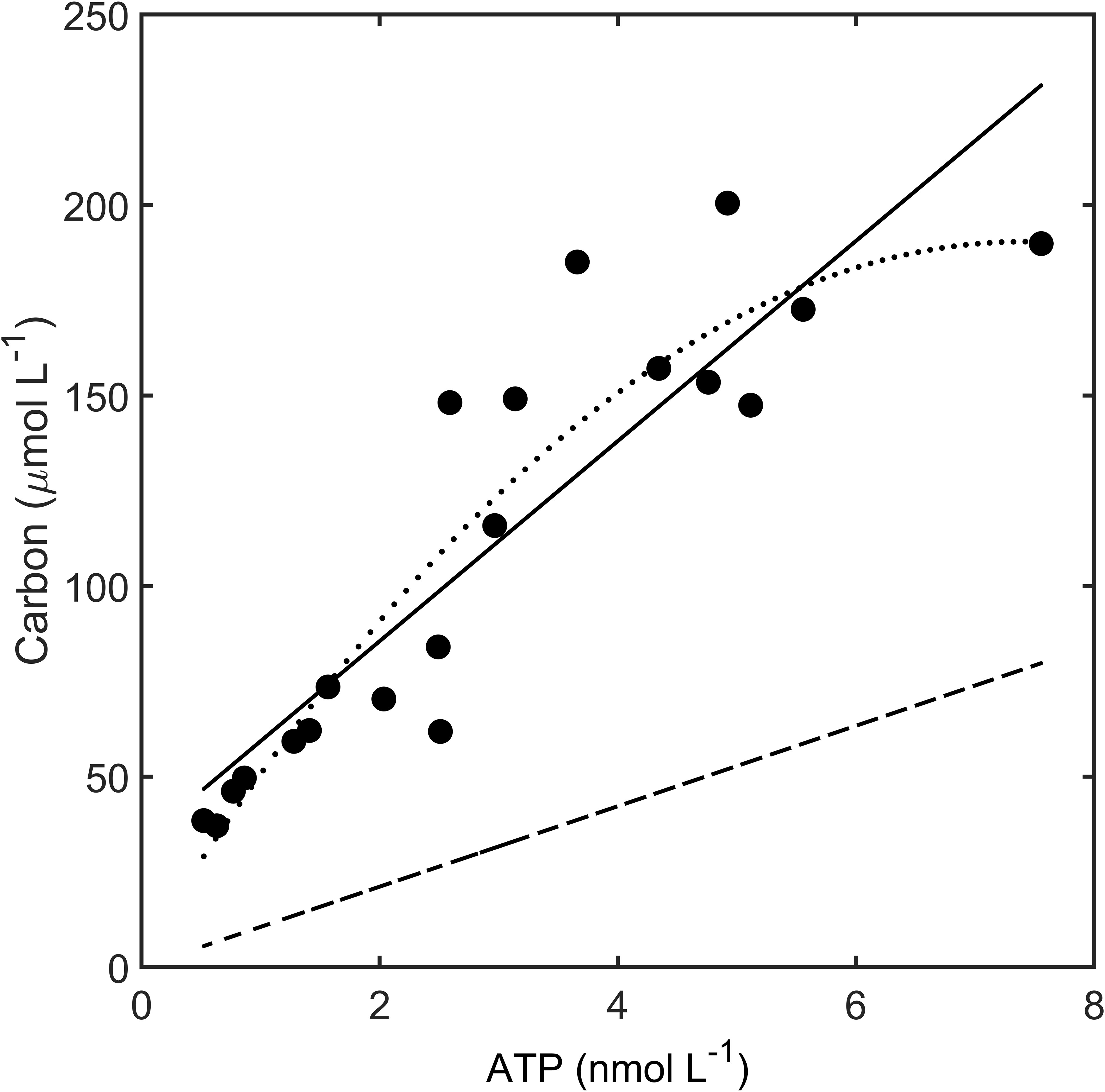
Figure 7 Relationship between total ATP and carbon during the June 2019 expedition (circles). Linear regression of carbon against ATP (solid line): y = 33.03 + 26.26 x, n = 20, r² = 0.797). Second-order polynomial (dotted line): 3.69 + 50.31 x - 3.389 x² (n = 20, r² = 0.856). Biomass carbon was predicted from ATP based on a mass conversion coefficient of 250 (dashed line).

Discussion

Methodological considerations

The data collected in this study are based on extractions with hot water after liquid nitrogen treatment (Bochdansky et al., 2021). While this extraction procedure yielded higher ATP values than the traditional method of boiling filters in a Tris buffer, a chemical extraction with phosphoric acid benzalkonium chloride (P-BAC) yielded slightly higher values still than the liquid-nitrogen hot-water extraction procedure (Bochdansky et al., 2021).

The literature on ballast-water monitoring using ATP as an indicator notes the use of several newer methods that promise even higher extraction efficiencies than the traditional method, due to mechanical and chemical (e.g., enzymatic) pretreatment (e.g., Lo Curto et al., 2018). The chemicals used in these kits are often proprietary, however, and the resulting ATP yields are inconsistent (Peperzak, 2023). For example, enzymatic pre-digestion using the LuminUltra kit shows a lower ATP yield than that of the P-BAC extraction (Welshmeyer and Kuo, 2016).

Our liquid-nitrogen hot-water extraction techniques reported here are within 20% of the maximum extractions attainable with P-BAC (Bochdansky et al., 2021). We also chose hot-water extraction as we also measured ATP in the dissolved fraction, and boiling water, liquid nitrogen, and a freezer were at hand, and the chemical extraction protocol was not fully developed at the time. In the future, and for routine measurements or the particulate ATP fraction only, we highly recommend using the P-BAC extraction procedure as it is efficient and quick, and P-BAC inactivates ATPases rapidly, so that samples do not need to be frozen if they are returned to the laboratory within a few hours.

Microscopic biomass estimations

While often used as the gold standard, microscopic determination of biomass has a variety of limitations, not least of which is that it is extremely labor-intensive when done correctly (e.g., Bradie et al., 2018). In our experiment, the high-throughput, automated analysis of bacterial numbers, and the manual counting of protist nuclei, applying a fixed carbon-per-cell assumption in both cases, resulted in a closer relationship to ATP and physical variables than the more detailed, time-consuming analysis based on individual cell numbers and volumes (Table 2). A simple reason for this discrepancy is that eukaryotic microbes are much less numerous than prokaryotes, thereby increasing the variance and decreasing the precision of the estimates. Cell volume estimates can only be reasonably performed on a small subset of organisms, resulting in high variability among the estimates obtained. Sample-to-sample variability in biomass, for example, may be greatly increased by the presence or absence of a few very large cells in individual samples that disproportionally contribute to biomass. On the other hand, higher throughput methods such as the automated counting of prokaryotes yield higher analytical precision. However, while counting millions of cells automatically increases precision, this method suffers from the fact that only a subset of microorganisms (i.e., prokaryotes) is assessed, and larger cells are left out. This is especially true in eutrophic systems, in shallow coastal and estuarine waters, where most of the biomass is bound in larger cell types such as dinoflagellates, diatoms, and ciliates, which are not accounted for in the prokaryote counts (Hobson et al., 1973; Cho and Azam, 1988; Laws et al., 1988; Verity et al., 1996b; Steinberg et al., 2001). Including eukaryote cells in the biomass estimates produces additional problems. Converting cell numbers to carbon is much more problematic for eukaryotic protists given their extreme ranges in cell size and shapes (Finlay, 2002). Picoeukaryotes are particularly difficult to enumerate as their cell sizes are close to those of prokaryotes, thus size fractionation with filters and genomic methods are used to estimate their diversity without enumeration (Jing et al., 2018). Fluorescence in in situ hybridization using universal eukaryote primers can be used for their identification and direct enumeration; however, this method suffers from cell losses during the preparation of the filters (Bochdansky and Huang, 2010; Morgan-Smith et al., 2011; Morgan-Smith et al., 2013; Bochdansky et al., 2017b).

In addition to problems with low statistical power, measurements of cell bodies of eukaryotic cells are inherently difficult to convert into biomass. As the shapes of cell bodies are only available in two dimensions, assumptions for the third dimension need to be made based on simple geometries when volumes are calculated. The path we chose here (i.e., the conversion from projectional area to volume) is more accurate than the conversion from two-dimensional shapes and does not assume rotational symmetry over the major axis (Hillebrand et al., 1999; Sun, 2003; Bochdansky et al., 2017a). Even with the application of a stain like CellMask, which specifically stains the cell membrane surrounding the cytoplasm, the cell body is often difficult to delineate (Figure 2).

Finally, heavy cell walls, cytoskeletons, and large storage vacuoles should arguably not be included in any measure of biomass. Yet skeletal and shell structures may substantially contribute to the volume of microbial cells as well as to their elemental and biochemical composition. Examples of skeletal structures include calcium carbonates in coccolithophorids (Paasche, 1968) and foraminifera (Jacob et al., 2017), cellulose skeletons in dinoflagellates (Taylor, 2006), silica skeletons in diatoms (Grønning and Kiørboe, 2020) and many rhizarians (Llopis Monferrer et al., 2020), leathery protein matrices found in the shells of tintinnids (Dolan, 2012), as well as the more obscure and inherently unstable strontium sulfate skeletons of acantharians (Beers and Stewart, 1970), to name just a few examples. Many microorganisms contain large vacuoles filled with water and salts, used for storage of nutrients or waste products, or to increase the rigidity of the cells (Schreiber et al., 2017). Diatoms, for instance, have long been known for their unusually large vacuoles that require distinct regression equations for the conversion of cell volume to carbon (Strathmann, 1967; Menden-Deuer and Lessard, 2000). By contrast, ATP is highly abundant and relatively constant in cytoplasm because of its function as a hydrotrope (Patel et al., 2017; Sarkar and Mondal, 2021) and consequently ATP primarily represents cytoplasm volume, excluding storage vacuoles and dead skeletal materials.

Systemwide comparisons of ATP

In general, records in the literature of a variety of environments are surprisingly consistent, despite the wide-ranging conditions and the numerous investigators involved (Table 3). Data can be ranked according to expected trophic positions with the deep sea at one extreme and eutrophic estuarine systems at the other (Table 3). Our ATP data fall well within the ranges expected for similar environments that have been sampled in the past (Table 3). The coastal ocean, the Chesapeake Bay plume, and the sample station in one of the tributaries span the range from moderately productive (coastal ocean, ~0.5 nM) to eutrophic (Elizabeth River, ~8 nM). The convergence of results in the context of environmental gradients is highly encouraging, especially given the fact that we have used a new simplified protocol (Bochdansky et al., 2021), while most other measurements were based on the original method (Holm-Hansen and Booth, 1966). Furthermore, Vosjan et al. (1987) used two different extraction methods—one based on a nucleotide-releasing substance and the other on a boiling Tris buffer—and found no systematic difference between the two approaches.

Table 3

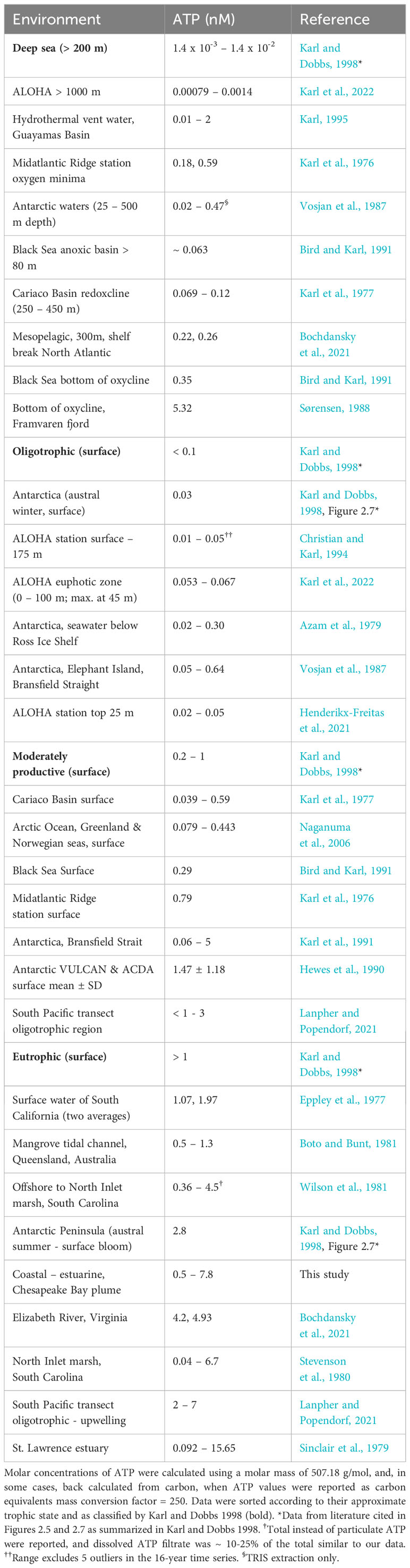
Table 3 Comparison of particulate ATP in estuarine and ocean environments.

The longest and most consistent record of ATP levels in any aquatic system is that of the Hawaiian Ocean Times Series station ALOHA, which has been taking samples since 1989 (Henderikx-Freitas et al., 2021, 2021). In a recent reanalysis of upper euphotic zone data at ALOHA, approximately 30% of POC was due to living biomass (Henderikx-Freitas et al., 2021; Karl et al., 2022). Importantly, assessment of biomass via ATP was consistent with the observed growth rates (Henderikx-Freitas et al., 2021), which provides an independent confirmation of the ATP-biomass method based on in situ physiological measurements. While the contribution of live biomass to total POC is high at the surface at station ALOHA, it decreases to only ~3% of total POC in the bathypelagic ocean (Karl et al., 2022).

Interesting patterns emerge from the intercomparison of environments (Table 3). Of the few measurements of ATP taken in estuarine and coastal environments, the highest values were found in the St. Lawrence estuary, with maximum values of ~16 nM (Sinclair et al., 1979). The North Inlet marsh system (near Georgetown, South Carolina) had ATP values very similar to the ones recorded here, ranging from 0.02 to 3.39 mg/m³ (μg/L) (0.04–6.7 nM ATP, using the conversion of 507.18 g mol^-1).

A noteworthy dynamic of the relationship between ATP-estimated biomass and POC was observed in a mangrove swamp in Queensland, Australia, where the proportion of live carbon changed drastically depending on the tidal state (Boto and Bunt, 1981). During slack tide, when organic matter settled to the bottom, biomass was a large portion of the total POC (45%–100%), while during strong resuspending currents, POC was dominated by detrital carbon, with only a small fraction (5–10%) composed of living microbes (Boto and Bunt, 1981). Since ATP values were not available, we digitized data from Figure 3 of the Queensland study, and back-converted the live carbon (“viable biomass”) to ATP using the authors’ mass conversion factor of 250 (Table 3). While detrital carbon fluctuated widely in this system, the biomass-carbon fraction remained surprisingly constant (Boto and Bunt, 1981). In situations of highly variable detrital carbon like these, any translation from POC to biomass will therefore always be problematic.

Azam et al. (1979) measured ATP levels in seawater below the Ross Ice Shelf, Antarctica, and concluded perhaps incorrectly that the values were close to the bathypelagic ocean. In fact, their values were much higher than deep-sea measurements and very close to the range reported later and measured independently for Antarctic surface waters by Vosjan et al. (1987) (Table 3). This again demonstrates little investigator bias in our compilation.

Another fascinating result of the intercomparison of ATP levels over a large range of marine ecosystems are the high values that are independent of photosynthetic production, such as those measured in oxyclines or in the nepheloid layer just above the benthos (Karl et al., 1976). This is consistent with high-biomass samples observed microscopically, and with the highest biomass of ciliates containing endosymbionic bacteria in oxyclines of the Black Sea, the Baltic Sea, and the Cariaco Basin (Sorokin, 1972; Karl et al., 1976; Fenchel et al., 1990; Taylor et al., 2006; Edgcomb and Pachiadaki, 2014). However, an increase in ATP biomass was not always observed in oxyclines (Devol et al., 1976) and further investigation is needed.

The observation that ATP mirrors environmental gradients better in our data than cell enumeration or cell volume estimations is a strong indicator that ATP is not only less time-consuming but also a better overall indicator of biomass. Whether ATP can be considered a “master variable in microbial ecology” (Karl and Dobbs, 1998) depends on how well we can further integrate the derived values into the framework of ecological models.

Calculating microbial carbon from ATP

Given the highly variable elemental composition of microbial cells (Sterner and Elser, 2002), on the one hand, and the low variance of plasma concentrations of ATP observed in a variety of organisms, on the other (Bochdansky et al., 2021, and references cited therein), it is worth resisting the impulse to reflexively convert ATP to carbon values. In fact, some cursory observations suggest that cellular nitrogen may be more closely related to ATP than cellular carbon (Bochdansky et al., 2021).

However, carbon is the most frequently used and universal currency in ecosystem models, and there is value exploring the relationship between ATP and carbon further. For an approximation of live carbon, the original mass conversion factor (grams to grams) of 250 continues to be the most useful (Holm-Hansen, 1973; Karl et al., 2022). Note that the Holm-Hansen (1973) conversion factor is based on mass conversions (1 g ATP = 250 g carbon). The molar conversion factor from moles of ATP to biomass in moles of carbon (e.g., in Table 3) is thus 10,566.25 (507.18*250/12). One of the few studies that have corroborated this conversion with live plankton in situ was by Paerl and Williams (1976), who arrived at a slope of 276 between carbon and ATP. This value is very close to our own estimates of 280 in a culture of Thalassiosira weissflogii (Bochdansky et al., 2021). However, many challenges exist surrounding the conversion of ATP into carbon, as previously detailed (Karl, 1980; Christian and Karl, 1994; Karl and Dobbs, 1998).

To obtain useful carbon-to-ATP ratio for microbes, cells have to be grown close to axenically (i.e., with only a negligible amount of bacteria present), and cultures need to be free of detritus such as accumulations of dead cells and extracellular organic material (Christian and Karl, 1994). There have been a few reports of deviations in carbon-to-ATP mass ratios, ranging from 150 to 400, with much of this variance being driven by extreme phosphorus limitation (Cavari, 1976; Karl, 1980; Hunter and Laws, 1981; Christian and Karl, 1994). While more data are needed to examine its effect on intracellular ATP levels, phosphorus limitation alone is relatively rare in marine systems, and where it does occur it is mostly co-limited by nitrogen and iron (Moore et al., 2013).

It is difficult to ascertain how much of the divergence in the C:ATP ratio seen by Hunter and Laws (1981) can be attributed to dead cells in the sample, and how much is due to a variable carbon-per-cell content independent of ATP (see discussion by Bochdansky et al., 2021). For instance, per-cell carbon values changed over a two-fold range in the diel cycle of phytoplankton (95–200 pg cell^-1 in Thalassiosira fluviatilis, i.e., T. weissflogii), while by contrast, the ATP-per-cell values only ranged from 0.75 to 0.95 pg cell^-1 (Hunter and Laws, 1981). The variable C:ATP ratios are thus more likely to be the result of variable carbon-per-cell values due to the accumulation of photosynthates during the light cycle.

The most desirable evidence for ATP concentrations in microbes would come from direct measurements in single cells in the field. However, these measurements were so far only possible in cultures and in large protists such as amoeba (Ueda, 1987). Single-cell ATP values were measured in an elegant fashion in cultured bacteria using Escherichia coli strains transformed with a vector containing an ATP indicator sequence (Yaginuma et al., 2015). A very distinct mode at ~1 mM was shown, albeit with some cell-to-cell variability (Yaginuma et al., 2015). The cellular ATP concentration of approximately 1 mM is consistent with a wide range of cell types, especially given that cell constituents other than cytoplasm contribute to the measured cell volumes (Bochdansky et al., 2021).

Live versus dead (detrital carbon) carbon

To better model ecosystem processes it is important to understand the contribution of living and non-living POC (Kharbush et al., 2020; Scheffold and Hense, 2020), as organisms are the “active ingredients” in the ocean (i.e., those that mediate processes). Lack of an ability to separate detritus from organisms, and the fact that detritus does not exist without attached microorganisms, has led to the use of identifiers such as “biodetritus” (Odum and de la Cruz, 1963; Smetacek and Hendrikson, 1979; Christian and Karl, 1994). This is a justified capitulation to methodological difficulties in separating microbes from non-living particulate matter based on microbial cell enumeration. Even if cells could be counted accurately in complex organic matrices, the big question would remain as to how many cells are alive, and how many are dead cell debris or “ghosts” (Zweifel and Hagstrom, 1995). The use of ATP instead of cell counts greatly alleviates this problem.

The contribution of live cells to POC varies greatly depending on the study (Hobson et al., 1973; Banse, 1977; Sinclair et al., 1979; Laws et al., 1988; Cho and Azam, 1990; Andersson and Rudehäll, 1993; Steinberg et al., 2001). Some of the observed variance is environmentally driven, such as due to nutrient availability, but there are almost certainly methodological effects as well. Microscopic enumeration, for example, almost entirely neglects a large pool of transparent particles that are large enough to be trapped by GF/F filters and thus contribute to total POC (Bochdansky et al., 2022). These particles typically require separate staining with Alcian blue or Coomassie Brilliant Blue to be accurately enumerated (Alldredge et al., 1993; Long and Azam, 1996).

The scope of this study prohibits a comprehensive review on this topic but all components (carbon, nitrogen, chlorophyll, etc.) vary widely among major compartments such as detritus, prokaryotes, eukaryotes, and heterotrophic plankton (Banse, 1977; Sinclair et al., 1979). Chlorophyll is a very poor predictor of carbon even for phytoplankton because of seasonal photo-acclimation (e.g., North Pacific Transition Zone) (Britten, 2022) and light acclimation in the deep chlorophyll maximum (Cullen, 2015). Global models in combination with satellite data suggest that phytoplankton carbon as a percentage of POC is highest in tropical and subtropical regions, with a range of 30–70%, and lower in high-latitude regions at 10–30% (Arteaga et al., 2016). Open ocean bacteria, on the other hand, are reported to contribute typically 15–25% of POC (Kharbush et al., 2020, and references cited therein). Combining these estimates of bacterial and phytoplankton carbon would add up to more than 100% of POC, however. This clearly contradicts estimates of 50–90% of detrital carbon (see below) and exemplifies the problems of estimating biomass whenever microscopic analysis or chlorophyll are used as metrics for biomass.

A 10:1 mass ratio is often assumed between detritus and live plankton, respectively (Hobson et al., 1973; Cauwet, 1977; Karl and Dobbs, 1998; Volkman and Tanoue, 2002), but this ratio is greatly influenced by a variety of factors such as methodology, the environment, trophic status, seasonality, and depth. Detritus in the water column can also increase as a result of accumulating fecal material in the water column during zooplankton blooms (e.g., by tunicates, as noted by Pomeroy and Deibel, 1980).

High biomass-to-POC ratio estimates come from the surface environments of subtropical gyres such as the Sargasso Sea and the North Pacific subtropical gyre. Live biomass has been reported to represent 55% of POC in the spring and 24% in the summer in the Sargasso Sea (Caron et al., 1995), and 26–42% of POC at the surface of the North Pacific Subtropical Gyre (Henderikx-Freitas et al., 2021). Values from the Sargasso Sea were based on microscope counts, while in the North Pacific Subtropical Gyre, estimates were based on ATP. In the same regions, biomass decreases much more rapidly with depth than POC, leaving only ~3% of carbon for biomass at depths > 3,000 m (Karl et al., 2022). In the North Pacific Ocean and the Bering Sea, living biomass measured using ATP values ranged from 5% in the subtropical Pacific to 23% of POC in the Bering Sea (Yanada and Maita, 1995).

Our own estimates of live biomass as a percentage of POC range from 15% to 40% (Figure 7), and fit well into the ranges reported for similar systems. For instance, in a detailed analysis of detrital carbon, live carbon, and chlorophyll in Virginia shelf water, it was determined that 20–75% was detrital carbon, translating into a respective range of 80–25% live carbon (Verity et al., 1996a). In the Kiel Bight, detrital carbon was estimated to range from 25% to more than 75% of POC (indicating live proportions of 75–25%, respectively) with the higher values due to seasonal resuspension of detrital material from the benthos (Smetacek and Hendrikson, 1979). In the Baltic Sea, the percentage of detrital contribution ranged seasonally from 63% to 94% of POC (i.e., 37–6% live carbon) (Andersson and Rudehäll, 1993). The contribution of live carbon in the Baltic Sea was 8% in the wintertime, rising to 49% during the spring bloom, with biomass values also based on ATP (Andersson and Rudehäll, 1993).

In a transect south but not far from our study site, the relative number of metabolically active bacteria was measured through the intracellular accumulation of formazan reflecting active respiration (Sherr et al., 2002). POC increased moving from offshore to inshore stations, albeit at lower values as the region off Cape Hatteras is more oligotrophic and far outside the Chesapeake Bay plume. Bacterial numbers approximately doubled from offshore to inshore areas, and to a greater degree in March than in July, reflecting higher POC in the water column in the spring (Sherr et al., 2002). In contrast, POC increased more than three-fold in the same gradient. The authors also determined the proportion of metabolically active cells attached to detritus was strikingly higher than in whole-water samples (Sherr et al., 2002). In our case, with a larger gradient and higher POC values overall, ATP values ranged approximately seven-fold over the gradient we observed, while POC increased five-fold.

The higher percentage of live bacteria where there is a higher abundance of detritus matches our observations. The intercept and the slope in the relationship between particulate carbon and ATP tell two distinct but congruent stories (Figure 7). The high intercept reflects the fact that there is a large proportion of non-living material in the mesotrophic offshore and coastal regions. This fraction decreases as a percentage of POC in the gradient from the open ocean to the estuary as the higher nutrient concentration promotes phytoplankton growth, which is also reflected by the high correlation between chlorophyll fluorescence and ATP (Figure 6). By contrast, the slope of live carbon [i.e., carbon estimated on the basis of ATP, dashed line in Figure 7)] is shallower than it is for total particulate carbon, which indicates a higher proportion of detrital carbon at higher total POC (Figure 7). This is consistent with a higher level of allochthonous material such as decaying plant material from river runoff (Newell, 1984).

Conclusions

Overall, the question of how well ATP represents live material in the water remains. It is highly difficult to make this determination in the field, where ATP values per plasma volume cannot be readily assessed. Even so, most of the existing evidence points towards a high consistency between particulate ATP and live matter. From the open ocean to the shore, ATP levels are closely correlated with other metrics associated with increases in biomass, such as chlorophyll a, turbidity, and carbon.

It has been demonstrated in cultures that although ATP values per cell may vary to a small extent, other cell constituents (e.g., carbon, chlorophyll a) change even more, which in turn means that ATP is the more consistent and conservative metric of biomass. Using a constant conversion from ATP to carbon, we also observe a highly plausible pattern in the detritus-to- living material ratio that is very close to many other methods, is consistent with trends pointing in similar directions, and concurs with absolute values that fall into the ranges of data found in the literature.

Lastly, there is a theoretical basis for a constant ATP-to-cytoplasm volume ratio, based on the principle that cells require a homeostatically controlled concentration of ATP as a hydrotrope. All this evidence is encouraging, as a more detailed system-wide analysis of ATP will enable us to further decipher the complex interplay of the living and non-living carbon pools in aquatic systems. It would therefore be useful to introduce ATP as a standard metric of microbial biomass into future monitoring of aquatic systems.

Data availability statement

The datasets presented in this study can be found in online repositories. The names of the repository/repositories and accession number(s) can be found below: Biological & Chemical Oceanography Data Management Office: https://www.bco-dmo.org/project/917950.

Author contributions

ABB: Conceptualization, Data curation, Formal Analysis, Funding acquisition, Investigation, Methodology, Project administration, Supervision, Validation, Visualization, Writing – original draft, Writing – review & editing. AAB: Data curation, Investigation, Writing – original draft, Writing – review & editing. JC: Data curation, Investigation, Writing – original draft, Writing – review & editing. AS: Data curation, Investigation, Writing – original draft, Writing – review & editing. NW: Data curation, Investigation, Writing – original draft, Writing – review & editing.

Funding

The author(s) declare financial support was received for the research, authorship, and/or publication of this article. This study was funded by the National Science Foundation, awards # 1851368 and 2319114 (Divisions of Ocean Sciences, Chemical and Biological Oceanography). AAB, JC, AS, and NW were supported by the National Science Foundation through a Research Experience for Undergraduates Site Award (OCE 1659543) to H. Rodger Harvey and Katherine Filippino.

Acknowledgments

We thank the crew of the R.V. Slover (Old Dominion University) for their assistance during sample collection and Peter Bernhardt (laboratory of Margaret Mulholland, Old Dominion University) for conducting the POC & PON analyses.

Conflict of interest

The authors declare that the research was conducted in the absence of any commercial or financial relationships that could be construed as a potential conflict of interest.

Publisher’s note

All claims expressed in this article are solely those of the authors and do not necessarily represent those of their affiliated organizations, or those of the publisher, the editors and the reviewers. Any product that may be evaluated in this article, or claim that may be made by its manufacturer, is not guaranteed or endorsed by the publisher.

References

Alldredge A. L., Passow U., Logan B. E. (1993). The abundance and significance of a class of large, transparent organic particles in the ocean. Deep Sea Res. Part Oceanogr. Res. Pap. 40, 1131–1140. doi: 10.1016/0967-0637(93)90129-Q