
94% of researchers rate our articles as excellent or good
Learn more about the work of our research integrity team to safeguard the quality of each article we publish.
Find out more
ORIGINAL RESEARCH article
Front. Mar. Sci., 19 January 2024
Sec. Marine Fisheries, Aquaculture and Living Resources
Volume 11 - 2024 | https://doi.org/10.3389/fmars.2024.1243954
 Ernesto Carrella1
 Joseph Powers2*
 Steven Saul3Richard M. Bailey1
 Nicolas Payette1
 Katyana A. Vert-pre3Aarthi Ananthanarayanan2
 Michael Drexler2Chris Dorsett2
 Jens Koed Madsen4
Many of the world’s fisheries are “data-limited” where the information does not allow precise determination of fish stock status and limits the development of appropriate management responses. Two approaches are proposed for use in data-limited stock management strategy evaluations to guide the evaluations and to understand the sources of uncertainty: rejection sampling methods and the incorporation of more complex socio-economic dynamics into management evaluations using agent-based models. In rejection sampling (or rejection filtering) a model is simulated many times with a wide range of priors on parameters and outcomes are compared multiple filtering criteria. Those simulations that pass all the filters form an ensemble of feasible models. The ensemble can be used to look for robust management strategies, robust to both model uncertainties. Agent-based models of fishery economics can be implemented within the rejection framework, integrating the biological and economic understanding of the fishery. A simple artificial example of a difference equation bio-economic model is given to demonstrate the approach. Then rejection sampling is applied to an agent-based model for the hairtail (Trichiurus japonicas) fishery, where an operating model is constructed with rejection/agent-based methods and compared to known data and analyses of the fishery. The usefulness of information and rejection filters are illuminated and efficacy examined. The methods can be helpful for strategic guidance where multiple states of nature are possible as a part of management strategy evaluation.
Stock assessment models are used in fisheries analysis to determine status of a fish population relative to management criteria and to evaluate the change in status in response to management measures (Quinn and Deriso, 1999). The models are based on data obtained from the fishery, data obtained independent of the fishery and an underlying model (understanding) of the relationships of growth, mortality and reproduction. There is a wide continuum of models being implemented based on the availability of data and the management objectives that are being addressed. However, the central theme is that some parameters of the model are statistically estimated based on the data observations, other parameters are assumed based on prior knowledge and the uncertainty (probability distributions) of both are evaluated to the extent feasible. The methods to do this vary with data availability, but the ultimate goal is to provide estimates of management quantities, the uncertainties associated with those quantities and to provide advice on feasible policies for achieving management objectives. The latter activity, collectively called management strategy evaluations (MSEs) is the process of constructing (conditioning) an operating model of basic understanding of stock and fishery dynamics, to explore different management strategies in the face of uncertain scenarios and to evaluate performance metrics through projections, looking for strategies that are robust to uncertainty and which achieve acceptable tradeoffs between those performance metrics (Punt et al., 2016; Miller et al., 2019). The focus of this paper is on methods to develop MSES for fisheries which are data-limited.
Data-limited fisheries are ubiquitous and often are important components of the fisheries economy (Prince and Hordyk, 2018). Thus, recent research has addressed methods which can be used in data-poor fisheries (Carruthers et al., 2014; Hordyk and Carruthers, 2018; Dowling et al., 2022; Carruthers et al., 2023). While inadequacies of management advice resulting from the lack of data are not solved by modeling alone, data-limited MSEs can be designed to appropriately use the data that are available and to organize the results so that they can be cogently provided in terms that are useful for management. To that end, two approaches are proposed herein for use in data-limited MSEs. The approaches are: 1) rejection sampling methods for conditioning operating models for data-limited MSEs and 2) the incorporation of more complex socio-economic dynamics into that conditioning and also into the MSE projections using agent-based models that depict fishery socio-economic behavior of individuals and/or vessels on a daily basis. These methods may be viewed as adding to the continuum of modeling approaches and procedures for providing MSEs for data-limited fisheries (Dowling et al., 2022; Carruthers et al., 2023).
This manuscript is organized into a short explanation of rejection sampling methods, followed by a simple artificial example of suing rejection-sampling in conditioning an operating model based on a difference equation bio-economic model. Then rejection sampling is applied with agent-based modeling (Bailey et al., 2018) to the Bungo Channel Usuki troll fishery for hairtail (Trichiurus japonicas). This fishery was chosen as an example because of the unique documentation of stock assessment (Watari et al., 2017), socio-economics and initial MSEs of the fishery (Makino et al., 2017) and technical fishery operations (Hirose et al., 2017). Given this documentation, the hairtail fishery would not be considered data-limited. However, for this example Bungo Channel Usuki fishery is modeled as if it were data-limited and then results compared to the original documentation of Watari et al. (2017); Makino et al. (2017) and Hirose et al. (2017). By doing so, the usefulness of the agent-based approach and rejection filters are illuminated and the efficacy of the approach is examined.
Rejection sampling methods are used with models encompassing multiple parameters and, also, generic observation data or knowledge such as perceptions of catch and abundance history. The model simulates the dynamics of, for example, a fishery and stock abundance providing outputs. These outputs are matched with generic observations of the fishery. Those outcomes that are inconsistent with the limited observation data are rejected and the simulations remaining allow conclusions to be drawn that are more robust to misspecification. An ensemble can be built using rejection sampling (see chapter 14 in Russell and Norvig, 2009; see also “rejection filtering” in Hartig et al., 2011). At its core this simply means running the model many times with random parameters and rejecting all runs that do not match the data that was observed. If priors on the parameter space are provided, the resulting ensemble is the Bayesian posterior of all the “close enough” fisheries (this is the rejection approximate Bayesian computation of Beaumont et al., 2009. Beaumont et al., 2002). If priors are not provided, the ensemble can still be used to look for robust policies (those that work unanimously for every member of the ensemble) or can be split into groups to gain a better understanding of which policies work when (scenario-based uncertainty). This can be useful for strategic guidance where multiple states of nature are possible and is the basic goal of MSEs.
Rejection sampling (also under the name of rejection filtering) is popular in ecology as operationalization of pattern-oriented modeling (Grimm et al., 2005). Rejection sampling is also at the basis of the “ensemble ecosystem” approach of Baker et al. (2017) who generated a large set of qualitative Lotka-Volterra models and rejected those that did not match a set of known responses to shocks. Rejection sampling was also implicit in the Catch-MSY method (Martell and Froese, 2013; note Maximum Sustainable Yield is referred to as MSY). Rejection sampling can be structured such that the history and parameter combinations can be used to generate outcomes that are the result of simulated policy shocks across all accepted ensemble sets to look for patterns and vulnerabilities, i.e. MSEs (Carruthers et al., 2014; Hordyk and Carruthers, 2018). Rejection sampling requires no likelihood function. That feature allows matching of models with data that would otherwise be hard to use, in particular qualitative or socio-economic observations. Therefore, more complex socio-economic dynamics can be implemented through agent-based models for use in MSEs. This is not a substitute for data and more statistical assessment methods. However, it is a framework for simulating the fishery based on a large ensemble of unknowns and then evaluating the results in a consistent manner.
Start with a set of k pieces of evidence . The ei might be quantitative evidence like “catch this year is 1000 mt” or qualitative like “abundance this year is lower than it was 10 years ago”. Assume there is a model (simulation) that uses n parameters to generate synthetic evidence . Define a set of k filters, one for each item of evidence, ; these are predicate functions returning true if for some aspect of the evidence, the predicted is “close enough” to the real observed one E. The definitions of filters may be statistical if the evidence warrants it, effectively turning this into an indirect inference problem (Gourieroux et al., 1993). The filters may also be vague and more anecdotal.
The rejection sampling algorithm is implemented as follows:
Draw a set of random model parameters from prior distributions .
Run a simulation to generate set of synthetic evidence
Reject that simulation if at least one filter returns false (i.e., is not “close enough” to true)
This loop is repeated until the computational budget is exhausted. (Note that in many fisheries applications computational time is not a major issue. However, this is discussed further in the context of the hairtail example later in this paper.) The remaining simulations represent a plausible outcome based on the prior knowledge (distributions) of the parameters and the knowledge (filters) rejecting implausible evidence.
The ensemble of accepted simulations can be used to accomplish three analytical tasks. First, the individual effect of each piece of evidence and its associated filter on the distribution of parameters or outcomes of the model can be examined. Second, management policies can be simulated on the whole ensemble to examine their likely outcomes and uncertainties. Third, one can examine the evolution of the posterior distribution of parameters as the number of simulations accumulate to identify stopping criteria for the rejection sampling as a whole.
The bioeconomic model of Seijo et al. (1998) is presented here as a simple illustrative example, where a fish stock exhibiting logistic growth is targeted by vessels whose number change annually in proportion to profits:
where Bt is the biomass in year t, Yt is the catch in year t and ft is the effort in number of vessels. Other parameters and their prior distributions are defined in Table 1. Uniform prior distributions for each parameter were chosen and then using these priors and three conditions or filters, the rejection sampling process was implemented.
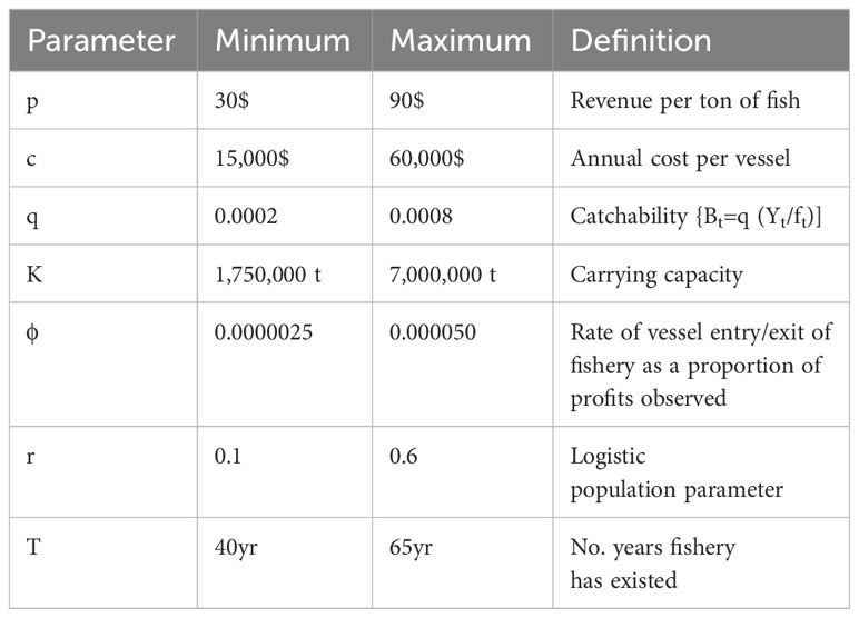
Table 1 Maximum and minimum values for uniform prior distributions for the parameters of Equation 1 [chosen from values in Table 2.1 in Seijo et al. (1998)].
The filters were conditioned on three pieces of information: 1) Catch filter: the landings in the current year were between 10,000 and 15,000 t; 2) Profit filter: the current fishery is not profitable; and 3) CPUE filter: catch-per-unit effort (CPUEt=Yt/ft) was higher ten years ago than it is currently. These, rather loose, criteria were translated into filters for Equation 1 and the rejection sampling algorithm was applied.
One million parameter sets were drawn from their uniform priors When the current catch filter was applied the accepted number of simulations was reduced to 10718. When the current catch and current profit filters were applied, then the accepted number of simulations was further reduced to 4427. Finally, when all 3 filters were imposed then only 3,435 simulations passed, an acceptance rate of 0.3%. Each simulation generated a time series of biomass, catch and effort based on the selected parameters starting at T years before and ending at what is referred to as the “current” time. The impact of the filters on MSY (MSY=rK/4, Figure 1) and Depletion (current biomass relative to the biomass at the beginning of the fishery (BCurrent/K), Figure 2) was examined by looking at the posterior probability distributions using all 106 simulations (the priors) and then the results sequentially when only the catch filter was passed; then results if both the catch and profit filters were passed and then finally if all three filters were fulfilled. The mean MSY from the priors was 383,000 t. The mean shifted to 236,000 twhen the catch filter was imposed, then to 225,000 t when the catch and profit filters were imposed and remained at 225,000 t when all filters were imposed (Figure 1). The depletion distribution arising from the priors was bimodal with a mean depletion of 0.41. Imposition of the catch filter did not alter the mean or the bimodality (Figure 2). However, the additional profit filter (and subsequently the CPUE filter) reduced mean depletion to 0.11 and effectively eliminated the bimodality.

Figure 1 Relative frequency distribution (Density) of MSY estimates from 106 simulations: (A) using all 106 simulations generated from the Priors; (B) using only simulations that passed the Catch filter; (C) using simulations passing the Catch and profit filters; and (D) using simulations that passed all three filters (Catch, profit and CPUE).
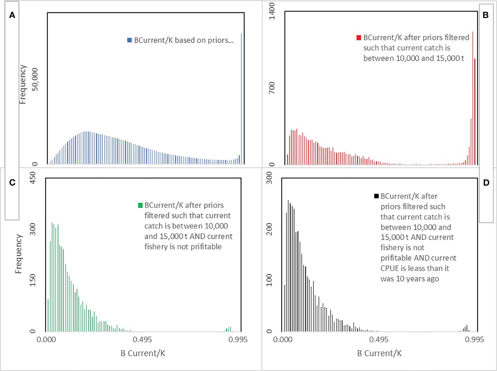
Figure 2 Relative frequency distribution (Density) of current depletion (Bcurrent/K) from 106 simulations: (A) using all 106 simulations generated from the Priors; (B) using only simulations that passed the Catch filter; (C) using simulations passing the Catch and profit filters; and (D) using simulations that passed all three filters (Catch, profit and CPUE).
The rejection sampling phase is a mechanism to condition an “operating model”. The operating model is an expression of basic understanding of the biological and fishery dynamics of the stock and fishery. It is understood that there is uncertainty in that understanding, as exemplified by the broad distribution of key quantities in this example (e.g. Figures 1, 2). In this case, the operating model is Equation 1 with the accepted (filtered) parameter set. The operating model generated a time series of biomass, catch and effort from the beginning of the fishery to “current” time for each of the 3435 simulations and the parameter set for each simulation. The operating model can then be used to explore management strategies, evaluate scenarios where knowledge is uncertain (such as parameter uncertainty or non-stationarity of parameters or models) and the effect on performance metrics. To demonstrate this for this simple example 5 alternative management strategies were evaluated: 1) No Regulation, where no regulations were imposed; 2) Effort Restriction, where the number of vessels was not allowed to exceed 80% of the current number of vessels in the fishery; 3) Maintain Catch, where a total allowable catch (TAC) is set equal to the current catch; 4) TAC at MSY, where TAC is set at the MSY= rK/4 from each simulation; and 5) No Fishing, where TAC=0. Each of the accepted simulations (those simulations which pass all three filters) were projected ahead from current conditions for 50 years using Equation 1 using those 5 alternative management strategies. The performance metrics were: total landings, total profits, percent of years when biomass was less than ¼ carrying capacity and less than ½ carrying capacity) reflecting both utilization and conservation objectives. Tradeoffs between landings and profits and between landings and biomass depletion indicate effects of catch restrictions (TACs) versus effort restrictions (Table 2). Other results are consistent with the underlying theory of Equation 1 (Seijo et al., 1998).

Table 2 Average outcomes (the mean over 3435 simulations). Total landings and total profits are the accumulation over the 50 year projections.
This example demonstrates several key points about the conditioning of operating models and their use of in moving forward to management strategy evaluations in data-limited fisheries. First, a more comprehensive set of filters will always help in conditioning. Even an anecdotal understanding of the catch history or other features can be developed into filters and will improve the conditioning. Also, if there is socio-economic data available it can be used even in rudimentary form with filters. Often these data relate to effort dynamics resulting in fishery responses to regulations and to stock dynamics. Interestingly, the effort dynamics and the profit filter in this example also constrained the accepted biological dynamics, as well.
To further demonstrate these key points, a more realistic example is given in the following where the economic dynamics are driven by an agent-based model (still data-limited) coupled with the rejection-based approach for conditioning the operating model.
The Usuki troll fishery model provides a more realistic example that integrates a more complex agent-based economic model with rejection sampling in order to demonstrate the usefulness for MSE’s and policy analysis. The Usuki troll fishery is not data-limited, since assessments, technical analyses and policy analyses have been performed (Hirose et al., 2017; Makino et al., 2017; Watari et al., 2017). But, the actual Watari-Makino-Hirose results (referred as the Watari results) provide a basis for comparison to using data-limited methods. The conditioning of the operating model in the study, herein, assumes a large measure of naivety. More uncertainty is imposed than is warranted by the Watari et al. results. In essence the example operating model assumes little is known about the hairtail population and fishery and there are very broad prior distributions of parameters. Then the effects of the imposition of rejection filters and the resultant effect on MSEs are evaluated and compared to the Watari results.
This exercise combines data degradation (pretending to have less data) and biological uncertainty (reflected in large priors around life-history parameters) with model misspecification as the operating model derived from rejection sampling differs significantly from Watari. However, this exercise demonstrates the use of data-limited methods.
There are a number of differences between the Watari and operating model: the Watari model is age-structured while the operating model is length-based; Watari updates every three months while the operating model through its agent-based approach updates daily; Watari models recruits as proportional to current biomass while the operating model follows a Beverton-Holt recruitment function; the Watari model allows periodical strong recruitment years (about 3 times the usual number of recruits) while the operating model has only limited noise; finally, the Watari model has fixed catch volumes while the operating model fishing mortality emerges from bio-economic incentives in the agent-based approach. This allows us to test the ability of rejection sampling to account for lack of data, biological uncertainties and mis-specifications while still providing both a determination of stock dynamics and its uncertainty.
Hairtail Trichiurus japonicas is a widely distributed commercially exploited fish species found around Japan and adjacent seas. Several major fishing grounds exist around Japan where large numbers of hairtail were landed in the 1960s. But the annual catch in those areas decreased since the 1970s (Watari et al., 2017). However, landings of hairtail from waters around the Bungo Channel increased since the 1970s, increasing the importance of these coastal fishing grounds to the troll fishery based in Usuki, Japan. Waters within and around the Bungo Channel provide an important hairtail habitat, where most of the life cycle of this species occurs. The area is considered to be a single stock for fisheries resource management (Watari et al., 2017). Hairtail are caught around the Bungo Channel by trolling and net fisheries (primarily purse seine). Troll-caught hairtail are of higher quality than those caught by net and, thus, a higher market price is obtained. Hairtail caught using nets are processed mainly into fish paste (Makino et al., 2017). Catches are not regulated other than by market forces and local customs. Catch sells for different prices depending on its length, with fish below 25cm being unsellable. Although hairtail is one of the most important fishery resources in this area for both gears and the processing industry, landings of it have decreased since the late 1990s. As of 2011, the troll fishery consisted of 45 vessels, all less than 5 gross tons with the number of vessels in decline (Makino et al., 2017). Preliminary stock assessments suggest it will be difficult to maintain the current biomass under current exploitation rates (Watari et al., 2017).
The hairtail fishery operating model was created using a 5x5 spatial grid with each grid cell being a 12 x 12 km square. The home port is assumed to be the same for all vessels and is placed at the top right corner of the grid. Hairtail were distributed in the grid by randomly defining a cell with “peak” biomass and then allocating biomass to other cells proportional to dλ, where d is the distance between the new and peak cells and where the parameter λ defines the rate of decline in density as the distance from the peak increases. Distance was measured as the sum of the differences between the x and y coordinates between two cells. This method was used to distribute the biomass in the initial year of the simulations and thus to define the equilibrium cell biomass with no fishing (carrying capacity) and then to distribute annual recruitment into the cells. Once spatial abundance was defined, fish were assumed to stay within a cell while undergoing natural and fishing mortality and growth.
Geography has two effects: distance from port represents increasing costs (in terms of time traveled as well as monetarily) and unequal distribution of fish represents some areas being more productive and better for fishing than others.
The biological dynamics of the operating model were computed using the length-based method (Hordyk et al., 2014; Mildenberger et al., 2017; Froese et al., 2019a; Froese et al., 2019b; Hordyk et al., 2019). In this example, fish were allocated into 5 cm total length bins using daily increments by
where Nt is the abundance in the bin, Aτ is the midpoint of the 5 cm bin τ, t is the day and K and L∞ are the von Bertalanffy growth rate and asymptotic length, respectively. Then natural mortality (M) was imposed daily . Length to weight conversions were done with the standard allometric equation W=a Lb using the length bin midpoint.
As in Watari et al. (2017) two breeding events were modeled: an autumn brood (Oct) and a spring brood (May). Total annual recruits R were computed for the entire pooled spawning stock biomass (SSB) by the Beverton-Holt formula.
where R0 is the equilibrium recruitment with no fishing and is the ratio of unfished equilibrium spawning biomass (SSB0) per recruitment (R0) calculated using life history data. Steepness (h) is the ratio of R to R0 when SSB is 20% of SSB0, thus, by definition limits h to 0.2≤h ≤ 1. Total recruits were distributed between spring and autumn using random uniform proportions ranging between 0.25 and 0.75. Thus, on average the recruitment broods would be equal for a given SSB (u=0.5). Note that in the Watari et al. (2017) assessment a virtual population assessment method was used, thus the determination of current status did not require the specification of a recruitment function. However, in evaluating future management scenarios, they assumed that future recruitment was proportional to the observed SSB where the proportionality was defined by the mean of the observed recruits per spawn and random draws were taken from those observations. Hence, recruitment was projected within recruits per spawn observations. In this study, the common Beverton-Holt recruitment function was used in both the operating model and projection phases.
The spawning potential ratio (SPR) measures the reproductive output per recruit given a schedule of growth and mortality (both fishing and natural mortality) over all ages. This is expressed relative to that reproductive output with the same schedule but with no fishing. Therefore, SPR is expressed as a percent where changes are a result of alternative fishing mortality rates at age or length. Both empirical and theoretical analyses suggest that SPR can be used as sustainability criteria (Hordyk et al., 2014). The fishing mortality rate that would result in an SPR of “x” percent (Fx%SPR) and the spawning biomass that results from that fishing (SSBx%SPR) are often used as surrogates for F at MSY and the SSB at MSY where the value of “x” often ranges between 20% and 40% for marine fishes. However, SPR and related status criteria using SPR are dependent on the life history characteristics and exploitation patterns of that fish population, i.e. growth, natural mortality, maturity/fecundity and fishing rates at age or length.
In this study, SPR was computed using the length-based method (Hordyk et al., 2014; Mildenberger et al., 2017; Froese et al., 2019a; Froese et al., 2019b; Hordyk et al., 2019). Given some simplifying assumptions, SPR can be calculated as a function of M/K (the ratio of the natural mortality rate to the von Bertalanffy growth rate), F/M (the ratio of the fishing mortality rate to M), the lengths at maturity and at asymptotic age (Lmat, L∞) and observations of length distributions. Length distributions resulting from the simulated population of hairtail and its fishery are coupled with life history parameters (M, K, Lmat, L∞) to calculate SPR for each time period in the simulation.
Fishing mortality rates and fleet dynamics were described using an agent-based model where each trolling vessel is a separate agent (Lee et al., 2015; Carrella et al., 2019). Each active vessel is randomly assigned to fish on a given day with a probability P and then a spatial cell for fishing by that vessel was chosen using an explore-exploit-imitate algorithm (Carrella et al., 2019). The explore-exploit-imitate algorithm is an epsilon-greedy bandit algorithm where each boat returns to the last best cell fished but with a fixed probability of trying a new cell at random (Szepesvari and Lattimore, 2019; Goudriaan, 1986). The difference with the standard bandit algorithm is that each agent can “imitate” two other random agents and target the cell they are fishing if on a previous trip they had made higher profits. Exploration here is fixed at 20%. Each trip lasts no more than 9 hours of active fishing and never more than 2 days total and the fishing activity on each trip occurs solely within the chosen spatial cell. Each vessel has the same variable and fixed costs: an hourly cost for travelling, an additional hourly cost for each hour spent fishing and a yearly fixed cost for cooperative memberships, repairs and depreciation. Vessels also have a maximum hold size (described in weight rather than volume) which limits the amount of hairtail they can land in a single trip. Vessels fishing in a cell transform local biomass into catch through a logistic selectivity curve (logistic with respect to mid-length of each bin). Catch sells for different prices depending on its length, with fish below 25cm being unsellable.
Profitable vessels accumulate savings. Accumulated savings beyond a threshold can be used to purchase a new vessel, thereby, additional vessels may be added to the fishery. Vessels that exhibited consistent losses and had negative “savings” reduced their total effort in the next year such that they only fish four months a year. But if savings continue to be negative, they withdraw from the fishery entirely.
Prior distributions for the operating model parameters are given in Table 3. The goal in defining prior distributions in this example was to assume naivety about the underlying biological and fishery dynamics. Thus, uniform distributions were usually employed. Or in the case of the spatial cell with peak abundance, one of the 25 spatial cells was randomly selected. Life history parameters were randomly chosen from global databases of species characteristics (rFishbase, FishLife) with no special attention to hairtail characteristics. Thus, most of the biological parameters have very wide ranges and were selected assuming extreme naivety. The exception to this was the combination of ϕ (spawning biomass per recruit with no fishing) and equilibrium recruitment with no fishing (R0) that combined to constrain the initial spawning biomass within a factor of 2, when the life-history parameters were fixed at their median value. This choice was guided by the assessment of Watari et al. (2017). However, it is well known that the definition of the stock recruitment relation is integral in defining overall stock productivity (Brooks et al., 2010) and, thus, this assumption may well be constraining. Otherwise, biological parameters were allowed to take very large ranges (see steepness, life history, catchability in Table 3). Prior distributions for economic parameters (Table 4) were also assumed to be uniform.
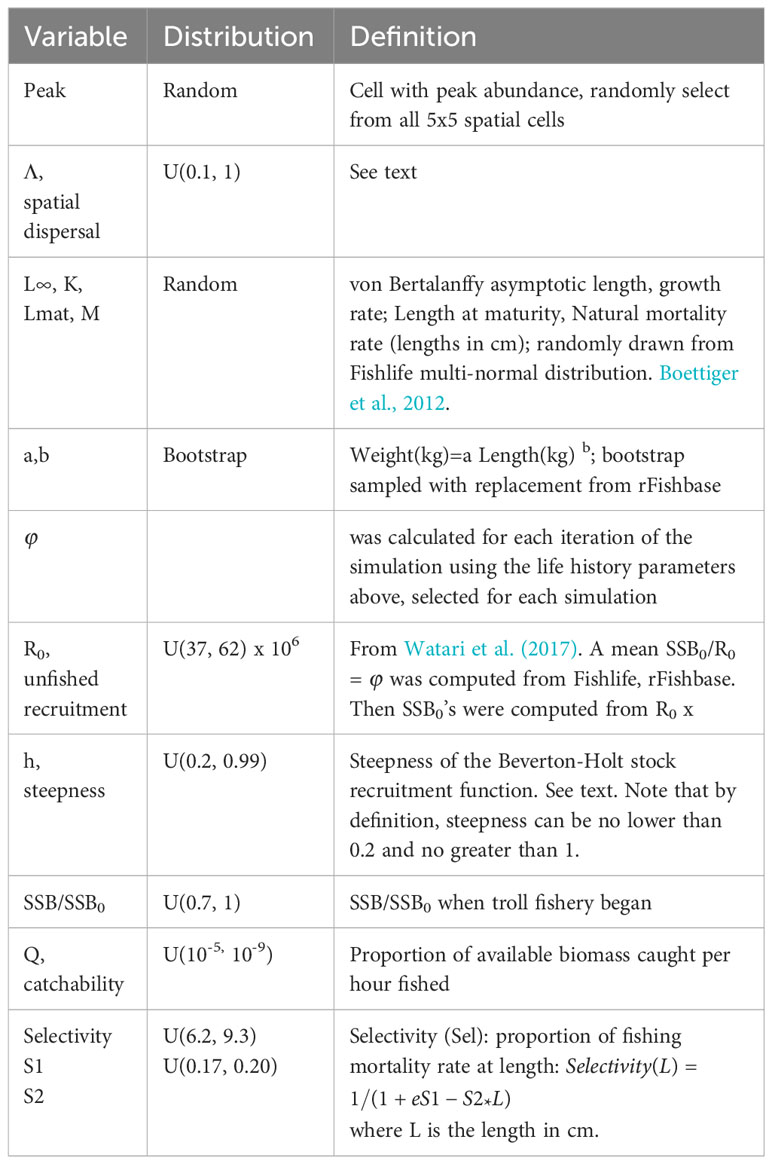
Table 3 Definitions of biological and population variables and their prior distributions used in the simulations.
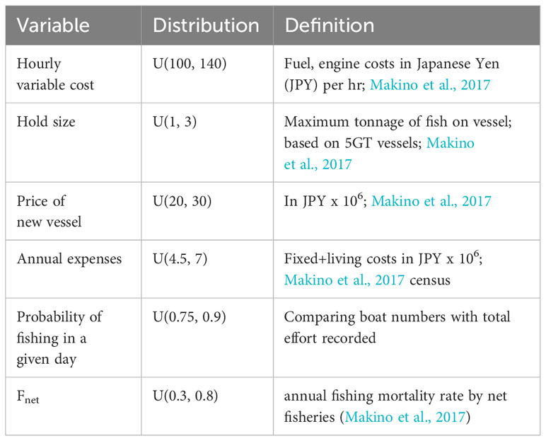
Table 4 Definitions of economic and fishery variables and their prior distributions used in the simulations.
While the parameters (Tables 3, 4) are the first step in conditioning the operating model of population and fishery dynamics, a set of six filters were imposed to further constrain the conditioning (Table 5). These filters largely functioned as determinates of the range of predicted conditions that are feasible (“current” relating to 2011 conditions from Watari et al. (2017). The filters address the history of catches, current troll landings, current SPR, current number of vessels, current proportion of total catch comprised by the troll fishery and the historical duration (years) of the troll fishery.
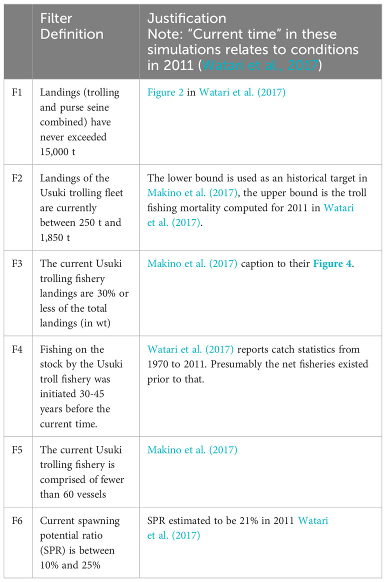
Table 5 Filters used to define the Usuki hairtail fishery operating model.
The rejection modeling phase models the time horizon from the initiation of the fishery.
Models were run from 2001 until 2011 where 2011 was the last year of data in the Watari analyses. The agent-based model with combined parameters was implemented using the six rejection filters. In total, the model was run for 354,775 iterations (approximately 24 hrs of computing time). and of these only 743 iterations satisfied all six of the filters. The extremely low acceptance rate (0.2%) demonstrates the effect of the wide priors in biological and fishery parameters. The original 354,775 iterations generated a suite of results where frequency distributions were based solely on the prior distributions (the solid lines and right-hand vertical axes in Figure 3). Then the results were screened by imposing first the F1 filter, then the F1 and F2 filter, F1, F2 and F3 filters and so on until all filters were imposed. At each of these steps the number of simulations which passed the filters decreases (the frequency histograms in Figure 3 using the left-hand vertical axes and the central tendency shifts.
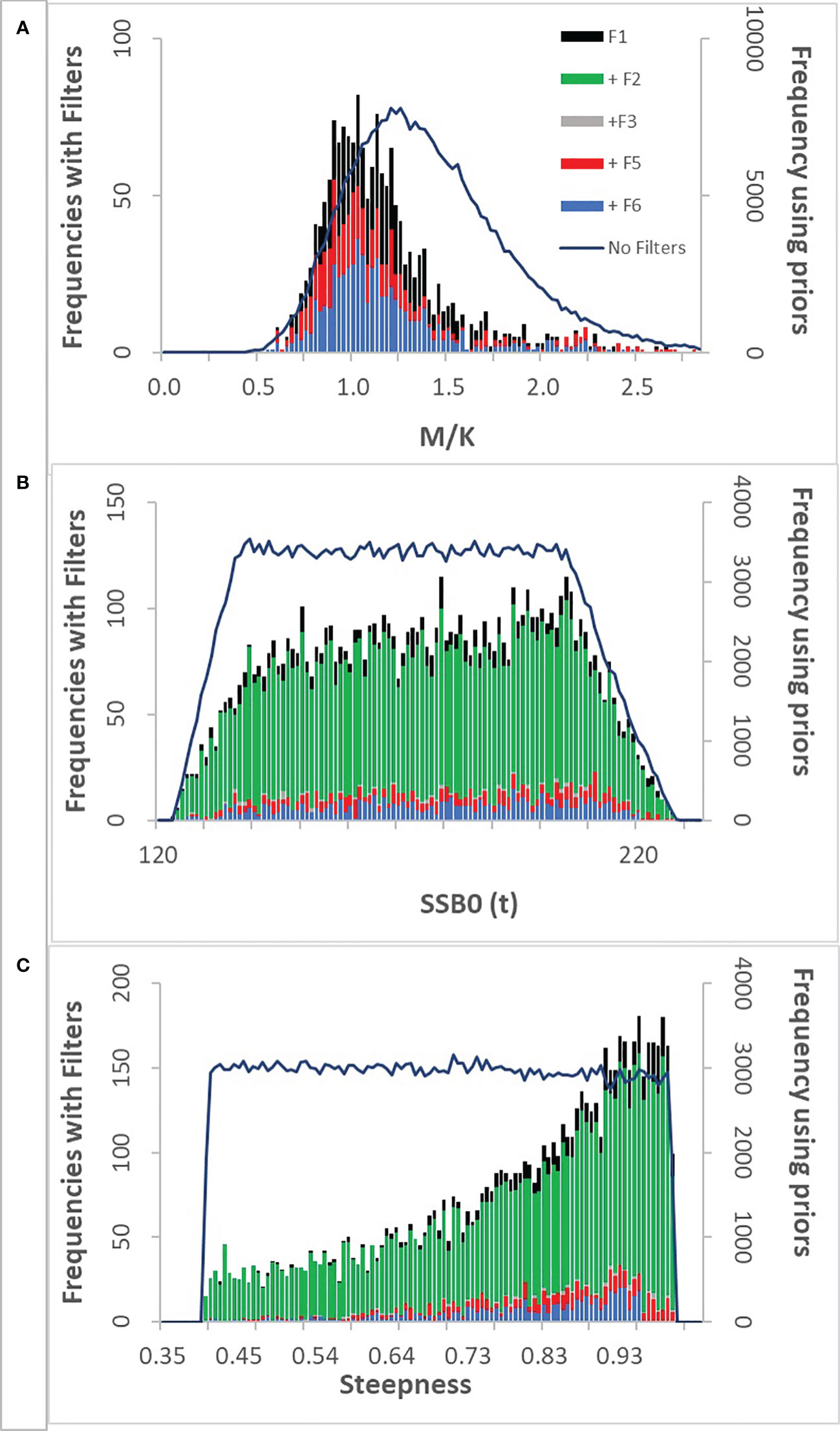
Figure 3 Frequency distributions of M/K(A), virgin spawning biomass (B) and steepness(C) from hairtail fishery simulations. The solid line is the frequency distribution of outcomes from the priors in Tables 3, 4 before being subjected to any of the filters (the prior frequencies are given in the right vertical axis). The left vertical axes are the histograms of frequencies of outcomes sequentially imposing the filters in Table 5: F1 means filter F1 passed, +F2 means F1 and F2 passed, etc. +F6 are the outcomes that passed all of the filters.
Adding additional filters does not materially change the frequency outcomes of virgin spawning biomass (SSB0). The distribution remains nearly uniform with the ends of the range being truncated (Figure 3). Steepness is also poorly determined but with frequencies accumulating at the higher end of the range (h > 0.7 more likely). The M/K distribution after application of the filters shows a modal value near 1 with a range of approximately 0.5 to 2 which is consistent with common “rules of thumb” for marine fishes (Beverton, 1992). Interestingly, the distribution of biomass in 2011 using just the priors exhibits a bimodal distribution (Figure 4A). Essentially, this results from the uniform priors generating a subset of parameters where biomass is on one side of the production curve (where the stock is not depleted) and another set on the depleted side. Then once the filters are added the biomass distribution reduces to unimodal and contracted to the lower end of the biomass range. The catch-related filters (F1, F2, F3) eliminate a large number of outliers and centralizes the distribution, but the current effort and SPR filters (F5 and F6) shift the mean biomass to higher levels. Note that the catch-related filters only address current conditions and not the history of catches. Additional filters relating to historical catch would be useful in defining fishery trends. Biomass in the stock assessment produced in Watari et al. (2017) is estimated at 4,896t in 2011. Here the mean biomass in 2011 after all filters were implemented was 3,477t with a standard deviation of 1,806t.
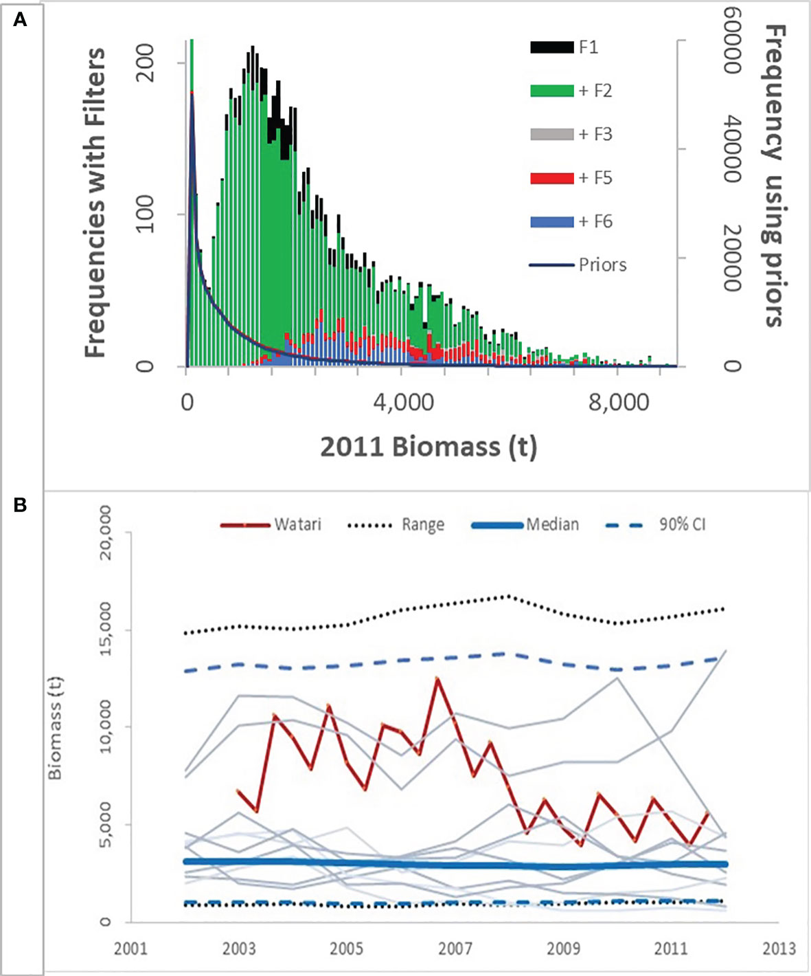
Figure 4 Frequency distributions of biomass in 2011 hairtail fishery simulations (A). The solid line is the frequency distribution of outcomes from the priors in Tables 3 and 4 before being subjected to any of the filters (the prior frequencies are given in the right vertical axis). The left vertical axis is the histogram of frequencies of outcomes sequentially imposing the filters in Table 5: F1 means filter F1 passed, +F2 means F1 and F2 passed, etc. +F6 are the outcomes that passed all of the filters. (B) the median, 90% CI and range of biomass trajectories compared to Watari et al., 2017. Additionally, the trajectories from 10 randomly selected simulations are plotted.
The biomass in Watari et al., 2017 (combining the two brood populations) was compared to the operating model from the rejection sampling (Figure 4). The operating model approaches Watari in the final year (2011), but exhibits more deviation in the preceding years. This is partially due to the filtering conditions (F2 to F5) focusing on current observations rather than trends but is primarily due to model misspecification. The Watari model estimated two large recruitment pulses in 2003 and 2005, and the biomass trends reflect this anomalous influx as it progressively entered and then disappears from the total biomass. The operating model was not conditioned on such large recruitment events and in fact does not allow such large yearly variations in recruitment.
Projections using the 743 operating model simulations (accepted by rejection sampling) were conducted in a simple management strategy evaluation. Three management strategies were evaluated and compared to the No Regulation case (no changes in fishing behavior from the operating model). The three strategies were: 1) No new entries, i.e. closed accessdisallowing new entrants or re-entry to the fishery and re-entry; 2) Seasonal closure, where fishing is limited to 200 days a year (combined with closed access), and 3) Increased selectivity, where a mandated gear modification is implemented changing hook and bait types that selects for larger fish as suggested by Hirose et al. (2017). This was modeled as a 10% increase in S1 and 10% decrease in S2 of the logistic selectivity (see Table 3). It was assumed these management strategies address the Usuki trolling fleet solely and that the fishing mortality by nets (primarily purse seines) are not affected.
Three performance metrics were evaluated that related to stock size and fishing effort. These were trajectories over a 15-year projection period of biomass, number of troll vessels in the fishery (a measure of effort) and Percent of Catch which relate to stock dynamics and fleet composition (Figure 5). The latter metric (Percent of Catch) is the percent of total catch (troll and purse seine) that is represented by the troll catch. Additionally, three economic metrics were evaluated (Figure 6). These were average annual savings per vessel, profits per vessel trip and revenue per hairtail catch (JPY/kg).
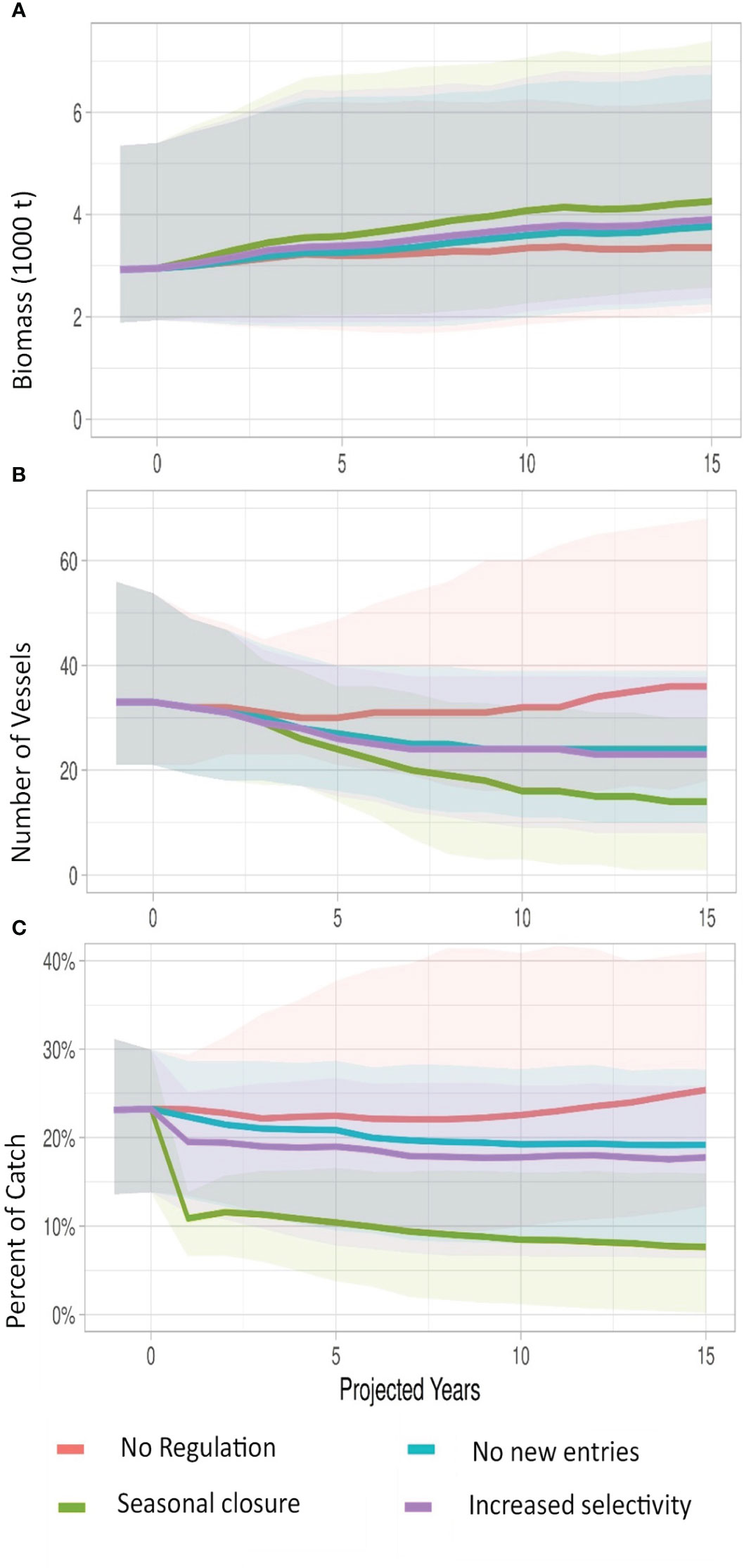
Figure 5 Median (bold) simulations of performance indicators under three policy options of 1) No new entries, i.e. closed access disallowing new entrants or re-entry to the fishery and re-entry; 2) Seasonal closure, where fishing is limited to 200 days a year (combined with closed access), and 3) Increased selectivity, where a mandated gear modification is implemented changing hook and bait types that selects for larger fish (see text). Indicators are: (A) hairtail biomass, (B) number active vessels and (C) percent of total landings comprised of troll catch. Shaded areas are 95% confidence intervals.
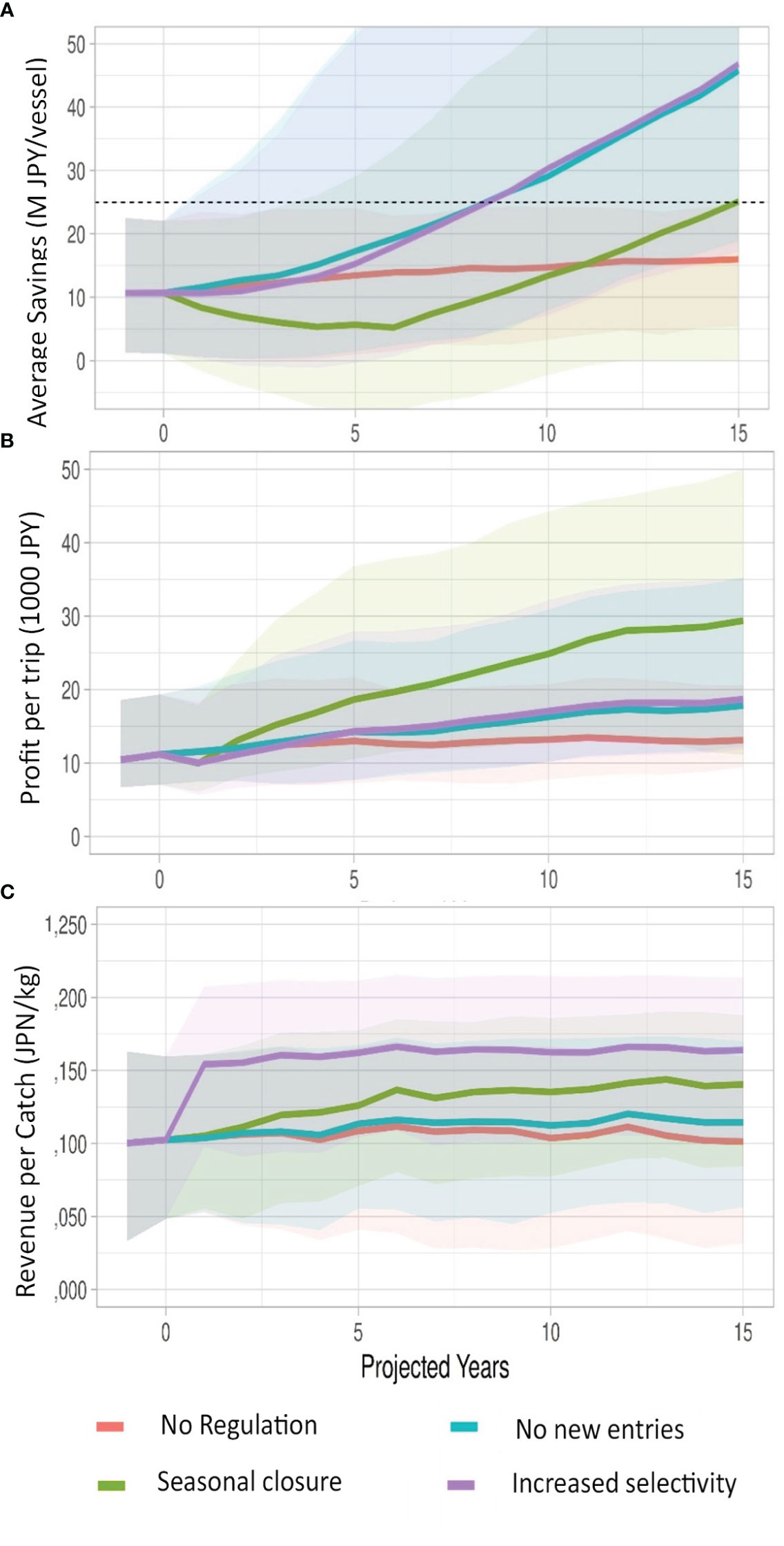
Figure 6 Median (bold) simulations of performance indicators under three policy options of 1) No new entries, i.e. closed access disallowing new entrants or re-entry to the fishery and re-entry; 2) Seasonal closure, where fishing is limited to 200 days a year (combined with closed access), and 3) Increased selectivity, where a mandated gear modification is implemented changing hook and bait types that selects for larger fish (see text). Indicators are: (A) average savings per vessel, (B) profit per vessel and (C) revenue per catch. Shaded areas are 95% confidence intervals.
Projecting a business-as-usual scenario with No Regulation shows a general stabilization over time (Figure 5) with little recovery in the median biomass. The landings are dominated by a stable net fishery in these projections with relatively small changes in the median number of troll vessels. Since the net catch is dominate and stable, the biomass does remains relatively stable but at a depletion level of 15%. All the three management strategies in one form or another are modifying fishing effort and reducing troll fishing effort. Thus, they all show a slow recovery of median biomass over the 15-year time horizon. Of these Seasonal closures perform best in terms of biomass recovery. However, this is achieved by decreases in vessel participation (Figure 5). Conversely, Increased selectivity performs well in terms of revenue per unit catch (Figure 6), as that strategy modifies the catch selectivity toward larger fish which achieves higher prices. Seasonal closures also, improves on this metric to a lesser degree. Seasonal closures also perform well in terms of profit per trip (Figure 6), as the reduced number of vessel trips capitalizes on the increased revenue per trip. However, these benefits are negated over time by the unmanaged purse seine fishery which increases its relative importance in landings as landings from the Usuki fleet decline. Further, while Seasonal closures generate higher profits per trip, these fail to cover fixed costs. A general feature of all these projections is the wide confidence intervals especially as projections extend beyond 4 or 5 years. Further exploration using subsets of the original parameter sets (i.e. alternative scenarios chosen from the rejection phase), would be important in defining robust strategies.
Also, there was a mismatch between the historical Watari et al. (2017) biomass and the median biomass from the rejection sampling (Figure 4). However, the current conditions (the conditions used for the start of the management strategy projections) were similar. In general, the historical mismatch would not detract from the projections as long as the starting conditions and production parameters were determined to be close to the real situation. The exception to this would be if a large recruitment deviation occurred shortly before the projection starting year and carried over into the projection phase. In that instance, the projections would also be mismatched. Therefore, the management strategy evaluation in this example (and for data-limited fisheries in general) is best viewed in a relative sense: does strategy “x” perform better than strategy “y”. One reason for this is the underlying lack of data to guide the conditioning phase (through the specification of filters). The reality of data-limited fisheries is the lack of a catch history. In this example, simple filters (F1, F2 and F3) only peripherally get at the catch history. And yet having a catch history is an important feature in stock assessments that help to define the scale of biomass of the stock.
The use of an agent-based approach in the context of a data-limited management strategy evaluation can be useful in that it builds in the dynamics of fishing effort directly into the evaluation through the underlying economic behavior model. This example demonstrates that the agent-based model can be conditioned with limited data. However, the actual computing time and the basic knowledge of the model required by users make it, perhaps, more difficult to implement than other approaches (Dowling et al., 2022; Carruthers et al., 2023).
The conditioning of any operating model relies on the integration of basic fishery statistics of catch, effort and abundance trends. In data-limited fisheries, methods have been developed to infer trends in these statistics for the fishery (Goethel et al., 2019; Dowling et al., 2022; Carruthers et al., 2023). This agent-based/rejection approach is an addition to these methods. In most cases the primary data-limitation is the lack of a history of fishery catches and effort. The agent-based approach essentially generates trends in effort based upon economic principles that are integrated with the model of stock dynamics. Then the rejection process filters the results to adhere to what is known about the fishery. In the hairtail example the filters on catch F1, F2 and F3 (Table 5) provide information on the scale, but implicitly the dynamics of the agent-based model provides information on trends in effort and, thus, fishing mortality. These effort dynamics are carried forward into the management strategy projections. Additionally, since MSE performance metrics often include effort (Goethel et al., 2019, i.e. vessels, participation), the agent-based approach explicitly models these quantities, as well as other economic indicators.
Rejection sampling is a procedure that lies within the continuum of methods to describe and bound uncertainty in stock assessments and operating models and to carry that uncertainty forward into MSEs. For example, using a parameter grid effectively is assuming that parameters in the grid are equally likely to have occurred (quasi-uniform fixed prior distributions); Monte Carlo simulations assume prior distributions of parameters are known and fixed; Bayesian approaches assume prior distributions of the parameters and then updates those distributions based on data. Rejection sampling assumes very vague parameter priors and implements those into an operating model through Monte Carlo methods, rejecting those model outcomes that are not feasible. Each of these methods is addressing uncertainty in the parameters and using that as guidance for determining an appropriate operating model for management projections and evaluations. All depend on the data and prior assumptions to generate those projections.
An important aspect of operating model conditioning and MSEs is to evaluate the effect of alternative scenarios (uncertainty in parameters and/or data) on current status and performance metrics. Essentially, this can be used to prioritize data collection (Goethel et al., 2019). In data-limited methods this is translated into testing alternative priors and their effect on results. In the hairtail case, the agent-based/rejection filtering provides an example. The distribution of current biomass (Figure 4A) shifts with the imposition of filters. The largest shifts occurred with the imposition of current effort and current SPR filters, indicating the importance of those data sources. Similar plots of performance metric distributions in response to filters can be made for selected times in the projections. Additionally, refined filters (alternative data scenarios) and the order in which the filters are imposed might be tested. An examination of the value of information to the determination of current conditions from the operating model and MSE projections can be useful. The effect of variations in parameter estimates on key status measures is especially useful with data-limited fisheries where parameter estimates have broad uncertainty. These types of analyses can assist in prioritizing data collection.
Rejection/agent-based methods of conditioning and MSEs can be used as an alternative to questionnaires, expert opinion (Dowling et al., 2022; Carruthers et al., 2023). However, ultimately all data-limited methods including rejection/agent-based are based on priors of individuals familiar with the fishery. The choice of methods will likely be made based on the practicalities of what is known about the fishery, the modeling expertise available and the suite of management strategies that are to be tested.
The original contributions presented in the study are included in the article/supplementary material. Further inquiries can be directed to the corresponding author.
Ethical review and approval was not required for the animal study because This study used published fisheries data; there was no contact with the animals. The studies were conducted in accordance with the local legislation and institutional requirements. Written informed consent was obtained from the owners for the participation of their animals in this study.
EC, conceptualization, methodology and writing, JP, visualization, technical review and writing, SS, RB, NP, KV-P, and JM contributed to analysis. All authors contributed to manuscript revision and approved the submitted version.
The author(s) declare financial support was received for the research, authorship, and/or publication of this article. This work was supported by the Oxford Strategic Partnership through a grant to support the development of the POSEIDON model for fisheries management.
We would like to thank current and previous funders of the POSEIDON project including: The Gordon and Betty Moore Foundation, The Walton family foundation, and Marine Stewardship Council.
The authors declare that the research was conducted in the absence of any commercial or financial relationships that could be construed as a potential conflict of interest.
All claims expressed in this article are solely those of the authors and do not necessarily represent those of their affiliated organizations, or those of the publisher, the editors and the reviewers. Any product that may be evaluated in this article, or claim that may be made by its manufacturer, is not guaranteed or endorsed by the publisher.
Bailey R. M., Carrella E., Axtell R., Burgess M. G., Cabral R. B., Drexler M., et al. (2018). A computational approach to managing coupled human–environmental systems: the POSEIDON model of ocean fisheries. Sustainability Sci. 14 (2), 259–275. doi: 10.1007/s11625-018-0579-9
Baker C. M., Gordon A., Bode M. (2017). Ensemble ecosystem modeling for predicting ecosystem response to predator reintroduction. Conserv. Biol. 31 (2), 376–384. doi: 10.1111/cobi.12798
Beaumont M. A., Cornuet J.-M., Marin J.-M., Robert C. (2009). Adaptive approximate Bayesian computation. Biometrika 96 (4), 983–990. doi: 10.1093/biomet/asp052
Beaumont M. A., Zhang W., Balding D. J. (2002). Approximate Bayesian computation in population genetics. Genetics 162 (4), 2025–2355. doi: 10.1093/genetics/162.4.2025
Beverton R. J. H. (1992). Patterns of reproductive strategy parameters in some marine teleost fishes. J. Fish Biol. 41, 137–160. doi: 10.1111/j.1095-8649.1992.tb03875.x
Boettiger C., Lang D. T., Wainwright P. C. (2012). Rfishbase: Exploring, manipulating and visualizing FishBase data from R. J. Fish Biol. 81 (6), 2030–2039. doi: 10.1111/j.1095-8649.2012.03464.x
Brooks E. N., Powers J., Cortes E. (2010). Analytic reference points fir age-structured models: Application to data-poor fisheries. ICES J. Mar. Sci. 67, 165–175. doi: 10.1093/icesjms/fsp225
Carrella E., Bailey R. M., Koed Madsen J. (2019). Repeated discrete choices in geographical agent-based models with an application to fisheries. Environ. Model. Software 111 (January), 204–230. doi: 10.1016/j.envsoft.2018.08.023
Carruthers T. R., Huynh Q., Hordyk A., Newman D., Smith A., Sainsbury K., et al. (2023). Method evaluation and risk assessment: A framework for evaluating management strategies for data-limited fisheries. Fish Fisheries 24, 279–296. doi: 10.1111/faf.12726
Carruthers T. R., Punt A. E., Walters C. J., MacCall A., McAllister M. K., Dick E. J., et al. (2014). Evaluating methods for setting catch limits in data-limited fisheries. Fisheries Res. 153 (May), 48–68. doi: 10.1016/j.fishres.2013.12.014
Dowling N., Wilson J., Cope J., Dougherty D., Lomonico S., Revenga C., et al. (2022). The FishPath approach for fisheries managers in a data- and capacity-limited world. Fish Fisheries 24, 212–230. doi: 10.1111/faf.12721
Froese R., Winker H., Coro G., Demirel N., Tsikliras A. C., Dimarchopoulou D., et al. (2019a). On the pile-up effect and priors for Linf and M/K: response to a comment by Hordyk et al. on ‘A new approach for estimating stock status from length frequency data’. ICES J. Mar. Sci. 76 (2), 461–465. doi: 10.1093/icesjms/fsy199
Froese R., Winker H., Coro G., Demirel N., Tsikliras A. C., Dimarchopoulou D., et al. (2019b). A new approach for estimating stock status from length frequency data. ICES J. Mar. Sci. 76 (1), 350–351. doi: 10.1093/icesjms/fsy139
Goethel D. R., Lucey S. M., Berger A. M., Gaichas S. K., Karp M. A., Lynch P. D., et al. (2019). Recent advances in management strategy evaluation: Introduction to the special issue “under pressure: Addressing fisheries challenges with management strategy evaluation”. Can. J. Fisheries Aquat. Sci. 76 (10), 1689–1696. doi: 10.1139/cjfas-2019-0084
Goudriaan J. (1986). “Boxcartrain methods for modelling of ageing, development, delays and dispersion,” in The Dynamics of Physiologically Structured Populations, 1st ed. Eds. Metz J. A. J., Dierkmann O. (Berlin: Springer), 453–473.
Gourieroux C., Monfort A., Renault E. (1993). Indirect inference. J. Appl. Econometrics 8, 85–118. doi: 10.2307/2285076
Grimm V., Revilla E., Berger U., Jeltsch F., Mooij W. M., Railsback S. F., et al. (2005). Pattern-oriented modeling of agent-based complex systems: Lessons from ecology. Science 310 (5750), 987–991. doi: 10.1126/science.1116681
Hartig F., Calabrese J. M., Reineking B., Wiegand T., Huth A. (2011). Statistical inference for stochastic simulation models - theory and application. Ecol. Lett. 14 (8), 816–827. doi: 10.1111/j.1461-0248.2011.01640.x
Hirose T., Sakurai M., Watari S., Ogawa M., Makino M. (2017). Conservation of small hairtail Trichiurus japonicas by using hooks with large artificial bait: Effect on the trolling line fishery. Fisheries Sci. 83 (6), 879–885. doi: 10.1007/s12562-017-1142-9
Hordyk A. R., Carruthers T. R. (2018). A quantitative evaluation of a qualitative risk assessment framework: Examining the assumptions and predictions of the Productivity Susceptibility Analysis (PSA). PloS One 13 (6), e0199298. doi: 10.1371/journal.pone.0198298
Hordyk A. R., Ono K., Sainsbury K., Loneragan N., Prince J. (2014). Some explorations of the life history ratios to describe length composition, spawning-per-recruit, and the spawning potential ratio. ICES J. Mar. Sci. 72, 204–216. doi: 10.1093/icesjms/fst235
Hordyk A. R., Prince J. D., Carruthers T. R., Walters C. J. (2019). Comment on "a new approach for estimating stock status from length frequency data" by Froese et al., (2018). ICES J. Mar. Sci. 76 (2), 457–460. doi: 10.1093/icesjms/fsy168
Lee J. S., Filatova T., Ligmann-Zielinska A., Hassani-Mahmooei B., Stonedahl F., Lorscheid I., et al. (2015). The complexities of agent-based modeling output analysis. J. Artif. Societies Soc. Simulation 18 (4), 4. doi: 10.18564/jasss.2897
Makino M., Watari S., Hirose T., Oda K., Hirota M., Takei A., et al. (2017). A transdisciplinary research of coastal fisheries co-management: the case of the hairtail Trichiurus japonicus trolling line fishery around the Bungo Channel, Japan. Fisheries Sci. 83 (6), 853–645. doi: 10.1007/s12562-017-1141-x
Martell S., Froese R. (2013). A simple method for estimating MSY from catch and resilience. Fish Fisheries 14 (4), 504–514. doi: 10.1111/j.1467-2979.2012.00485.x
Mildenberger T. K., Taylor M. H., Wolff M. (2017). TropFishR : an R package for fisheries analysis with length-frequency data. Edited by S. Price. Methods Ecol. Evol. 8 (11), 1520–1527. doi: 10.1111/2041-210X.12791
Miller S. K., Anganuzzi A., Butterworth D. S., Davies C. R., Donovan G. P., Nickson A., et al. (2019). Improving communication: the key to more effective MSE processes. Can. J. Fisheries Aquat. Sci. 76 (4), 643–656. doi: 10.1139/cjfas-2018-0134
Prince J., Hordyk A. (2018). What to do when you have almost nothing: a simple quantitative prescription for managing extremely data-poor fisheries. Fish Fisheries 20, 224–238. doi: 10.1111/faf.12335
Punt A. E., Butterworth D. S., de Moor C. L., De Oliveira J. A., Haddon M. (2016). Management strategy evaluation: best practices. Fish Fisheries 17 (2), 303–334. doi: 10.1111/faf.12104
Russell S., Norvig P. (2009). Artificial Intelligence: a modern approach. 3rd ed (Upper Saddle River, NJ, USA: Prentice Hall Press).
Seijo J. C., Defeo O., Salas S. (1998). Fisheries bioeconomics: theory, modelling and management. (Rome: FAO Fisheries Technical Paper). Available at: http://www.fao.org/3/W6914E/W6914E02.htm.
Szepesvari C., Lattimore T. (2019). Bandit algorithms (Cambridge UK: Cambridge University Press). doi: 10.5812/ircmj.17%284%292015.21233
Keywords: rejection-sampling, agent-based, data limited, management strategies, fishery management
Citation: Carrella E, Powers J, Saul S, Bailey RM, Payette N, Vert-pre KA, Ananthanarayanan A, Drexler M, Dorsett C and Madsen JK (2024) Rejection sampling and agent-based models for data limited fisheries. Front. Mar. Sci. 11:1243954. doi: 10.3389/fmars.2024.1243954
Received: 21 June 2023; Accepted: 03 January 2024;
Published: 19 January 2024.
Edited by:
Melissa Haltuch, National Oceanic and Atmospheric Administration, United StatesReviewed by:
Kristin N. Marshall, National Marine Fisheries Service (NOAA), United StatesCopyright © 2024 Carrella, Powers, Saul, Bailey, Payette, Vert-pre, Ananthanarayanan, Drexler, Dorsett and Madsen. This is an open-access article distributed under the terms of the Creative Commons Attribution License (CC BY). The use, distribution or reproduction in other forums is permitted, provided the original author(s) and the copyright owner(s) are credited and that the original publication in this journal is cited, in accordance with accepted academic practice. No use, distribution or reproduction is permitted which does not comply with these terms.
*Correspondence: Joseph Powers, ai5wb3dlcnMuZmlzaEBnbWFpbC5jb20=
Disclaimer: All claims expressed in this article are solely those of the authors and do not necessarily represent those of their affiliated organizations, or those of the publisher, the editors and the reviewers. Any product that may be evaluated in this article or claim that may be made by its manufacturer is not guaranteed or endorsed by the publisher.
Research integrity at Frontiers
Learn more about the work of our research integrity team to safeguard the quality of each article we publish.