Submesoscale variability in a mesoscale front captured by a glider mission in the Gulf of Finland, Baltic Sea

Modern research methods enable unfolding the structure of the water column with higher resolution than ever, revealing the importance of submesoscale. Submesoscale processes have intermediate space and time scales of <5 km and a few days in the Baltic Sea. A glider mission was conducted in the Gulf of Finland in May 2018. The appearance of a mesoscale front as a response to the persisting NE–E winds was observed. Within the front, smaller scale features at a lateral scale of a km were apparent. The tracer patterns indicated the presence of two adjacent motions – cold (warm) water penetrating upward (downward) on the lighter (denser) side of the front. We suggest they were traces of ageostrophic secondary circulation emerging while the loss of the upwelling-favorable forcing arrested the strengthening of the front. The analysis showed favorable conditions for the baroclinic and wind-driven instability. Such circulations could work to equalize the differences in cross-front direction, affecting the stratification and acting against the persistence of the mesoscale front. The spatial spectra of isopycnal tracer variance revealed the depth-dependence of the spectral slopes at the lateral scales of 1–10 km in the upper part of the water column. The differing of the slopes in the density layers associated with the mesoscale front indicates that frontal dynamics contribute to the energy cascade.

1 Introduction

The growth in the resolution capabilities of ocean observations has unfolded a rich structure on lateral scales of a kilometer (Karimova and Gade, 2016; Lips et al., 2016; Carpenter et al., 2020). This scale, referred to as submesoscale, forms by the interplay between atmospheric forcing and mesoscale motions. Turbulent motions associated with atmospheric forcing mix the surface layer in the vertical and mesoscale horizontal flows advect water masses introducing lateral variability (Ferrari and Boccaletti, 2004). Dynamically ocean’s submesoscale is defined with order one Rossby and balanced Richardson number expressed respectively as $Ro=\frac{\zeta }{f}$ and $R{i}_b=\frac{f^2{N}^2}{b_y^2}$, where ζ is vertical vorticity, f Coriolis frequency, N² vertical buoyancy gradient and b_y horizontal buoyancy gradient (Thomas et al., 2008). Therefore, by definition, submesoscale is active in regions of strong horizontal buoyancy gradients, strong vorticity, and weak vertical stratification. However, observations have shown that energetic submesoscale can be triggered throughout the ocean (Thompson et al., 2016; Yu et al., 2019b).

Comprehending the nature of submesoscale proposes a challenge as the dynamics is neither fully two- nor three-dimensional. Although being constrained by geostrophic and hydrostatic momentum balance to some extent, submesoscale flows can break this balance to show a forward energy cascade (McWilliams, 2016). Fronts are recognized as one of the primary sources of submesoscale motions (Thomas et al., 2013; Garcia-Jove et al., 2022). Fronts are known to be subject to frontogenesis (Lapeyre et al., 2006), frictional forces (Thomas and Ferrari, 2008), baroclinic instability (Boccaletti et al., 2007), and baroclinic submesoscale instability (Fox-Kemper et al., 2008; Thomas et al., 2013). Frontal submesoscale efficiently transfers energy to small-scale diapycnal mixing and dissipation through induced submesoscale flows, resulting in modified stratification. Therefore, the horizontal variations are closely related to the changes in the vertical structure.

Frontogensesis is a process that leads to the local intensification of the horizontal buoyancy gradient, requiring an acceleration of the along-front velocity to hold the geostrophic balance in the cross-front direction. An ageostrophic secondary circulation emerges to compensate for the acceleration. The overturning circulation is directed from the anticyclonic (light) to the cyclonic (dense) side of the front as the relative vorticity near the surface intensifies. Downwelling (upwelling) results from the conservation of potential vorticity that requires the horizontal flow to be convergent (divergent) on the dense (light) side of the front (Spall, 1995). We refer the reader to Figure 3 of Spall (1995). While the up- and downwelling rates are high (Yu et al., 2019a), returning of the water parcels to their original depth away from the fronts takes longer. Meanwhile, the external forcing has a chance to interact with the upper ocean, meaning that, in the real ocean, the horizontal buoyancy gradient is simultaneously subject to frictional forces, which can lead to modifications in the heat fluxes (Thomas, 2005). The wind generates Ekman currents that de- or restratify the water column, depending on the orientation between the wind and the baroclinic geostrophic flow along the front. Downfront (upfront) winds are aligned with (oriented against) the frontal jet, driving denser (lighter) fluid over lighter (denser) (Thomas and Ferrari, 2008). We refer the reader to Figure 1 of Thomas and Ferrari (2008).

Downfront winds reduce the potential vorticity in the Ekman layer but can additionally induce secondary circulations that extract potential vorticity from the pycnocline (Thomas, 2005). The mixed layer deepens as a result. When the potential vorticity turns negative, the flow becomes unstable (Hoskins, 1974) and symmetric instability can develop if the mixed layer is deeper than the Ekman layer (Thomas et al., 2013). Produced slantwise overturning cell at the base of the front (Taylor and Ferrari, 2009) pushes the system toward zero potential vorticity (Thomas et al., 2013). Thus, the stratification is modified by a combination of restratification by frontal circulation and surface forcing induced mixing of the density profile by convection. If the front persists while being marginally stable to symmetric instability, baroclinic instability can restratify the water column through the generation of secondary circulation by releasing potential energy (Boccaletti et al., 2007).

A large part of the insight into the submesoscale processes has been achieved thanks to numerical simulations (Boccaletti et al., 2007; Thomas et al., 2008; Mahadevan et al., 2010), while observations are challenging due to the processes’ ephemeral nature (Yu et al., 2019a). However, focusing on the regions where the environment favors the presence of submesoscale flows, recent glider observations have well demonstrated fine-scale water column structure. For instance, Pietri et al. (2013) sampled an upwelling system and discussed a driving mechanism that could explain observed submesoscale variability compatible with cross-frontal cells. Further, Pérez et al. (2022) analyzed submesoscale instabilities in a warm core ring and showed the core to be susceptible to gravitational instability and the periphery to symmetric instability under favorable downfront wind forcing. While in the ocean, the use of gliders is common, only a few studies have been conducted using gliders in the Baltic Sea (Karstensen et al., 2014; Meyer et al., 2018; Carpenter et al., 2020; Liblik et al., 2022). Observations by towed and autonomous devices (e.g., Lips et al., 2016; Carpenter et al., 2020) have indicated the presence of submesoscale activity, but the analysis of their nature is lacking.

Understanding the dynamics of the submesoscale allows for improving numerical models to which a physically complex environment like the Baltic Sea proposes a challenge (e.g., Tuomi et al., 2012). In the Baltic Sea, the water column has a layered structure that forms due to the atmospheric forcing and input of fresh river water and saltier North Sea water. Although, in general, the sea is shallow, the depth varying from a few tens of meters to a hundred meters determines the characteristic structure of the water column. The thermohaline structure can have one, two, or three layers. Halocline is persistent at 50–70 m in most of the deeper areas (e.g., Alenius et al., 2003; Liblik and Lips, 2017), and the seasonal thermocline usually develops above 20 m during spring (e.g., Alenius et al., 1998; Liblik and Lips, 2017). The presence of submesoscale flows and features has been often indicated together with rich mesoscale variability (Kikas and Lips, 2016; Zhurbas et al., 2019). Numerous upwelling and downwelling events, fronts, and eddies are characteristic features of the Baltic Sea (Pavelson et al., 1997; Myrberg and Andrejev, 2003; Lehmann et al., 2012). In this study, we use high-resolution glider observations that reveal multi-scale variability of the water column.

A glider mission was conducted in the Gulf of Finland during the formation of the seasonal thermocline. The hypothesis that energetic submesoscale occurs within the mesoscale lateral density gradient under certain atmospheric forcing was tested. The study provided evidence of the frontal submesoscale processes and enabled their preliminary characterization. To our knowledge, the present investigation is the first attempt to study submesoscale processes in a repeated coastal-offshore transect in the Baltic Sea. The paper is organized as follows: Section 2 introduces the observational data and used methods; Section 3 describes the wind forcing and the observed water column structure concerning both the mesoscale and the submesoscale ranges; Section 4 discusses the observed features and their relation with the wind and the stratification; the last section summarizes the work.

2 Data and methods

2.1 Glider observations

The geographic area and season suggest the potential presence of larger-scale horizontal buoyance gradients. Salinity increases from east to west due to the large river discharge at the eastern end of the gulf (Ylöstalo et al., 2016) and a cross-shore temperature gradient could form due to faster warming in shallow areas (Lips et al., 2014; Lips and Lips, 2017). Furthermore, pycnoclines have varying cross-shore inclination depending on the local wind forcing (Liblik and Lips, 2017).

The data set analyzed in the study was gathered from 9 May to 6 June 2018 using an autonomous underwater vehicle – the Slocum G2 Glider MIA deployed in the Gulf of Finland slope area at 59.57° N–25.05° E, Baltic Sea (Figure 1). The glider collected oceanographic data along the 18 km long transect (S–N direction, sampled 26 times). The Slocum glider can perform YOs without reaching the surface. The mission set-up determined the glider to perform 4 YOs between surfacings (i.e., a cycle). The vehicle started turnaround either 4 m before the surface or 6 m before the seafloor. The glider moved at a horizontal speed of 0.32 ± 0.09 m s^-1. The average distance between the profiles near the surface was 287 ± 39 m (it reduces with depth due to the sawtooth-shaped sampling trajectory), and a profile took 7.8 ± 0.5 min to complete at a characteristic depth of 80–90 m. Therefore, the glider completed a cycle approximately in an hour after covering about a km horizontally.

FIGURE 1

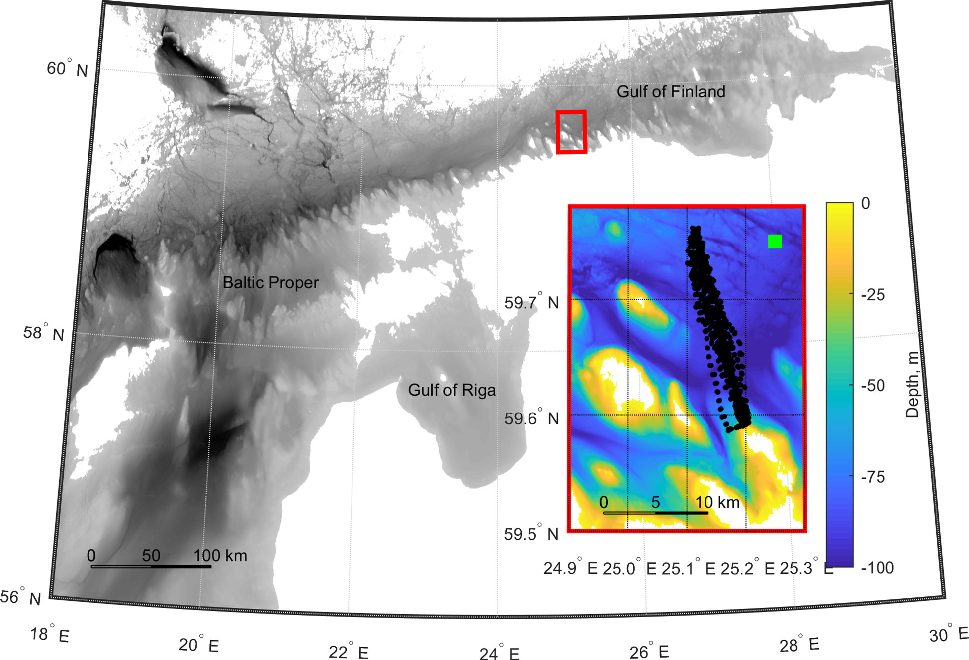
Figure 1 Map of the study area in May 2018. The overlaid plot shows the bathymetry (EMODnet digital terrain model) of the deployment area highlighted by a red rectangle. Black dots indicate the glider inflections on the surface. The green square shows the position of the ERA5 grid point used for the wind data.

Temperature and conductivity (salinity) profiles were collected with a pumped Seabird conductivity-temperature-depth recorder (CTD; model G-1451). Technical specifications of the sensors set the accuracy for pressure 0.1% of the full range (0–200 m), for temperature 0.002°C, and for conductivity 0.01 mS cm^-1. The CTD had a sampling rate of 0.5 Hz, and both descending and ascending profiles were recorded. Altogether over 4000 CTD profiles were gathered and analyzed. The raw data was quality controlled, and the coefficients to account for the response time of the sensors and the thermal lag were defined to minimize differences between two consecutive CTD profiles (Appendix). The typical vertical resolution of the raw CTD data was around 0.2 dbar. The half YOs were bin-averaged to a uniform 0.5 dbar vertical grid and arranged as profiles, meaning an average time and coordinates were attributed to a half YO. While the glider data has time-varying orientation in horizontal direction, for this analysis, each transect was interpolated on a regular grid with a latitudinal step of 0.0018° (if not specified otherwise). The horizontal step, equal to 200 m, was slightly larger than the distance between half YOs generally (median 135 ± 56 m) and thus, the interpolated fields were smoother. Note that this median distance between half YOs corresponds to the horizontal distance between the midpoints of the half YOs.

2.2 Velocity

Velocity calculations from the glider observations are limited. Absolute geostrophic velocity can be produced using the hydrographic data and the additional information from the depth-averaged current, which is estimated over a cycle based on dead reckoning and GPS fixes at the surface. The relative geostrophic velocity components were calculated using the dynamic method based on the geostrophic relationships

$$\begin{array}{c}{v}_g=-\frac{1}{f}\frac{\partial \varphi }{\partial x}\\ u_g=-\frac{1}{f}\frac{\partial \varphi }{\partial y}\end{array}$$

where the geopotential, ϕ, is proportional to dynamic height, D, as

$$\varphi =gD$$

Coriolis parameter is noted with f and gravitational acceleration with g. Therefore, the horizontal pressure gradient is presented through the geopotential slope of an isobaric surface. The relative geostrophic velocity is evaluated using a dynamic height anomaly relative to a reference pressure. The dynamic height that depends on the density of the seawater was determined from the measured temperature and salinity profiles according to McDougall and Barker (2011) (IOC et al., 2010).

The relative geostrophic velocity component was estimated from the glider CTD data at a lateral scale of 5 km. The choice of reference level (85 dbar) was based on the lowest variability (i.e., standard deviation) of density along isobars, interpreted as the effect of the baroclinic velocity field becoming negligible there. To involve shallower profiles in the geostrophic velocity estimations, the stepped no-motion level method described in Rubio et al. (2009) was used. While the 2D nature of the glider data allows us to estimate only the across-transect component of the geostrophic velocity, the depth-averaged velocity components were rotated to be compatible with cross- and along-transect components. On average, the transect was tilted 14° to the left from the S–N axis. As the glider orientation was relatively stable along the path, the approach of using an average tilt was adopted for simplicity.

2.3 Horizontal and vertical gradients

Buoyancy is expressed as $by=g(1-\frac{\rho }{{\rho }_0})$, where ρ₀ is reference density of 1003 kg m^-3. Along-transect buoyancy gradients, $b_y=\frac{\partial b}{\partial y}$, with a step of 5 km, were calculated to characterize the observed mesoscale frontal structure. Note that the notation y stands for the along-transect component and notation x for the across-transect component from here on. The stratification of the water column was characterized by the squared Brunt-Väisälä frequency (vertical buoyancy gradient) $N^2=-\frac{g}{\rho }\frac{\partial \rho }{\partial z}$, where ρ is density and $\frac{\partial \rho }{\partial z}$ its vertical gradient.

2.4 Smaller scale variability

The analysis of smaller scale variability focused on temperature variations on the isopycnal surfaces. At the same density surfaces, water properties act as passive tracers, and the effect of internal waves is assumed negligible (Rudnick and Cole, 2011). The smaller scale signal was defined as the deviations from the smoothed isopycnal temperature field (moving average of 4 km). The length scale was chosen based on the internal Rossby deformation radius, which is typically 2–4 km in the Gulf of Finland (Alenius et al., 2003). The deviations visualize the patterns created by the smaller scale motions, including the submesoscale range.

2.5 Submesoscale analysis

2.5.1 Submesoscale instabilities

Potential vorticity can be used to identify the potential for flow instabilities. Potential vorticity with the opposite sign of the Coriolis parameter indicates the unstable flow (Hoskins, 1974). Glider sampling capabilities limit the calculation of potential vorticity. Following Thompson et al. (2016), the potential vorticity can be expressed as

$$q=(f+\zeta )N^2-\frac{b_y^2}{f}$$

Vertical vorticity, ζ, is given here by the along-transect gradient of the across-transect velocity. Cross-transect velocities and along-transect density variations make the dominant contribution only if the glider transect is perpendicular to the front, highlighting the main assumption for this estimate of potential vorticity. The buoyancy gradients are underestimated in the glider measurements if the front is crossed at an angle different from the perpendicular orientation (Thompson et al., 2016). Therefore, the poor representation of the submesoscale instabilities because of the observational biases should be considered. In this study, neither the position of the front nor the crossing angle can be estimated.

The instability types are identified by the balanced Richardson angle

$${\varphi }_{R{i}_b}={\tan }^{-1}({-R{i}_b}^{-1})$$

One could expect −90°<ϕ_Rib<ϕ_c , where ${\varphi }_c={\text{tan}}^{-1}(-1-\frac{\zeta }{f})$ and 0<Ri_b<1 near strong horizontal buoyancy gradients, meaning the dominance of symmetric instability (Thomas et al., 2013). We refer the reader to Figure 1 of Thomas et al. (2013) for further relations of ϕ_Rib in case of different submesoscale instabilities. Symmetric instability is favored under destabilizing atmospheric forcing. However, the upper mixed layer needs to be deeper than the convective layer for overturning motions to dominate over convective mixing induced by surface forcing (Taylor and Ferrari, 2010).

Without knowing the angle between the wind vector and the geostrophic shear, the ratio of the convective layer depth, h, to the mixed layer depth, H, cannot be estimated. However, Obukhov length, L_o, can be used along with the convective layer to analyze the depth where symmetric instability can be expected. The wind stress dominates the turbulence between the surface and L_o, and the combination of the surface and wind-driven buoyancy fluxes from L_o to the convective layer depth (Taylor and Ferrari, 2010). Thus, L_o. implies the presence of the symmetric instability region if it is small compared to H. L_o is expressed as

$$L_o=\frac{U_{*}^3}{\kappa B}$$

where κ is the von Karman constant and U_* friction velocity found from wind stress, τ_w, and reference density as

$$U_{*}=\sqrt{\frac{{\tau }_w}{{\rho }_0}}$$

(Taylor and Ferrari, 2010). Net surface buoyancy flux, B, is expressed as

$$B=\frac{g\alpha Q_s}{{\rho }_0{C}_p}+g\beta (E-P)S_s$$

where C_p the specific heat of seawater, α and β are the thermal expansion and saline contraction coefficients evaluated respectively from the surface temperature and salinity, and S_s is the surface salinity (Buckingham et al., 2019). The net surface heat flux, Q_s, is the sum of the net short-wave and long-wave radiation, and the sensible and latent heat fluxes. The net freshwater flux comes from subtracting precipitation, P, from evaporation, E. Positive values correspond to stabilizing conditions.

The study period was characterized by the formation of seasonal thermal stratification, meaning the upper mixed layer developed near the surface. We defined it as the minimum depth where ρ_z≥ρ₁+0.25 kg m⁻³ was satisfied (ρ_z is the density at depth z and ρ₁ at 1 m). However, this shallow upper mixed layer does not characterize the water layer where the submesoscale circulations associated with the mesoscale front would rise if present. Thus, the upper boundary of the cold intermediate layer (CIL), defined as a water layer of <3°C, was used as H. The CIL boundaries were set as the average density at 3°C and the upper boundary corresponded to 4.4 kg m^-3. The depth of the upper mixed layer further helps to estimate the ratio of the convective layer depth to the mixed layer depth because stronger stratification acts to impede the vertical mixing.

2.5.2 Wind-driven and baroclinic instability

Baroclinic submesoscale instability affects potential vorticity by returning it to a neutrally stable state (q< 0 → q = 0), but horizontal buoyancy gradient may be subject to other physical processes that change the stratification and can also modify potential vorticity to be positive through the processes (Thompson et al., 2016). The relaxation of isopycnals back towards the horizontal occurs over a period of days, providing a reservoir of potential energy (Boccaletti et al., 2007) and potential for surface wind stress to induce overturning circulations through horizontal Ekman flows (Thomas and Ferrari, 2008). Downfront (upfront) winds have a destratifying (restratifying) effect. Secondary circulations generated through the release of potential energy by baroclinic instability act to restratify the water column. The possibility for the emergence of wind-driven and baroclinic instability can be estimated from the related buoyancy fluxes that can be expressed respectively as equivalent heat fluxes

$$Q_{Ek}=-\frac{b_y{\tau }_x}{f}\frac{C_p}{\alpha g}$$

$$Q_{BCI}=0.06\frac{b_y^2{H}^2}{f}\frac{C_p{\rho }_0}{\alpha g}$$

The parametrizations are published respectively by Thomas (2005) and Fox-Kemper et al. (2008) but adopted for the glider data by Thompson et al. (2016). Negative Q_Ek reduces the stratification and corresponds to downfront wind orientation. However, Q_BCI is always a positive quantity. Note that Q_BCI relies on the simulation-derived coefficient, which may not be optimal in other regions. Here, the surface values for b_y and α correspond to 3 m depth to exclude the possible contamination from waves and/or surface glider maneuverer. We acknowledge that as only the along-track glider data is used to calculate the equivalent heat fluxes, the angle at which the glider crosses the horizontal buoyancy gradient can bias the results. While Q_BCI is mainly underestimated, Q_Ek can be affected in both ways. Q_Ek is well underestimated if the horizontal buoyancy gradient is captured poorly and a large along-front component present in reality is missed, or well overestimated if the wind is interpreted to have a larger along-front component than it actually has (Thompson et al., 2016).

2.6 Wavenumber spectrum

The dominating contribution to the energy fluxes at the submesoscale range in the transfer of energy from large to dissipative scales has remained debatable. We calculated the power spectrum of isopycnal temperature in the wavenumber domain, composing the data as a function of cumulative distance. Isopycnal temperature fields on a regular grid were constructed due to irregular sampling in both space and time. First, the temperature profiles were averaged in density bins (step 0.1 kg m^-3), and then interpolated on a grid with a constant horizontal step of 150 m. Averaging in advance allowed us to reduce the effect of spatial and temporal smoothening due to interpolation, which tends to bias spectra towards steepening (e.g., Wortham and Wunsch, 2014). Before taking Fast Fourier Transform, the linear trend was removed and Hanning window applied. The smoothed power spectrum was obtained using 31 elementary frequency bands for averaging. The number of elementary frequency bands can be equalized with the degrees of freedom to find confidence limits (95%).

The wavenumber spectra of isopycnal temperature were calculated in the density range of 3.6–6.0 kg m^-3 with a step of 0.1 kg m^-3 (covered depths from 3–50 m). The spectral slopes were estimated between the spatial scales of 1–10 km. The resolved horizontal length scale was not separated because the short data series limit the resolution of the spectrum and the scales where the transition between distinct dynamics occurs are not known. The glider sampled the 18 km long section repeatedly and thus, the lower wavenumbers than the one corresponding to 10 km were disregarded. The submesoscale in the Baltic Sea can be expected to be active around 1–2 km. The spectrum at <1 km was not analyzed due to greater uncertainties at smaller scales (Nyquist frequency corresponds to the spatial scale of 0.3 km).

2.7 Surface forcing

Atmospheric forcing is presented through wind, net surface heat flux, and freshwater flux. Parameters defining heat exchange between the atmosphere and the sea surface were extracted on the product grid cells that covered the study area (59.50–59.75° N, 25.00–25.25° E) for May–June 2018 from European Centre for Medium-Range Weather Forecasts atmospheric reanalysis data set (ERA5 hourly data on single levels from 1979 to present, horizontal resolution of 0.25°×0.25°, Hersbach et al., 2020; Hersbach et al., 2022). Hourly u- and v-components of wind at 10 m height, mean surface net short-wave and long-wave radiation flux, mean surface latent and sensible heat flux, mean total precipitation rate, and mean evaporation rate were used.

The net freshwater flux is converted to an equivalent heat flux as also used by Giddy et al. (2021)

$$Q_f={\rho }_0{C}_p\frac{\beta }{\alpha }{S}_s(E-P)$$

Wind components taken from the nearest cell to the glider section (59.75° N, 25.25° E) were smoothed by a Gaussian low pass filter for 6 h. Wind stress is expressed as

$$\tau =c_d{\rho }_a\left|U_a\right|U_a$$

where c_d is the drag coefficient (1.2 · 10^-3; Large and Pond, 1981), ρ_a the air density (1.2 kg m^-3), and U_a stands for wind speed. The cumulative wind stress (in N m^-2 h) is the product of wind stress and its duration, demonstrating the impact of the wind during a longer period.

3 Results

3.1 Surface forcing

Winds and buoyancy fluxes drive mixing in the near-surface layers and affect the development of stratification. In general, wind speed during the study period was <4.5 m s^-1 (Figure 2). At the beginning of the glider mission, E winds prevailed, being relatively strong on 9–12 May and subsiding afterwards (to an average of 2.5 m s^-1). On 18–19 May, stronger northerly winds occurred for a short period, while the last third of May was characterized by alternating E and W winds. The W winds were stronger, on average, 5.4 ± 2.0 m s^-1 compared to E winds of 3.8 ± 0.9 m s^-1. The strong W–NW winds started to prevail on 1 June. The cumulative wind stress perpendicular to the glider transect (approximately positive towards E) picks up the three distinct periods during the mission – from the beginning until 19 May, wind forcing was to W, after that until 31 May, forcing varied between E and W, and from 1 June, it was to E (Figure 2).

FIGURE 2

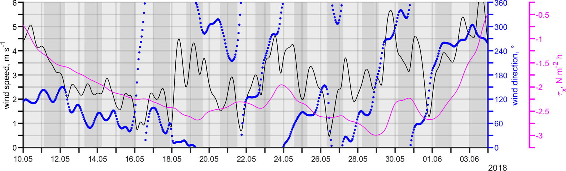
Figure 2 Wind forcing during the study period in May–June 2018 based on hourly data extracted from ERA5. Wind speed is shown in black and direction in blue, and cumulative wind stress in magenta. Shadowing indicates the orientation of the glider (light shows movement to N and dark to S).

3.2 Thermohaline structure

The mission was conducted during the formation of the seasonal thermocline. The distributions of temperature, salinity, density, and geostrophic velocity were constructed (Figure 3 shows the composite plots of the upper 25 m from the beginning, middle and end of the mission, 10 days apart). During the mission, the sea surface (0–4 m) temperature increased from 6.7 to 15.2°C, and the salinity decreased from 5.3 to 4.2 g kg^-1. The decrease in salinity indicates the advection of fresher water, which possibly originates from the eastern part of the gulf. The temperatures below the developing seasonal thermocline in the CIL were around 2°C, and the thermocline, characterized by the maximum temperature gradient of about 3°C dbar^-1, was observed at 10–15 m by the beginning of June.

FIGURE 3

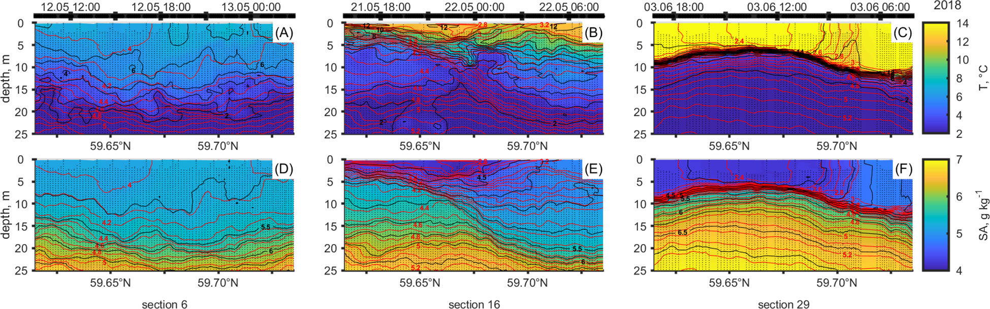
Figure 3 Temporal changes in temperature (A–C, black contours with a step of 1°C) and salinity (D–F, black contours with a step of 0.5 g kg^-1) distribution as a function of depth (0–25 m) along three glider sections in May–June 2018 (~10 days apart). The distributions are overlaid with red contours marking potential density anomaly with a step of 0.1 kg m^-3. The sampling timeline is at the top of the columns. The left side of a subplot is located closer to the coast and presents the southern part of the section. The area between ticks presenting latitude is about 2.7 km.

3.3 Horizontal buoyancy gradient

The mesoscale front was defined as an evident inclination in the density distribution, extending over the sampled transect. The horizontal (across-shore) buoyancy gradient formed as a response to the moderate NE–E winds that dominated for ten days prior to 19 May (Figure 2). The NE–E winds force surface waters to move offshore along the southern coast of the Gulf of Finland. Deep water rises in turn, tilting the pycnocline. Figure 4 shows the structure of the water column during the appearance of the front in the study window (~2.5-day period). The variability of buoyancy over the sampled section was small on 20–21 May, apart from the small area at the southern end of the transect, which indicated denser water rising (Figure 4A). However, a westward flow compatible with the geostrophic frontal jet appeared to be developing (Figure 4D). The frontal jet in thermal wind balance flows in the same direction as the wind. The buoyancy increased from south to north at 15 and 25 m depth on 21–23 May, indicating the presence of a horizontal buoyancy gradient (Figures 4B, C). The strong westward flow with velocities over 20 cm s^-1 spanning over the inclined density distribution suggested the presence of the frontal jet (Figures 4E, F).

FIGURE 4

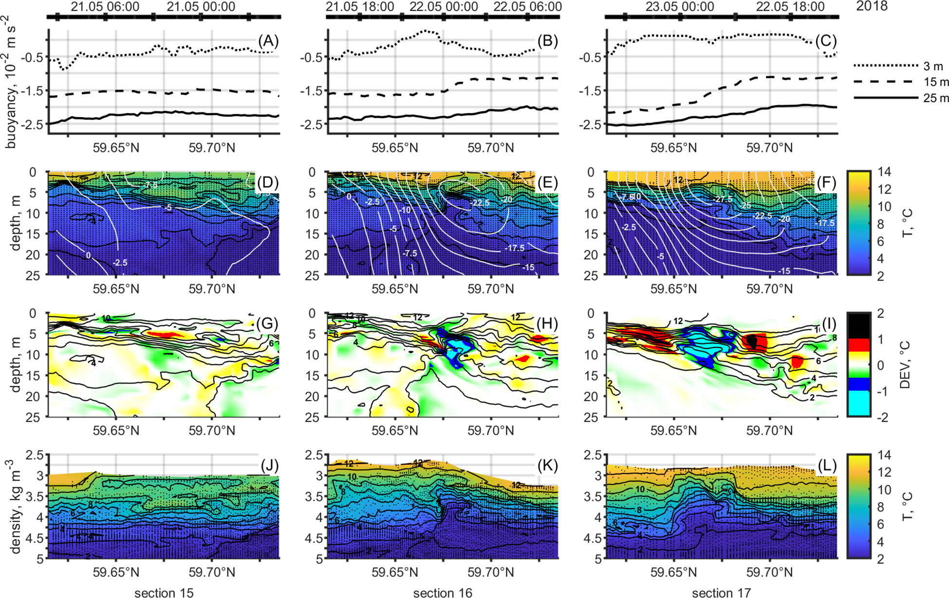
Figure 4 (A–C) Buoyancy along the glider transect at 3, 15, and 25 m depth on 20–23 May 2018. (D–F) Temperature distributions (black contours with a step of 1°C) as a function of depth (0–25 m) overlaid with white contours marking the relative geostrophic velocity (positive values show eastward movement) with a step of 2.5 cm s^-1 on 20–23 May 2018. The sampling timeline is at the top of the columns. The left side of a subplot is located closer to the coast and presents the southern part of the section. The area between ticks presenting latitude is about 2.7 km. (G–I) Temperature deviations as a function of pressure along the glider section on 20–23 May 2018. Black contours mark potential density anomaly with a step 0.1 kg m^-3. (J–L) Isopycnal temperature distributions (black contours with a step of 1°C) along the glider section on 20–23 May 2018.

The appearance of the front in the measurement window could be related to the stronger winds from N–NW on 19–20 May, meaning the generation of the front was not captured. The mesoscale front reaching the surface was not observed. Figure 5C shows smaller scale horizontal buoyancy gradients near the surface. They often had the opposite sign (a decrease of buoyancy from south to north) and were probably related to the fresher water advected into the study area. The mesoscale front persisted until June (Figure 5D), despite rather weak upwelling-favorable conditions alternating with the wind from the opposite direction in the last third of May. It is supported by the geostrophic velocities that exhibit persistence of the negative (westward) flow core. All measured temperature and salinity distributions with density distributions and geostrophic velocities are found in Supplement 1.

FIGURE 5

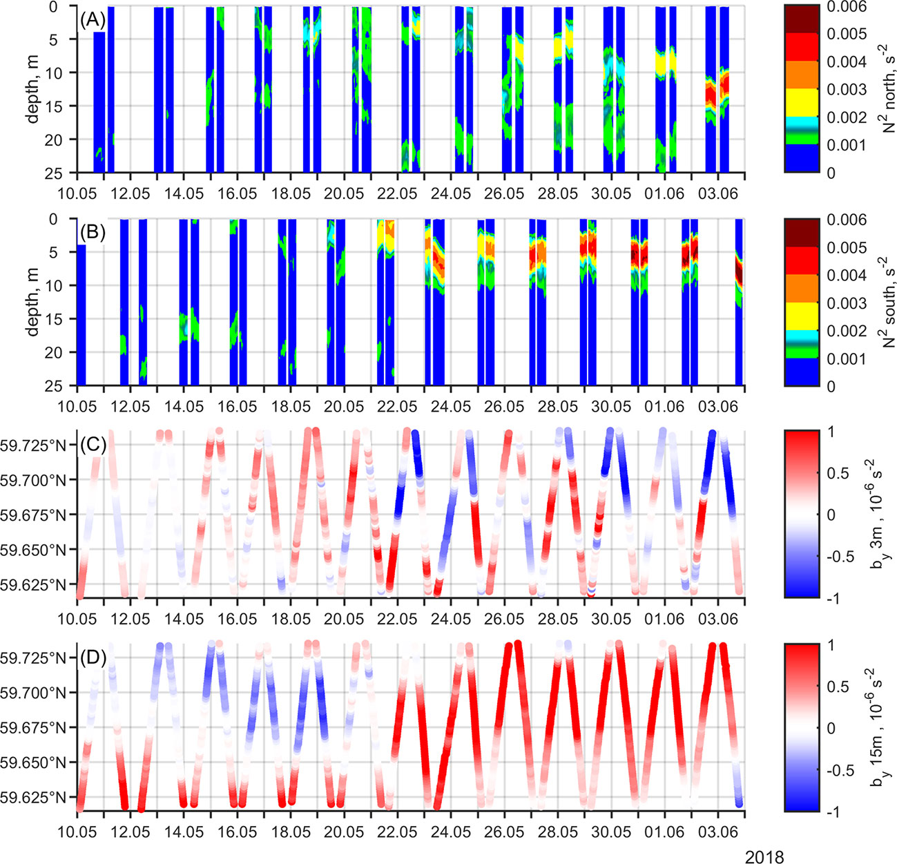
Figure 5 (A, B) Temporal changes in N² on the lighter and denser side of the mesoscale front in the upper 25 m, respectively. The lighter side is compatible with the position in the northern part of the glider transect (59.7242° N), and denser side with the position in the southern part (59.6252° N). Positions are 11 km apart. Note that one colored bar corresponds to about 1 km horizontal distance around the chosen position. To better illustrate the data, the distance correspondence in time is amplified about 5 times (bar width is increased). On average, the plotted distance was sampled in 1.4 ± 0.3 h. The movement of the glider between the southern and northern position can be deduced from subplots (B–D) that show along-transect horizontal buoyancy gradient as a function of time and latitude at 3, and 15 m depth, respectively. Positive gradient shows the increasing buoyancy along the sampled transect from S to N.

3.4 Vertical buoyancy gradient

Horizontal variations are closely related to the vertical structure. Figures 5A, B illustrates the change in the vertical stratification in the northern and southern part of the transect, compatible with the lighter and denser side of the front, respectively. The beginning of the mission was characterized by weak haline stratification (N² = 0.001 – 0.002 s^-2). The near-surface thermal stratification started to develop on 15–16 May. The appearance of the front on 21–22 May promoted the strengthening of the stratification on the denser side of the front because of the interaction between surface heating and vertical motions associated with the mesoscale front. The stratification was significantly stronger on the denser side of the front than on the lighter side, where actually two pycnoclines were observed after the appearance of the front.

The pycnoclines weakened and strengthened daily on both sides of the front. Pycnoclines on the lighter side appeared to be forced to merge episodically, indicating the alternating of the forcing and/or processes in favor and against the persistence of the front. We suggest that the weakening of the upwelling-favorable forcing arrested the strengthening of the front. Instead of collapsing abruptly, the front hosted ageostrophic frontal processes that equalized the differences in the cross-front direction by slowing the development of the stratification on one side of the front and promoting it on the other. The uniform stratification formed by 3 June over the course of a day, coinciding with the vanishing of the mesoscale front in the study area. Compared to the denser side of the front, the stratification remained slightly weaker on the lighter side.

3.5 Observed submesoscale pattern

To demonstrate the evolving smaller scale dynamics in the background of the mesoscale front, we analyzed the smaller scale thermohaline variability during the appearance of the horizontal buoyancy gradient. Isopycnal temperature distributions contrast water mass characteristics and/or visualize local diapycnal mixing spots. Figure 4K shows an intrusion manifested as a two-way intersection at 59.675° N – a cold water patch (around 3°C) penetrates through several isopycnal layers from 4.1 to 3.7 kg m^-3 and a warm water patch (around 8°C) penetrates from 3.3 to 3.7 kg m^-3. A similar pattern was observed at 59.65–59.675° N on the following day (Figure 4L), but not the day before (Figure 4J). Therefore, this structure emerged simultaneously with the appearance of the front in the measurement window.

Figures 4G–I demonstrates the smaller scale variations in the temperature by showing the deviations from the surrounding mean (4 km). Two adjacent temperature deviations with opposite signs characterizing the pattern indicated that the observed pattern consisted of two motions in opposite directions. Focusing on the described pattern, the deviations revealed extrema of 1.2°C and -1.4°C at 59.675° N on 21–22 May (Figure 4H). The extrema were larger on the following day (1.3°C and -2.1°C at 59.65–59.675° N, Figure 4I). The sign of the deviation indicated the water to originate from either shallower or deeper layers assuming that higher temperatures had their origin at the sea surface.

3.6 Submesoscale analysis

The last third of May was characterized by the persistence of the mesoscale front as well as the development of seasonal thermal stratification and the upper mixed layer, where the smaller scale horizontal buoyancy gradients formed. The diurnal cycle of net surface heat flux had a maximum of 400–500 W m^-2 (Figure 6A). The freshwater flux was insignificant compared to it. Previously described tracer patterns, which consisted of warmer water plunging down and colder water penetrating upward, were mapped repeatedly on the background of the mesoscale front. From here on, those intrusions are referred to as a submesoscale pattern.

FIGURE 6

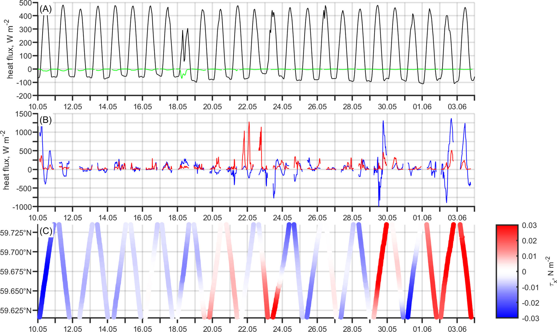
Figure 6 Equivalent heat fluxes associated with restratification processes during the study period in May–June 2018: (A) surface heat flux (black) and freshwater flux (green), (B) submesoscale overturning due to wind-driven processes (blue) and due to mixed layer baroclinic instability (red). (C) Component of wind stress perpendicular to the glider section as a function of time and latitude.

The structure of the submesoscale patterns suggests that they were traces of cross-front ageostrophic secondary circulation that is known to be generated while a horizontal buoyancy gradient is subject to baroclinic submesoscale, wind-driven and/or baroclinic instability. To identify whether the conditions favored the growth of different instabilities, the potential vorticity, and the equivalent heat fluxes related to restratification processes energized by surface wind forcing or the release of potential energy by baroclinic instability were calculated. Although the heat fluxes demonstrate the impact on the stratification, the elevated values also suggest the potential presence of frontal circulations.

The most pronounced submesoscale patterns captured during 21–23 May could be resulted from different physical processes. The period of the appearance of the mesoscale front in the study window coincides with the most significant episode of the equivalent heat flux related to baroclinic instability (Figure 6B), suggesting the pattern in Figure 4H to result from the frontal circulation generated through the release of potential energy by baroclinic instability. The equivalent heat flux related to wind-induced instability episodically also had comparable magnitudes (Figure 6B). However, this estimate is more likely to be more biased than the estimates suggesting baroclinic instability events. The negative equivalent heat flux from the surface wind forcing suggests destabilization of the water column and possible generation of the overturning circulation, extracting potential vorticity from the pycnocline. The water column structure captured on 23–24 May can be found in Supplement 1.

Downfront winds make the flow susceptible to symmetric instability by reducing potential vorticity. Figure 6C shows the component of wind stress perpendicular to the sampled transect, indicating downfront (upfront) orientation if positive (negative). The unstable flow is characterized by negative potential vorticity. Figure 7A demonstrates the dominance of positive potential vorticity that is in agreement with the development of the seasonal thermocline (relatively strong stratification) near the surface, but a stronger negative signal is found in the second half of the mission. Although the variety of instabilities can develop when q< 0, the ϕ_Rib criteria suggested the presence of only symmetric instability (i.e., 0< Ri_b< 1 and −90°<ϕ_Rib<ϕ_c ). The balanced Richardson number, which was always positive, showed the largest potential for symmetric instability in association with the mesoscale front on 23–24 May (elevated values at 5–10 m, Figures 7B, C). However, the Obukhov length was comparable with the depth of the upper mixed layer and the boundary of the CIL, meaning the criteria –H< z< -h was probably not satisfied. Although potential vorticity was reduced notably in the upper mixed layer in June, the relatively large Obukhov length suggested the convective layer depth to be similar in magnitude to the mixed layer depth, making the generation of symmetric instability still unlikely.

FIGURE 7

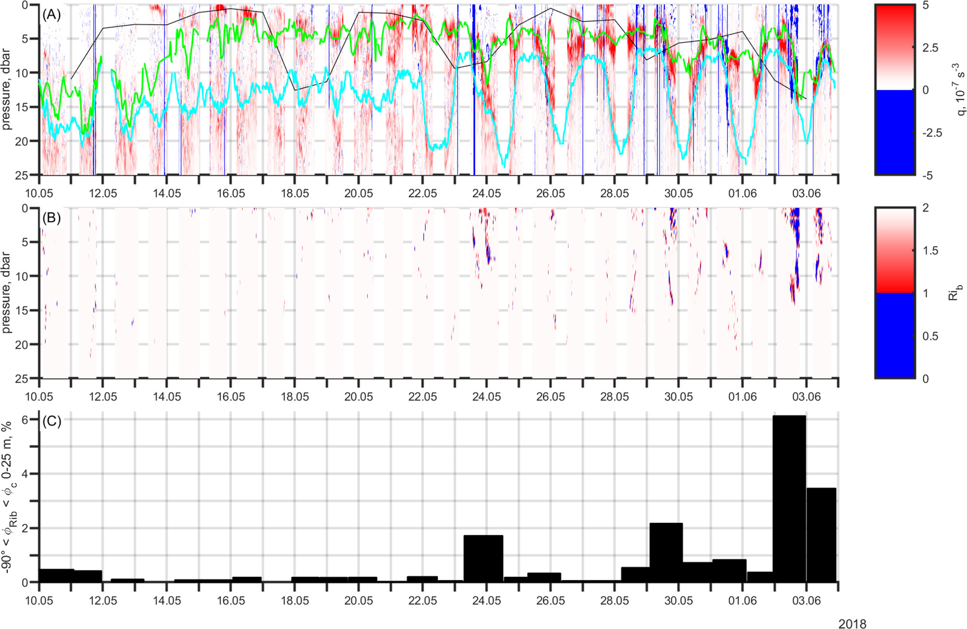
Figure 7 (A) Potential vorticity, q, and (B) balanced Richardson number, Ri_b, during the study period in May–June 2018. The Obukhov length (black), the depth of the upper mixed layer (green), and the boundary of the CIL (cyan) are shown with potential vorticity. We have emphasized respectively q< 0 and 0< Ri_b< 1 in solid blue. (C) The percentage of balanced Richardson angle in the range of –90° to determined critical angle of -45° in the upper 25 m per sampled transect.

The analysis suggests that the conditions favored the generation of the wind-induced and baroclinic instability, supporting the assumptions for the prevalence of the submesoscale despite the limitations: 1) the calculations relied on the assumption that the glider sampled perpendicular to the horizontal buoyancy gradient; 2) neither the position of the horizontal buoyancy gradients nor the angle at which the glider sampled is known; 3) poorly resolved individual submesoscale features, while sampling at an angle, can go unnoticed due to not satisfying the conditions of the analysis. Further conclusions should be made with caution as several assumptions were made (see section 2.5).

3.7 Wavenumber spectrum

Spatial variability of isopycnal temperature was analyzed in the upper part of the water column. The weakening of spectral energy on deeper isopycnals refers to the decrease in the temperature variability with depth (Figure 8). The slopes were estimated for the length scale from 1–10 km, and the individual σ-layers characterized by similar spectral slopes were averaged. The slopes for averaged spectra in the density ranges of 3.6–3.9 (3–10 m), 4.3–4.6 (10–20 m), 4.9–5.2 (15–25 m), and 5.7–6.0 (35–50 m) kg m^-3 were -2.14, -1.72, -1.84, -1.20, respectively. The slope was the gentlest on the isopycnals positioned in the CIL (5.7–6.0 kg m^-3). The slope near -1 suggests the applicability of the interior-quasigeostrophic theory and the domination of large-scale motions. Upper layers exhibit clearly steeper slopes, suggesting depth-dependence. The atmospheric forcing dominates in the uppermost layers, and energetic smaller scales stir the generated variability relatively efficiently. However, the trend of shallower spectral slopes with increasing depth did not express in the layers associated with the mesoscale front. This indicates the activity of frontal processes and their contribution to the energy flux.

FIGURE 8

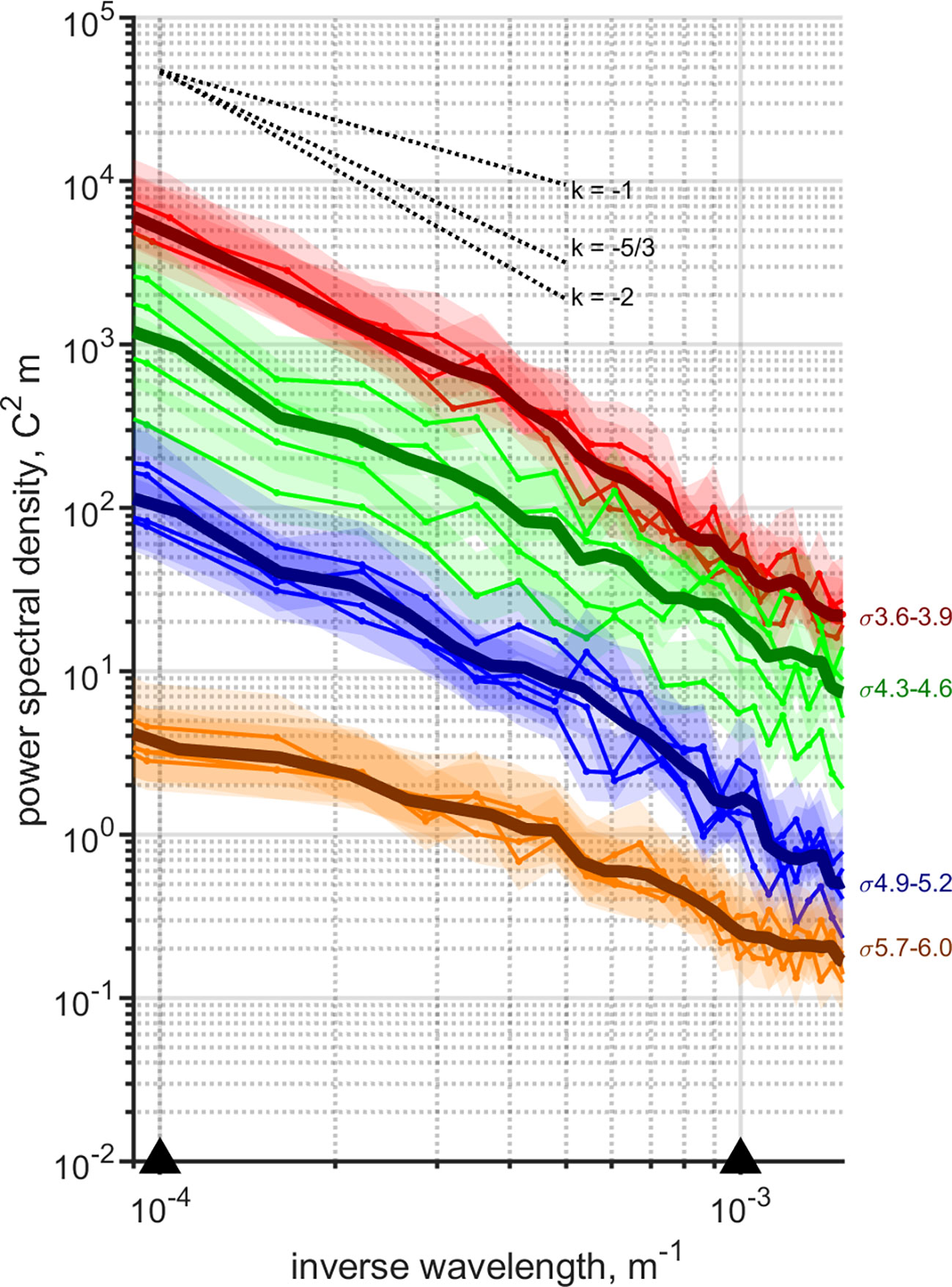
Figure 8 The wavenumber spectrum of isopycnal temperature of glider mission in May–June 2018. Thin lines present spectra along individual isopycnal surfaces (with a step of 0.1 kg m^-3) in the density ranges of 3.6–3.9 (red), 4.3–4.6 (green), 4.9–5.2 (blue), and 5.7–6.0 (orange) kg m^-3 with the shadowing showing the 95% confidence limits. Thick lines demonstrate the averages of the individual spectra. Black dotted lines show the slopes of -1, -5/3, and -2. From left to right, the black triangles are located at wavenumbers corresponding to 10 km and 1 km.

Constantly changing stratification affects the spectra but the extent of it is unknown. Additionally, rather short data series limit the spectral analysis. For that reason, the emphasis is more on the dynamics than the certain values of the slopes, which were near k^-2 in the upper part of the water column though. The observations support the suggestion that the submesoscale flows emerge within the mesoscale front revealed as the enhanced tracer variability in this layer compared to the variability in the layers above or below.

4 Discussion

Modern measuring vehicles such as gliders provide in situ data with sufficient spatial and temporal resolution to resolve the submesoscale successfully. The shallow depths in the Baltic Sea enable sampling at high resolution – profiles separated by 150 m on average are sampled under 10 min in the characteristic depth of about 100 m. Therefore, spatial scales of 1–10 km around the average Rossby radius (2–4 km; Alenius et al., 2003) are well resolved. In this study, we analyzed a month-long glider mission carried out in May–June 2018 and investigated the structure of the water column during the formation of the seasonal stratification. We elucidate the appearance of the mesoscale front in the study area, show the development of the stratification on both sides of the front, and characterize the associated elevated smaller scale variability. This data set provides a unique opportunity to resolve individual submesoscale features and analyze the potential mechanisms leading to their formation. We aim to demonstrate the occurrence of active submesoscale in the Baltic Sea under certain atmospheric forcing and hydrographic conditions.

4.1 Observed variability and possible drivers

The structure of the frontal submesoscale processes has remained theoretical despite the effort that has been devoted to observing the smaller scale variations. Although recent observational studies well support the presence of the frontal instabilities in the quiescent open-ocean environment, in the Subantarctic region, as well as near boundary currents (e.g., Callies et al., 2015; du Plessis et al., 2017; Yu et al., 2019b), few provide the information on the projection of submesoscale flows in the measurements (Pietri et al., 2013; de Verneil et al., 2019; Pérez et al., 2022). For instance, de Verneil et al. (2019) have demonstrated the orientation of fine-scale phytoplankton patches to be consistent with an ageostrophic secondary circulation generated by frontogenesis, providing, thus, the evidence on submesoscale flows modifying the vertical dynamics of phytoplankton.

According to the dynamical characterization, the coastal sea provides favorable conditions for the submesoscale processes. The transition to the open sea favors the colliding of water masses whether through the meeting of different flow structures or coastal processes like upwelling events, promoting, therefore, the formation of larger and smaller scale horizontal buoyancy gradients. By observing the coastal-offshore area at the end of spring 2018, we captured the appearance of the mesoscale front. The horizontal buoyancy gradient formed due to the wind-induced upwelling forced by the prevailing NE–E winds during the first ten days of the survey.

Simultaneously with the appearance of the mesoscale front, a pronounced submesoscale pattern emerged. The pattern showed upwelling of cold water on the lighter side of the front accompanied by downwelling of warm water on the denser side. The temperatures indicated the origin of the water from deeper or shallower layers, respectively, and, thus, suggested the presence of two adjacent movements in different directions. We suggest the presence of ageostrophic secondary circulation with a width of a couple of km on the profile of the mesoscale front between 5–10 m (Figure 3B). To support this suggestion, we attempt to infer the driving mechanisms that could explain the observed submesoscale activity.

A secondary circulation emerges in the form of an overturning cell as the front is subject to baroclinic, wind-induced, and/or baroclinic submesoscale instability. The submesoscale analysis revealed the large potential role of baroclinic instability on 21–22 May, suggesting that the observed submesoscale features resulted from the secondary circulations generated through the release of potential energy stored in the horizontal buoyancy gradient. The baroclinic instability can act together with surface frontogenesis (Lapeyre et al., 2006) but the surface signature was not observed in the study window. Additionally, the position of the captured feature on top of the mesoscale front is not compatible with frontogenetic secondary circulation that tends to subduct water below the front (Spall, 1995). Baroclinic instability occurs over a period of days (Boccaletti et al., 2007), indicating the possible interaction with the wind-induced instability. The analysis showed the effect of downfront winds that would counteract the restratification on the following days. On 22–23 May, the slope of the isopycnals was relaxed, and a few m deep upper mixed layer had formed (Figure 4F). Destabilizing atmospheric forcing can also favor symmetric instability. However, this is unlikely because the upper mixed layer needs to be deeper than the convective layer for overturning motions to dominate over convective mixing induced by surface forcing (Thomas et al., 2013).

The evolution of smaller scale variability in the background of the mesoscale front suggests the presence of several dynamical processes. Similar tracer patterns with various extent and intensity were mapped repeatedly until the end of the month, but the limitations of the glider observations complicate the interpretations. Fronts are a dynamical phenomenon and the 2D nature of the glider measurements prevents following the evolution of the front. In addition, observational biases should be considered when inferring the dynamical mechanism because of the adoptions for the glider data assuming the sampling perpendicular to the horizontal buoyancy gradient (Thompson et al., 2016). Further, the captured features are subject to soothing due to the effect of time-space aliasing.

4.2 Impact of wind

Horizontal variations are related to atmospheric forcing and to stirring by larger-scale flow fields. In the Baltic Sea, inclined pycnoclines and coastal upwelling events that appear as a response to winds are frequent (Lehmann et al., 2012; Liblik and Lips, 2017). The Gulf of Finland, a sub-basin of the Baltic Sea, is elongated in the W–E direction. The moderate winds blowing along the gulf are common (Keevallik and Soomere, 2014). The NE–E winds favor upwelling events near the southern coast of the gulf. A corresponding development of hydrographic fields was captured as a mesoscale front in the glider measurement window in May 2018. Although E and W winds alternated after 19 May, the mesoscale front persisted until early June.

The wind has a role in allowing the submesoscale flows to arise due to the disturbance of the balance when the external forces reduce and/or change. We have indicated that on 21–22 May, baroclinic instability appeared to develop during the temporary decrease in wind stress. Interpreting the orientation of the wind with respect to the geostrophic shear is challenging, but a rough estimate would be that the front was oriented approximately in the W–E direction at the sampling site. The sampled section positioned approximately along the S–N axis and the inclination in the density distribution that could be manifested as a front was observable. In accordance with this assumption, the wind changing from E to W direction indicates that mostly the wind had the component either up- or downfront. Thus, this variability of the wind would cause the alignment between the front and the wind direction to be lost or gained episodically (Mahadevan et al., 2010).

4.3 Impact on the stratification

The horizontal buoyancy gradients affect the stratification directly through the submesoscale processes. While the stratification is generated and destroyed through diabatic processes and frictional forces, frontal submesoscale can convert gradients from horizontal to vertical (McWilliams, 2016). Lateral variability introduced by the advection of water masses favors the appearance of horizontal buoyancy gradients and, in turn, suggests the emergence of the submesoscale. The glider observations revealed the complex structure of the water column. Atmospheric forcing acting on the sea surface contributed to the formation of the upper mixed layer and seasonal thermal stratification. The appearance of the mesoscale front created favorable conditions for the stratification to strengthen more rapidly in the southern part of the sampled transect as the mesoscale dynamics raised the isopycnals near the surface. We observed the stratification changing daily and developing differently on the denser and lighter side of the front (compatible with the southern and the northern part of sampled transect, respectively; Figures 5A, B). While the denser side was characterized by the strong stratification near the surface, two pycnoclines were observed on the lighter side.

We propose that the mesoscale front hosted ageostrophic frontal processes as the upwelling-favorable forcing weakened. The submesoscale circulations equalized the differences in the cross-front direction by slowing the development of the stratification on one side of the front and promoting it on the other. The overturning circulation induced by baroclinic instability slides dense water under light, acting to slump the front from the horizontal to vertical (Boccaletti et al., 2007). Thus, the baroclinic instability acted toward restratification on 21–22 May. The wind increased on the following days, suggesting the possible interaction with wind-induced instability. The overturning circulations acting toward restratification appeared to be dominating but the temporary return of the NE–E winds supported the persistence of the front. Two pycnoclines were observed on the lighter side of the front again on 27 May. However, the front appeared to shift toward the open sea (northern part), suggesting that partly the frontal circulations managed to restratify the water column. The presence of the submesoscale flows within the horizontal buoyancy gradient could have contributed to the development of the seasonal stratification. The effect of the submesoscale can be especially important during seasonal warming because stratification events can occur more rapidly than solely surface heating could drive (du Plessis et al., 2019). Enhanced stratification favors primary production (Swart et al., 2015).

4.4 Spectral analysis

While measuring submesoscale flow fields is challenging, the underlying dynamics can be deduced by investigating the variability of tracer fields along the same density surfaces (Callies and Ferrari, 2013; Jaeger et al., 2020). Submesoscale flows can cause substantial heterogeneity in tracer distribution because of their dynamics, which by its nature should connect fully two- and three-dimensional motions (McWilliams, 2016). Submesoscale processes have gained more attention in the Baltic Sea only in recent years, though (Lips et al., 2016; Carpenter et al., 2020). Lips et al. (2016) have presented the spectrum of an active tracer in the sub-surface layers (note that the tracer variance along the isobaric surfaces was evaluated). The spectra showed slopes closing to -2 at 1–10 km during periods of high variability of temperature due to upwellings. The discrepancy from -3 that is predicted by quasigeostrophic theory (Charney, 1971) was interpreted as the contribution of the ageostrophic submesoscale processes to the energy cascade.

The studies from the ocean environment are well presented (e.g., Cole and Rudnick, 2012; Callies and Ferrari, 2013; Kunze et al., 2015; Jaeger et al., 2020). However, the processes setting the spectra have remained obscure. In the open ocean, the -2 slope independent of depth has been reported at the submesoscale range (Cole and Rudnick, 2012; Callies and Ferrari, 2013). The main contribution to the energy at the submesoscale comes possibly from unbalanced flows. The characteristics of the Baltic Sea (e.g., the shallow depth, strong stratification, seasonality, negligible tidal forcing) distinguish the sea from the ocean, forming a dynamically complex environment (Tuomi et al., 2012). There are some studies carried out in the stratified environment. Kunze et al. (2015) found tracer variance spectra sloping with a k^-2 at the horizontal length scale 0.03–10 km in the seasonal pycnocline at 20–60 m depth. Evident fronts were not observed at every study site, though. On the other hand, Jaeger et al. (2020) showed steep slopes (k^-3) at 1–10 km in the stratified upper 75 m. Above 10 km scales the spectral slope was closer to -2. They proposed that ageostrophic dynamics could cascade variance in the pycnocline more rapidly than predicted. We, however, found gentler spectral fall-off in the layers associated with the mesoscale front compared to the layers above. This indicates that frontal submesoscale preserves tracer variability longer than the turbulence in the upper layers. The short data series acts as both an advantage and a disadvantage in this study while allowing us to analyze one specific situation but prevents broader conclusions. We will test this suggestion in a future study by incorporating a wide range of glider data sets from different seasons.

Observational spectra are independent of predictions and, thus, extensive data collections contribute to shaping understanding of the energy cascade. The observations have revealed the discrepancies from the quasigeostrophy, but often the limitations prevent identifying the reasons. We conclude that the contribution of the ageostrophic frontal effects is likely in the upper part of the water column (0–25 m in the Baltic Sea). The depth-dependence may be related to the stratified environment as it was noticed here and by Jaeger et al. (2020). Flatter spectral slopes in the deeper part of the water column coincide with stirring by two-dimensional homogeneous turbulence that leads to a tracer spectrum following k^–1 (Callies and Ferrari, 2013).

5 Conclusions

Mostly the presence of submesoscale phenomena in the Baltic Sea has been demonstrated using numerical modeling (e.g., Väli et al., 2017), and observational studies are scarce. This is the first study analyzing individual submesoscale features in a coastal-offshore transect of the Baltic Sea. The glider measurements gathered at the end of spring 2018 revealed smaller scale features within the mesoscale front. Submesoscale tracer patterns, characterized by two adjacent motions showing the upwelling on the lighter and downwelling on the denser side of the front, were captured. We proposed they were traces of the frontal submesoscale circulations, as the analysis suggested favorable conditions for the baroclinic and wind-induced instability. The frontal submesoscale acted against the persistence of the front. The constant presence of submesoscale variability in the background of the front indicates active submesoscale flows in the Baltic Sea. In addition, the role of the submesoscale processes appeared to increase under reduced wind stress. This result emphasizes the need for further studies, as the classical expectation is that strong vertical mixing occurs through turbulence when wind speeds are high.

6 Appendix

Minimizing instrumental error is important when the analysis focuses on the small-scale variability. Gliders are known to provide high spatial resolution in the vertical but only in one horizontal direction. Small errors in profile-to-profile measurements modify the data artificially. In this study, all applied corrections rely exclusively on the glider data and assume that compared consecutive profiles correspond to the same water mass. Consecutive profiles refer to the profiles that are the closest to each other in space (the parts of profiles with a "∧" or "∨" shape, Figure 9E) because the largest errors associate with the strong gradients. The Baltic Sea is strongly stratified – the upper (lower) pycnocline coincides with the thermocline (halocline).

FIGURE 9

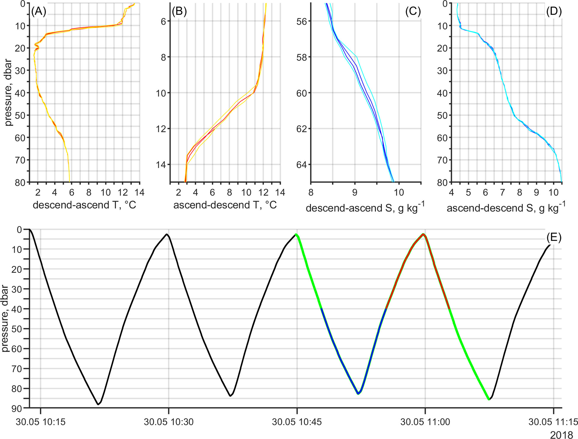
Figure 9 (A, B) Examples of raw (yellow) and corrected (response time, red) temperature profiles respectively over the water column and the thermocline depth range in case of descend-ascend (highlighted with blue in E) and ascend-descend (highlighted with red in E). (C, D) Examples of raw (cyan) and corrected (thermal lag, blue) salinity profiles respectively over the halocline depth range and the water column in case of descend-ascend and ascend-descend. (E) An example of a cycle shown as a time series of pressure. Green highlights the consecutive profiles. Overlaid blue shows the parts of profiles with a "∨" shape, and red a "∧" shape.

First, temperature and conductivity sensors are subject to response time. While transiting through strong vertical gradients, the water properties can change quicker than the sensor is capable of registering, resulting in the misalignment of the measurement with pressure. The lag is in opposite direction for a descend and an ascend because of the transition direction, for example first from warmer to colder (fresher to saltier) water and then reversely. Next, the conductivity cell’s capacity of storing heat causes small errors in inferred salinity. The effect is referred to as thermal lag. Measured temperature corresponds to the ambient temperature of the conductivity cell, but conductivity is measured inside the cell. To obtain accurate salinity estimate, measured temperature is reassessed. The temperature inside the conductivity cell is evaluated by subtracting the correction, T_tl, from the temperature readings, T. The correction is found using the relation:

$$T_{tl}(n)=-b{T}_{tl}(n-1)+a[T(n)-T(n-1)]$$

Coefficients a and b are determined by

$$a=\frac{4f_n{\alpha }_{tl}{\tau }_{tl}}{1+4f_n{\tau }_{tl}}$$

$$b=1-\frac{2a}{{\alpha }_{tl}}$$

where f_n is the sampling frequency, α_tl amplitude of the temperature error, and τ_tl relaxation time constant (Mensah et al., 2009).

A linear time shift was applied to temperature and conductivity according to the estimated data misalignment with pressure. A similar method with varying shifts has been presented by Bishop (2008), and Garau et al. (2010) have shown the concept of minimizing the area between two profiles. The time shifts were varied from 0 s to 3 s by 0.1 s steps. The mean area (trapezoidal method) were calculated between two consecutive profiles at the depth range of 20 m around the depth of the strongest gradient. The median of the area was found for each time shift and the optimal time shift was chosen based on the lowest one under the assumption of lowest discrepancy between profiles. In this study, the temperature was re-aligned by 1.4 s and conductivity by 1.1 s (Figures 10A, B).

FIGURE 10

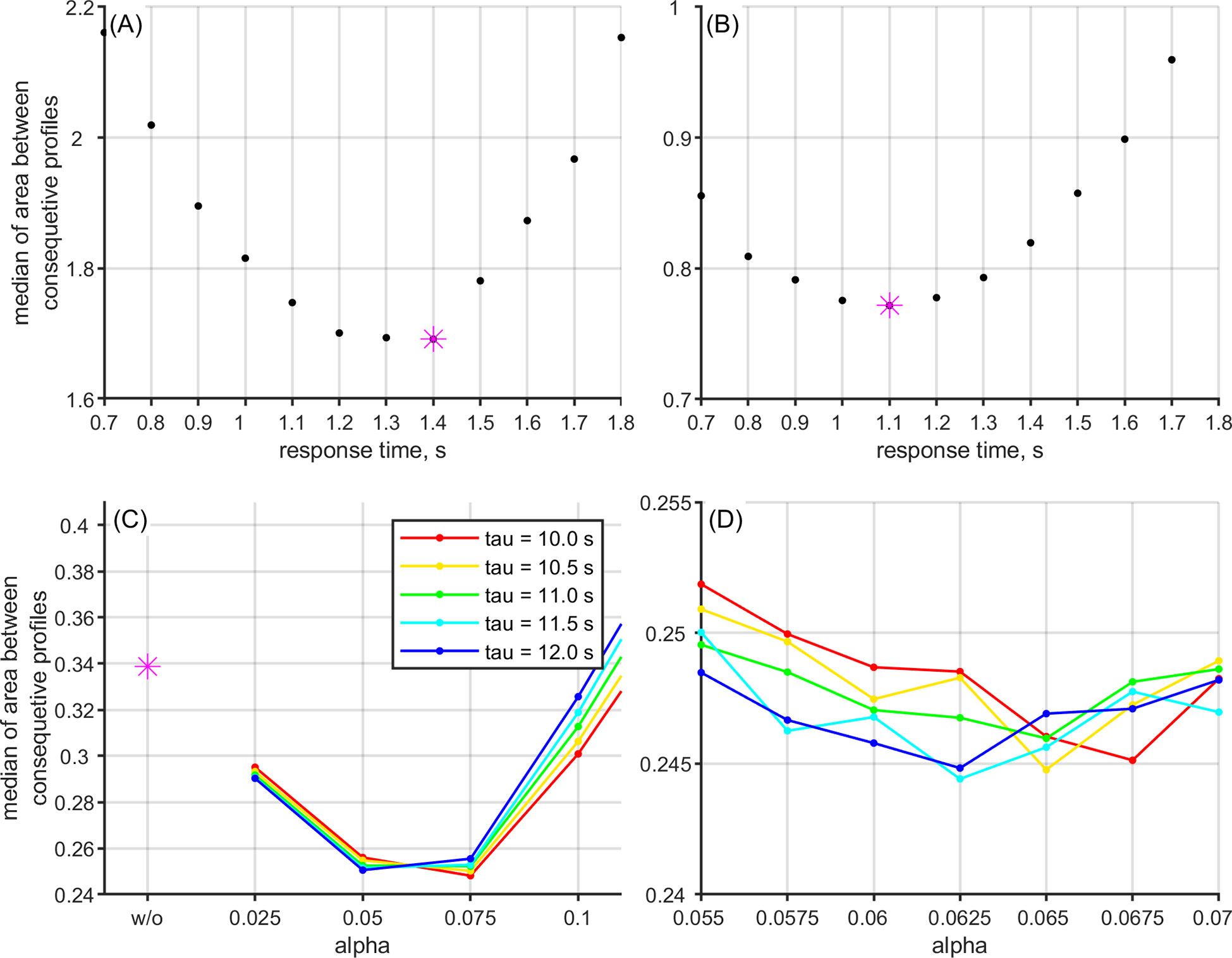
Figure 10 (A, B) The change in the median of the mean area between profiles as response time correction was applied respectively for temperature and conductivity. The optimal time shift is shown with magenta star. (C, D) The change in the median of the mean area between profiles as thermal lag correction was applied with respect to the one calculated based on the raw data (magenta). The median value decreases at first as α_tl increases. Colored lines correspond to τ_tl values from 10 to 12 s with 0.5 s step. The optimal combination of α_tl and τ_tl were chosen near minimal median value (D).

We show the quality of the correction based on temperature. Figures 9A, B shows the examples of corrected temperature profile. Full profile is shown for the case descend-ascend (shape "∨"), and the depth range of the upper pycnocline for the case ascend-descend (shape "∧") to better demonstrate the agreement between the corrected profiles. Figures 11A, B shows the discrepancy between two consecutive profiles shown in Figures 9A, B. The profiles show better agreement in case of ascend-descend because the data in the thermocline range is measured with little time separation. Figures 11E, F shows the histogram of discrepancies for all the compared profiles. The skew present in the discrepancies between raw profiles is removed after shifting despite comparing descend with ascend or the opposite.

FIGURE 11

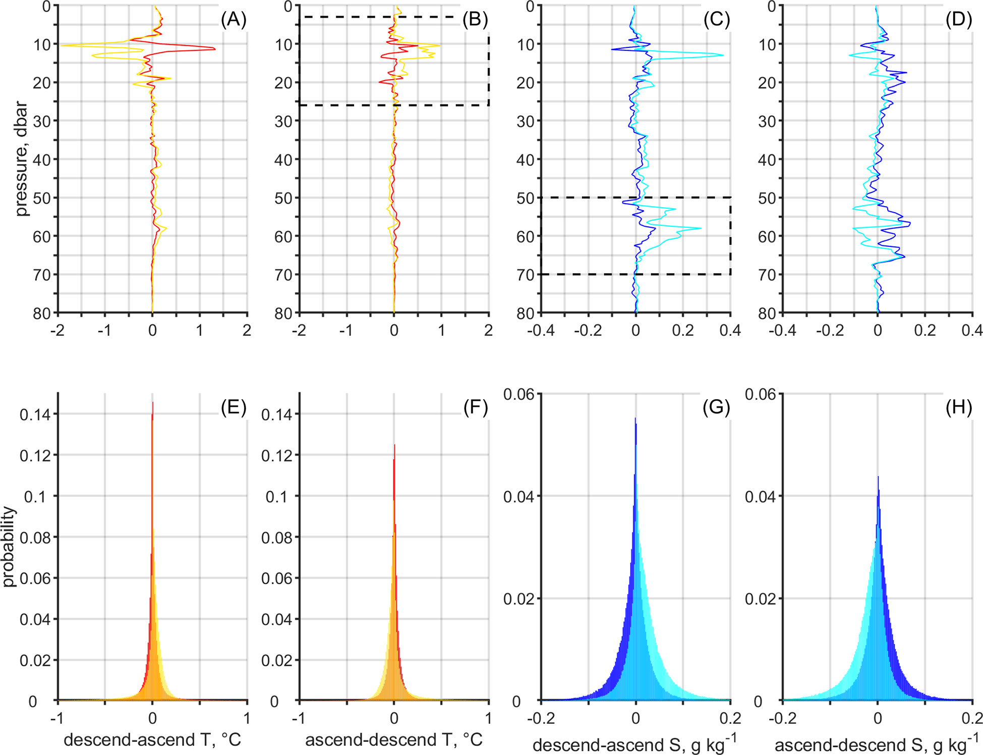
Figure 11 (A–D) The discrepancy respectively between two consecutive temperature and salinity profiles as shown in Figures 9A–D). The dashed line in the upper part of the water column highlights the thermocline range (B) and in the lower part the halocline range (C). (E–H) The histogram of discrepancies respectively for all the compared temperature (raw in yellow and corrected in red) and salinity (raw in cyan and corrected in blue) profiles in case of descend-ascend and ascend-descend.

To compensate for the thermal lag of the CTD, combinations of α_tl (from 0.025 to 0.1 by 0.025) and τ_tl (from 9 to 14 s by 0.5 s) were applied to the temperature data to derive salinity. The optimal coefficients were chosen by comparing temperature-salinity diagrams similarly as was done for response time. The median value of the mean area was expected to be smaller than the ones calculated based on the raw data (Figures 10C, D). In this study, the satisfying result was obtained in the case of α_tl = 0.0625 and τ_tl = 11.5s. Figures 9C, D shows examples of corrected salinity profile. Note that now the zoomed plot is the case descend–ascend. Figures 11C, D shows the discrepancy between two consecutive profiles shown in Figures 9C, D. The profiles show better agreement in case of descend-ascend because the data in the halocline range is measured with little time separation. Figures 11G, H shows the histogram of discrepancies for all the compared profiles. The discrepancies between profiles were improved after calculating salinity with reassessed temperature.

Data availability statement

The datasets presented in this study can be found in online repositories. The names of the repository/repositories and accession number(s) can be found below: https://doi.org/10.17882/84802 SEANOE.

Author contributions

KS was responsible for processing and analyzing the glider data and writing the paper. UL contributed to the analysis setup and writing the paper. TL contributed to writing the paper. All authors participated in designing the survey and piloting the glider. All authors contributed to the article and approved the submitted version.

Funding

This work was supported by the Estonian Research Council grant (PRG602) and institutional research funding (IUT-19-6) of the Estonian Ministry of Education and Research.

Acknowledgments

We would like to thank our colleagues and the crew of RV Salme for their assistance during the deployment and recovery of the glider.

Conflict of interest

The authors declare that the research was conducted in the absence of any commercial or financial relationships that could be construed as a potential conflict of interest.

Publisher’s note

All claims expressed in this article are solely those of the authors and do not necessarily represent those of their affiliated organizations, or those of the publisher, the editors and the reviewers. Any product that may be evaluated in this article, or claim that may be made by its manufacturer, is not guaranteed or endorsed by the publisher.

Supplementary material

The Supplementary Material for this article can be found online at: https://www.frontiersin.org/articles/10.3389/fmars.2023.984246/full#supplementary-material

References

Alenius P., Myrberg K., Nekrasov A. (1998). The physical oceanography of the gulf of Finland: a review. Boreal Environ. Res. 3, 97–125.

Google Scholar

Alenius P., Nekrasov A., Myrberg K. (2003). Variability of the baroclinic rossby radius in the gulf of Finland. Continent. Shelf Res. 23 (6), 563–573. doi: 10.1016/S0278-4343(03)00004-9

CrossRef Full Text | Google Scholar

Bishop C. M. (2008). Sensor dynamics of autonomous underwater gliders (master’s thesis) (Canada: Memorial University of Newfoundland). Available at: http://research.library.mun.ca/id/eprint/9330. Retrieved from Memorial University Research Repository.

Google Scholar

Boccaletti G., Ferrari R., Fox-Kemper B. (2007). Mixed layer instabilities and restratification. J. Phys. Oceanogr. 37 (9), 2228–2250. doi: 10.1175/JPO3101.1

CrossRef Full Text | Google Scholar

Buckingham C. E., Lucas N. S., Belcher S. E., Rippeth T. P., Grant A. L. M., Lesommer J., et al. (2019). The contribution of surface and submesoscale processes to turbulence in the open ocean surface boundary layer. 11 (12), 4066–4094. doi: 10.1029/2019MS001801

PubMed Abstract | CrossRef Full Text | Google Scholar

Callies J., Ferrari R. (2013). Interpreting energy and tracer spectra of upper-ocean turbulence in the submesoscale range (1–200 km). J. Phys. Oceanogr. 43 (11), 2456–2474. doi: 10.1175/JPO-D-13-063.1

CrossRef Full Text | Google Scholar

Callies J., Ferrari R., Klymak J. M., Gula J. (2015). Seasonality in submesoscale turbulence. Nat. Commun. 6, 6862. doi: 10.1038/ncomms7862

PubMed Abstract | CrossRef Full Text | Google Scholar

Carpenter J. R., Rodrigues A., Schultze L. K. P., Merckelbach L., Suzuki N., Baschek B., et al. (2020). Shear instability and turbulence within a submesoscale front following a storm. Geophys. Res. Lett. 47 (23), e2020GL090365. doi: 10.1029/2020GL090365

CrossRef Full Text | Google Scholar

Charney J. G. (1971). Geostrophic turbulence. J. Atmos. Sci. 28 (6), 1087–1095. doi: 10.1175/1520-0469(1971)028<1087:GT>2.0.CO;2

CrossRef Full Text | Google Scholar

Cole S., Rudnick D. L. (2012). The spatial distribution and annual cycle of upper ocean thermohaline structure. J. Geophys. Res. Atmos. 117 (C2), C02027. doi: 10.1029/2011JC007033

CrossRef Full Text | Google Scholar

de Verneil A., Franks P. J. S., Ohman M. D. (2019). Frontogenesis and the creation of fine-scale vertical phytoplankton structure. J. Geophys. Res.: Oceans 124, 1509–1523. doi: 10.1029/2018JC014645

CrossRef Full Text | Google Scholar

du Plessis M., Swart S., Ansorge I. J., Mahadevan A. (2017). Submesoscale processes accelerate seasonal restratification in the subantarctic ocean. J. Geophys. Res.: Oceans 122 (4), 2960–2975. doi: 10.1002/2016JC012494

CrossRef Full Text | Google Scholar

du Plessis M., Swart S., Ansorge I. J., Mahadevan A., Thompson A. F. (2019). Southern ocean seasonal restratification delayed by submesoscale wind–front interactions. J. Phys. Oceanogr. 49 (4), 1035–1053. doi: 10.1175/JPO-D-18-0136.1

CrossRef Full Text | Google Scholar

Ferrari R., Boccaletti G. (2004). Eddy-mixed layer interactions in the ocean. Oceanography 17 (3), 12–21. doi: 10.5670/oceanog.2004.26

CrossRef Full Text | Google Scholar

Fox-Kemper B., Ferrari R., Hallberg R. (2008). Parameterization of mixed layer eddies. part I: Theory and diagnosis. J. Phys. Oceanogr. 38, 1145–1165. doi: 10.1175/2007JPO3792.1

CrossRef Full Text | Google Scholar

Garau B., Ruiz S., Zhang W. G., Pascual A., Heslop E., Kerfoot J., et al. (2010). Thermal lag correction on Slocum CTD glider data. J. Atmos. Ocean. Technol. 28 (9), 1065–1071. doi: 10.1175/JTECH-D-10-05030.1

CrossRef Full Text | Google Scholar

Garcia-Jove M., Mourre B., Zarokanellos N. D., Lermusiaux P. F. J., Rudnick D. L., Tintoré J. (2022). Frontal dynamics in the alboran Sea: 2. processes for vertical velocities development. J. Geophys. Res.: Oceans 127, e2021JC017428. doi: 10.1029/2021JC017428

CrossRef Full Text | Google Scholar

Giddy I., Swart S., du Plessis M., Thompson A. F., Nicholson S.-A. (2021). Stirring of sea-ice meltwater enhances submesoscale fronts in the southern ocean. J. Geophys. Res.: Oceans 126, e2020JC016814. doi: 10.1029/2020JC016814

CrossRef Full Text | Google Scholar

Hersbach H., Bell B., Berrisford P., Biavati G., Horányi A., Muñoz Sabater J., et al. (2022)ERA5 hourly data on single levels from 1979 to present. Copernicus climate change service (C3S) climate data store (CDS) (Accessed JAN-2022).

Google Scholar

Hersbach H., Bell B., Berrisford P., Hirahara S., Horányi A., Muñoz-Sabater J., et al. (2020). The ERA5 global reanalysis. Q. J. R. Meteorol. Soc. 146, 1999–2049. doi: 10.1002/qj.3803

CrossRef Full Text | Google Scholar

Hoskins B. J. (1974). The role of potential vorticity in symmetric stability and instability. Q. J. R. Meteorol. Soc. 100, 480–482. doi: 10.1002/qj.49710042520

CrossRef Full Text | Google Scholar

IOC, SCOR and IAPSO. (2010). The international thermodynamic equation of seawater – 2010: Calculation and use of thermodynamic properties. Intergovernmental Oceanographic Commission, Manuals and Guides No. 56, Paris: UNESCO (English), 196 pp. Available at: https://www.teos-10.org/pubs/TEOS-10_Manual.pdf.

Google Scholar

Jaeger G. S., MacKinnon J. A., Lucas A. J., Shroyer E., Nash J., Tandon A., et al. (2020). How spice is stirred in the bay of Bengal. J. Phys. Oceanogr. 50 (9), 2669–2688. doi: 10.1175/JPO-D-19-0077.1

CrossRef Full Text | Google Scholar

Karimova S., Gade M. (2016). Improved statistics of sub-mesoscale eddies in the Baltic Sea retrieved from SAR imagery. Int. J. Remote Sens. 37 (10), 2394–2414. doi: 10.1080/01431161.2016.1145367

CrossRef Full Text | Google Scholar

Karstensen J., Liblik T., Fischer J., Bumke K., Krahmann G. (2014). Summer upwelling at the boknis eck time-series station, (1982 to 2012) – a combined glider and wind data analysis. Biogeosciences 11, 3603–3617. doi: 10.5194/bg-11-3603-2014

CrossRef Full Text | Google Scholar

Keevallik S., Soomere T. (2014). Regime shifts in the surface-level average air flow over the gulf of Finland during 1981-2010. Proc. Estonian Acad. Sci. 63 (4), 428–437. doi: 10.3176/proc.2014.4.08

CrossRef Full Text | Google Scholar

Kikas V., Lips U. (2016). Upwelling characteristics in the gulf of Finland (Baltic Sea) as revealed by ferrybox measurements in 2007–2013. Ocean Sci. 12 (6), 2863–2898. doi: 10.5194/osd-12-2863-2015

CrossRef Full Text | Google Scholar

Kunze E., Klymak J. M., Lien R.-C., Ferrari R., Lee C. M., Sundermeyer M. A., et al. (2015). Submesoscale Water-Mass Spectra in the Sargasso Sea J. Phys. Oceanogr. 45 (5), 1325–1338. doi: 10.1175/JPO-D-14-0108.1

CrossRef Full Text | Google Scholar

Lapeyre G., Klein P., Hua B. L. (2006). Oceanic restratification forced by surface frontogenesis. J. Phys. Oceanogr. 36 (8), 1577–1590. doi: 10.1175/JPO2923.1

CrossRef Full Text | Google Scholar

Large W. G., Pond S. (1981). Open ocean momentum flux measurements in moderate to strong winds. J. Phys. Oceanogr. 11 (3), 324–336. doi: 10.1175/1520-0485(1981)011<0324:OOMFMI>2.0.CO;2

CrossRef Full Text | Google Scholar

Lehmann A., Myrberg K., Höflich K. (2012). A statistical approach to coastal upwelling based on the analysis of satellite data for 1990–2009. Oceanologia 54 (3), 369–393. doi: 10.5697/oc.54-3.369

CrossRef Full Text | Google Scholar

Liblik T., Lips U. (2017). Variability of pycnoclines in a three-layer, large estuary: the gulf of Finland. Boreal Environ. Res. 22, 27–47.

Google Scholar

Liblik T., Väli G., Salm K., Laanemets J., Lilover M.-J., Lips U. (2022). Quasi-steady circulation regimes in the Baltic Sea. Ocean Sci. 18(3), 857–879. doi: 10.5194/os-18-857-2022

CrossRef Full Text | Google Scholar

Lips U., Kikas V., Liblik T., Lips I. (2016). Multi-sensor in situ observations to resolve the sub-mesoscale features in the stratified gulf of Finland, Baltic Sea. Ocean Sci. 12 (3), 715–732. doi: 10.5194/os-12-715-2016

CrossRef Full Text | Google Scholar

Lips I., Lips U. (2017). The importance of mesodinium rubrum at post-spring bloom nutrient and phytoplankton dynamics in the vertically stratified Baltic Sea. Front. Mar. Sci. 4. doi: 10.3389/fmars.2017.00407

CrossRef Full Text | Google Scholar

Lips I., Rünk N., Kikas V., Meerits A., Lips U. (2014). High-resolution dynamics of spring bloom in the gulf of Finland, Baltic Sea. J. Mar. Syst. 129, 135–149. doi: 10.1016/j.jmarsys.2013.06.002

CrossRef Full Text | Google Scholar

Mahadevan A., Tandon A., Ferrari R. (2010). Rapid changes in mixed layer stratification driven by submesoscale instabilities and winds. J. Geophys. Res. Atmos. 115 (C3), C03017. doi: 10.1029/2008JC005203

CrossRef Full Text | Google Scholar

McDougall T., Barker P. M. (2011). Getting started with TEOS-10 and the Gibbs Seawater (GSW) Oceanographic Toolbox, 28pp., SCOR/IAPSO WG127, ISBN 978-0-646-55621-5." Available at: https://www.teos-10.org/software.htm.

Google Scholar

McWilliams J. C. (2016). “Submesoscale currents in the ocean,” in . Proc. R. Soc. A., Vol. 472(2189):20160117. doi: 10.1098/rspa.2016.0117

CrossRef Full Text | Google Scholar

Mensah V., Menn M. L., Morel Y. (2009). Thermal mass correction for the evaluation of salinity. J. Atmos. Ocean. Technol. 26 (3), 665–672. doi: 10.1175/2008JTECHO612.1

CrossRef Full Text | Google Scholar

Meyer D., Lips U., Prien R. D., Naumann M., Liblik T., Schuffenhauer I., et al. (2018). Quantification of dissolved oxygen dynamics in a semi-enclosed sea - a comparison of observational platforms. Continent. Shelf Res. 169, 34–45. doi: 10.1016/j.csr.2018.09.011

CrossRef Full Text | Google Scholar

Myrberg K., Andrejev O. (2003). Main upwelling regions in the Baltic Sea – a statistical analysis based on three-dimensional modeling. Boreal Environ. Res. 8, 97–112.

Google Scholar

Pavelson J., Laanemets J., Kononen K., Nõmman S. (1997). Quasipermanent density front at the entrance to the gulf of Finland: Response to wind forcing. Continent. Shelf Res. 17, 253–265. doi: 10.1016/S0278-4343(96)00028-3

CrossRef Full Text | Google Scholar

Pérez J. G. C., Pallàs-Sanz E., Tenreiro M., Meunier T., Jouanno J., Ruiz-Angulo A. (2022). Overturning instabilities across a warm core ring from glider observations. J. Geophys. Res.: Oceans 127, e2021JC017527. doi: 10.1029/2021JC017527

CrossRef Full Text | Google Scholar

Pietri A., Testor P., Echevin V., Chaigneau A., Mortier L., Eldin G., et al. (2013). Finescale vertical structure of the upwelling system off southern Peru as observed from glider data. J. Phys. Oceanogr. 43 (3), 631–646. doi: 10.1175/JPO-D-12-035.1

CrossRef Full Text | Google Scholar

Rubio A., Bosch D. G., Jordà G., Infantes M. E. (2009). Estimating geostrophic and total velocities from CTD and ADCP data: intercomparison of different methods. J. Mar. Syst. 77 (1), 61–76. doi: 10.1016/j.jmarsys.2008.11.009

CrossRef Full Text | Google Scholar

Rudnick D. L., Cole S. (2011). On sampling the ocean using underwater gliders. J. Geophys. Res. 116 (C8), C08010. doi: 10.1029/2010JC006849

CrossRef Full Text | Google Scholar

Spall M. A. (1995). Frontogenesis, subduction, and cross-front exchange at upper ocean fronts. J. Geophys. Res. 100 (C2), 2543–2557. doi: 10.1029/94JC02860

CrossRef Full Text | Google Scholar

Swart S., Thomalla S. J., Monteiro P. M. S. (2015). The seasonal cycle of mixed layer dynamics and phytoplankton biomass in the Sub-Antarctic zone: A high-resolution glider experiment. J. Mar. Syst. 147 (15), 103–115. doi: 10.1016/j.jmarsys.2014.06.002

CrossRef Full Text | Google Scholar

Taylor J., Ferrari R. (2009). On the equilibration of a symmetrically unstable front via a secondary shear instability. J. Fluid Mech. 622, 103–113. doi: 10.1017/S0022112008005272

CrossRef Full Text | Google Scholar

Taylor J. R., Ferrari R. (2010). Buoyancy and wind-driven convection at mixed layer density fronts. J. Phys. Oceanogr. 40 (6), 1222–1242. doi: 10.1175/2010JPO4365.1

CrossRef Full Text | Google Scholar

Thomas L. N. (2005). Destruction of potential vorticity by winds. J. Phys. Oceanogr. 35 (12), 2457–2466. doi: 10.1175/JPO2830.1

CrossRef Full Text | Google Scholar

Thomas L., Ferrari R. (2008). Friction, frontogenesis, and the stratification of the surface mixed layer. J. Phys. Oceanogr. 38 (11), 2501. doi: 10.1175/2008JPO3797.1

CrossRef Full Text | Google Scholar

Thomas L., Tandon A., Mahadevan A. (2008). Submesoscale processes and dynamics. Washington DC Am. Geophys. Union Geophys. Monogr. Ser. 177, 17–38. doi: 10.1029/177GM04

CrossRef Full Text | Google Scholar

Thomas L. N., Taylor J. R., Ferrari R., Joyce M. T. (2013). Symmetric instability in the gulf stream. Deep Sea Res. Part II: Topical Stud. Oceanogr. 91, 96–110. doi: 10.1016/j.dsr2.2013.02.025

CrossRef Full Text | Google Scholar

Thompson A. F., Lazar A., Buckingham C., Naveira Garabato A. C., Damerell G. M., Heywood K. J. (2016). Open-ocean submesoscale motions: A full seasonal cycle of mixed layer instabilities from gliders. J. Phys. Oceanogr. 46 (4), 1285–1307. doi: 10.1175/JPO-D-15-0170.1

CrossRef Full Text | Google Scholar

Tuomi L., Myrberg K., Lehmann A. (2012). The performance of the parameterisations of vertical turbulence in the 3D modelling of hydrodynamics in the Baltic Sea. Continent. Shelf Res. 50/51, 64–79. doi: 10.1016/j.csr.2012.08.007

CrossRef Full Text | Google Scholar

Väli G., Zhurbas V., Lips U., Laanemets J. (2017). Submesoscale structures related to upwelling events in the gulf of Finland, Baltic Sea (numerical experiments). J. Mar. Syst. 171 (1), 31–42. doi: 10.1016/j.jmarsys.2016.06.010

CrossRef Full Text | Google Scholar

Wortham C., Wunsch C. (2014). A multidimensional spectral description of ocean variability. J. Phys. Oceanogr. 44 (3), 944–966. doi: 10.1175/JPO-D-13-0113.1

CrossRef Full Text | Google Scholar

Ylöstalo P., Seppälä J., Kaitala S., Maunula P., Simis S. (2016). Loadings of dissolved organic matter and nutrients from the Neva river into the gulf of Finland – biogeochemical composition and spatial distribution within the salinity gradient. Mar. Chem. 186, 58–71. doi: 10.1016/j.marchem.2016.07.004

CrossRef Full Text | Google Scholar

Yu X., Naveira Garabato A. C., Martin A. P., Evans D. G., Su Z. (2019b). Wind-forced symmetric instability at a transient mid-ocean front. Geophys. Res. Lett. 46 (11), 281–11, 291. doi: 10.1029/2019GL084309

CrossRef Full Text | Google Scholar

Yu X., Naviera Garabato A. C., Martin A., Buckingham C., Brannigan L., Su Z. (2019a). An annual cycle of submesoscale vertical flow and restratification in the upper ocean. J. Phys. Oceanogr. 49 (6), 1439–1461. doi: 10.1175/JPO-D-18-0253.1

CrossRef Full Text | Google Scholar

Zhurbas V., Väli G., Kostianoy A. G., Lavrova O. (2019). Hindcast of the mesoscale eddy field in the southeastern Baltic Sea: Model output vs satellite imagery. Russian J. Earth Sci. 19 (4), 1–17. doi: 10.2205/2019ES000672

CrossRef Full Text | Google Scholar