Seismic airgun sound propagation in shallow water of the East Siberian shelf and its prediction with the measured source signature

Seismic airgun sound was measured with an autonomous passive acoustic recorder as a function of distance from 18.6 to 164.2 km in shallow water (<70 m) at the continental shelf of the East Siberian Sea in September 2019. The least-square regression curves were derived in the zero-to-peak sound pressure level, sound exposure level, and band level in a frequency range between 10 and 300 Hz using the initial amplitude scaled from the near-field hydrophone data. In addition, propagation modeling based on the parabolic equation with the measured source spectrum was performed for range-dependent bathymetry, and the results were compared with the band level of the measurements. The sediment structure of the measurement area was a thin layer of iceberg-scoured postglacial mud overlying a fast bottom with high density based on grounding events of past ice masses. The observed precursor arrivals, modal dispersion, and rapid decrease in spectrum level at low frequencies can be explained by the condition of the high-velocity sediment. Our results can be applied to studies on the inversion of ocean boundary conditions and measurement geometry and basic data for noise impact assessment.

1 Introduction

Seismic surveys have been conducted for natural resource exploration and geoscientific investigation. The seismic wave produced by airgun arrays towed behind a research vessel is one of the representative anthropogenic noise sources with extremely high sound pressure levels at low frequencies. The source levels of airgun arrays are estimated to be 200–260 dB re 1μPa at the zero-to-peak sound pressure level and 186–228 dB re 1μPa²s at the sound exposure level, although they may vary with airgun type, operating scheme, and anisotropic radiation pattern (Caldwell and Dragoset, 2000; Thode et al., 2010; Hermannsen et al., 2015; Gisiner, 2016; Duncan et al., 2017; Martin et al., 2017; van der Schaar et al., 2017; Kavanagh et al., 2019). Airgun pulses reflected from the seafloor and subsurface interface between two sedimentary layers with different densities and velocities (i.e., acoustic impedance) are received at a streamer corresponding to hydrophone line array lengths of up to several km; then, the geological structure below the seafloor is shown as an image. The sea surface-reflected path of an airgun pulse, which is typically generated close to the sea surface at a depth of 5–15 m, is produced sequentially after the direct path with a perfectly negative phase as a mirror source. Due to the arrival time difference from the direct path, the sea surface-reflected path causes frequency nullings in the received spectral shape, which are referred to as “ghost notch” (Caldwell and Dragoset, 2000; Prior et al., 2021).

Different types of compressed air sources have been used over the past few decades (Ziolkowski, 1970; Krail, 2010; Gisiner, 2016). The generator-injector (GI) airgun, developed in 1989, consists of two air chambers instead of one (Pascouet, 1991). The waveform generated from this airgun is characterized by a clear primary pulse and a high primary-to-bubble ratio using the extra air of the injector with a time delay (Landrø, 1992; Krail, 2010). The injection mechanism reduces residual bubble oscillations to improve the seismic data quality. Bubble oscillations can also be reduced by using airgun arrays. The use of a single airgun is rare, and dozens of airguns have been used in the field (Gisiner, 2016). Airgun arrays also produce a beam pattern in a vertically downward direction and increase the source level, which is an important factor for acquiring accurate and deep stratigraphic images. The energy output of the airgun array is linearly proportional to the number of guns, the firing pressure, and the cube root of the volume of the array (Dragoset, 1990; Dragoset, 2000).

Studies on predictions of source signatures and underwater propagation have been conducted (e.g., International Airgun Modeling Workshop). Ziolkowski predicted the amplitude of the source signature based on Gilmore’s equation in 1970, and the prediction methods for near-field signatures have been extensively developed and well matched with measurements (Ziolkowski et al., 1982; Landrø et al., 1991; Laws et al., 1998). In addition, several models for predicting propagation characteristics are being developed, such as Cagam, Gundalf, Nucleus and AAMS (Alexander, 2000; Gisiner, 2016; Ainslie et al., 2019; Duncan and Gavrilov, 2019). Propagation prediction over long distances has been conducted with numerical models based on the parabolic equation, normal mode, wavenumber integration, and ray theory, including some of the models mentioned above (Hovem et al., 2012; Duncan et al., 2013; Koessler et al., 2017; Ainslie et al., 2019; Heaney and Campbell, 2019). Seismic airgun sound, which is dominant at frequencies below ~125 Hz (Caldwell and Dragoset, 2000; Heaney and Campbell, 2019), interacts with ocean boundaries and shows acoustic characteristics depending on the sediment type, water depth, and sound speed profile (Duncan et al., 2013; Ainslie et al., 2016; Martin et al., 2017; Abadi and Freneau, 2019). Therefore, acoustic interpretations of airgun sound propagation that incorporate knowledge of the operating scheme and the ocean environment are needed.

In this study, we focus on airgun sound propagation in shallow water on the East Siberian Shelf, which has rarely been studied from geological and hydroacoustic perspectives. The East Siberian Shelf is a region where the distribution of subsea permafrost has been reported (Brown et al., 1997; Romanovskii, 2004). Mega-scale glacial lineations and moraine ridges observed at the East Siberian-Chukchi continental margin indicate widespread grounding events of southern-sourced large-scale ice masses (i.e., ice sheets) during glacial periods (Hegewald and Jokat, 2013; Niessen et al., 2013; Dove et al., 2014; Kim et al., 2021). The surficial layer is covered with relatively soft, unconsolidated sediments in the form of iceberg-scoured postglacial sediments overlying the cemented subsurface sediment (O'Regan et al., 2017; Jin, 2020). The acoustic characteristics of airgun sound, such as the effect of the cutoff frequency, precursor arrival, and modal dispersion, can be observed under these conditions and can be described by normal mode theory (Frisk, 1994; Jensen, 2011; Landrø and Hatchell, 2012; Duncan et al., 2013; Keen et al., 2018). Therefore, we discuss acoustic characteristics based on the measurements of surficial sediment core data and multibeam images. However, we cannot obtain geoacoustic parameters from the deep subbottom structure, so we suggest that the lower layer could consist of a fast bottom based on the geological history of the region. This paper is the first to use a waveform measured at a near-field hydrophone, which has been typically used for only the quality control of airgun firing, to predict airgun sound propagation as the source spectrum in the numerical model. In addition, the ship tracks of the survey vessel moved approximately 150 km in a constant direction and at a constant speed, making the recorded airgun sound ideal acoustic data to study sound propagation. Our results can be used to understand the variations in the acoustic environment of the Arctic Ocean due to increased anthropogenic noise with a warming Arctic climate. In other words, Arctic sea-ice reduction, leading to increased human activities such as shipping and seismic surveys, contributes to a wealth of new scientific data (Kim et al., 2021); however, changes in the underwater acoustic environment due to anthrophony can affect the growth, survival, reproduction, communication, and habitat diversity of marine life (Slabbekoorn et al., 2010; Hawkins and Popper, 2017).

2 Methods

2.1 Moored autonomous acoustic recorder and multichannel seismic survey

An autonomous passive acoustic recorder (AURAL-M2, Multi-Electronique Inc.) was moored in the East Siberian Shelf (74° 37.327’N, 174° 56.397’E) at a depth of 57 m, corresponding to 13 m above the seafloor (Figure 1A and Figure 2A). AURAL-M2 was set to record acoustic data for 10 minutes every hour with a 16-bit resolution and a 32,768 Hz sampling rate. The receiving voltage sensitivity of the hydrophone is −165 dB re 1V/μPa and almost flat with a ± 2 dB error in the frequency range of 10 Hz to 10 kHz (De Robertis and Wilson, 2011). AURAL-M2, deployed in August 2019, recorded the acoustic data for one year. Among the one-year recordings, the acoustic data from 18:00 on 9 September to 11:10 on 10 September were used in the analysis.

FIGURE 1

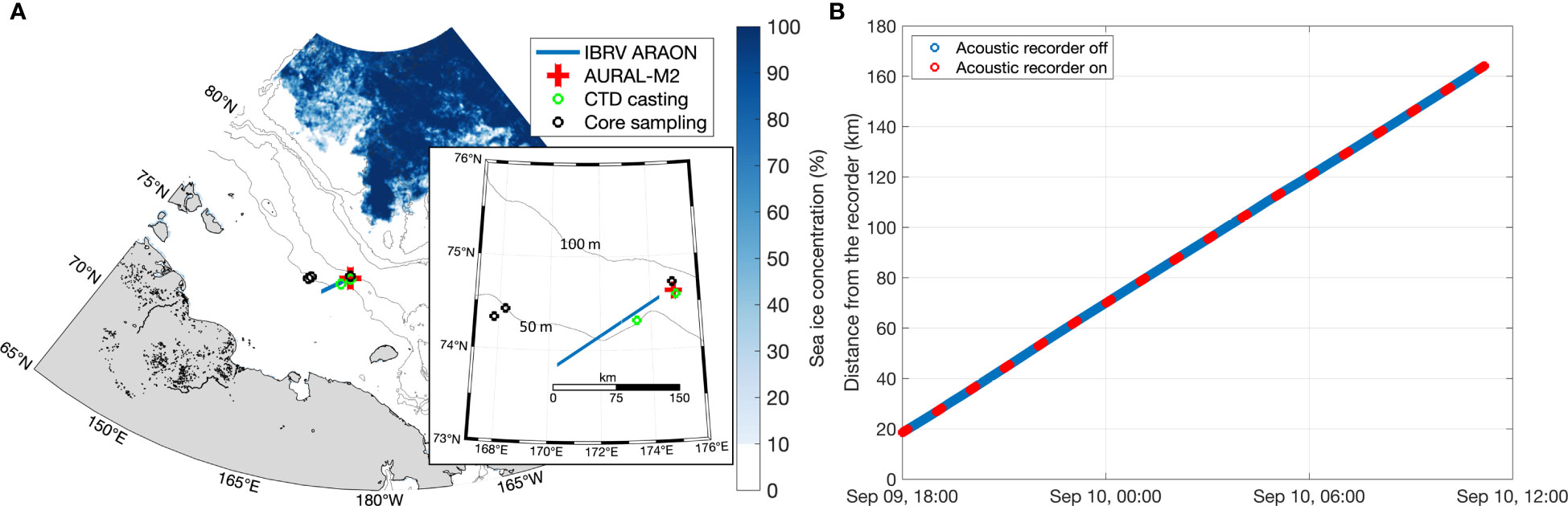
Figure 1 (A) Map of the measurement area with the sea ice concentration on 9 September showing the AURAL-M2 mooring location (red cross), seismic survey track (blue line), two CTD casting sites (green circles) and three core sampling sites (black circles). (B) The distance from AURAL-M2 to IBRV ARAON. The distances for 10 minutes every hour when the AURAL-M2 was working are represented by red circles.

FIGURE 2

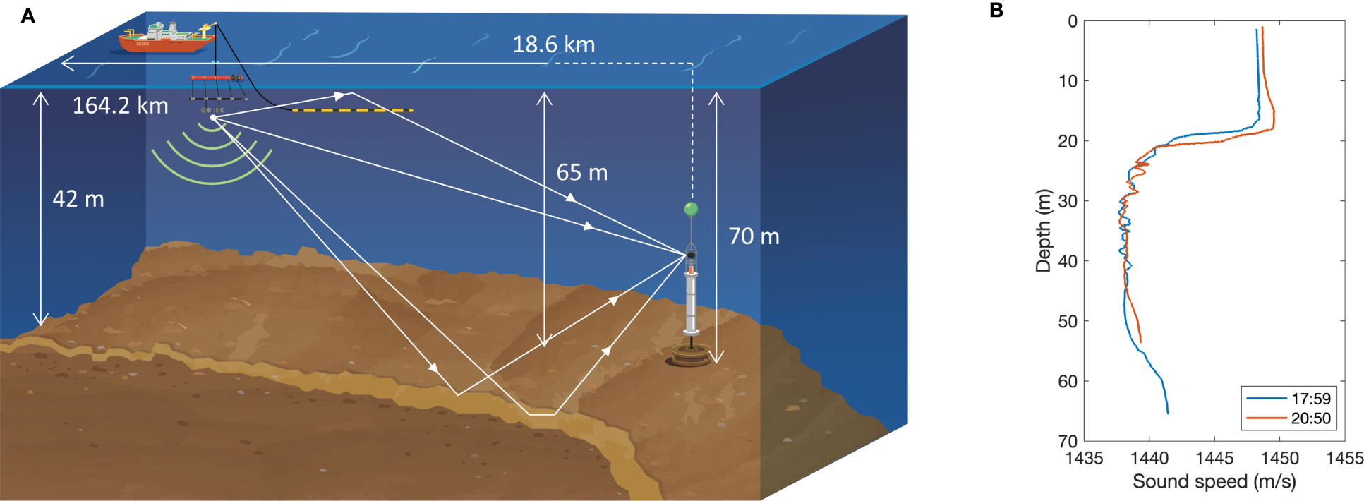
Figure 2 (A) The geometry of MCS airgun sound measurements. (B) Vertical sound speed profiles measured at 17:59 and 20:50 on 14 September.

The ice breaking research vessel (IBRV) ARAON multichannel seismic (MCS) survey was conducted in the Chukchi–East Siberian Continental Margin from 2 to 10 September 2019 (Jin, 2020). The ARAON approached AURAL-M2 from 02:54 on 9 September in a constant direction, and the closest point of approach (CPA) occurred at 15:47; then, the vessel moved away from AURAL-M2 until 18:24 on 10 September. Data from the transect where the distance increased from the CPA were used. The data from when the waveform was saturated at close distances from 16:00 to 17:10 on the 9^th and from when the signal-to-noise ratio was too small to detect from 12:00 to 18:00 on the 10^th were excluded from the analysis. A total of 1,017 airgun pulses were generated in the ARAON MCS system for 180 minutes. The distance from the firing location to AURAL-M2 was calculated using GPS data of ARAON MCS system (Figure 1B) and was verified using automatic identification system (AIS) data (Marine Traffic, 2019). The ship speed remained at 4.5 knots during the MCS survey, and the distance variations within 10 minutes ranged from 1.3 to 1.4 km (Jin, 2020). Two GI airguns (GI-SOURCE 355, Sercel) were arranged frontward and backward with an interplate distance of 2.5 m, and the total volume, working pressure, and pulse interval of the sources were 710 in³ (each 355 in³ volume; 250 and 105 in³ for the generator and injector, respectively), ~14 MPa, and ~10.8 sec, respectively (Jin, 2020). Two near-field hydrophones (AGH-7100-C, Geophysical Products Inc.) and two pressure sensors (AGH-D500, Geophysical Products Inc.) were placed at gunplates approximately 1 m above each airgun. The airgun firing depth was consistently 6 m. There was no sea ice during the MCS survey (Figure 1A), and the sea surface was calm with low waves and weak winds; therefore, there was no change in the firing depth records of the MCS system. Multibeam bathymetry data recorded during the MCS survey show that the water depth decreased from 65 m at the outer shelf to 42 m at the inner shelf (Figure 2A). The sound speed profile obtained from the conductivity-temperature-depth (CTD) data, measured on 14 September (green circles in Figure 1A), indicates a depth average of 1,442 m/s, with a range of 1,438 and 1,448 m/s (blue line in Figure 2B). The CTD data measured in the direction of the MCS survey track on the same day at a depth of 55 m exhibit a similar trend of sound speed profile (red line in Figure 2B). Surficial sediment cores were sampled at three depths of 73, 51 and 49 m in the 2021 research cruise (black circles in Figure 1A), and their mean grain sizes (MGS) were 6.7, 8.0, and 10.3 ϕ , respectively (where, ϕ=log₂(d/d₀) , d is the grain diameter, and d_o is a reference length of 1 mm, Supplementary Data 1.1 and Supplementary Figure 1).

2.2 Airgun pulse detection and analysis

Airgun pulses were detected by using matched filtering of a representative single pulse to recordings every 10 minutes (Han et al., 2021). Airgun sounds were quantified using three metrics: the zero-to-peak sound pressure level L_p, the sound exposure level L_E and the band level L_B calculated from acoustic data after a bandpass filter with a dominant frequency range between 10 and 300 Hz (Kinsler, 2000; ISO 18405, 2017). These are shown below:

$\begin{array}{ll}{L}_p=20{\log }_{10}(\frac{p_{\text{pk}}}{p_0})& (1)\end{array}$

$\begin{array}{ll}\begin{array}{}{L}_E,L_B=10{\text{log}}_{10}(\frac{E_p}{E_{p,0}})\text{where }{E}_p={\displaystyle {\int }_{t_1}^{t_2}{p}^2(t)dt}\end{array}& (2)\end{array}$

where p(t) and p_pk are the measured sound pressure and its peak absolute value, respectively. p₀=1μPa and E_p,0=1μPa²s are reference values of the sound pressure and the time-integrated squared sound pressure, respectively. t₁ and t₂ are the start and end points of the time window, respectively, for consideration of the exposure duration (ISO 18405, 2017; Han and Choi, 2022). The spectrum level was estimated using the sound exposure spectral density with units of dB re 1μPa²s/Hz (ISO 18405, 2017), which was computed from a single pulse of 4-sec duration with a fast Fourier transform (FFT) length of 32,768 points.

The waveform measured at the near-field hydrophone exhibited a spike-like signature and showed the direct path as a primary positive peak at 0.025 sec and the sea surface-reflected path as a relatively small negative peak at 0.032 sec (Figure 3A). The arrival time difference between the direct path and sea surface-reflected path was predicted to be ~7 ms based on the source-receiver geometry, and it was in close agreement with the measured waveform. Figure 3B illustrates the normalized amplitude-weighting spectrum calculated from the intensity average of 2,034 waveforms. Average curves were calculated from all data, which indicate a spectral peak at 27 Hz, and for the direct path only shown by the black dashed line, which was applied to the input of numerical propagation modeling in Section 2.3 (ISO 18405, 2017). The typical receiving voltage sensitivity of the near-field hydrophones is flat with ~ 7–7.5 V/bar (≈ -203 dB re 1V/μPa; AGH-7100-C, Geophysical Products Inc.). Two GI airguns released compressed air simultaneously, and near-field hydrophone signatures had an average peak of ~1.46 MPa. Landrø (1992) reported that GI airguns with volumes of 45 and 105 in³ produced peaks of approximately 0.16 and 0.22 MPa, respectively. In this study, the primary peak was predicted to be 0.56 MPa based on the relationship between the energy output and cube root of the generator volume. Because there was an unknown scaling factor in the analog-digital converter (Hotshot, Teledyne RTS), the sound pressure levels were calculated from near-field hydrophone signatures scaled by 0.38, resulting in a value close to the theoretically predicted value. L_p, L_E, and L_B were 235 dB re 1 μPa @ 1 m, 210 dB re 1 μPa²s @ 1 m, and 210 dB re 1 μPa²s @ 1 m, respectively, with standard deviations of 0.5, 0.7 and 0.7 dB, respectively, based on 2,034 pulses (Sound exposure level of 210 dB re 1 μPa²s @ 1 m equals sound exposure source level). L_E and L_B, calculated from signatures with or without the sea surface-reflected path, showed differences of 1.0 and 1.3 dB, respectively. This effect was not considered in this paper because scaled sound pressure levels were used. The sound pressure levels at a distance of 1 m were used as the starting point of the regression curves showing the decrement of airgun sound energy as a function of distance. The sound pressure level at a distance of 1 m could be replaced with the source level, which was expressed by two types of mean-square sound pressure level with a reference value of “1 μPa @ 1 m” and the time-integrated squared sound pressure level called the sound exposure source level with a reference value of “1 μPa²s @ 1 m” (ISO 18405, 2017). In this study, the zero-to-peak sound pressure level was used instead of the mean-square sound pressure level because the absolute peak value of the impulsive waveform is appropriate for the assessment of loudness in the time domain.

FIGURE 3

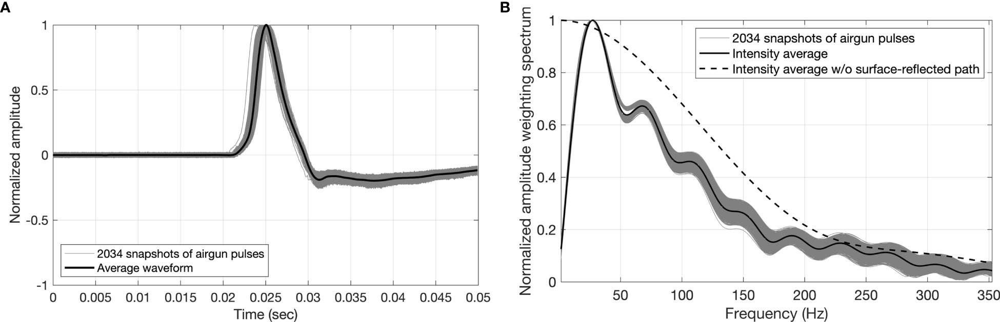
Figure 3 (A) Normalized waveforms of 2,034 airgun pulses (thin gray lines) measured at two near-field hydrophones and their ensemble average (thick black line). (B) Their normalized amplitude-weighting spectra. Black solid and dashed lines represent intensity average curves calculated with and without a surface-reflected path, respectively.

2.3 Propagation modeling of the airgun sound based on the parabolic equation

Airgun sound propagation was predicted using the broadband application of a range-dependent acoustic model (RAM), which is based on a parabolic equation (PE) and is appropriate for range-dependent bathymetry (Collins, 1993). The source and receiver positions were interchanged under the principle of reciprocity to consider the operating condition for a moving source and a fixed receiver in the propagation model. Because two airguns were used in our study, unlike the previous studies in which dozens of airguns were used, they can be considered a point source in the far-field region (Caldwell and Dragoset, 2000). The principle of reciprocity stipulates that the sound pressure at position B due to a source at position A is equal to the pressure at A due to a similar source at B. The principle is very general and valid in cases where the acoustic wave undergoes reflection and refraction at boundaries on its path from the source to the receiver (Hovem et al., 2012). The source depth was set to 57 m, and the acoustic field emitted from the source can be expressed as a function of frequency at the receiver position (r,z):

$\begin{array}{ll}p(r,z,f)=G(r,z,f)A(f)e^{-i\omega t}& (3)\end{array}$

where G(r,z,f) is Green’s function predicted by the RAM and ω is the angular frequency. A(f) is an amplitude-weighting spectrum corresponding to the normalized source spectrum shown in Figure 3B. Proper range step and depth grid spacing, as suggested by the relationship with the wavelength, were applied to the model inputs (Jensen, 2011), and their convergence tests were performed with steps corresponding to upper and lower frequencies. The input parameters applied for PE model prediction are listed in Supplementary Table 1. Because the integrated energy in the frequency range up to the first notch differs by less than 3 dB from that integrated higher than the first notch (Caldwell and Dragoset, 2000), the frequency band was considered to be between 10 Hz and 300 Hz with a 2 Hz bin. L_B in a given frequency bandwidth can be estimated using Parseval’s theorem (Ainslie, 2010; Dahl and Dall'Osto, 2017) as follows:

$\begin{array}{ll}{L}_B(r,z)=-10{\log }_{10}[\frac{1}{B}{{\displaystyle \int }}^{}p(r,z,f)p^{*}(r,z,f)df]+K& (4)\end{array}$

where B is the frequency bandwidth. The asterisk indicates a complex conjugate, and K is an offset constant. If the given bandwidth covers the entire airgun sound spectrum, the PE modeling output in L_B equals L_E.

The environmental conditions at the site, such as the sound speed profile in the water and bathymetry, were used as model inputs. We constructed a two-layer geoacoustic bottom model based on the collected core samples and the previous survey results. According to the core samples obtained from the SWERUS–C3 (SWERUS–C3: Swedish – Russian – US Arctic Ocean Investigation of Climate–Cryosphere–Carbon Interactions) expedition performed at a distance of approximately 430 km from our measurements in the East Siberian Shelf, the sound speed (c₁) and bulk density (ρ₁) of the surficial layer increased with depth within 1,471–1,590 m/s and 1.22–1.67 g/cm³ (O'Regan et al., 2017), respectively. The sound speed of 1,471 m/s in the surficial sediment was similar to that in the MGS of 6.7 ϕ sediment obtained from a core sample close to AURAL-M2 at the outer shelf (Ainslie, 2010). The lower layer was composed of an acoustically transparent material based on the subbottom profiler images in the SWERUS–C3 and those acquired simultaneously with the MCS survey (Jin, 2020). The sound speed (c₂) and density (ρ₂) measured from the core sample reaching some of the lower layer were approximately 1,590 m/s and 1.67 g/cm³, respectively (O'Regan et al., 2017), and they corresponded a sediment MGS of 3.8 ϕ (Ainslie, 2010). Consequently, the uppermost layer (layer-1) was set to the mud composed of soft unconsolidated sediments less than 4 m thick, and the lower layer (layer-2) was set to the diamicton with a thickness of 60 m (O'Regan et al., 2017; Jin, 2020). The acoustic properties of the sediment corresponding to the MGS in Ainslie (2010) are shown in Table 1. Because we could not find any data addressing acoustic properties over 10 ϕ , those of 9 ϕ , which is the most fine-grained value in Ainslie (2010), were used. Sound speeds, densities, and attenuation coefficients in layer-1, which corresponded to 6.7 ϕ at the outer shelf and 9.0 ϕ at the inner shelf, were linearly interpolated and range-dependently considered in the model (Table 1 and Supplementary Figure 2).

TABLE 1

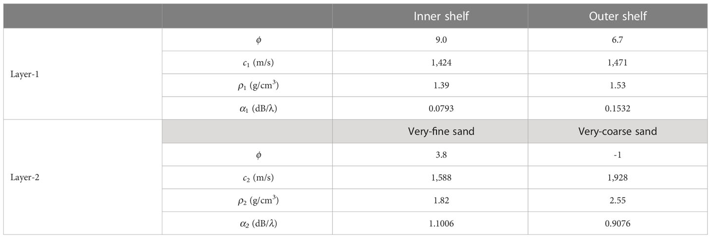
Table 1 Mean grain size (ϕ ), sound speeds (c), densities (p) and attenuations (α) applied in the two-layer bottom structure model.

3 Results

3.1 Acoustic characteristics of airgun pulses

The 180-minute acoustic data are shown by the waveform and spectrogram in Figures 4A, B. A total of 979 airgun pulses were detected over 54 pulses per 10 minutes, and their sound pressure levels in L_p and L_E decreased from 143 to 107 dB re 1μPa and from 132 to 99 dB re 1μPa²s, respectively, with distance (blue and red circles in Figure 5). Most of the undetected pulses spanned the beginning and end of the 10-minute recordings. The sound exposure spectral densities of airgun pulses and their average spectra are depicted by the thin gray lines and thick black lines, respectively, in Figure 4C. The spectrum levels from 10 to 300 Hz were relatively high, and the low-frequency energy below 50 Hz decreased rapidly from dark- to light-gray thin lines with increasing distance. This feature could be caused by the cutoff frequency in the shallow water waveguide, as will be discussed in Section 4. The ghost notch, which is twice the source depth divided by the sound speed in water, was observed near approximately 298 Hz (Caldwell and Dragoset, 2000). When the depth-averaged sound speed of 1,442 m/s was considered in this relationship, the airgun firing depth was estimated to be approximately 2.4 m, shallower than the actual firing depth of 6 m (Jin, 2020). The ghost notch is exactly determined by the reciprocal of the arrival time difference between the direct and surface-reflected path, and that of approximately 120 Hz is predicted at the firing depth of 6 m at a close distance. When the distance between source and receiver increases, the arrival time difference decreases, and high-frequency ghost notches may occur at the long distances (Landrø and Amundsen, 2018). The median sound exposure spectral densities of full acoustic data with and without airgun sounds are represented by blue and red solid lines in Figure 4C, which were taken from the intensity average of the mean-square sound pressure spectral densities estimated from the 1-minute segments compensated for the same time length of 4 sec as the airgun sound exposure spectral density. The airgun sound contributed to the increase in the ambient noise level by up to 13.8 dB re 1μPa²s/Hz at 39 Hz, and the effective frequency band between 10 and 800 Hz was similar to that in Han et al. (2021). Figures 4D, E show the waveform and spectrogram of a single pulse measured at the beginning of recordings. The 99% energy was concentrated within the duration of ~1.2 sec, and this length increased to 4 sec as the distance increased. A relatively weak amplitude early arrival was shown at approximately 4.6 sec, which will be discussed in Section 4.

FIGURE 4

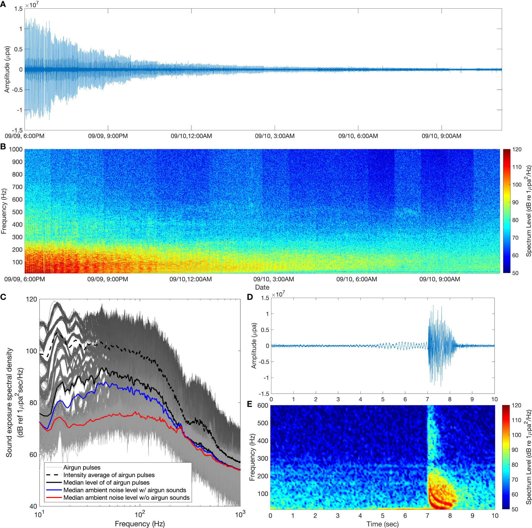
Figure 4 (A) Waveform and (B) spectrogram from 18:00 on 9 September to 11:10 on 10 September. Both are expressed by recorded acoustic data in a series of a 10-min recording and 50-min break schedule. (C) The sound exposure spectral densities of 979 pulses measured from short to long distances are expressed as dark- to light-gray thin lines. The intensity average and median spectrum levels are expressed as dashed and solid black lines, respectively. Median spectrum levels estimated from full acoustic data with and without airgun sound are represented by blue and red solid lines. (D) and (E) show the waveform and spectrogram of a single airgun pulse measured at the beginning of recording (8,192 fast Fourier transform points and 4,096-point Hanning window).

FIGURE 5

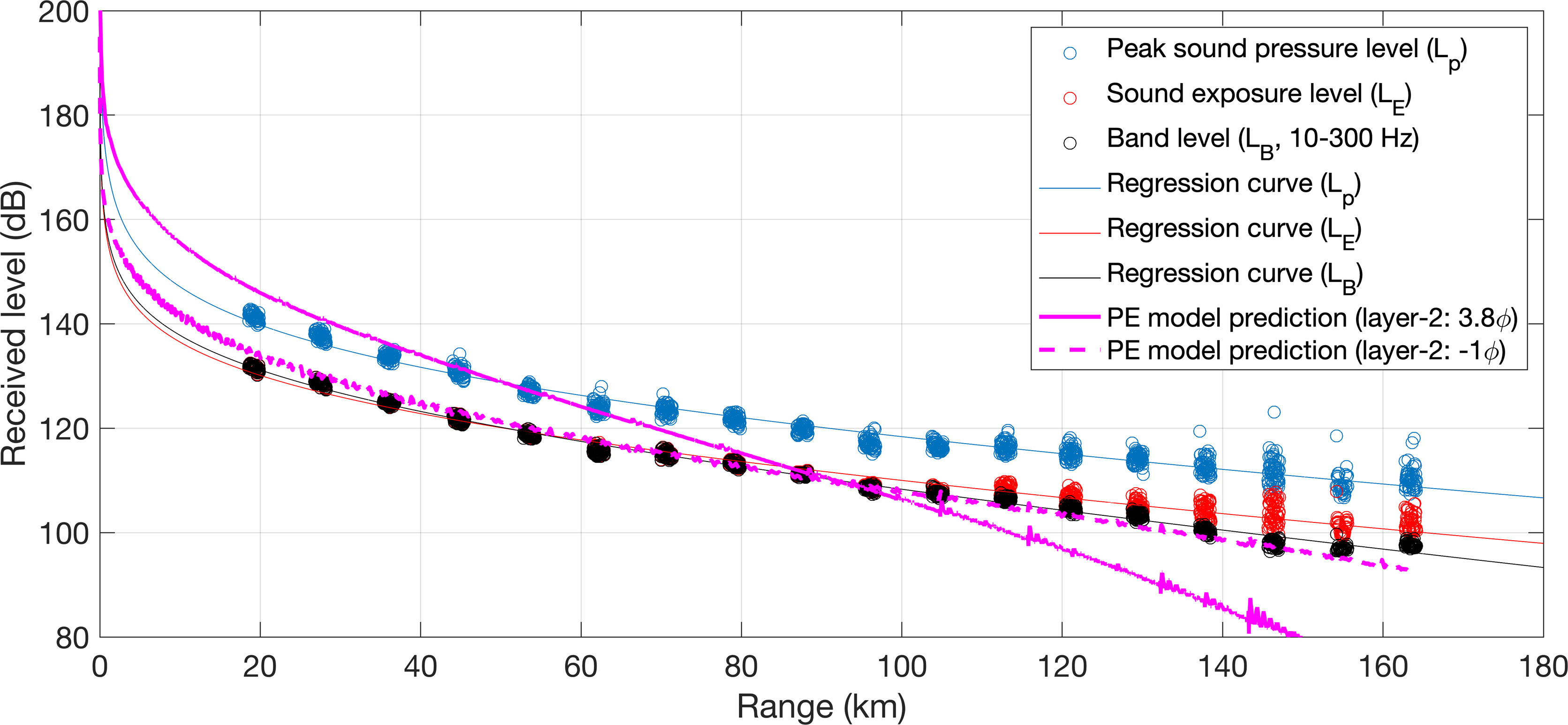
Figure 5 Received levels of airgun sound as a function of distance in L_p, L_E and L_B, which are represented by cyan, red, and black circles, respectively. Thin lines with the same colors depict the linear regression fitting curves using the least-squares method. Magenta solid and dashed lines show the PE model prediction curves when acoustic properties corresponding to 3.8 and -1 ϕ were applied, respectively.

3.2 Propagation of airgun sounds as a function of distance

Figure 5 shows the received levels of airgun pulses as a function of distance in L_p, L_E and L_B, respectively. L_E and L_B were approximately 9 dB lower than L_p, and they showed a difference of less than 1 dB until approximately 105 km. As the signal-to-noise ratio decreased with distance, L_p and L_E measured above 110 km were affected by the ambient noise at the out-of-airgun sound frequencies. The maximum standard deviations of the 18 distance groups in L_p and L_E were 2.5 and 2.2 dB, respectively, and L_B, which corresponded to the energy of airgun sound only, showed a maximum standard deviation of 0.6 dB.

When a sound source is a point source, sound propagation in water is a function of distance in the form of Nlog(r), where r is the distance in meters from a sound source and N is a spreading constant that depends on the ocean environment (Jensen, 2011). The regression curve of SL-Nlog(r)-ar was fit to the measurements, where SL represents the mean sound pressure levels referenced to 1 m calculated from the near-field hydrophone measurements in Section 2.2 and α is an attenuation coefficient. The two constants estimated by the regression curves are listed in Table 2. The prediction curve obtained using the PE model at a receiver depth of 6 m is shown by a thick magenta line. The root mean squared errors (RMSE) between measurements of L_B and predictions of the regression curve and PE model were 0.9 and 11.7 dB, respectively. The back-calculated SL from the PE model prediction was 218 dB, 8 dB higher than the sound pressure level of 210 dB calculated from the near-field hydrophone measurements. SL predicted from the PE model differs from that scaled from the measurements, and the reasons will be discussed in the next section.

TABLE 2

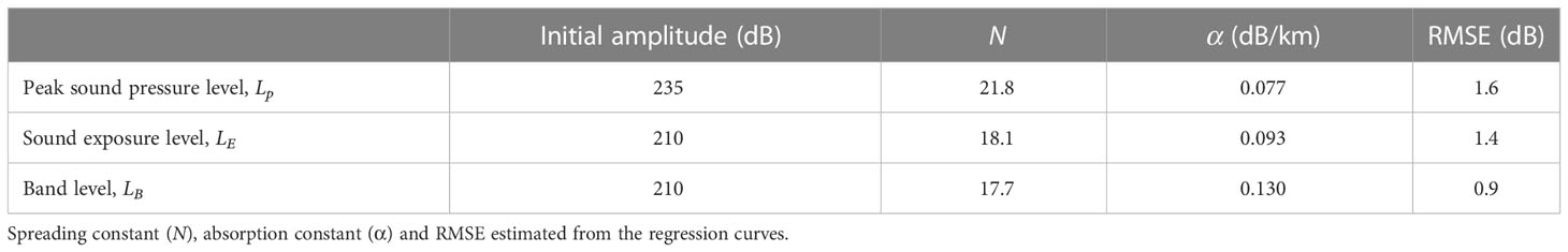
Table 2 Initial amplitude of regression curves for L_p, L_E and L_B which mean SPL calculated from the near-field hydrophone signature.

4 Discussion

The measurement region was shallow water less than 70 m with range-dependent bottom composition, although the change in water depth of 28 m is not large compared to the distance. Because the low-frequency airgun sounds are transmitted through deep and complex strata, the influence of sediment structure on sound propagation could be significant. Assuming a point source in shallow water, the spreading constant is close to 10, corresponding to cylindrical spreading (Jensen, 2011). However, the reason why the spreading constant derived from the regression curve in L_p was slightly greater than spherical spreading (N=20) and that in L_E and L_B was between spherical and cylindrical spreading is due to the range-dependent bathymetry and attenuation effect of the bottom boundary. The spreading constant could also vary with the unknown scaling factor, although the scaled amplitudes corresponding to the theoretical prediction were used as the initial value. The PE model prediction with reconstructed sediment structure was limited in consideration of acoustic properties of subseafloor sedimentary units and their surface structural topography. The reason why the back-calculated source level from the PE model prediction was 8 dB higher than that measured could be due to the same reason. Because PE model prediction curves using normalized amplitude-weighting spectra estimated from the direct path only and that with the surface-reflected path show similar trends, each with a root mean square error of 0.4 dB, the contribution of the sea surface-reflected path as the source spectrum could be ignored. In this section, we discuss the range-dependent propagation of airgun sounds. Then the application of inversely estimated geoacoustic properties in layer-2 based on the geological history of the region is considered.

Airgun sound increased the ambient noise level in a frequency range below 800 Hz and was dominant below approximately 300 Hz. Although the source spectrum indicates an energy peak of 27 Hz, the spectrum levels below 50 Hz rapidly decrease in Figure 4C due to the effect of the cutoff frequency. For a Pekeris waveguide, the cutoff frequency (f_c) of mode m is given by (Jensen, 2011)

$\begin{array}{ll}{f}_c=\frac{c(m-0.5)}{2h\sqrt{(1-{(\frac{c}{c_1})}^2)}}& (5)\end{array}$

where c and c₁ are the sound speeds in water and sediment, respectively, and h is water depth. When the sound speed in the sediment is higher than that in water, perfect trapping of the modes occur, and energy does not continually radiate out of the waveguide (Frisk, 1994). When the depth-average sound speed of 1,442 m/s in water and sediment sound speed in layer-1 were applied, the cutoff frequency can only be estimated by the sound speed corresponding to the 6.7 ϕ at the outer shelf, and it was 26 Hz at mode-1 (h = 70). The number of propagating modes at the pressure-release boundary conditions was determined from (Jensen, 2011)

$\begin{array}{ll}m=\frac{2fh}{c}& (6)\end{array}$

When the center frequency of 27 Hz and depth-averaged sound speed of 1,442 m/s in water were used, the numbers of propagating modes were 1.6 and 2.6 at water depths of 42 (farthest location) and 70 m (receiver location), respectively.

A relatively weak amplitude arrival was shown at approximately 4.6 sec in Figure 4D. When the sound speed in sediment is faster than that in water, airgun sound transmitted over a long distance can be incident on the seabed with a low grazing angle and could propagate through the sediment as a precursor. It could arrive earlier than the path transmitted through the water medium (Choi and Dahl, 2006). Figure 6 shows the spectra of 10 precursor arrivals at the beginning of recordings and the corresponding intensity average. Spectrum levels analyzed in the 0.25 Hz band to increase the frequency resolution show strong bimodal peaks at 6.87 and 8 and small peaks at 26.12, 29.88, 42.00, 50.87 and 86.12. The head wave sequence of the spectral peaks corresponded to odd multiples of the mode-1 cutoff frequency (Choi and Dahl, 2006). Because 10 precursor arrivals, being a snapshot measured at a distance of ~18,566 m, propagate through the range-dependent bathymetry, cutoff frequencies could be estimated using water depth at the source and receiver locations. The predicted cutoff frequencies of the two modes were 26.1 and 78.2 Hz at a receiver depth of 70 m, and the source depth of 65 m corresponded to frequencies of 28.1 and 84.2 Hz, similar to the small spectral peak frequencies.

FIGURE 6

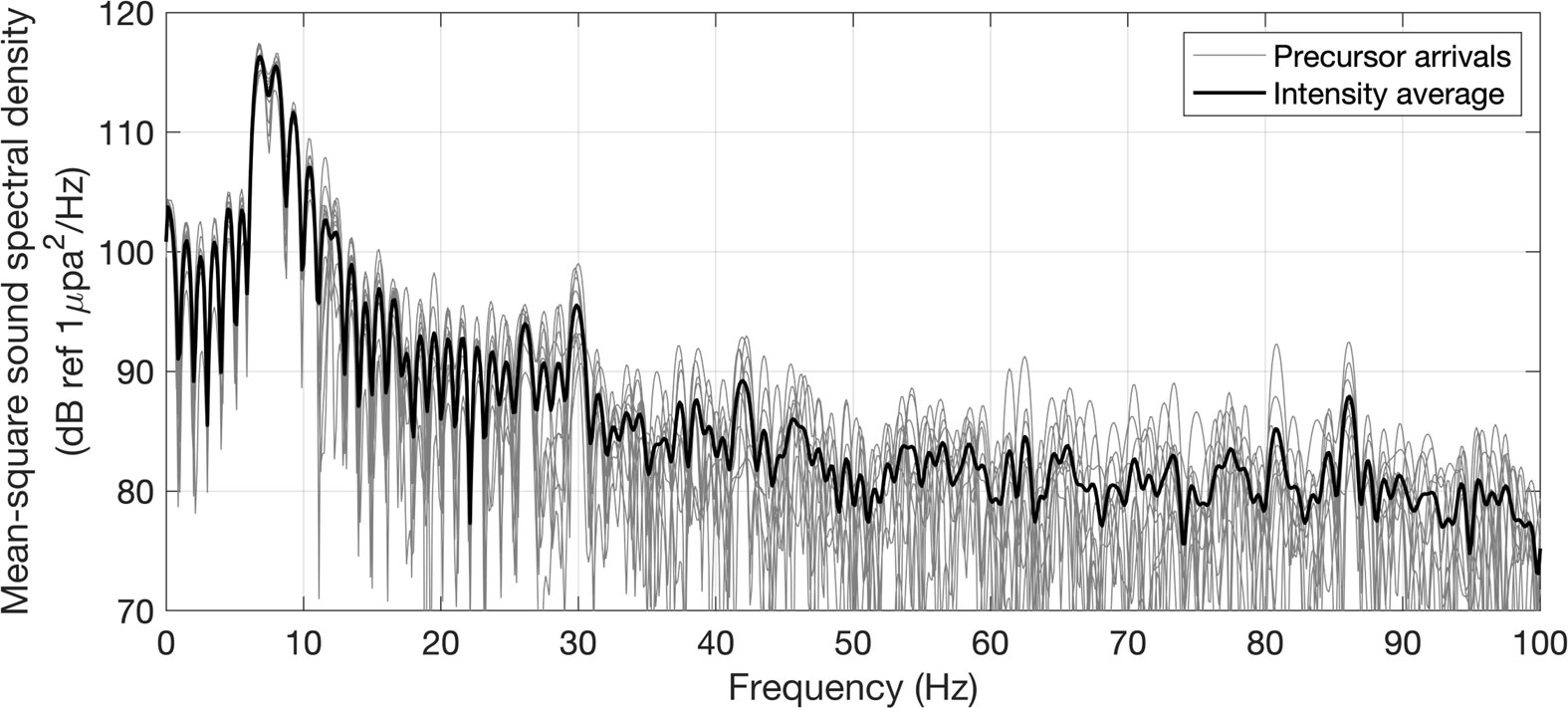
Figure 6 Mean-square sound spectral densities of precursor arrivals. The spectrum levels of 10 pulses and their intensity average are represented by thin gray lines and thick black line, respectively.

Airgun sound propagation showed a significant difference between the measurements and PE model predictions. Although the rare core data describing the sound speed and density in layer-2 were cited, they may differ from our conditions. As mentioned in Section 1, the survey region could be composed of cemented subsurface sediment and was also reported to be the permafrost distributed region (Brown et al., 1997; Romanovskii, 2004; Niessen et al., 2013; O'Regan et al., 2017). The sound speed in frozen soils, which varies with sediment type, depth, and temperature, is much higher than that applied in the PE model predictions (LeBlanc et al., 2004). The geoacoustic properties (i.e., sound speed, density, and attenuation) of different sediment types could be applied as a function of mean grain size (Ainslie, 2010), with sound speed increasing as mean grain size decreases. Therefore, the acoustic properties of layer-2 were manually varied from those corresponding to 3 ϕ to -1 ϕ to obtain values that were consistent with the PE propagation model prediction (Supplementary Figure 3). The following values of c₂ = 1,928 m/s, ρ₂ = 2.55 g/cm³ and α₂ = 0.9076 dB/λ corresponding to the acoustic properties of -1 ϕ were applied to those in layer-2 (Ainslie, 2010). The PE model prediction curve using replaced acoustic properties shown as a dashed magenta line in Figure 5 significantly improved the RMSE of 1.8 dB but lower the back-calculated SL to 195 dB compared to the theoretical prediction of 210 dB. When cutoff frequencies were predicted using the geoacoustic properties of -1 ϕ and water depth in layer-2, which was calculated by the summation of water depth and thickness in layer-1, the two modes at a receiver depth of 74 m were 7.9 and 23.6 Hz, and the source depth of 69 m corresponds to frequencies of 8.4 and 25.2 Hz. The mode-1 cutoff frequency of approximately 8 Hz in both cases was broadly similar to the measured strong spectral peak of precursor arrivals. The applied thickness of the layer-1 is linearly interpolated from 4 to 3 m. The variation in cutoff frequencies with a thickness of 1 m was less than 0.5 Hz. Figure 7 shows the predicted cutoff frequencies as a function of depth inverted on the x-axis to consider the depth variation for the source moving away from the receiver, as shown in Figure 4B. As the water depth decreases and the mode number increases, the cutoff frequency increases. The cutoff frequencies of modes 1 and 2 were less than 40 Hz, and those of mode 3 did not exceed 50 Hz up to depths above 58 m. When the depth range dependently decreased, as in our measurements, the increase in the cutoff frequency was steeper than that predicted by the mode coupling (Katsnelson et al., 2012). In addition, because the sound speed in the sediment layer is not constant with the depth, the perfect trapping mode could not occur, and the sound could propagate relatively weakly even below the predicted cutoff frequency Figure 7.

FIGURE 7

Figure 7 Cutoff frequency as a function of depth in layer-2 inverted on the x-axis. Blue, red, and black lines show the cutoff frequencies of modes 1, 2, and 3, respectively. The shaded gray area represents the vertical errors caused by the depth variation by ± 2 m.

Figure 8 shows the expanded scale of Figure 4E with predicted modal dispersion curves. Low-frequency impulsive airgun sound propagating over several kilometers is dispersive, and the received signal can be interpreted as a sum of modal components. Each mode propagates with its frequency-dependent group velocities (v_g), which can be derived from the horizontal wavenumber (k_h) and angular frequency (ω ) (Frisk, 1994; Jensen, 2011; Bonnel et al., 2020):

FIGURE 8

Figure 8 The spectrogram of a single airgun pulse, which is an expanded scale of Figure 4E. Gray and black circles represent the predicted modal dispersion curves of the three modes at 69 and 74 m, respectively (which are layer-2 depths at the source and receiver locations).

$\begin{array}{ll}{v}_g=\frac{d\omega }{d{k}_h}& (7)\end{array}$

The gray and black circles show dispersion curves predicted when acoustic properties in layer-2, a distance of 18,566 m, and source and receiver depths of 69 and 74 m were applied. The dispersion curves of modes 1 and 2 appeared clearly in the spectrogram and were closely matched with the prediction curves, whereas the curve of mode 3 was vague. This trend could correspond with the number of propagating modes of 2.6 and 2.7 calculated in Equation 6.

Propagation characteristics of airgun sound may vary depending on the airgun type, operating scheme, and environmental variability of the ocean. Although we predicted the transmission losses using the regression curve with variables of the spreading constant and attenuation coefficient, Thode et al. (2010) investigated airgun sound propagation under cylindrical spreading with a single variable of attenuation depending on the presence or absence of sea ice cover. The attenuation coefficient may differ because their measurements were conducted in a deeper water and at farther distances than ours, and the airgun type was different. RAM was used in the present study to investigate low-frequency dominant airgun sound and range-dependent bottom properties. In addition, other numerical models based on the normal mode or wavenumber integration theorem may be used. Duncan et al. (2013) reported relatively low transmission losses at narrow and low frequencies related to the effect of the cemented hard rock layer with attenuation coefficient and shear wave properties at the Australian continental shelf. Although the contribution of shear wave properties was not considered in the present study, if the lower layer is consolidated enough to exhibit the effect of shear, it needs to be considered in the seabed. Furthermore, the density and attenuation coefficient of the sediment were applied based on the sound speed corresponding to the measured mean grain size, but their contribution to the sound propagation in the numerical model prediction is significant. Once the high-resolution geological data such as deep core measurements will be obtained, advanced prediction and verification may be performed. Finally, the precursor arrivals and modal dispersion discussed here were dealt with only in a short-range with a high signal-to-noise ratio, and intensive studies on their variation with distance are needed.

5 Conclusion and implications

Seismic airgun sounds were measured as a function of distance in shallow water along the East Siberian Shelf, and their acoustic characteristics in the time and frequency domains were investigated. The measured sound pressure levels in L_p, L_E, and L_B were compared with the predictions from the regression analysis with the initial amplitude scaled from the near-field hydrophone data. Range-dependent propagation of the airgun sounds were predicted by using the broadband PE model with the measured source spectrum, and those estimated from a high-velocity sedimentary layer based on the geological history of the region are in close agreement with the measured sound pressure level in L_B showing slightly greater than spherical spreading on the regression curve. The effects of the cutoff frequency, precursor arrivals and modal dispersion were observed and discussed considering the environmental conditions and geometry of acoustic measurements. Our results imply that the geoacoustic structure of the measurement area could be a glaciogenic overcompacted sedimentary layer created by the grounding events of ice masses through the repeated glacial advance and retreat or be the permafrost distributed region. Recently, studies on inversion using warping techniques have been conducted (Thode et al., 2017; Bonnel et al., 2020). Our results can be applied in the improved inversion of the geoacoustic parameters and measurement geometry as a follow-up study combined with the seismic survey data analysis of the period in progress and deep core data collection. In addition, the impact of anthropogenic noise on the ocean environment is being actively studied based on multidisciplinary research (Slabbekoorn et al., 2010; Ellison et al., 2012; Hawkins and Popper, 2014; Ainslie et al., 2016), and our results may be used for the impact assessment of airgun sound. However, it should be carefully discussed; thus we focused on the acoustic characteristics of seismic airgun sounds and their propagation. In this regard, our results can be used to recognize the variations in the underwater acoustic environment caused by seismic surveys and to develop mitigation strategies and sustainable operating plans.

Data availability statement

The original contributions presented in the study are included in the article/Supplementary Material. Further inquiries can be directed to the corresponding author.

Author contributions

D-GH carried out acoustic data analysis and propagation modeling. HL conceptualized this research. SK, YC and YJ designed and conducted the MCS survey. ML predicted the near-field signature and its amplitude. WS designed the autonomous hydrophone mooring. DL and YY performed predictions of modal dispersion. HL, JC, EY, JH, S-HK, TR, and HS contributed to the supervision and validation of the measurement and prediction results. All authors contributed to writing the original draft and editing the manuscript. All authors contributed to the article and approved the submitted version.

Funding

This research was supported by Korea Institute of Marine Science & Technology Promotion (KIMST) funded by the Ministry of Oceans and Fisheries (20210605, Korea-Arctic Ocean Warming and Response of Ecosystem, KOPRI and 20210632, Survey of Geology and Seabed Environmental Change in the Arctic Seas, KOPRI).

Conflict of interest

The authors declare that the research was conducted in the absence of any commercial or financial relationships that could be construed as a potential conflict of interest.

Publisher’s note

All claims expressed in this article are solely those of the authors and do not necessarily represent those of their affiliated organizations, or those of the publisher, the editors and the reviewers. Any product that may be evaluated in this article, or claim that may be made by its manufacturer, is not guaranteed or endorsed by the publisher.

Supplementary material

The Supplementary Material for this article can be found online at: https://www.frontiersin.org/articles/10.3389/fmars.2023.956323/full#supplementary-material

References

Abadi S. H., Freneau E. (2019). Short-range propagation characteristics of airgun pulses during marine seismic reflection surveys. J. Acoust Soc. Am. 146, 2430. doi: 10.1121/1.5127843

PubMed Abstract | CrossRef Full Text | Google Scholar

Ainslie M. (2010). Principles of sonar performance modelling (Berlin, Heidelberg: Springer Berlin Heidelberg : Imprint: Springer).

Google Scholar

Ainslie M. A., Halvorsen M. B., Dekeling R. P. A., Laws R. M., Duncan A. J., Frankel A. S., et al. (2016). “Verification of airgun sound field models for environmental impact assessment”. In Proceedings of Meetings on Acoustics, 27(1), p. 070018. Acoustical Society of America. doi: 10.1121/2.0000339

CrossRef Full Text | Google Scholar

Ainslie M. A., Laws R. M., Sertlek H. O. (2019). International airgun modeling workshop: Validation of source signature and sound propagation models–Dublin (Ireland), July 16, 2016–problem description. IEEE J. Oceanic Eng. 44, 565–574. doi: 10.1109/joe.2019.2916956

CrossRef Full Text | Google Scholar

Alexander O. (2000). An acoustic modeling study of seismic air gun noise in queen Charlotte basin (Canada: University of Victoria).

Google Scholar

Bonnel J., Thode A., Wright D., Chapman R. (2020). Nonlinear time-warping made simple: A step-by-step tutorial on underwater acoustic modal separation with a single hydrophone. J. Acoust Soc. Am. 147, 1897. doi: 10.1121/10.0000937

PubMed Abstract | CrossRef Full Text | Google Scholar

Brown J., Ferrians Jr. O. J., Heginbottom J. A., Melnikov E. S. (1997). Circum-arctic map of permafrost and ground ice conditions. (Washington, D. C.: U. S. Geological Survey). Available: https://web.archive.org/web/20170226114554id_/https://pubs.usgs.gov/cp/45/report.pdf.

Google Scholar

Caldwell J., Dragoset W. (2000). A brief overview of seismic air-gun arrays. Leading Edge 19, 898–902. doi: 10.1190/1.1438744

CrossRef Full Text | Google Scholar

Choi J. W., Dahl P. H. (2006). First-order and zeroth-order head waves, their sequence, and implications for geoacoustic inversion. J. Acoustical Soc. America 119, 3660–3668. doi: 10.1121/1.2195110

CrossRef Full Text | Google Scholar

Collins M. D. (1993). A split-step pade solution for the parabolic equation method. J. Acoustical Soc. America 93, 1736–1742. doi: 10.1121/1.406739

CrossRef Full Text | Google Scholar

Dahl P. H., Dall'Osto D. R. (2017). On the underwater sound field from impact pile driving: Arrival structure, precursor arrivals, and energy streamlines. J. Acoust Soc. Am. 142 (2),1141–1155. doi: 10.1121/1.4999060

PubMed Abstract | CrossRef Full Text | Google Scholar

De Robertis A., Wilson C. (2011). “Underwater radiated noise measurements of a noise-reduced research vessel: comparison between a US navy noise range and a simple hydrophone mooring”. In Proceedings of Meetings on Acoustics. 12 (1), p. 070003. Acoustical Society of America. doi: 10.1121/1.3660550

CrossRef Full Text | Google Scholar

Dove D., Polyak L., Coakley B. (2014). Widespread, multi-source glacial erosion on the chukchi margin, Arctic ocean. Quaternary Sci. Rev. 92, 112–122. doi: 10.1016/j.quascirev.2013.07.016

CrossRef Full Text | Google Scholar

Dragoset W. H. (1990). Air-gun array specs: A tutorial. Leading Edge 9, 24–32. doi: 10.1190/1.1439671

CrossRef Full Text | Google Scholar

Dragoset B. (2000). Introduction to air guns and air-gun arrays. Leading Edge 19, 892–897. doi: 10.1190/1.1438741

CrossRef Full Text | Google Scholar

Duncan A. J., Gavrilov A. N. (2019). The CMST airgun array model–a simple approach to modeling the underwater sound output from seismic airgun arrays. IEEE J. Oceanic Eng. 44, 589–597. doi: 10.1109/joe.2019.2899134

CrossRef Full Text | Google Scholar

Duncan A. J., Gavrilov A. N., Mccauley R. D., Parnum I. M., Collis J. M. (2013). Characteristics of sound propagation in shallow water over an elastic seabed with a thin cap-rock layer. J. Acoust Soc. Am. 134, 207–215. doi: 10.1121/1.4809723

PubMed Abstract | CrossRef Full Text | Google Scholar

Duncan A. J., Weilgart L. S., Leaper R., Jasny M., Livermore S. (2017). A modelling comparison between received sound levels produced by a marine vibroseis array and those from an airgun array for some typical seismic survey scenarios. Mar. pollut. Bull. 119, 277–288. doi: 10.1016/j.marpolbul.2017.04.001

PubMed Abstract | CrossRef Full Text | Google Scholar

Ellison W. T., Southall B. L., Clark C. W., Frankel A. S. (2012). A new context-based approach to assess marine mammal behavioral responses to anthropogenic sounds. Conserv. Biol. 26, 21–28. doi: 10.1111/j.1523-1739.2011.01803.x

PubMed Abstract | CrossRef Full Text | Google Scholar

Frisk G. V. (1994). Ocean and seabed acoustics : a theory of wave propagation (Englewood Cliffs, N.J: PTR Prentice Hall).

Google Scholar

Gisiner R. C. (2016). Sound and marine seismic surveys. Acoust. Today 12, 10–18. Available: https://acousticstoday.org/wp-content/uploads/2016/12/Seismic-Surveys.pdf.

Google Scholar

Han D. G., Choi J. W. (2022). Measurements and spatial distribution simulation of impact pile driving underwater noise generated during the construction of offshore wind power plant off the southwest coast of Korea. Front. Mar. Sci. 8. doi: 10.3389/fmars.2021.654991

CrossRef Full Text | Google Scholar

Han D.-G., Joo J., Son W., Cho K. H., Choi J. W., Yang E. J., et al. (2021). Effects of geophony and anthrophony on the underwater acoustic environment in the East Siberian Sea, Arctic ocean. Geophysical Res. Lett. 48 (12), e2021GL093097. doi: 10.1029/2021gl093097

CrossRef Full Text | Google Scholar

Hawkins A. D., Popper A. N. (2014). Assessing the impacts of underwater sounds on fishes and other forms of marine life. Acoustics Today 10, 30–41. Available: https://acousticstoday.org/wp-content/uploads/2015/05/Assessing-the-Impact-of-Underwater-Sounds-on-Fishes-and-Other-Forms-of-Marine-Life-Anthony-D.-Hawkins-and-Arthur-N.-Popper.pdf.

Google Scholar

Hawkins A. D., Popper A. N. (2017). A sound approach to assessing the impact of underwater noise on marine fishes and invertebrates. ICES J. Mar. Sci. 74 (3), 635–651. doi: 10.1093/icesjms/fsw205

CrossRef Full Text | Google Scholar

Heaney K. D., Campbell R. L. (2019). Parabolic equation modeling of a seismic airgun array. IEEE J. Oceanic Eng. 44, 621–632. doi: 10.1109/joe.2019.2912060

CrossRef Full Text | Google Scholar

Hegewald A., Jokat W. (2013). Relative sea level variations in the chukchi region-Arctic ocean-since the late Eocene. Geophysical Res. Lett. 40, 803–807. doi: 10.1002/grl.50182

CrossRef Full Text | Google Scholar

Hermannsen L., Tougaard J., Beedholm K., Nabe-Nielsen J., Madsen P. T. (2015). Characteristics and propagation of airgun pulses in shallow water with implications for effects on small marine mammals. PloS One 10, e0133436. doi: 10.1371/journal.pone.0133436

PubMed Abstract | CrossRef Full Text | Google Scholar

Hovem J. M., Tronstad T. V., Karlsen H. E., Lokkeborg S. (2012). Modeling propagation of seismic airgun sounds and the effects on fish behavior. IEEE J. Oceanic Eng. 37, 576–588. doi: 10.1109/joe.2012.2206189

CrossRef Full Text | Google Scholar

ISO 18405 (2017). Underwater Acoustics – Terminology: 2017 (Geneva: International Standardization Organization). Available: https://www.iso.org/standard/62406.html.

Google Scholar

Jensen F. B. (2011). Computational ocean acoustics (New York: Springer).

Google Scholar

Jin Y. K. (2020) ARA10C cruise report: Korea- Russia East Siberian/Chukchi Sea research program. Available at: http://library.kopri.re.kr/search/detail/CATTOT000000055761.

Google Scholar

Katsnelson B., Petnikov V., Lynch J. (2012). Fundamentals of shallow water acoustics (New York: Springer).

Google Scholar

Kavanagh A. S., Nykanen M., Hunt W., Richardson N., Jessopp M. J. (2019). Seismic surveys reduce cetacean sightings across a large marine ecosystem. Sci. Rep. 9, 19164. doi: 10.1038/s41598-019-55500-4

PubMed Abstract | CrossRef Full Text | Google Scholar

Keen K. A., Thayre B. J., Hildebrand J. A., Wiggins S. M. (2018). Seismic airgun sound propagation in Arctic ocean waveguides. Deep Sea Res. Part I: Oceanographic Res. Papers 141, 24–32. doi: 10.1016/j.dsr.2018.09.003

CrossRef Full Text | Google Scholar

Kim S., Polyak L., Joe Y. J., Niessen F., Kim H. J., Choi Y., et al. (2021). Seismostratigraphic and geomorphic evidence for the glacial history of the northwestern chukchi margin, Arctic ocean. J. Geophysical Research: Earth Surface 126 (4), e2020JF006030. doi: 10.1029/2020jf006030

CrossRef Full Text | Google Scholar

Kinsler L. E. (2000). Fundamentals of acoustics (New York: Wiley).

Google Scholar

Koessler M. W., Duncan A. J., Gavrilov A. N. (2017). Low-frequency acoustic propagation modelling for Australian range-independent environments. Acoustics Aust. 45, 331–341. doi: 10.1007/s40857-017-0108-5

CrossRef Full Text | Google Scholar

Krail P. M. (2010). Airguns: Theory and operation of the marine seismic source. Course notes for GEO-391: Principles of seismic data acquisition. (Austin: University of Texas at Austin), 1–44. Available: http://hdl.handle.net/2152/11226.

Google Scholar

Landrø M. (1992). MODELLING OF GI GUN SIGNATURES1. Geophysical Prospecting 40, 721–747. doi: 10.1111/j.1365-2478.1992.tb00549.x

CrossRef Full Text | Google Scholar

Landrø M., Amundsen L. (2018). Introduction to exploration geophysics with recent advances. (Riga, Latvia: Bivrost). Available: https://www.researchgate.net/publication/325107897_Introduction_to_Exploration_Geophysics_with_Recent_Advances.

Google Scholar

Landrø M., Hatchell P. (2012). Normal modes in seismic data–revisited. Geophysics 77, W27–W40. doi: 10.1190/geo2011-0094.1

CrossRef Full Text | Google Scholar

Landrø M., Strandenes S., Vaage S. (1991). Use of near-field measurements to compute far-field marine source signatures-evaluation of the method. First break 9 (8). doi: 10.3997/1365-2397.1991018

CrossRef Full Text | Google Scholar

Laws R., Landrø M., Amundsen L. (1998). An experimental comparison of three direct methods of marine source signature estimation. Geophysical prospecting 46, 353–389. doi: 10.1046/j.1365-2478.1998.980334.x

CrossRef Full Text | Google Scholar

LeBlanc A.-M., Fortier R., Allard M., Cosma C., Buteau S. (2004). Seismic cone penetration test and seismic tomography in permafrost. Can. Geotechnical J. 41, 796–813. doi: 10.1139/t04-026

CrossRef Full Text | Google Scholar

Marine Traffic (2019) AIS data of IBRV ARAON from 2019-09-09 to 2019-09-10. Available at: http://marinetraffic.com.

Google Scholar

Martin S. B., Matthews M. R., Macdonnell J. T., Broker K. (2017). Characteristics of seismic survey pulses and the ambient soundscape in Baffin bay and Melville bay, West Greenland. J. Acoust Soc. Am. 142, 3331. doi: 10.1121/1.5014049

PubMed Abstract | CrossRef Full Text | Google Scholar

Niessen F., Hong J. K., Hegewald A., Matthiessen J., Stein R., Kim H., et al. (2013). Repeated pleistocene glaciation of the East Siberian continental margin. Nat. Geosci. 6, 842–846. doi: 10.1038/ngeo1904

CrossRef Full Text | Google Scholar

O'Regan M., Backman J., Barrientos N., Cronin T. M., Gemery L., Kirchner N., et al. (2017). The de long trough: a newly discovered glacial trough on the East Siberian continental margin. Climate Past 13, 1269–1284. doi: 10.5194/cp-13-1269-2017

CrossRef Full Text | Google Scholar

Pascouet A. (1991). Something new under the water: The bubbleless air gun. Leading Edge 10, 79–81. doi: 10.1190/1.1436793

CrossRef Full Text | Google Scholar

Prior M. K., Ainslie M. A., Halvorsen M. B., Hartstra I., Laws R. M., MacGillivray A., et al. (2021). Characterization of the acoustic output of single marine-seismic airguns and clusters: The svein vaage dataset. J. Acoustical Soc. America 150 (5), 3675–3692. doi: 10.1121/10.0006751

CrossRef Full Text | Google Scholar

Romanovskii N. (2004). Permafrost of the east Siberian Arctic shelf and coastal lowlands. Quaternary Sci. Rev. 23, 1359–1369. doi: 10.1016/j.quascirev.2003.12.014

CrossRef Full Text | Google Scholar

Slabbekoorn H., Bouton N., Van Opzeeland I., Coers A., Ten Cate C., Popper A. N. (2010). A noisy spring: the impact of globally rising underwater sound levels on fish. Trends Ecol. Evol. 25, 419–427. doi: 10.1016/j.tree.2010.04.005

PubMed Abstract | CrossRef Full Text | Google Scholar

Thode A., Bonnel J., Thieury M., Fagan A., Verlinden C., Wright D., et al. (2017). Using nonlinear time warping to estimate north pacific right whale calling depths in the Bering Sea. J. Acoustical Soc. America 141, 3059–3069. doi: 10.1121/1.4982200

CrossRef Full Text | Google Scholar

Thode A., Kim K. H., Greene C. R. Jr., Roth E. (2010). Long range transmission loss of broadband seismic pulses in the Arctic under ice-free conditions. J. Acoust Soc. Am. 128, EL181–EL187. doi: 10.1121/1.3479686

PubMed Abstract | CrossRef Full Text | Google Scholar

van der Schaar M., Haugerud A. J., Weissenberger J., De Vreese S., André M. (2017). Arctic Anthropogenic sound contributions from seismic surveys during summer 2013. Front. Mar. Sci. 4. doi: 10.3389/fmars.2017.00175

CrossRef Full Text | Google Scholar

Ziolkowski A. (1970). A method for calculating the output pressure waveform from an air gun. Geophysical J. Int. 21, 137–161. doi: 10.1111/j.1365-246X.1970.tb01773.x

CrossRef Full Text | Google Scholar

Ziolkowski A., Parkes G., Hatton L., Haugland T. (1982). The signature of an air gun array: Computation from near-field measurements including interactions. Geophysics 47, 1413–1421. doi: 10.1190/1.1441289

CrossRef Full Text | Google Scholar