Stability prediction of muddy submarine channel slope based on sub-bottom profile acoustic images and transfer learning

This research addresses the challenging task of predicting the stability of muddy submarine channel slopes, crucial for ensuring safe port operations. Traditional methods falter due to the submerged nature of these channels, impacting navigation and infrastructure maintenance. The proposed approach integrates sub-bottom profile acoustic images and transfer learning to predict slope stability in Lianyungang Port. The study classifies slope stability into four categories: stable, creep, expansion, and unstable based on oscillation amplitude and sound intensity. Utilizing a sub-bottom profiler, acoustic imagery is collected, which is then enhanced through Gabor filtering. This process generates source data to pre-train Visual Geometry Group (VGG)16 neural network. This research further refines the model using targeted data, achieving a 97.92% prediction accuracy. When benchmarked against other models and methods, including VGG19, Inception-v3, Densenet201, Decision Tree (DT), Naive Bayes (NB), Support Vector Machine (SVM), and an unmodified VGG16, this approach exhibits superior accuracy. This model proves highly effective for real-time analysis of submarine channel slope dynamics, offering a significant advancement in marine safety and operational efficiency.

1 Introduction

The morphology of submarine channel slopes, often manually excavated, is influenced by various factors such as storm surges, waves, sediment deposition, and ship traffic (Wang et al., 2014; Lawson et al., 2021). Extended creep in these slopes can lead to instability, reshaping the channel and impeding safe navigation, which negatively impacts port economic development (Sultan et al., 2004; Hojat et al., 2019). Consequently, predicting the stability of these submarine channel slopes is crucial.

Advancements in computer vision and artificial intelligence, especially deep learning and transfer learning, have greatly enhanced the assessment and prediction of slope stability. These technologies are widely applied in fields like target detection (Zhang et al., 2019; Xu et al., 2022a), evaluation (Fu et al., 2023; Wang et al., 2023), prediction (Long et al., 2022; Zhang and Zhang, 2022), and classification (Chungath et al., 2022; Zhang et al., 2022). Yang and Mei (2021) effectively used transfer learning for surface crack detection on slopes. Similarly, Qin et al. (2022) applied transfer learning for landslide detection using satellite images. Liu et al. (2021) combined transfer learning with limited remote sensing images for landslide type prediction in the southeast Tibetan Plateau. These studies validate the effectiveness of transfer learning in forecasting geological disasters, providing rapid and efficient monitoring and early warning capabilities for slope stability.

Existing research on slope hazards primarily focuses on surface slopes, where data collection is relatively straightforward. In contrast, investigating the stability of muddy submarine channels is more challenging due to difficulties in data acquisition and the limited availability of prior research. These submarine slopes change slowly and have sediments characterized by high water content, low shear strength, and significant deformability (Vanneste et al., 2014; Manuel et al., 2022), rendering traditional methods like precision levels (Tryggvason, 1968), infrared rangefinders (Farzad et al., 2023), and side-scan sonars (Johnson and Helferty, 1990) ineffective. The advancement of sub-bottom profiling, known for its rapid propagation and strong penetration in solids and liquids (Urlaub and Villinger, 2019; Zhang, 2022), offers a solution.

This study addresses the challenges in detecting slope stability within submarine channels, utilizing a sub-bottom profiler for comprehensive walkover detection. The method constructs a prediction model for the stability of muddy submarine channel by capturing sound print image of channel slope and combining transfer learning. To enhance the accuracy of this model, a Gabor filter is employed to process the acquired sound print images, yielding amplitude and phase images. This process is augmented by supervised data enhancement techniques, creating an enriched dataset for the preliminary training of VGG16 model. This step is crucial for improving the model’s generalizability and robustness in subsequent transfer learning phases. Furthermore, the study conducts a comparative analysis of VGG16 model’s predictive capabilities post-transfer learning against other models trained via similar transfer and machine learning methodologies, under identical pre-training and environmental setups. The findings indicate superior predictive performance of VGG16 model post-transfer learning. This advancement not only bridges a gap in the domain of muddy submarine channel slope stability prediction but also significantly contributes to the safety and economic development of submarine channels. The methodologies and techniques deployed in this research have broader applications, extending their utility to related engineering and environmental contexts. The structure of the paper is methodically organized, with Section 2 detailing the data detection process and methodologies employed, Section 3 presenting criteria for data classification, experimental outcomes, and comparative model analyses, and Section 4 concluding with discussions on the study’s findings, limitations, and avenues for future research.

2 Materials and methods

2.1 Field detection

The survey was conducted in a specific area of Lianyungang Port, Jiangsu Province, situated at coordinates 34°44’-34°46’ N and 119°26’-119°32’ E (Figure 1). The area, a typical muddy shoal deep water channel, is bordered by Liandao Island to the north and Yuntai Mountain to the south.

Figure 1

Figure 1 Survey region.

For the navigation detection within this survey area (Figure 2), a SES-2000 parametric array sub-bottom profiler was deployed. The device’s transducer was affixed to a bracket on the ship, positioned at 1/3 from the bow along the waterline, with a draft depth of about 1.4 m. A Global Positioning System (GPS) was set up on a rod, maintaining a 1.5 m horizontal distance from the transducer. The system operated with a sampling frequency of 96 kHz and a period of 1 second. The gathered acoustic signals were processed using SES-2000’s ISE post-processing software, which generated sound print images characterized by different textural features like dots, lines, and blocks.

Figure 2

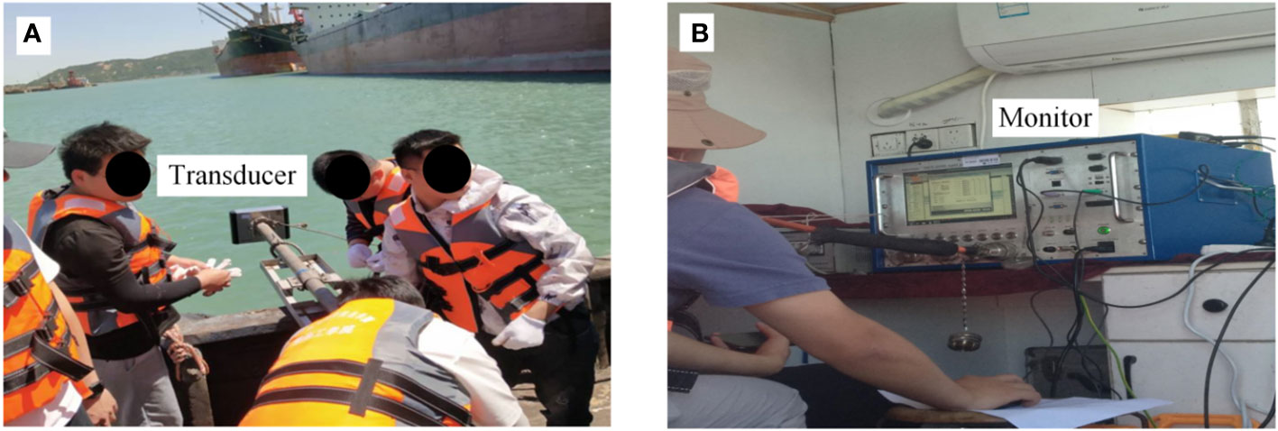
Figure 2 Field detection: (A) transducer (B) monitor.

2.2 Data processing

The study involved standardizing sound print images to a uniform size (227×227 pixels) for model compatibility, using image processing software to crop them (Figures 3A–D). A total of 400 images were manually labeled, with an equal distribution (100) across each stability state. Data enhancement was crucial to prevent overfitting, increase data volume, and enhance the model’s generalization and robustness, especially under limited data conditions. Two data enhancement approaches are recognized: supervised and unsupervised. Supervised enhancement, including techniques like noising, filtering, mirroring, rotation, and displacement (McArthur et al., 2018; Edgar et al., 2021; Neupane et al., 2021), is aimed at improving prediction and classification accuracy. On the other hand, unsupervised enhancement, such as Autoaugmentation (GAN) (Naghizadeh et al., 2021; Panetta et al., 2021), focuses on uncovering data’s inherent structures for more effective processing. This research utilized horizontal mirroring, linear transformation, Gaussian filtering, salt and pepper noise, and horizontal displacement to refine the sound print images (Figures 3E–H). This process expanded the dataset to six times its original size, yielding 2,400 images. These images served as the target data for the transfer learning model, with 70% allocated for training and 30% for testing.

Figure 3

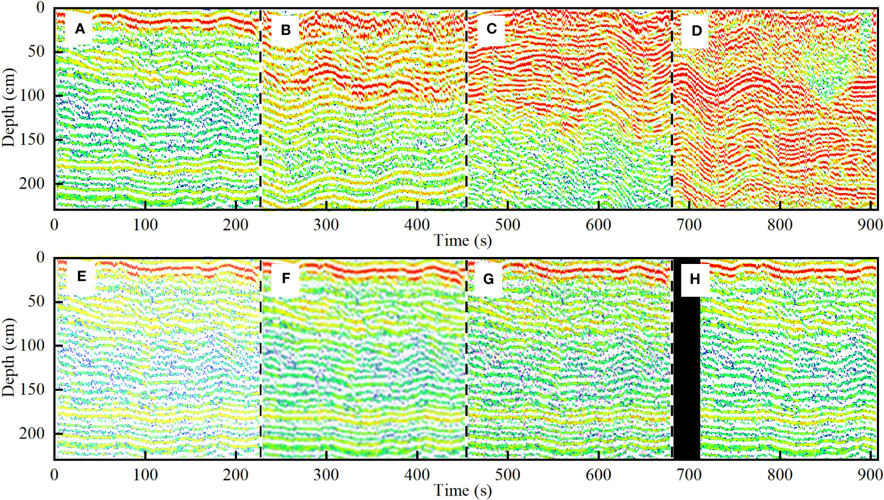
Figure 3 Target data: Sound print image (A–D) (A) stable state (B) creep state (C) expansion state (D) unstable state; Sound print enhanced image (E–H) (E) linear transformation (F) Gaussian filtering (G) salt and pepper noise (H) horizontal displacement.

2.3 Gabor filter

Gabor filter, a critical tool in texture analysis (Daugman, 1985; Idrissa and Acheroy, 2002; Rabah et al., 2022), operates as a linear filter emulating the frequency and orientation sensitivity of human vision. It is adept at detecting image edges and extracting features pertaining to specific directions and scales, with a degree of tolerance for image rotation and deformation. The filter’s ability to maintain essential spatial and frequency domain features renders it highly suitable for model pre-training. In this study, Gabor filter was applied to process sound print images in different stability states. Various parameter combinations were experimented with, such as wavelength λ, orientation θ, phase offset ψ, bandwidth σ, and aspect ratio γ, to derive amplitude and phase feature images (Table 1). Optimal feature expression in amplitude and phase was achieved with settings of λ =8, θ = 90°, ψ = 0°, σ = 1.5, and γ = 4. Images processed under these parameters were used as the primary data for model pre-training (Figures 4A–D). Enhancements to this source data included techniques like horizontal and vertical mirroring, linear and nonlinear transformation, Gaussian filtering, salt and pepper noise, horizontal and vertical displacement, and 180° rotation (Figures 4E–H). This expanded the source data to ten times its original size, resulting in a dataset of 8,000 images, with 80% designated for training and 20% for testing.

Table 1

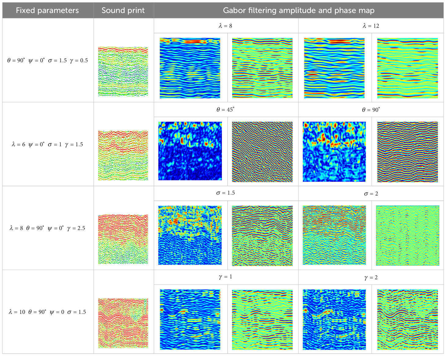
Table 1 Gabor filtering amplitude and phase map under different parameter combinations.

Figure 4

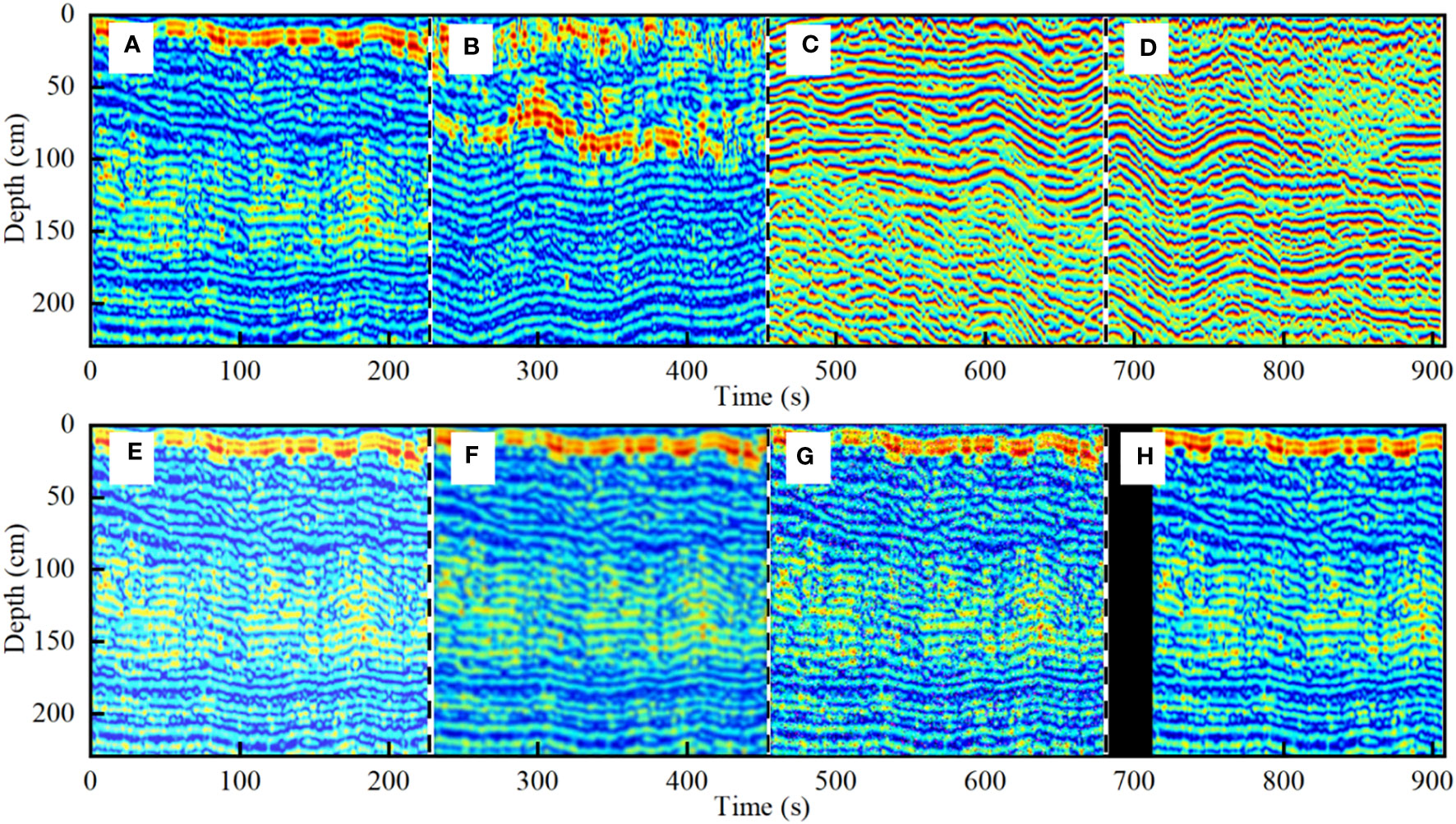
Figure 4 Source domain data: Gabor filtering image (A–D) (A, B) amplitude (C, D) phase; source domain enhanced image (E–H) (E) linear transformation (F) Gaussian filtering (G) salt and pepper noise (H) horizontal displacement.

2.4 VGG16

Visual Geometry Group (VGG) model, a deep Convolutional Neural Network (CNN) introduced in 2014, stands out for its simplicity compared to newer network structures (Tammina, 2019; Thakur et al., 2023). It uses small (3×3) convolution kernel filters in its convolutional layers, reducing parameter count, increasing network depth, and enhancing expressiveness. Rectified Linear Unit (ReLU) activation function is employed to combat gradient dissipation and increase sparsity. Unlike average pooling, maximum pooling is utilized to reduce data size while maintaining image texture, minimizing blurring effects. The training process includes a Dropout mechanism, randomly deactivating neurons to simplify the network and improve generalization. The architecture integrates fully connected layers to merge data from convolution and pooling layers into a softmax layer for classification and prediction. With its composition of 13 convolution layers, 5 pooling layers, and 3 fully connected layers, VGG16 is selected for building the transfer learning prediction model in this study due to its robust and efficient structure (Mohan et al., 2020).

2.5 Transfer learning

Transfer learning, a method of applying knowledge from one domain to similar ones, is increasingly recognized for its efficiency (Zhang et al., 2020; Iman et al., 2023). It involves transferring knowledge from a well-understood source domain to a related target domain, leveraging similarities in data, tasks, and models. This approach not only personalizes the model but also simplifies it, leading to reduced training time and enhanced learning performance in the target domain (Feldens, 2020; Zhang and Zhang, 2020). The most common technique in transfer learning is fine-tuning (Vrbančič and Podgorelec, 2020; Xu et al., 2022b), which entails using pre-trained model weights from the source domain and then adjusting these parameters with target domain data. This method offers benefits, including time efficiency and improved robustness and generalizability, especially after pre-training with large-scale data models.

This study utilized a transfer learning approach, integrating features and model structures. Experiments were conducted in the MATLAB2020 programming environment on a Windows 10 system. The process began with VGG16 model, which was pre-trained using extensive source data refined through the Gabor filter, allowing initial learning of feature information. Following this, the target data was used to fine-tune the pre-trained VGG16 model’s parameters. While the training parameters of the model’s convolutional layers, crucial for prediction and classification, remained largely unchanged, adjustments were made to the batch size and learning rate to optimize the model’s predictive accuracy. The training process of this model is depicted in Figure 5.

Figure 5

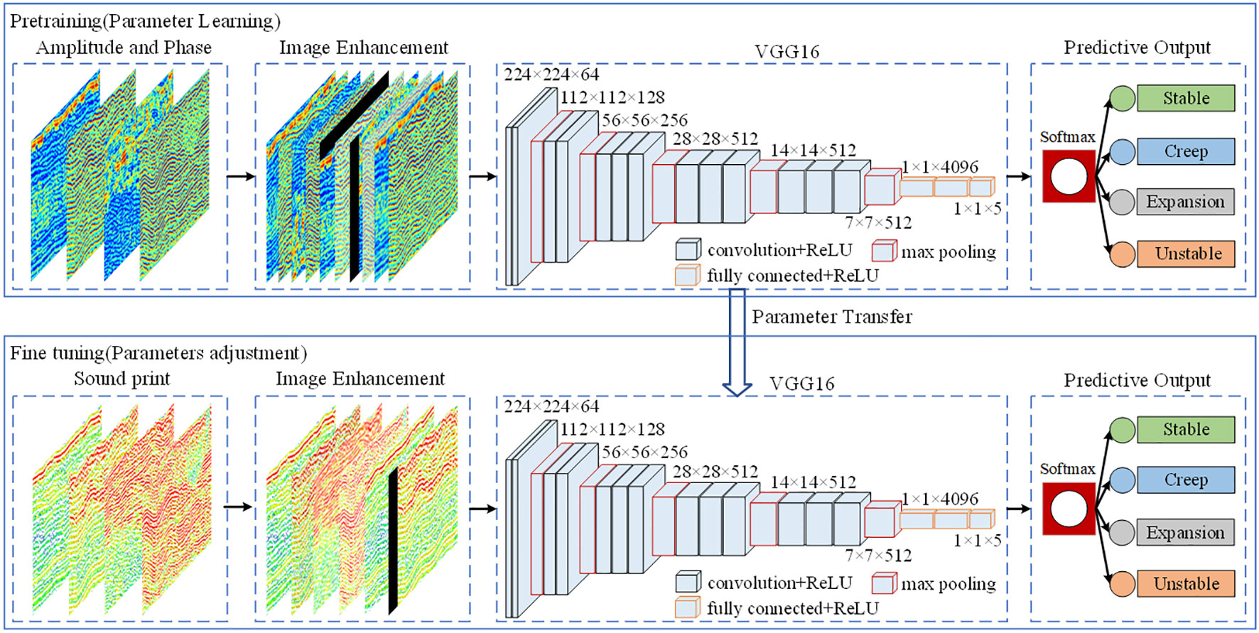
Figure 5 Flow chart of prediction model transfer learning.

Figure 6 illustrates the feature transfer process from the source domain, consisting of amplitude and phase data, to the target domain of sound print images. This model-based transfer approach hinges on identifying and utilizing shared parameters between the two domains. It operates under the assumption that certain model parameters are transferable and applicable to both source and target domain data (Gabriel and Olga, 2021). Figure 6 highlights which parameters are common and transferable across these domains. In this process, the model retains its training parameters from the source domain data, while fine-tuning is applied using the target domain data to refine and achieve the best possible prediction outcomes. The target data is integral to this fine-tuning process, playing a key role in the optimization of the model parameters.

Figure 6

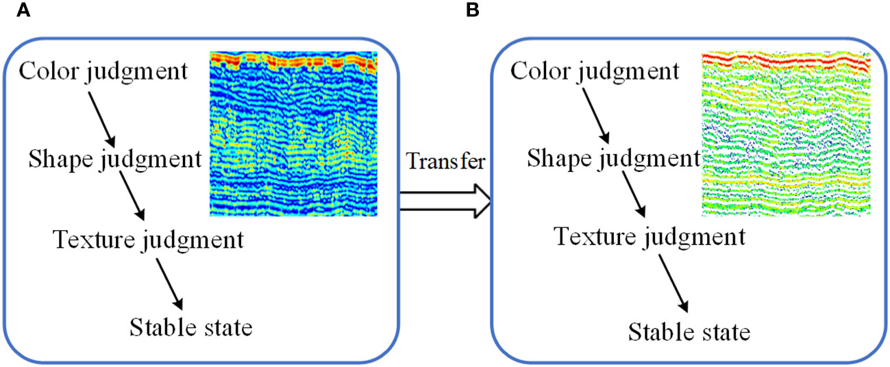
Figure 6 Schematic representation of feature transfer: (A) source domain image (B) target image.

3 Results and discussion

3.1 Channel slope state assessment

Assessing the stability of submarine channel slopes is inherently complex, owing to the interplay of multiple factors. Different times and depths in reflected signals yield varied intensity characteristics and textures in sound print images, making it difficult to accurately gauge slope stability through visual inspection alone. Sound print images, derived from sound intensity, offer a method for classifying the stability state of a channel slope. This technique provides a direct measure of the intensity and uniformity of sound print textures, thereby offering an indirect representation of the internal structure of the sediment layers. In this study, sound intensity data, extracted from the sub-bottom profiler post-processing software ISE, are utilized to determine the average sound intensity, which forms the foundation for categorizing the channel slope’s stability state. The stability is classified into four states: stable, creep, expansion, and unstable. The amplitude of sound intensity oscillation in the stable state is mostly concentrated in 1~1200 db, and the peak value of oscillation mostly appears on the surface of the slope. The amplitude of sound intensity oscillation in creep state is mostly concentrated in 1201~6000 db, and the peak value of oscillation mostly appears in the shallow layer of slope. The amplitude of sound intensity oscillation in expansion stage is mostly concentrated in 6001~12000 db, and the peak value of oscillation mostly appears in the middle layer of slope. The amplitude of sound intensity oscillation in unstable state is mostly concentrated in 12001~15000 db, and the peak value of oscillation mostly appears in the deep layer of slope. This classification is based on the oscillation amplitude and peak value variations in sound intensity, combined with insights from previous simulation experiments conducted in the region (Zhang, 2021; Zhang, 2022; Zhang and Hou, 2022).

In Figures 7A–H, the variations in sound intensity corresponding to different stability states of a channel slope are illustrated. During the stable state (Figure 7A), the sound intensity oscillation amplitude is relatively low, with the maximum average sound intensity around 1200 db. The vertical series in Figure 7E reveals a stepped decline in sound intensity, with high-frequency oscillations primarily at the slope’s surface layer. In the creep state, Figure 7B depicts an increase in the oscillation amplitude of sound intensity, reaching a maximum average of about 6000 db. The vertical series (Figure 7F) shows intensified sound intensity with high-frequency oscillation peaks in the shallow layer, coupled with distinct low-frequency oscillations. For the expansion state, Figure 7C indicates a further increase in oscillation amplitude, with the maximum average sound intensity at approximately 12000 db. The vertical series in Figure 7G demonstrates an extension of sound intensity, where the peak of high-frequency oscillation is situated in the middle layer of the slope. In the unstable state, Figure 7D displays a severe fluctuation in sound intensity oscillation amplitude, peaking at around 15000 db. The corresponding vertical series in Figure 7H shows significant changes throughout the slope, characterized by multiple peaks, with high-frequency oscillation peaks in the deeper layers. These results indicate that the oscillation amplitude and peak value of sound intensity vary markedly across different stability states. The distribution and shift in intensity can effectively indicate changes in the internal stability of the slope.

Figure 7

Figure 7 Acoustic data: Time series sound intensity (A–D) (A) stable (B) creep (C) expansion (D) unstable; Vertical series sound intensity (E–H) (E) stable (F) creep (G) expansion (H) unstable; typical sound print image (I–L) (I) stable (J) creep (K) expansion (L) unstable.

Figures 7I–L presents sound print images that qualitatively illustrate the stability states of a channel slope. In the stable state (Figure 7I), the sound print appears almost parallel, exhibiting uniform thickness and spacing, resembling a smooth, continuous curve with clearly visible surface peristalsis. For the creep state (Figure 7J), the sound print reveals peristalsis with variations in intensity, shape, and spacing. The lower part of the print changes more gradually, largely maintaining parallelism with the texture. In the expansion state (Figure 7K), the middle layer displays pronounced peristaltic sound prints with significant distortion and deformation. The texture appears rough and uneven, marked by noticeable cracks, yet it retains a roughly linear connection in local areas. During the unstable state (Figure 7L), the sound print takes on a wavy, winding pattern. The deeper layers exhibit intense peristaltic prints with irregular intensity and shape, characterized by fragmented and distorted internal textures, indicative of loss and discontinuity. These sound print images, captured by a sub-bottom profiler, provide a qualitative reflection of the internal stability of the channel slope. Therefore, they serve as a reliable data foundation for the development of a prediction model for channel slope stability using transfer learning techniques.

3.2 Feature extraction in deep CNNs

Understanding the process of feature extraction and learning in deep CNNs can be challenging. To elucidate the learning status of sound print features in VGG16 model post-transfer learning, the features of the convolution and activation layers are visualized by mapping them onto a pixel space. This visualization provides a clearer insight into the abstract nature of feature extraction and learning in CNNs. Transfer learning VGG16 model each convolution layer or activation layer has multiple channels, each channel corresponds to a feature image. For example, the 7th convolution in the model has 128 channels (128 feature images). After convolution of these channels through the first few layers, the texture of the feature image obtained by some channels is relatively obvious, and the texture features obtained by some channels almost disappear. In order to visually represent the evolution process of the model’s extraction of the four state features, this section mainly selects the feature image corresponding to a channel in the convolution layer or the activation layer for display. Figure 8 illustrates the evolution of feature extraction in the transfer learning VGG16 model.

Figure 8

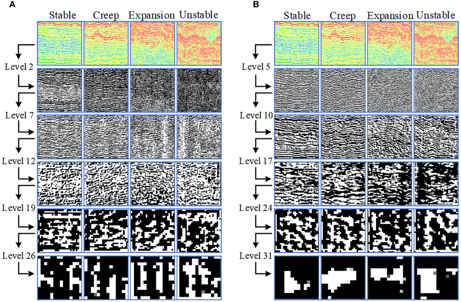
Figure 8 Evolution process of transfer learning VGG16 feature extraction: (A) convolution layer (B) activation layer.

Figure 8 illustrates the evolution of feature extraction in the transfer learning VGG16 model. Figure 8 reveals that the initial layers of the deep CNN primarily extract basic geometric features from the sound print image, such as edges, corners, and textures. These layers can also approximate the overall profile of the image. As the network progresses in depth, these elementary features are amalgamated and reorganized to form more complex, representative high-level features. Consequently, the differences of the initial image profile diminishes, and the resulting feature images become increasingly abstract.

3.3 Original model performance comparison

The performance of the original VGG16 model, chosen for this study, was evaluated by comparing it with a range of other prominent deep learning models. These included AlexNet (Schönfeldt et al., 2022), ResNet18 (Irwansyah et al., 2023), ResNet50 (Hacıefendioğlu et al., 2021), MobileNetv2 (Anupama et al., 2023), DarkNet19 (Sirisha et al., 2023), GoogleNet (Catani, 2020), and SqueezeNet (Sreeparna et al., 2022). All models were tested under identical settings, including a learning rate of 0.001, a batch size of 20, a dropout rate of 0.5, and using the Sgdm optimizer, as well as the same target data. To mitigate the issues of overfitting and underfitting during the training process, a cross-test method was employed (Bergmeir et al., 2018). In this approach, the enhanced target dataset was randomly divided five times in a 7:3 ratio, creating two subsets for each division. One subset, containing 1,680 images, was used for training, while the other, comprising 720 images, served as the test set.

Figure 9 presents the outcomes of five cross-tests involving VGG16 model and other comparative models. Figure 9A displays the prediction accuracy for each model, which is the proportion of correct predictions in the total sample size. Figure 9B shows the loss values for each model, calculated using the cross-entropy loss function to measure the deviation between predicted outputs and target values (Qu et al., 2020). The results from Figure 9 indicate that all models achieved a prediction accuracy above 80% and maintained loss values below 2.6. Notably, VGG16 model consistently exhibited the highest prediction accuracy and the lowest loss values across all training instances. For instance, in the fourth cross-test, VGG16 achieved its highest prediction accuracy at approximately 93.89% and its lowest loss value around 0.97. Conversely, the lowest prediction accuracy was observed in DarkNet19 at about 81.81%, with the highest loss value reaching approximately 2.44. These findings suggest that VGG16 is a particularly effective model for predicting the stability of channel slopes. This can be attributed to VGG16’s deeper network structure and additional convolutional layers compared to AlexNet, enhancing its ability to capture complex image features. Despite its simpler structure relative to ResNet18 and ResNet50, VGG16 demonstrates better generalization and training capabilities. Furthermore, compared to models like MobileNetv2, DarkNet19, GoogleNet, and SqueezeNet, VGG16 efficiently reduces the number of model parameters, a significant advantage when computing resources and memory are limited, thereby effectively enhancing model performance. In summary, under the specific datasets and scenarios of this study, VGG16 model outperforms its counterparts, affirming its suitability and effectiveness in this application domain.

Figure 9

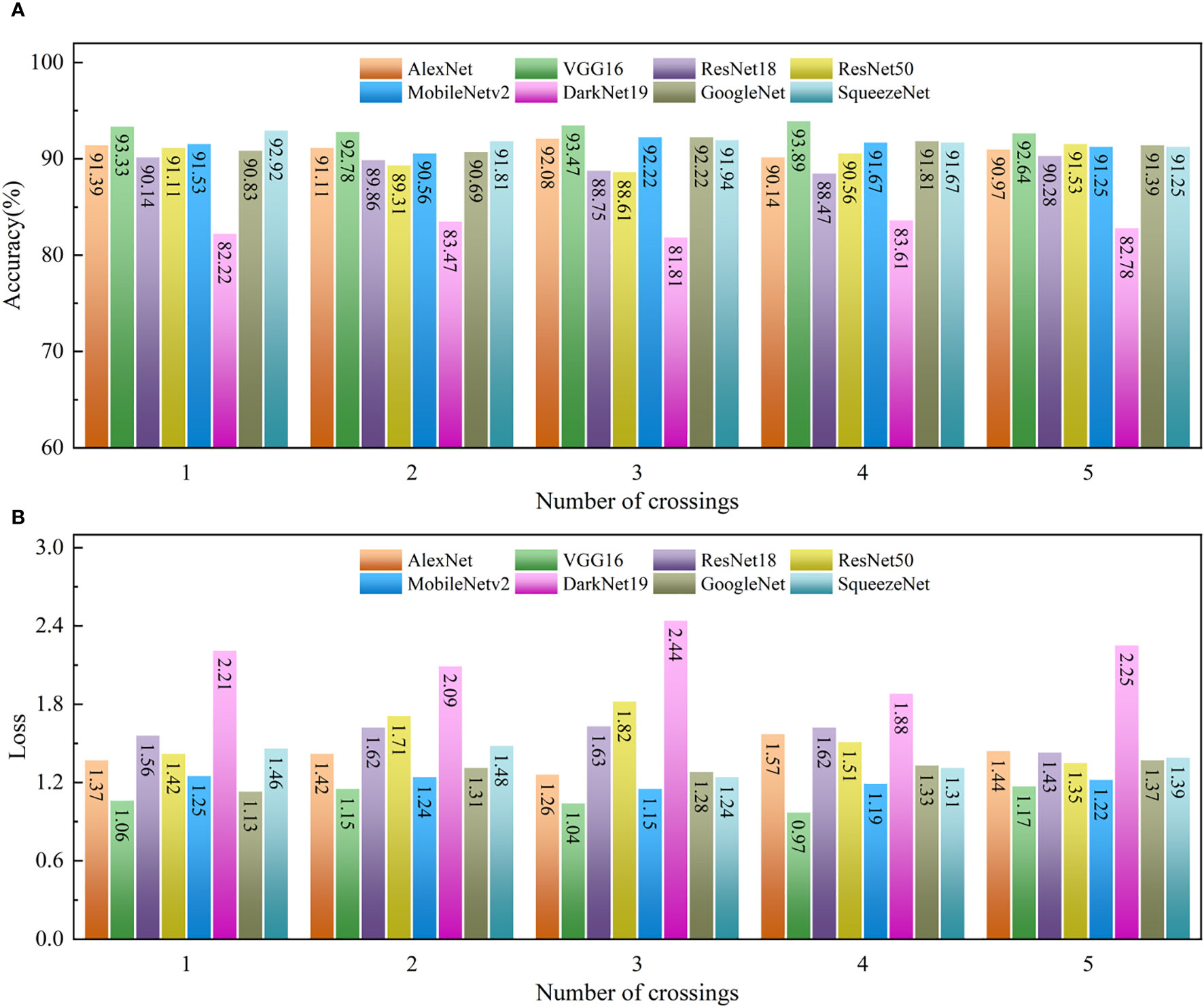
Figure 9 Results of 5 cross-tests of VGG16 and other models: (A) Accuracy (B) Loss.

Table 2 provides a comprehensive overview of the number of deep network layers in various models including VGG16, alongside their primary design purposes. AlexNet, VGG16, ResNet18, ResNet50, and DarkNet19 are predominantly developed for general object classification (Irwansyah et al., 2023; Sirisha et al., 2023). MobileNetv2 focuses on object classification in mobile and embedded devices (Chen et al., 2020), GoogleNet targets large-scale object classification (Zhuo et al., 2017), and SqueezeNet is designed for object classification in environments with embedded devices and limited computing resources (Lee et al., 2019). According to the table, MobileNetv2 possesses the highest number of deep network layers, totaling about 53. On the simpler end, AlexNet comprises 8 layers. ResNet18, DarkNet19, and SqueezeNet display a similar range in terms of their deep network layers. Additionally, Table 2 outlines the time invested in five cross-test training sessions for each model. Models like ResNet18, ResNet50, and GoogleNet required approximately 32 minutes for training. AlexNet, with fewer deep layers, took about 26 minutes. MobileNetv2 and DarkNet19, on the other hand, needed around 37 minutes.

Table 2

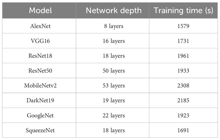
Table 2 Deep network layers for VGG16 model and other models.

3.4 Transfer model performance comparison

In this study, Gabor filter is used to process the sound print images of four states to obtain amplitude images and phase images. Each image is considered as an independent sample, and the data set is expanded by the enhancement method. Then, the amplitude image data set, phase image data set, amplitude image and phase image combined data set are divided into training set and test set according to the ratio of 8:2 to pre-train the VGG16 model. The results show that the accuracy of VGG16 model pre-trained by amplitude image is 70%, the accuracy of VGG16 model pre-trained by phase image is 65%, and the accuracy of VGG16 model pre-trained by vibration value image and phase image is 75%. This is because the amplitude image and the phase image contain different texture feature information, which has an important improvement effect on the pre-training model. Therefore, in this section, the VGG16 model pre-trained by amplitude image and phase image is selected for transfer learning.

To further improve the prediction accuracy of the transfer learning model, the enhanced original data was used to conduct experiments on the learning rate and batch size of different combinations. When the learning rate was set to 0.001 and the batch sizes were set to 20, 30, 40 and 50, the prediction accuracy of the model was 93.75%, 94.86%, 95.28% and 93.89% respectively. When the learning rate was set to 0.0001 and the batch sizes were set to 20, 30, 40 and 50, the prediction accuracy of the model was 95.56%, 95.97%, 97.92% and 95.42% respectively. When the learning rate was set to 0.00001 and the batch sizes were set to 20, 30, 40 and 50, the prediction accuracy of the model was 92.36%, 93.19%, 92.64% and 94.03% respectively. The results show that when the learning rate is set to 0.0001 and the batch size is set to 40, the prediction accuracy of the trained VGG16 model is the best. To validate the effectiveness of the proposed transfer learning VGG16 model, it was benchmarked against other network models under identical settings and data.

Figure 10 presents the comparative performance of various transfer learning models, including VGG16. All models demonstrated a prediction accuracy above 95% and a loss value below 0.6. Specifically, VGG16 model showcased the highest prediction accuracy at approximately 97.92% and the lowest loss value around 0.33. In contrast, DarkNet19 recorded the lowest prediction accuracy at roughly 95.42% and the highest loss value near 0.59. Notably, all models exhibited an improvement in accuracy by over 4% and a reduction in loss value by more than 0.6 after pre-training with source domain data prior to transfer training. This is because the Gabor filter can effectively extract the texture features and edge information in the sound print images, provide richer information to the pre-trained model, and help improve the model’s ability to understand and characterise the channel slope. At the same time, Gabor filter can help to remove the noise and irrelevant features in the sound print images, highlight the distinguishability and discrimination of the main features of the channel slope, and help the pre-trained model to extract and retain some texture features or edge information. This can effectively improve the generalization ability and robustness of the new training network model, so that the overall performance of the new model is better than the original model.

Figure 10

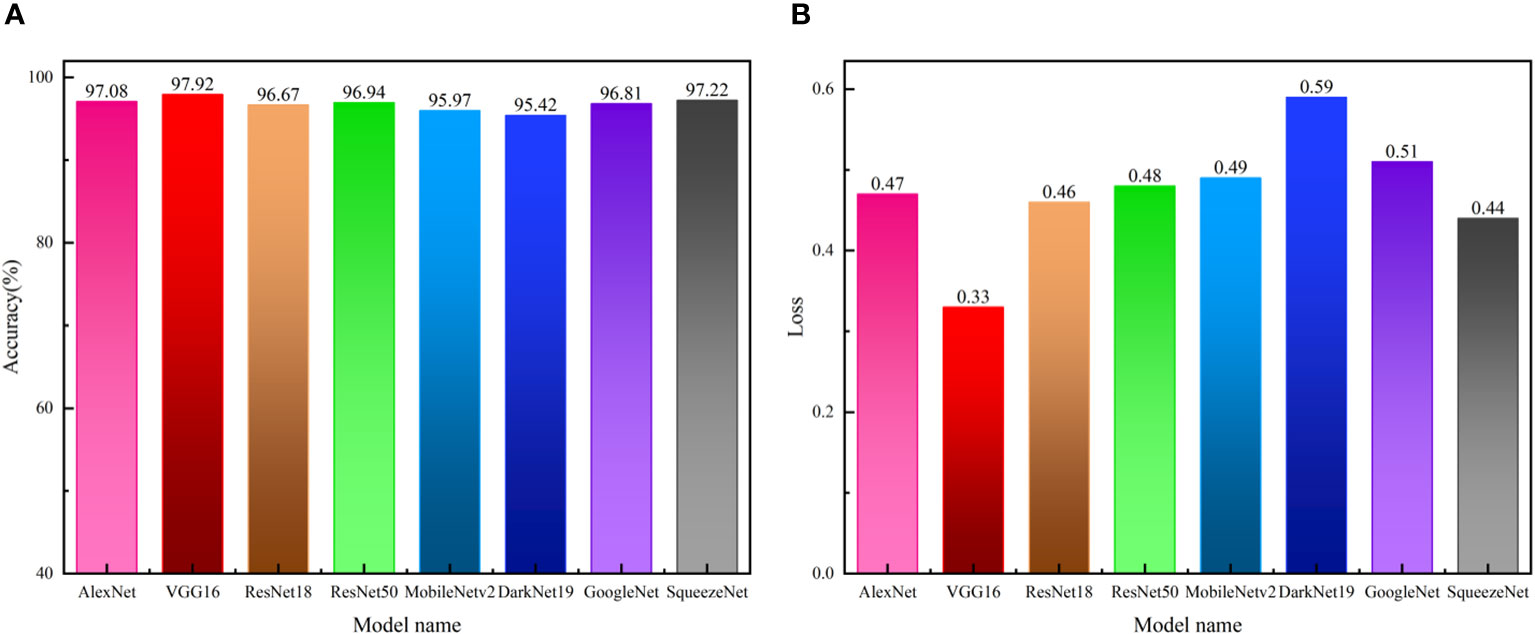
Figure 10 Performance of transfer learning VGG16 and other transfer learning models: (A) Accuracy (B) loss.

Figure 11 presents the training trajectories of both the transfer learning VGG16 model and the original VGG16 model. As training progresses through numerous iterations, an improvement in accuracy is observed for both models. However, differences emerge in their performance dynamics. The transfer learning VGG16 model, after approximately 40 iterations, shows a convergence of its accuracy and loss curves, which then proceed to run almost parallel to the horizontal axis. This indicates a quick stabilization and a steady state of performance. In contrast, the original VGG16 model, which did not undergo pre-training with source domain data, displays considerable fluctuations and more pronounced changes in its accuracy and loss curves. In terms of performance metrics, the transfer learning VGG16 model achieves a high prediction accuracy of about 97.92% and a relatively low loss value of approximately 0.33. The original VGG16 model, on the other hand, attains a prediction accuracy of around 92.64% with a loss value of about 1.17. These outcomes clearly illustrate that the transfer learning VGG16 model not only surpasses the original VGG16 in accuracy but also demonstrates greater robustness, characterized by faster convergence and quicker stabilization in its training process.

Figure 11

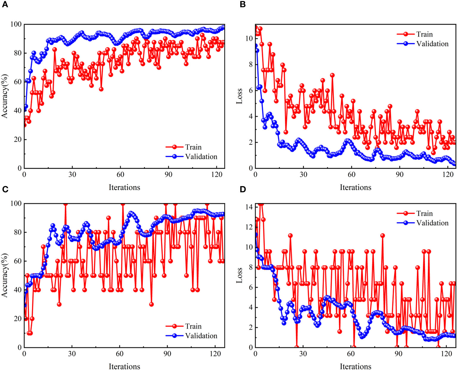
Figure 11 Model training process: Transfer learning VGG16 (A, B) (A) accuracy (B) loss; Original VGG16 (C, D) (C) accuracy (B) loss.

Figure 12 displays the test results for both the original and transfer learning VGG16 models. The data from this figure clearly demonstrate a significant improvement in the prediction accuracy of the transfer learning VGG16 model compared to the original version. Notably, the accuracy in identifying the unstable state of the channel slope has increased by up to 12.22%, with the expansion state following closely at an approximate 5% increase. The models encounter the highest error rates in accurately predicting the creep stable state and the unstable state, each with an error rate of around 3.89%. This is attributed to the ambiguity in the variation trends of sound print textures in the creep stable state, which can lead to misclassifications. In the case of the unstable state, the complexity is compounded by disturbances from seawater dynamics, where certain sound print textures might be blended or superimposed within the same image, occasionally leading to misidentification as the expansion state. Significantly, the transfer learning VGG16 model achieves a perfect 100% accuracy in predicting the stable state and a 99.44% accuracy for the expansion state. These results underscore the model’s high effectiveness and feasibility in predicting the stability of channel slopes, indicating the substantial benefits of incorporating transfer learning to enhance model performance in complex prediction scenarios.

Figure 12

Figure 12 Test set prediction results: (A) transfer learning VGG16 (B) original VGG16.

Figure 13 presents a detailed comparison of the performance metrics between the transfer learning VGG16 model and other training methodologies, including VGG19 (Liu et al., 2021), Inception-v3 (Hacıefendioğlu et al., 2021), Densenet201 (Xia et al., 2022), Decision Tree (DT) (Park et al., 2018), Naive Bayes (NB) (Zheng et al., 2021), and Support Vector Machine (SVM) (Wang and Brenning, 2021). In Figure 13A, focusing on accuracy metrics, the transfer learning VGG16 model stands out with the highest accuracy rate, approximately 97.92%. This performance markedly surpasses that of other models and methods; for instance, DT model achieves about 88.19% accuracy, and NB model around 86.95%. Figure 13B illustrates the precision rate metrics, where the transfer learning VGG16 model again leads with the highest precision rate of about 97.98%. This contrasts with slightly lower precision rates from other models, such as DT at around 88.26% and NB at approximately 86.99%. This is because VGG16 after transfer learning has a faster training speed, smaller model size and better adaptability than VGG19. Compared to Inception-v3 and Densenet201 models, VGG16 after transfer learning has a simpler architecture and number of parameters, faster training speed and better performance on limited data sets. Compared to Decision Tree (DT), Naive Bayes (NB) and Support Vector Machine (SVM), VGG16 after transfer learning can automatically extract features from the original data, automatically learn more abstract and advanced features, and has strong scalability. These findings clearly demonstrate the superiority of the transfer learning VGG16 model developed in this study, particularly in identifying the stability of muddy submarine channel slopes. Its enhanced accuracy and precision rates indicate that it is more suitable and effective for this specific application than the alternative methods compared.

Figure 13

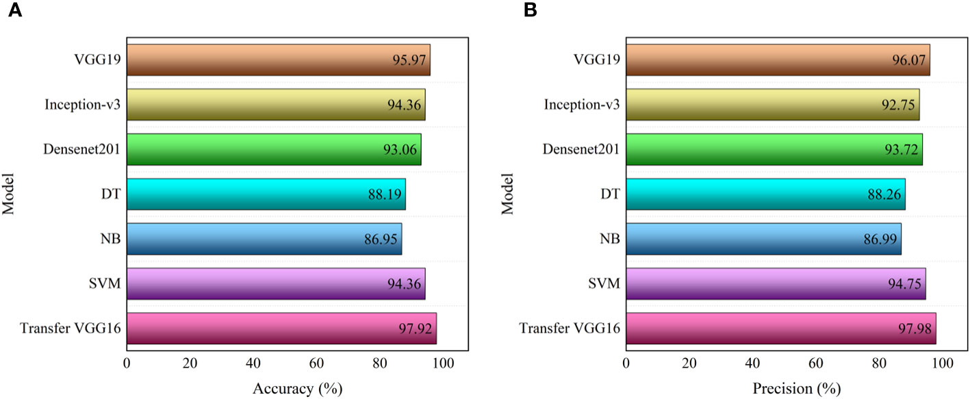
Figure 13 Transfer learning VGG16 and other method training performance metric: (A) accuracy (B) precision.

3.5 Stability prediction of channel slope

This study highlights a crucial aspect of predicting the stability of submarine channel slopes. It was observed that using the entire field detection input might overlook localized anomalous areas, which are critical for accurate stability assessment. To address this, the study employed a horizontal circulation method to segment the channel slope images from top to bottom. This segmentation approach leads to a more accurate reflection of the stability changes across the entire channel slope area. Figure 14 provides a schematic representation of the predicted slope stability for a specific muddy submarine channel located at coordinates 34°45’ 24’’-34°45’39’’N and 119°27’11’’-119°27’19’’ E (Figure 1 at position ①). Analysis of 34 sound print images from this area indicated that 30 images represented stable states, while 4 were identified as creep states. These predictions suggest that sound prints indicative of creep states are predominantly located at the shoulder or foot of the slope along the side of the channel. This pattern can be attributed to the intense seawater erosion experienced at the shoulder and the high structural self-weight at the foot of the slope. The findings imply that, overall, the submarine channel slope at this location is predominantly stable. However, localized areas, specifically the shoulder and foot of the slope, exhibit a creep state. These results are consistent with the observed development patterns of the channel slope’s stability state. The model developed in this study, therefore, proves to be of practical significance when applied to the prediction of the stability of actual muddy submarine channels, offering a valuable tool for marine and geological assessments.

Figure 14

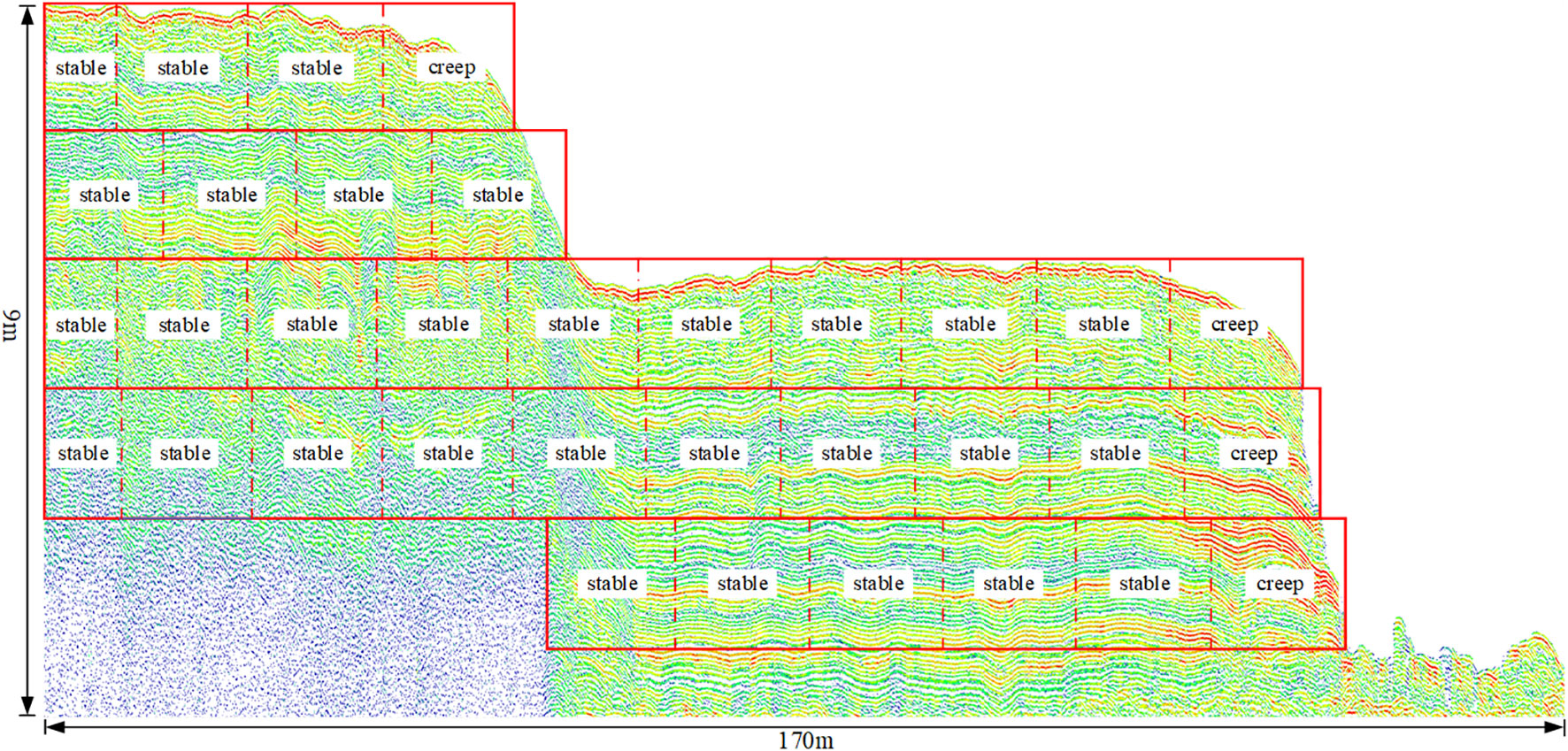
Figure 14 Schematic diagram of predicted slope results for a muddy submarine channel.

The results of this study show that the proposed model has a good predictive effect on the stability of the submarine channel slope of Lianyungang Port. In order to ensure the universality and applicability of the model to the submarine channel slope of other geographical locations, it is necessary not only to use the sub-bottom profiler to carry out navigation detection to collect sufficient data, but also to analyse and label the collected data, and to train and test the model in combination with the actual situation of the submarine channel. At the same time, considering the geological characteristics, dynamic characteristics, detection requirements and application scenarios of different geographical locations, the model needs to be further optimised to meet the prediction requirements of submarine channel slope stability in other geographical locations. In the future, we will use the sub-bottom profiler to detect the submarine channel slopes in other geographical locations, and then obtain new data samples to improve and optimise the model, so as to further enhance the applicability of the model.

4 Conclusion

This paper develops a prediction model for the stability of muddy submarine channel slopes, utilizing sub-bottom profiler sound print images and a transfer learning approach. The process involves initially classifying channel slope sound print images into four states: stable, creep, expansion, and unstable based on sound intensity variations. This classification effectively reflects slope stability in a quantitative manner. The study then employs the Gabor filter to process the images, generating amplitude and phase images, and expands these using supervised data enhancement. This expanded source data is pre-trained in VGG16 model, ensuring the preservation of spatial and frequency domain information. This pre-training enhances the model’s ability to extract and retain texture features, improving its generalization and robustness. Transfer learning is subsequently incorporated by fine-tuning the pre-trained VGG16 model with enhanced target data, including techniques like horizontal mirroring and salt and pepper noise. This fine-tuning results in a predictive model with a high accuracy of approximately 97.92% and a low loss value of approximately 0.33, outperforming other network models. This research demonstrates the feasibility of using the model for comprehensive stability prediction of channel slopes. Its significance lies in its application to port and channel safety maintenance, dynamic detection, prediction, and early warning, offering a valuable tool in marine engineering and environmental monitoring.

While the proposed method effectively predicts the stability of muddy submarine channel slopes, there are areas for improvement and innovation. One primary concern is the optimization of VGG16 network model. Given its drawbacks, such as lengthy training times, challenging parameter adjustments, and substantial storage requirements, it is not ideally suited for integration into embedded systems. Future research could explore the integration of more advanced deep network models, like Region-based CNN (RCNN) and You Only Look Once (YOLO) series, to enhance the intelligence and user-friendliness of detection outcomes. Further enhancements could be made in terms of model structure, activation functions, loss functions, and model integration, aiming to boost both performance and efficiency. Another avenue for advancement involves multi-factor coupling research. The stability of submarine channel slopes is influenced by a myriad of complex factors, including hydrodynamic forces, waves, tides, and sediment characteristics. Future studies could delve into the interrelations and coupling effects of these factors, integrating them into the predictive model for a more comprehensive analysis. Such an approach is anticipated to augment both the accuracy and reliability of model predictions.

Data availability statement

The raw data supporting the conclusions of this article will be made available by the authors, without undue reservation.

Author contributions

JH: Formal analysis, Funding acquisition, Investigation, Methodology, Software, Validation, Visualization, Writing – original draft, Writing – review & editing. CZ: Conceptualization, Data curation, Formal analysis, Funding acquisition, Project administration, Resources, Supervision, Writing – review & editing.

Funding

The author(s) declare financial support was received for the research, authorship, and/or publication of this article. The support of the Key Research and Development Program of Jiangsu Province (grant number BE2018676) and the Graduate Research and Practice Innovation Program of Jiangsu Ocean University (grant number KYCX2021-026).

Acknowledgments

The authors would like to thank Fan Y Y, Cheng W, Kong D X, Huang J G, for their help with the fieldwork experiments.

Conflict of interest

The authors declare that the research was conducted in the absence of any commercial or financial relationships that could be construed as a potential conflict of interest.

Publisher’s note

All claims expressed in this article are solely those of the authors and do not necessarily represent those of their affiliated organizations, or those of the publisher, the editors and the reviewers. Any product that may be evaluated in this article, or claim that may be made by its manufacturer, is not guaranteed or endorsed by the publisher.

References

Anupama N., Prabha S., Senthilkumar M., Sumathi R., Tag E. E. (2023). Forest fire identification in UAV imagery using X-mobileNet. Electronics 12 (3), 733–733. doi: 10.3390/ELECTRONICS12030733

CrossRef Full Text | Google Scholar

Bergmeir C., Hyndman R. J., Koo B. (2018). A note on the validity of cross-validation for evaluating autoregressive time series prediction. Comput. Stat Data Anal. 120, 70–83. doi: 10.1016/j.csda.2017.11.003

CrossRef Full Text | Google Scholar

Catani F. (2020). Landslide detection by deep learning of non-nadiral and crowdsourced optical images. Landslides 18 (2), 1–20. doi: 10.1007/s10346-020-01513-4

CrossRef Full Text | Google Scholar

Chen Y., Zheng B., Zhang Z., Wang Q., Shen C., Zhang Q. (2020). Deep learning on mobile and embedded devices: State-of-the-art, challenges, and future directions. ACM Computing Surveys (CSUR). 53 (4), 1–37. doi: 10.1145/3398209

CrossRef Full Text | Google Scholar

Chungath T. T., Nambiar A. M., Mittal A. (2022). Transfer learning and few-shot learning based deep neural network models for underwater sonar image classification with a few samples. IEEE J. Oceanic Engineering. 1–17. doi: 10.1109/JOE.2022.3221127

CrossRef Full Text | Google Scholar

Daugman J. G. (1985). Uncertainty relation for resolution in space, spatial frequency, and orientation optimized by two-dimensional visual cortical filters. JOSA A. 2 (7), 1160–1169. doi: 10.1364/josaa.2.001160

CrossRef Full Text | Google Scholar

Edgar G. M., Deysy P. G., Jesus H. M., Eduardo B. C. (2021). Multi-stage deep learning perception system for mobile robots. Integrated Computer-Aided Engineering. 28 (2), 191–205. doi: 10.3233/ICA-200640

CrossRef Full Text | Google Scholar

Farzad M., Reza M. M., Jalal K. (2023). Laboratory evaluation of infrared and ultrasonic range-finder sensors for on-the-go measurement of soil surface roughness. Soil Tillage Res. 229, 105678. doi: 10.1016/J.STILL.2023.105678

CrossRef Full Text | Google Scholar

Feldens P. (2020). Super resolution by deep learning improves boulder detection in side scan sonar backscatter mosaics. Remote Sensing. 12 (14), 2284. doi: 10.3390/rs12142284

CrossRef Full Text | Google Scholar

Fu Z., Li C., Yao W. (2023). Landslide susceptibility assessment through TrAdaBoost transfer learning models using two landslide inventories. Catena 222, 106799. doi: 10.1016/j.catena.2022.106799

CrossRef Full Text | Google Scholar

Gabriel M., Olga F. (2021). Unsupervised transfer learning for anomaly detection: Application to complementary operating condition transfer. Knowledge-Based Systems. 216, 106816. doi: 10.1016/J.KNOSYS.2021.106816

CrossRef Full Text | Google Scholar

Hacıefendioğlu K., Demir G., Başağa H. B. (2021). Landslide detection using visualization techniques for deep convolutional neural network models. Natural Hazards. 109 (1), 329–350. doi: 10.1007/s11069-021-04838-y

CrossRef Full Text | Google Scholar

Hojat A., Arosio D., Ivanov V. I., Longoni L., Papini M., Scaioni M., et al. (2019). Geoelectrical characterization and monitoring of slopes on a rainfall-triggered landslide simulator. J. Appl. Geophysics 170 (C), 103844. doi: 10.1016/j.jappgeo.2019.103844

CrossRef Full Text | Google Scholar

Idrissa M., Acheroy M. (2002). Texture classification using Gabor filters. Pattern Recognition Letters. 23 (9), 1095–1102. doi: 10.1016/S0167-8655(02)00056-9

CrossRef Full Text | Google Scholar

Iman M., Arabnia H. R., Rasheed K. (2023). A review of deep transfer learning and recent advancements. Technologies 11 (2), 40. doi: 10.3390/TECHNOLOGIES11020040

CrossRef Full Text | Google Scholar

Irwansyah E., Young H., Gunawan A. A. (2023). Multi disaster building damage assessment with deep learning using satellite imagery data. Int. J. Intell. Syst. Appl. Eng. 11 (1), 122–131. doi: 0000-0002-3876-1943

Google Scholar

Johnson H. P., Helferty M. (1990). The geological interpretation of side-scan sonar. Rev. Geophysics. 28 (4), 357–380. doi: 10.1029/RG028i004p00357

CrossRef Full Text | Google Scholar

Lawson S. K., Tanaka H., Udo K., Hiep N. T., Tinh N. X. (2021). Morphodynamics and evolution of Estuarine sandspits along the Bight of Benin coast, west Africa. Water 13 (21), 2977. doi: 10.3390/W13212977

CrossRef Full Text | Google Scholar

Lee H. J., Ullah I., Wan W., Gao Y., Fang Z. (2019). Real-time vehicle make and model recognition with the residual squeezeNet architecture. Sensors 19 (5), 982. doi: 10.3390/s19050982

PubMed Abstract | CrossRef Full Text | Google Scholar

Liu D., Li J., Fan F. (2021). Classification of landslides on the southeastern Tibet Plateau based on transfer learning and limited labelled datasets. Remote Sens. Letters. 12 (3), 286–295. doi: 10.1080/2150704X.2021.1890263

CrossRef Full Text | Google Scholar

Long J., Li C., Liu Y., Feng P., Zou Q. (2022). A multi-feature fusion transfer learning method for displacement prediction of rainfall reservoir-induced landslide with step-like deformation characteristics. Eng. Geology. 297, 106494. doi: 10.1016/j.enggeo.2021.106494

CrossRef Full Text | Google Scholar

Manuel T., António F. D. V., Diana C., Pedro T., Cristina R. (2022). Geotechnical properties of Sines Contourite Drift sediments: their contribution to submarine landslide susceptibility. Bull. Eng. Geol. Environ. 81 (9), 376. doi: 10.1007/S10064-022-02873-Y

CrossRef Full Text | Google Scholar

McArthur J., Shahbazi N., Fok R., Raghubar C., Bortoluzzi B., An A. (2018). Machine learning and BIM visualization for maintenance issue classification and enhanced data collection. Advanced Eng. Informatics. 38, 101–112. doi: 10.1016/j.aei.2018.06.007

CrossRef Full Text | Google Scholar

Mohan A., Singh A. K., Kumar B., Dwivedi R. (2020). Review on remote sensing methods for landslide detection using machine and deep learning. Trans. Emerg. Telecommun. Technol. 32 (7), e3998. doi: 10.1002/ett.3998

CrossRef Full Text | Google Scholar

Naghizadeh A., Metaxas D. N., Liu D. (2021). Greedy auto-augmentation for n-shot learning using deep neural networks. Neural Networks. 135, 68–77. doi: 10.1016/J.NEUNET.2020.11.015

CrossRef Full Text | Google Scholar

Neupane B., Horanont T., Aryal J. (2021). Deep learning-based semantic segmentation of urban features in satellite images: A review and meta-analysis. Remote Sensing. 13 (4), 808. doi: 10.3390/RS13040808

CrossRef Full Text | Google Scholar

Panetta K., Kezebou L., Oludare V., Agaian S. (2021). Comprehensive underwater object tracking benchmark dataset and underwater image enhancement with GAN. IEEE J. Oceanic Engineering. 47 (1), 59–75. doi: 10.1109/JOE.2021.3086907

CrossRef Full Text | Google Scholar

Park S. J., Lee C. W., Lee S., Lee M. J. (2018). Landslide susceptibility mapping and comparison using decision tree models: A case study of Jumunjin area, Korea. Remote Sensing. 10, 1545. doi: 10.3390/rs10101545

CrossRef Full Text | Google Scholar

Qin S., Guo X., Sun J., Qiao S., Zhang L., Yao J., et al. (2022). Landslide detection from open satellite imagery using distant domain transfer learning. Remote sensing. 13 (17), 3383. doi: 10.3390/RS13173383

CrossRef Full Text | Google Scholar

Qu Z., Mei J., L. Liu L., Zhou D. Y. (2020). Crack detection of concrete pavement with cross-entropy loss function and improved VGG16 network model. IEEE Access. 8, 54564–54573. doi: 10.1109/ACCESS.2020.2981561

CrossRef Full Text | Google Scholar

Rabah H., Abdelouahab A., Samir A., Zahid A. (2022). Gabor filter bank with deep autoencoder based face recognition system. Expert Syst. With Applications. 197, 116743. doi: 10.1016/J.ESWA.2022.116743

CrossRef Full Text | Google Scholar

Schönfeldt E., Winocur D., Pánek T., Korup O. (2022). Deep learning reveals one of Earth's largest landslide terrain in Patagonia. Earth Planetary Sci. Letters. 593, 117642. doi: 10.1016/J.EPSL.2022.117642

CrossRef Full Text | Google Scholar

Sirisha U., Praveen S. P., Srinivasu P. N., Barsocchi P., Bhoi A. K. (2023). Statistical analysis of design aspects of various YOLO-based deep learning models for object detection. Int. J. Comput. Intell. Systems. 16, 126. doi: 10.1007/s44196-023-00302-w

CrossRef Full Text | Google Scholar

Sreeparna G., Jana R. K., Sanyal M. K. (2022). Artificial neural network approaches for disaster management: A literature review. Int. J. Disaster Risk Reduction. 81, 103276. doi: 10.1016/J.IJDRR.2022.103276

CrossRef Full Text | Google Scholar

Sultan N., Cochonat P., Canals M., Cattaneo A., Dennielou B., Haflidason H., et al. (2004). Triggering mechanisms of slope instability processes and sediment failures on continental margins: a geotechnical approach. Mar. Geology. 213 (1), 291–321. doi: 10.1016/j.margeo.2004.10.011

CrossRef Full Text | Google Scholar

Tammina S. (2019). Transfer learning using vgg-16 with deep convolutional neural network for classifying images. Int. J. Sci. Res. Publications (IJSRP). 9 (10), 143–150. doi: 10.29322/IJSRP.9.10.2019.p9420

CrossRef Full Text | Google Scholar

Thakur P. S., Sheorey T., Ojha A. (2023). VGG-ICNN: A Lightweight CNN model for crop disease identification. Multimed Tools Appl. 82, 497–520. doi: 10.1007/s11042-022-13144-z

CrossRef Full Text | Google Scholar

Tryggvason E. (1968). Measurement of surface deformation in Iceland by precision leveling. J. Geophysical Res. 73 (22), 7039–7050. doi: 10.1029/JB073i022p07039

CrossRef Full Text | Google Scholar

Urlaub M., Villinger H. (2019). Combining in situ monitoring using seabed instruments and numerical modelling to assess the transient stability of underwater slopes. Geological Society London Special Publications. 477 (1), 511–521. doi: 10.1144/sp477.8

CrossRef Full Text | Google Scholar

Vanneste M., Sultan N., Garziglia S., Forsberg C. F., Heureux J. S. (2014). Seafloor instabilities and sediment deformation processes: The need for integrated, multi-disciplinary investigations. Mar. Geology. 352, 183–214. doi: 10.1016/j.margeo.2014.01.005

CrossRef Full Text | Google Scholar

Vrbančič G., Podgorelec V. (2020). Transfer learning with adaptive fine-tuning. IEEE Access. 8, 196197–196211. doi: 10.1109/ACCESS.2020.3034343

CrossRef Full Text | Google Scholar

Wang H., Wang L., Zhang L. (2023). Transfer learning improves landslide susceptibility assessment. Gondwana Res. 123, 238–254. doi: 10.1016/j.gr.2022.07.008

CrossRef Full Text | Google Scholar

Wang Y., Li G., Zhang W., Dong P. (2014). Sedimentary environment and formation mechanism of the mud deposit in the central South Yellow Sea during the past 40ákyr. Mar. Geology. 347, 123–135. doi: 10.1016/j.margeo.2013.11.008

CrossRef Full Text | Google Scholar

Wang Z., Brenning A. (2021). Active-learning approaches for landslide mapping using support vector machines. Remote Sensing. 13, 2588. doi: 10.3390/rs13132588

CrossRef Full Text | Google Scholar

Xia J., Liu H., Zhu L. (2022). Landslide hazard identification based on deep learning and sentinel-2 remote sensing imagery. J. Physics: Conf. Series. 2258, 1. doi: 10.1088/1742-6596/2258/1/012031

CrossRef Full Text | Google Scholar

Xu X., Zhang X., Shao Z., Shi J., Wei S., Zhang T., et al. (2022a). A group-wise feature enhancement-and-fusion network with dual-polarization feature enrichment for SAR ship detection. Remote Sensing. 14, 5276. doi: 10.3390/rs14205276

CrossRef Full Text | Google Scholar

Xu X., Zhang X., Zhang T. (2022b). Lite-YOLOv5: A lightweight deep learning detector for on-board ship detection in large-scene sentinel-1 SAR images. Remote Sensing. 14, 1018. doi: 10.3390/rs14041018

CrossRef Full Text | Google Scholar

Yang Y., Mei G. (2021). Deep transfer learning approach for identifying slope surface cracks. Appl. Sci. 11 (23), 11193. doi: 10.3390/APP112311193

CrossRef Full Text | Google Scholar

Zhang C. (2021). Slope instability detection for muddy submarine channels using sub-bottom profile images based on bidimensional empirical mode decomposition. Geo-Mar Lett. 41, 1. doi: 10.1007/s00367-020-00681-5

CrossRef Full Text | Google Scholar

Zhang C. (2022). Fractal analysis of muddy submarine channel slope instability from sub-bottom profile images. Mar. Georesources Geotechnology. 40 (6), 701–711. doi: 10.1080/1064119X.2021.1933278

CrossRef Full Text | Google Scholar

Zhang C., Hou J. (2022). Creep characteristics of muddy submarine channel slope instability. Front. Mar. Science. 9. doi: 10.3389/FMARS.2022.999151

CrossRef Full Text | Google Scholar

Zhang T., Zhang X. (2020). ShipDeNet-20: An only 20 convolution layers and< 1-MB lightweight SAR ship detector. IEEE Geosci. Remote Sens. Letters. 18 (7), 1234–1238. doi: 10.1109/LGRS.2020.2993899

CrossRef Full Text | Google Scholar

Zhang T., Zhang X. (2022). A polarization fusion network with geometric feature embedding for SAR ship classification. Pattern Recognit. 123, 108365. doi: 10.1016/j.patcog.2021.108365

CrossRef Full Text | Google Scholar

Zhang T., Zhang X., Ke X., Liu C., Xu X., Zhan X., et al. (2022). HOG-shipCLSNet: A novel deep learning network with HOG feature fusion for SAR ship classification. IEEE. Trans. Geosci. Remote Sensing. 60, 1–22. doi: 10.1109/TGRS.2021.3082759

CrossRef Full Text | Google Scholar

Zhang T., Zhang X., Shi J., Wei S. (2019). Depthwise separable convolution neural network for high-speed SAR ship detection. Remote Sensing. 11, 2483. doi: 10.3390/rs11212483

CrossRef Full Text | Google Scholar

Zhang T., Zhang X., Shi J., Wei S. (2020). HyperLi-Net: A hyper-light deep learning network for high-accurate and high-speed ship detection from synthetic aperture radar imagery. ISPRS J. Photogrammetry Remote Sensing. 167, 123–153. doi: 10.1016/j.isprsjprs.2020.05.016

CrossRef Full Text | Google Scholar

Zheng X., He G., Wang S., Wang Y., Wang G., Yang Z., et al. (2021). Comparison of machine learning methods for potential active landslide hazards identification with multi-source data. ISPRS Int. J. Geo-Information. 10, 253. doi: 10.3390/ijgi10040253

CrossRef Full Text | Google Scholar

Zhuo L., Jiang L., Zhu Z., Li J., Zhang J., Long H. (2017). Vehicle classification for large-scale traffic surveillance videos using Convolutional Neural Networks. Mach. Vision Applications. 28, 793–802. doi: 10.1007/s00138-017-0846-2

CrossRef Full Text | Google Scholar