Verification of solitary wave numerical simulation and case study on interaction between solitary wave and semi-submerged structures based on SPH model

Due to significant influence on the safety of marine structures, the interaction between extreme waves and structures is a crucial area of study in marine science. This paper focus on the verification of a solitary wave meshless SPH model and the application of the model on the interaction between solitary waves and semi-submersible structures. A solitary wave propagation model is established based on the SPH method combined with Rayleigh solitary wave theory, quintic kernel function, artificial viscosity, and Symplectic Method. The accuracy of the model is validated by comparing the calculated wave height with the theoretical value. The calculated results with relative particle spacing H₀/d₀ ≥ 20 are in good agreement with the analytical solution. The simulated solitary wave is also quite stable with a maximum L₂ error 0.016. Therefore, the proposed SPH model can accurately simulate the propagation of the solitary waves. A case study on the interaction between solitary waves and semi-submersible platforms is conducted. The results show that the interaction between solitary waves and semi-submersible causes two double peaks with wave heights of 0.398 m and 0.410 m, respectively, induced by overtopping at the center of the platform. The wave transmission coefficient K_t is 0.880 due to that the solitary wave height reduces from 0.498 m to 0.438 m after the solitary wave propagates through the semi-submersible structure. In addition, the solitary wave induces significant vertical wave loads of the structure with a load amplitude of 0.688, while horizontal wave loads are relatively small with a load amplitude of 0.089. The solitary wave arrived the structure induces the upstream and downstream overtopping and forms a hydraulic jump leading to the complex flow field. The maximum velocity at the top and bottom of the structure is 2.2 m/s and 0.8 m/s respectively. Positive or negative vortex are formed at the bottom of the leading edge, top and downstream of the structure with the maximum intensity 28 s^-1 and -40 s^-1. In a word, the meshless SPH model can conveniently and accurately simulate the propagation of the solitary waves, and be applied to the investigation of the wave height, velocity, vorticity, wave load, and wave breaking of the interaction between solitary waves and structures in ocean engineering.

1 Introduction

The wave structure interactions are widely concerned in the marine science (Wang et al., 2011; Wang et al., 2013; Ding et al., 2020; Gao et al., 2020; Gao et al., 2021b; Gao et al., 2023; He et al., 2023) due to its significant effects on the safety and disaster prevention of marine and coastal engineering. For example, Sampath et al. (2016) simulated the large-scale solitary with incompressible SPH method. Rastgoftar et al. (2018) studied the drifted objects trajectory under tsunami waves based on an integrated numerical model. Mahmoudof and Azizpour (2020) established a linear formulation to estimate the wave reflection from plunging cliff coasts based on the field data. Mahmoudof et al. (2021, Mahmoudof and Hajivalie, 2021) analyzed the response of smooth submerged breakwaters triggered by irregular waves and the wave reflection from permeable rubble mound breakwater encountered with a bimodal wave regime based on experimental and field study. Especially, extreme waves such as tsunamis and typhoon waves have significant destructiveness due to its large wave heights, long wave lengths, and fast wave speed. The extreme waves acted on marine structures may cause the hydrodynamic loads of the structure to exceed its designed capacity resulting in huge damage or overturning accidents. These accidents not only induce huge loss of people’s life and property but also serious marine pollution. Therefore, the hydrodynamic characteristics, wave loads, and dynamic responses of structure under extreme wave are always a hot topic in the ocean engineering. There are many type waves for extreme waves, such as solitary waves, focused waves, double solitary waves, N waves, and New Year waves. Researchers have conducted some research on waves. Ha et al. (2014) analyzed the climb around circular islands of solitary waves. Gao et al. (2020) investigated the harbor oscillations induced by focused transient wave groups by using FUNWAVE2.0. Wang et al. (2020) studied the secondary load cycle and inline forces on a vertical-mounted cylinder under New Year waves based on numerical simulation. Gao et al. (2021a) analyzed the hydrodynamic characteristics of transient harbor resonance triggered by double solitary waves with different wave parameters based on the fully nonlinear Boussinesq model. Among the various wave types of extreme waves, solitary waves have attracted widespread attention due to their similarity in wave characteristics with tsunamis, typhoon waves, and other extreme waves. In addition, solitary waves also can conveniently simulate extreme waves to analysis the interaction between extreme waves and ocean engineering structures due to the constant propagation speed, waveform invariance, vertical scaling ability, and strong nonlinear properties at large wave heights.

Researches on the characteristics of the solitary waves were widely conducted since the discovery of solitary waves in the 18th century. He J. H. et al. (2021) used theoretical analysis methods to study the solution properties of solitary waves propagating along non-smooth boundaries based on the fractal Korteweg de Vries (KdV) equation revealing that the peak value of solitary waves was weakly affected by non-smooth boundaries. Malek-Mohammadi and Testik (2015) proposed a new method for generating solitary waves with taking into account the evolutionary properties during wave generation by using a piston wave generator. The proposed method could generate more accurate solitary waves and had less attenuation during wave propagation by validating through wave tank experiments. Hunt-Raby et al. (2011) studied on the nearshore wave propagation, time variation of overtopping rate, and overtopping volume for the extreme wave overtopping of trapezoidal embankments through physical model experiments. Constantin et al. (2011) analyzed the pressure under solitary waves on a free water surface without swirling flow in a flat-bottomed water tank based on theoretical and experimental research. Xuan et al. (2013) used an improved wave generation method to generate two solitary waves with the same amplitude and peak separation distance in a wave tank, and analyzed the climbing characteristic of double solitary waves on a flat beach. Lo and Liu (2014) conducted solitary wave incident experiments in a wave tank, and studied the wave scattering of solitary waves propagating on a submerged horizontal plate. Chen et al. (2017) discussed the wave forces and wave run-up of solitary wave interaction with a group of vertical cylinders using a parallel particle-in-cell based incompressible flow solver PICIN. Ma et al. (2021) investigated the effects of water depths and wave heights on the free-surface oscillations within a harbor subjected to solitary waves through physical experiments combined with the wavelet-based bicoherence spectra technique.

Recently, numerical simulations are utilized to study solitary waves due to the low efficiency, high cost, and difficulty in getting rid of the influence of scale effect in physical model experiment. Hsiao and Lin (2010); Wu et al. (2012), and Wu N. J. et al. (2014) investigated the solitary wave generation, propagation, interaction between solitary waves and submerged vertical obstacles, and the solitary waves overtopping characteristics of impermeable trapezoidal seawalls on a 1:20 inclined beach using a COBRAS (CORnell Breaking And Structure) numerical model based on finite point method. Tang et al. (2013); Zhang et al. (2015); Wu et al. (2016), and Higuera et al. (2018) numerically studied the generation of stable solitary by piston wave makers, swash flow dynamics generated by non-breaking solitary waves on steep slopes, influence of vegetation on solitary wave climbing on flat slopes, and influence of velocity on solitary wave motion using software such as OpenFOAM and Flow3D to solve the Reynolds averaged Navier Stokes (RANS) equation and shallow water equation based on finite volume methods combined with the k-epsilon turbulent closure and internal wave maker methods. Wu Y. T. et al. (2014) simulated the interaction between solitary waves and permeable breakwaters based on a three-dimensional large eddy simulation model, and conducted a study on the three-dimensional properties of wave flow through permeable breakwaters. Qu et al. (2017) used an internal wave source method based on a two-phase incompressible flow model combined with the volume of fluid (VOF) method to conduct numerical simulations of solitary wave climbing on shore and propagation on breakwaters. Wu and Hsiao (2018) generated stable and accurate solitary waves based on the Dirichlet boundary condition and internal mass source, and conducted numerical simulation on the propagation of solitary waves under constant water depth. Gao et al. (2019) investigated the transient resonance induced by solitary waves based on a fully nonlinear Boussinesq model. The effects of the offshore reef topography on the transient resonance induced are analyzed. Based on potential flow theory, Geng et al. (2021) used a parallel 3D boundary element method to calculate and simulate the interaction between incident solitary waves and a 3D submerged horizontal plate, and validated the model according to wave height, horizontal and vertical forces on the plate, and pitch moment.

The SPH model has unique advantages in dealing with large deformations and wave breaking due to the meshless nature. Therefore, some researchers have attempted to apply the SPH model to the investigation related to solitary wave at present (Li et al., 2012; Farhadi et al., 2016; He M. et al., 2021). Farahani and Dalrymple (2014) simulated the turbulent reverse horseshoe vortex structure caused by breaking solitary waves based on a 3D SPH model. Pan et al. (2015) analyzed the wave loads and motion responses of a tension leg platform under solitary waves based on a weakly compressible SPH method. Aristodemo et al. (2017) used weakly compressible SPH model to study the horizontal and vertical wave forces of an underwater horizontal cylinder under solitary waves, and proposed simple empirical formulas to calculate the hydrodynamic coefficients.

Although researchers have conducted research on the characteristics of solitary waves based on the SPH method, the capability of SPH method to simulate solitary waves in relevant studies has not been deeply validated considering different water depth and relative wave heights. This paper focuses on the verification of a solitary wave meshless SPH model and the application of the model on the interaction between solitary waves and semi-submersible structures. In this paper, a meshless numerical model of solitary waves, that could handle large deformation motion, wave surface fragmentation, and strong nonlinear waves, is established based on the SPH method combined with the Rayleigh solitary wave theory, quintic kernel function, artificial viscosity, and Symplectic Method. By comparing the calculated wave height results with the theoretical data and analyzing the stability of simulated solitary waves for a series test case with different water depths and relative wave heights, the accuracy of the SPH model in calculating solitary waves is thoroughly verified. Then, the validated model was used to simulate the interaction between solitary waves and semi-submersible platforms. The pattern of wave surface, wave load, and flow field were analyzed. Meanwhile, the application ability of the SPH model in the study of the interaction between solitary waves and ocean engineering structures was explored.

2 Methodology

2.1 Governing equations

The governing equations for viscous flow are made up with the Lagrangian continuity and momentum equation.

$\begin{array}{ll}\frac{1}{\rho }\frac{D\rho }{Dt}+\nabla ·\mathit{u}=0& (1)\end{array}$

$\begin{array}{ll}\frac{D\mathit{u}}{Dt}=-\frac{1}{\rho }\nabla P+\mathit{g}+\mathit{\Gamma }& (2)\end{array}$

where, u is the velocity vector, ρ is the density, P represents the pressure, Г is the viscosity, g = (0, 0, -9.81) m/s² represents the gravitational acceleration.

The Lagrangian Navier-Stokes (N-S) equation can be obtained by desecrating the above two equations based on SPH method (Dalrymple and Rogers, 2006; Cunningham et al., 2014):

$\begin{array}{ll}\frac{d{\rho }_i}{dt}=\sum _j{m}_j{\mathit{u}}_{ij}{\nabla }_i{W}_{ij}& (3)\end{array}$

$\begin{array}{ll}\frac{d{\mathit{u}}_i}{dt}=-\sum _j{m}_j\left(\frac{P_i}{{\rho }_i^2}+\frac{P_j}{{\rho }_j^2}+{\Gamma }_{ij}\right){\nabla }_i{W}_{ij}+g& (4)\end{array}$

where u _ij = u _i - u _j, is velocity difference between interpolation particle i and neighboring particle j. m represents particle mass. W_ij = W (r _ij, h_s) represents kernel function, and r _ij = r _i - r _j represents particle distance, h_s represents smooth length, and takes a value of 2.

To reduce density fluctuations in the continuity equation, a delta-SPH equation is adopted by introducing a correction term to the continuity equation (Crespo et al., 2015).

$\begin{array}{ll}\frac{D{\rho }_i}{Dt}=\sum _{j=1}^N{m}_j{\mathit{u}}_{ij}·{\nabla }_i{W}_{ij}+2\delta h_s\sum _{j=1}^N{m}_j\overline{c_{ab}}\left(\frac{{\rho }_i}{{\rho }_j}-1\right)\frac{1}{{\mathit{r}}_{ab}^2+{\eta }^2}·{\nabla }_i{W}_{ij}& (5)\end{array}$

where, η^{2 =} 0.01h_s², $\overline{c_{ab}}=\left(c_a+c_b\right)/2$, δ = 0.1 represents a delta-SPH coefficient.

In this model, A quintic kernel function is adopted (Altomare et al., 2014; Saghatchi et al., 2014). The quintic kernel function provides a high-order interpolation characteristics to the calculation and maintain moderate computational complexity.

$\begin{array}{ll}W\left(\mathit{r}-{\mathit{r}}^{\prime },h\right)=W\left(R, h_s\right)={\alpha }_d{\left(1-\frac{R}{2}\right)}^4\left(2R+1\right) 0\le R\le 2& (6)\end{array}$

where, ${\alpha }_d=\frac{7}{4\pi h_s^2}$ for 2D model.

To maintain the explicit features and increase computational efficiency, a state equation is introduced and calculated instead of the pressure Poisson equation. Then the pressure is calculated according to particle density. The Tait equation of state (Canelas et al., 2015) is P = B [(ρ/ρ₀) ^γ - 1], where $B=c_0^2{\rho }_0/\gamma$, ρ_{0 =} 1000 kg/m³ represents the reference density, γ = 7. $c_0=c\left({\rho }_0\right)=\sqrt{\left(\partial P/\partial \rho \right)}|{\rho }_0$ is sound speed at reference density.

2.2 Viscous treatment

The artificial viscosity is widely used in SPH method due to its simple form and ability to prevent nonphysical penetration between approaching particles.

The artificial viscosity can be written as follows (Monaghan, 1992).

$\begin{array}{ll}{\Gamma }_{ij}=\{\begin{array}{l}\frac{-\alpha \overline{c_{ij}}{\mu }_{ij}}{\overline{{\rho }_{ij}}} {\mathit{v}}_{ij}·{\mathit{r}}_{ij}<0\\ 0 {\mathit{v}}_{ij}·{\mathit{r}}_{ij}>0\end{array}& (7)\end{array}$

$\begin{array}{ll}{\mu }_{ij}=\frac{h_s{v}_{ij}·r_{ij}}{r_{ij}^2+-0.01h_s^2}& (8)\end{array}$

where, α = 0.01 represents artificial viscosity coefficient. r_i and v_i represent position vector and the particle velocity, respectively. $\overline{c_{ij}}=0.5\left(c_i+c_j\right)$ is the average speed of sound.

2.3 Time integral

The equations are solved using the Symplectic method (Omidvar et al., 2012) which is time reversible without the influence of friction or viscosity and has explicit second-order accuracy. The variable time step method is used for the time step.

The equations of N-S and motion can be written as:

$\begin{array}{ll}\{\begin{array}{c}\frac{d{\mathit{u}}_i}{dt}={\mathit{F}}_i\\ \frac{d{\rho }_i}{dt}=D_i\\ \frac{d{\mathit{r}}_i}{dt}={\mathit{u}}_i\end{array}& (9)\end{array}$

A correction is introduced into the motion equation (Domínguez et al, 2011):

$\begin{array}{ll}\frac{d{\mathit{r}}_i}{dt}={\mathit{u}}_i+ϵ\sum _{j=1}^N\frac{m_j}{\overline{{\rho }_{IJ}}}{\mathit{u}}_{ji}{W}_{ij}& (10)\end{array}$

where, $\overline{{\rho }_{IJ}}=\left({\rho }_i+{\rho }_j\right)/2$, ϵ = 0.5. This scheme can ensure that adjacent particles move at roughly the same speed avoiding particles with different speed getting too close.

The equation (9) is solved by the predictor–corrector algorithm (Gomez-Gesteira et al., 2012). Set A represents u, r, ρ respectively; B represents F, u, D. The predict step is:

$\begin{array}{ll}{\mathit{A}}_i^{n+1/2}={\mathit{A}}_i^n+\left(\Delta t{\mathit{B}}_i^n\right)/2& (11)\end{array}$

Then the pressure of half-time step calculated by the equation of state after those variables of half-time step are corrected.

$\begin{array}{ll}{\mathit{A}}_i^{n+1/2}={\mathit{A}}_i^n+\left(\Delta t{\mathit{B}}_i^{n+1/2}\right)/2& (12)\end{array}$

Finally, next step variables calculated as:

$\begin{array}{ll}{\mathit{A}}_i^{n+1}=2{\mathit{A}}_i^{n+1/2}-{\mathit{A}}_i^n& (13)\end{array}$

Then, the pressure solved using the equation of state according to ${\rho }_i^{n+1}$.

CFL, force, and viscous diffusion should be considered for the time step Δtin SPH. A variable time step (Domínguez et al, 2011) can be calculated as follows:

$\begin{array}{ll}\Delta t=0\text{.1min(}\Delta t_f,\Delta t_{cv}\text{); }\Delta t_f=\frac{\text{min}}{i}\text{(}\sqrt{h|\left|f_i|\right|}\text{); }\Delta t_{cv}=\frac{\text{min}}{i}\frac{h}{C_s+\frac{\text{max}}{j}\left||h{u}_{ij}{r}_{ij}/\text{(}{r}_{ij}^2+{\eta }^2\text{)}|\right|}& (14)\end{array}$

2.4 Wave maker

The solitary waves are generated by a wave paddle according on the Rayleigh theory (Domínguez et al., 2019). The main assumption is the speed of the wave paddle is the same as horizontal average velocity of wave crest particles.

$\begin{array}{ll}u\left(x_s, t\right)=\frac{d{x}_s}{dt}& (15)\end{array}$

where, u (x_s, t) represents the average velocity in water depth of particles, x_s represents the wave paddle displacement.

$\begin{array}{ll}u\left(x_s, t\right)=\frac{c_w\eta \left(x_s, t\right)}{d+\eta \left(x_s, t\right)}& (16)\end{array}$

where, d refers to water depth, c_w is wave speed, $\eta$ refers to free surface.

The wave paddle displacement equation is obtained by combining equations (15) and (16) and integrating it.

$\begin{array}{ll}{x}_s\left(t\right)=\frac{2H}{kd}\text{tanh}[k(ct-x_s(t))]& (17)\end{array}$

where, k represents the edge coefficient. The edge coefficient describes the way that the free surface elevation tends toward the average wave surface at infinity. Then, the distribution of solitary waves expresses as follow.

$\begin{array}{ll}\eta \left(x_s, t\right)=H{\text{sech}}^2\left[k(ct-x_s)\right]& (18)\end{array}$

Above equation is an implicit equation that can be solved in several ways. Among these schemes, Rayleigh theory (Guizien and Barthélemy, 2002) has small amplitude loss during solitary wave propagation. According to Rayleigh theory, the theoretical surface elevation can be rewritten as:

$\begin{array}{ll}\eta \left(x_s, t\right)=H{\text{sech}}^2\left[k\left(c\left(t-\frac{T_f}{2}\right)+2\sqrt{\frac{H\left(H+d\right)}{3}}-x_s\right)\right]& (19)\end{array}$

where, $2\sqrt{H\left(H+d\right)/3}$ equals to the half wave paddle stroke. T_f is the solitary waves generation time. The parameters in the above equation can calculated according to follow equations:

$\begin{array}{ll}c=\sqrt{g\left(H+d\right)}& (20)\end{array}$

$\begin{array}{ll}{T}_f=\frac{2}{kc}\left(3.8+\frac{H}{d}\right)& (21)\end{array}$

$\begin{array}{ll}{x}_s\left(t\right)=\frac{H}{k}\frac{\text{tgh}(kc(t-T_f))}{d+H\left[1-{\text{tgh}}^2\left(kc(t-T_f)\right)\right]}& (22)\end{array}$

$\begin{array}{ll}k=\sqrt{\frac{3H}{4d^2\left(H+d\right)}}& (23)\end{array}$

In the model, a dynamic boundary method (Crespo et al., 2007) is adopted to deal with the wall boundary. The dynamic boundary method is very suit to simulation with complex boundaries due to the simple implementation and low computational complexity.

23 Model validation

3.1 Model layout

To validate the model, a series of solitary wave test cases with initial water depths d_{0 =} 1.0 m, 2.0 m, 5.0 m, 10.0 m, and relative wave heights H₀/d_{0 =} 0.1, 0.3, and 0.5 are simulated. The calculated wave heights at six measurement point of every test case are compared with the theoretical data obtained from equation (19). The length of the numerical water tank is L₀/d_{0 =} 65. The height H/d_{0 =} 2.0. A schematic diagram showing a propagating solitary wave is depicted in Figure 1. The particle spacing is set to H₀/$\Delta$ x = 5, 10, 20, 40, and 80, respectively. The output time interval is 0.15 s, 0.15 s, 0.25 s, and 0.35 s with the total calculation time of 30 s, 30 s, 50 s, and 70 s for the test cases of 1.0 m, 2.0 m, 5.0 m, and 10.0 m water depth.

Figure 1

Figure 1 Layout of the validation model.

3.2 Qualitative comparison between the calculated results and analytical solutions

Figures 2-5 compare the wave heights between SPH results and exact solution at six measurement points x/H_{0 =} 2, 6, 10, 20, 30, and 50 corresponding figures (a), (b), (c), (d), (e), and (f). The lines with different color represent the calculation results of the model with relative particle spacing of H₀/$\Delta$ x = 5, 10, 20, 40, and 80, respectively. Some measuring points in Figures 2-5 experience the second and third rising of wave surface inducing the second and third wave peaks after the solitary wave passes through. The reason is the downstream boundary in the SPH model is a non-absorbing boundary. The solitary wave propagated downstream is reflected and reaches the measuring point resulting in the water level rising again. The propagation speed of solitary waves gradually slows down with the increasing water depth resulting in the arriving time of solitary waves gradually delays. The calculated solitary wave results are slightly affected by the water depth. As the water depth increases, a slight phase deviation between the calculation results and the analytical solution appears. The deviation slightly increases with the increase of water depth while the deviation is not significant.

Figure 2

Figure 2 Comparison of the wave height between SPH results and exact solution for d_{0 =} 1.0 m.

Figure 3

Figure 3 Comparison of the wave height between SPH results and exact solution for d_{0 =} 2.0 m.

Figure 4

Figure 4 Comparison of the wave height between SPH results and exact solution for d_{0 =} 5.0 m.

Figure 5

Figure 5 Comparison of the wave height between SPH results and exact solution for d_{0 =} 10.0 m.

For H₀/d_{0 =} 0.1, the calculation results of the wave heights for different relative particle spacing are not significantly different with a good agreement with the analytical solution. For H₀/d_{0 =} 0.3, the error of calculated wave heights is relatively large with the relative particle spacing H₀/$\Delta$x< 20 while the calculated results have little difference and are in good agreement with the analytical solution with H₀/$\Delta$x $\ge$ 20. For the relative wave height 0.5, there is a significant difference in the numerical calculation results for different relative particle spacing. The calculated results also have a significant error with H₀/$\Delta$x< 20 while the calculated results are basically consistent and in good agreement with the analytical solution with H₀/$\Delta$x $\ge$20.

The calculated solitary wave peaks with different relative particle spacing are not significantly different and in good agreement with the analytical solution with the small relative wave height (H₀/d_{0 =} 0.1). As the relative wave height increases (H₀/d_{0 =} 0.3, 0.5), the calculated solitary wave peaks with small relative particle spacing are underestimated with a rising error. In addition, the calculated wave peak results with different relative particle spacing values are not overestimated for the test cases with little relative wave heights (H₀/d_{0 =} 0.1 and 0.3) while the calculated wave peaks with large relative particle spacing (H₀/$\Delta$x = 80) is higher than the analytical solution for the test cases with large relative wave height (H₀/d_{0 =} 0.5). The reason is that the larger relative particle spacing leads to a larger number of neighboring particles, which increases particle viscosity and ultimately leads to higher wave peaks. For the investigation of wave loads, dynamic responses, and mooring forces related to the marine engineering under the solitary waves, a most unfavorable conditions usually need to be considered. Therefore, the simulation of solitary waves based on the SPH model should take the relative particle spacing H₀/$\Delta$x $\ge$20. At this condition, the calculation results are more accurate and more advantageous for engineering applications.

3.3 Quantitative comparison between the calculated results and analytical solutions

To quantitatively analyze the calculation errors, Tables 1-4 provide the L₂ errors between the calculated wave heights of the SPH model and the analytical solution.

Table 1

Table 1 L₂ errors of the wave height for water depth 1 m.

Table 2

Table 2 L₂ errors of the wave height for water depth 2 m.

Table 3

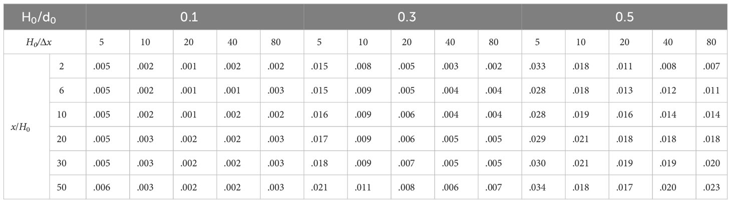
Table 3 L₂ errors of the wave height for water depth 5 m.

Table 4

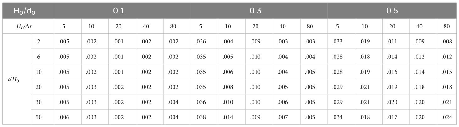
Table 4 L₂ errors of the wave height for water depth 10 m.

$\begin{array}{ll}{L}_2=\sqrt{\frac{1}{N}\sum _{t=0}^N{\left(\frac{h_t^n-h_t^e}{h_t^e}\right)}^2}& (24)\end{array}$

where $h_t^n$ and $h_t^e$ are the numerical result and the analytical solution at time t, respectively; N is the sample numbers.

The L₂ errors decreases and gradually stabilizes with the increase of relative particle spacing. The calculated results with different water depth indicate that the relative error is relatively large with a maximum value of 0.094 for H₀/$\Delta$x = 5. The calculation error is basically stable for H₀/$\Delta$x $\ge$20. The minimum values of L₂ error for relative wave heights 0.1, 0.3, and 0.5 are 0.001, 0.002, and 0.007, respectively. The L₂ error gradually increases with the increase of wave height. The calculation error for the model of H₀/d_{0 =} 0.1 is the smallest with a minimum value 0.001. The maximum error is reached for the model of H₀/d_{0 =} 0.5 with a maximum value of 0.093. For H₀/d_{0 =} 0.1, the water depth has little effect on the calculation error of the model. The calculation error of the SPH model with different water depth is basically the same with a maximum error 0.005 and a minimum error 0.001. For H₀/d_{0 =} 0.3, the calculation error of the model with 1 m water depth is highest with a maximum value 0.094 while the calculation error of the model with 2 m water depth is relatively small and gradually increases with the increase of water depth with a minimum error 0.002 and a maximum error 0.038. For H₀/d_{0 =} 0.5, the calculation error of the model with 1 m water depth is highest with a maximum value of 0.093 while the calculation error of the model with 2 m water depth is relatively small and gradually increases with the increase of water depth with a minimum error 0.007 and a maximum error 0.081. For H₀/d_{0 =} 0.1, the L₂ error gradually increases with the increase of measurement point distance, but the difference is not significant with a maximum difference 0.001 and a minimum difference 0. The L₂ error of the model for H₀/d_{0 =} 0.3 also gradually increases with the increase of measurement point distance with a maximum difference 0.100 and a minimum difference 0. For H₀/d_{0 =} 0.5, the L₂ error of the calculated results also increases with the increase of measurement point distance with a maximum difference 0.016 and a minimum difference 0.

In summary, the model can accurately simulate the propagation of the solitary waves. The calculated results of the SPH model with the relative particle spacing greater than or equal to 20 is in good agreement with the analytical solution. Therefore, the relative particle spacing should be greater than or equal to 20 for the simulation of the solitary waves based on the SPH model. The error of the calculated results gradually increases with the increase of measurement point distance, but the change is not significant with a maximum difference 0.016 of the L₂ error. The influence of water depth on the L₂ error of the calculated results is relatively complex. The water depth has little effect on the calculation results with a small relative wave height. As the relative wave height increases, the calculation error with small water depth (1 m) is larger. The calculation error with water depth greater than or equal to 2 m is smaller and slightly increases with water depth increase. The reason may be that the increase in water depth reduces the relative error.

3.4 Analysis of the attenuation of solitary wave peaks along the distance of measurement points

Figure 6 shows the calculated solitary wave peaks at different measurement points with a relative particle spacing of 20 under different water depths and relative wave heights. The error of calculated solitary wave peaks increases with the increase of relative wave height. The calculated wave peaks with the relative wave height 0.1 are in good agreement with the theoretical value while the wave peaks slightly decrease with the increase of the distance along the measuring point. The error of wave peaks with relative wave height 0.3 is slightly larger. The wave peaks first increase and then decrease with the distance along the measurement point increases. For the relative wave height 0.5, the error of wave peaks is large with that the peak values of the solitary wave also increase and then decrease with the distance along the measurement point increases. The peak value is the highest for x/H_{0 =} 5 and the peak value at the measurement points between 5 and 30 exceeds the analytical value. The calculated wave peaks do not vary significantly with water depth. The calculated results for water depths 1 m and 10 m differ largely from the theoretical values compared to the calculated results for water depths 2 m and 5 m. The errors of calculated wave peaks increase along the measurement points for the model of relative wave height 0.1 while the errors of calculated wave peak decrease and then increase for the model of relative wave heights 0.3 and 0.5 with the smallest error between x/H_{0 =} 2 - 5.

Figure 6

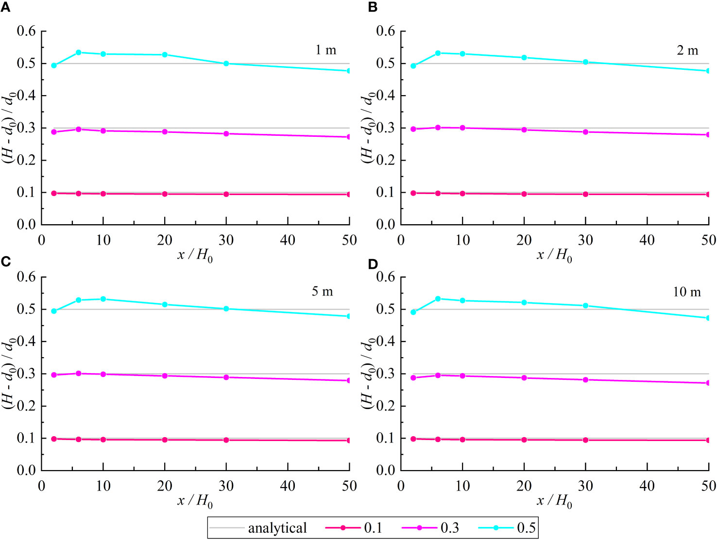
Figure 6 Solitary wave peak along the channel for water depth of 1 m, 2 m, 5 m, and 10 m (A–D).

Table 5 gives the L₂ error of calculated solitary wave peaks for SPH model with different water depths and relative wave heights. The errors of the wave peaks gradually increase with the increase of relative wave height but the increasing value is not significant with a minimum L₂ error 0.033 and maximum L₂ error 0.052. The wave peaks calculated by the SPH model does not vary significantly with water depth. The L₂ errors for the model of water depths 1 m and 10 m are slightly larger with a maximum value 0.052 while it is smaller for the model of water depths 2 m and 5 m with a minimum value 0.033. The standard deviations of calculated solitary wave peaks are given in Table 6. The standard deviations increase with the increase of water depth and wave height, and reach the maximum at the model of water depth 10 m with relative wave height 0.5. The maximum standard deviation is 0.021 while the minimum value is 0.001.

Table 5

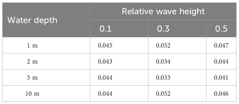
Table 5 L₂ errors of solitary wave peak.

Table 6

Table 6 Standard deviation of solitary wave peak.

In short, the calculated solitary wave peaks with small errors decrease along the measurement points distance. Meanwhile the solitary wave peaks are underestimated slightly for the model with small relative wave heights. As the relative wave heights increases, the calculated wave peaks show a trend of upward and then downward. The calculated results will overestimate the wave peaks within a certain distance in the middle of the channel while the wave peaks will be underestimated at the beginning and end of the channel. The calculated wave peaks do not change significantly with water depth. The errors of the model with the large and small water depths are slightly larger than that the water depth is moderate. The maximum and minimum L₂ errors are 0.052 and 0.033, respectively. The errors of calculated wave peak along the measurement points gradually increase for the model with small relative wave height while the errors first decrease and then increase for the model with large relative wave height. The error is the smallest between x/H_{0 =} 2 - 5.

4 Case study on the interaction between the solitary waves and the semi-submerged structures

4.1 Model validation

A test case of solitary waves interaction with partially submerged rectangular obstacle is simulated to validate the model. The calculated wave heights are compared with the OpenFOAM results (Ma et al., 2019). The numerical flume is 2.0 m height and 100 m length. The initial water depth is 1.0 m. The wave height is 0.1 m. The rectangular structure is 5.0 m × 0.6 m with a center coordinate (32.5 m, 0.9 m). The particle spacing sets to 0.01 m. Figure 7 shows the comparing of wave height between the OpenFOAM results and SPH model at two points x = 1 m and 59 m. The phase and magnitude of the calculated wave height are in well agreement with the OpenFOAM results. The maximum absolute error is 0.004 m with relative error 0.4%.

Figure 7

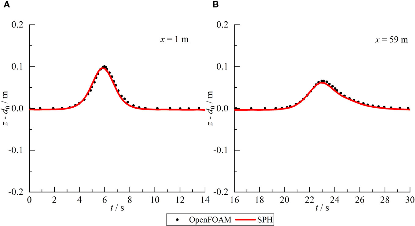
Figure 7 Comparison of the wave surface between SPH results and OpenFOAM results at position of x=1 m (A) and x =59 m (B).

4.2 Model layout

To analyze the characteristics of wave surface, velocity, vorticity, and wave loads of the interaction between solitary waves and semi-submersible structure, a 300 m $\times$ 10 m 2D rectangular numerical wave tank with a semi-submersible platform is adopted. The water depth is d_{0 =} 5.0 m. The size of the semi-submersible platform fixed above the still water surface is 5.0 m $\times$ 0.6 m with center coordinates (52.5 m, 0.9 m). The submerged height (distance from the bottom of the structure to the water surface) of the structure is 0.4 m. The model layout is shown in Figure 8. The relative wave height H₀/d_{0 =} 0.1. The relative particle spacing H₀/$\Delta$x = 50.

Figure 8

Figure 8 Schematic diagrams of the model.

4.3 Wave heights

Figure 9 shows the time history of the wave heights at the upstream (x = 35) and downstream (x = 60) measurement points of the structure. At t = 7 s, the solitary wave arrives the upstream measuring point inducing the wave height to rise. The wave height of upstream measuring point reaches maximum value 0.498 m at t = 15 s. Then the solitary wave continues to propagate downstream through the upstream measuring point, and falls to form a wave surface oscillation. The oscillation gradually attenuates over time. At t = 10 s, the solitary wave crosses the structure and arrives the downstream measuring point inducing the wave height to rise. The solitary wave reaches the maximum value 0.438 m at t = 18 s. Then the wave continues to propagate downstream through the downstream measurement point, and drops with a gradually decaying wave surface oscillation.

Figure 9

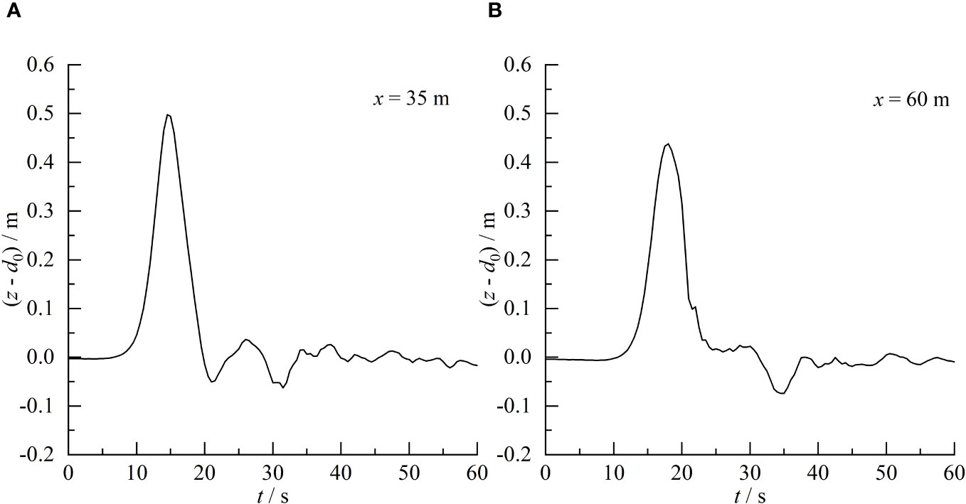
Figure 9 Time history of the wave height at position of x =35 m (A) and x=60 m (B).

Figure 10 gives the time history of the wave heights at the center of the semi-submersible platform x = 52.5 m. The initial wave height is -0.4 m of the platform bottom elevation due to the structure being submerged in water. At t = 16 s, the semi-submersible structure experiences overtopping. The solitary wave climbs to the top of the platform and arrives the measuring point inducing the wave surface to rapidly rise. The changes in wave surface are complex with two double peaks with a peak value of 0.398 m at t = 20 s and a maximum value 0.410 m at t = 33 s due to the fluctuation of the wave surface.

Figure 10

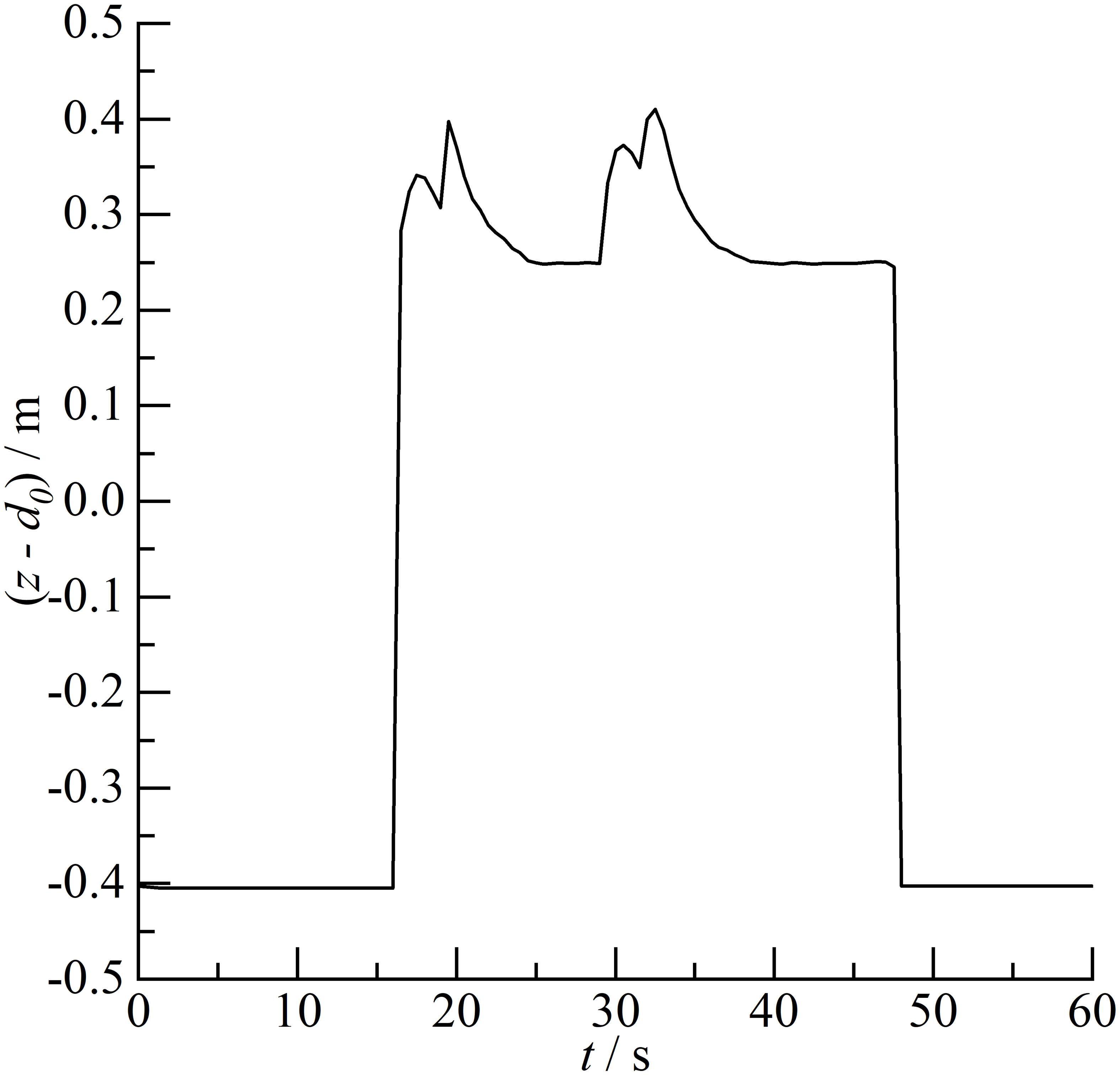
Figure 10 Time history of the wave height at the center of the structure.

4.4 Wave loads

Figures 11 shows the time history of the horizontal and vertical wave loads coefficient C_x and C_z of the semi-submersible structures.

Figure 11

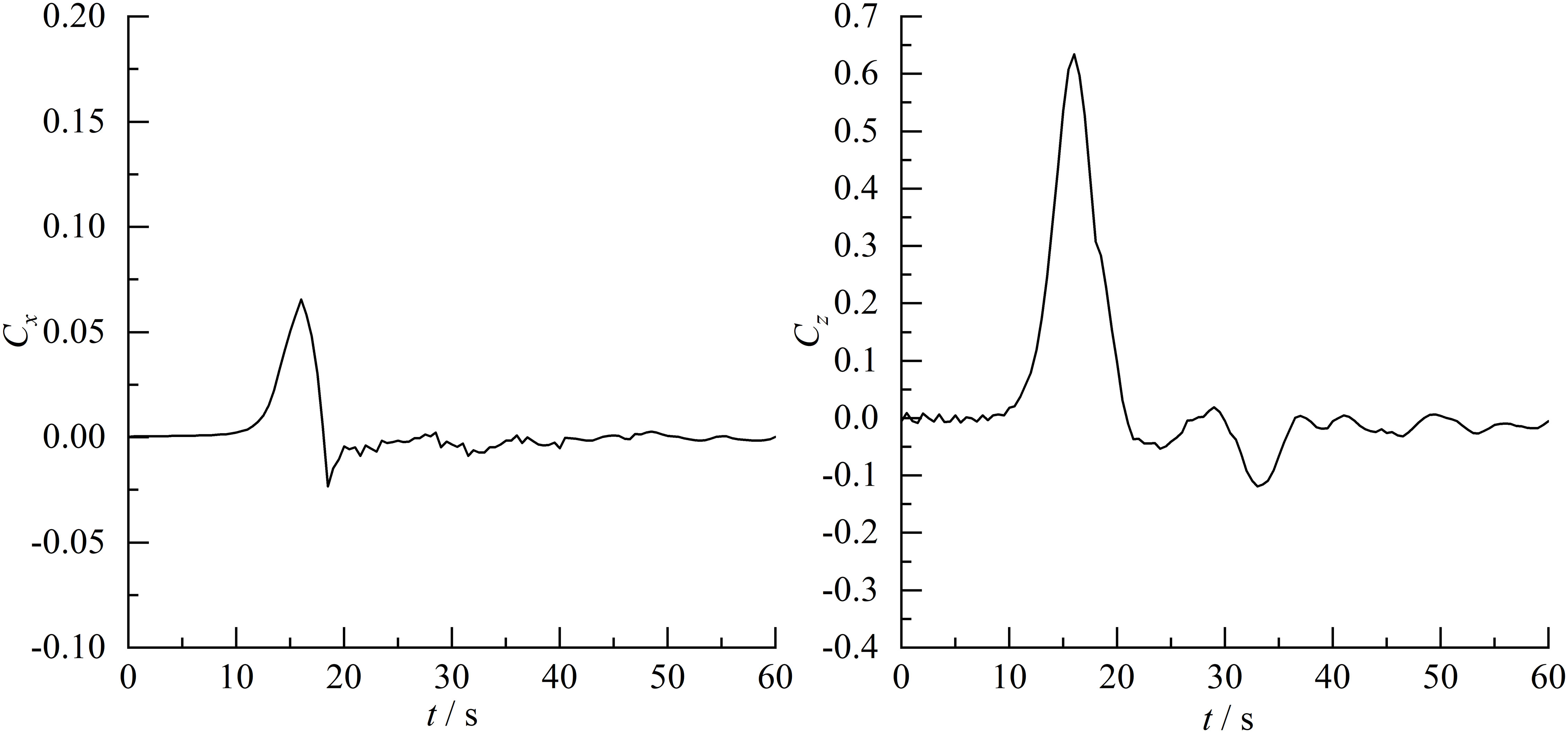
Figure 11 History of wave load coefficient of obstacle.

$\begin{array}{ll}{C}_x=\frac{F_x}{{\rho }_{0}gA}, C_z=\frac{F_z}{{\rho }_{0}gA}& (25)\end{array}$

where, A=0.6 m $\times$ 5 m is the area of the structure;F_x and F_z are the horizontal and vertical wave loads on structures. F_x and F_z are calculated by summing up the force of all the structure particles. The equations are:

$\begin{array}{ll}{\mathit{F}}_a=\frac{d{\mathit{u}}_a}{dt}=-\sum _b{m}_b\left(\frac{P_b}{{\rho }_b^2}+\frac{P_a}{{\rho }_a^2}+{\text{Π}}_{ab}\right){\nabla }_a{W}_{ab}+\mathit{g}& (26)\end{array}$

$\begin{array}{ll}\mathit{F}=m\sum \frac{d{\mathit{u}}_a}{dt}& (27)\end{array}$

where, F(F_x、F_z) is the total force acting on the structure. F_a is the force acting on arbitrary particle a that constitutes the structure.

At t = 10 s, the solitary wave arrives the semi-submersible platform resulting in a rapid increase in the horizontal force. The horizontal wave load reaches the maximum 0.066 at t = 16 s. The horizontal force on the platform rapidly decreased until it reaches the minimum -0.023 at t = 19 s. The horizontal wave load amplitude is 0.089. Then, the solitary wave passes through the structure and continues to propagate downstream. The horizontal wave load also experiences an oscillation with a decreasing amplitude due to the wave surface oscillation induced by the interaction between the solitary waves and the platform. Similar to the horizontal wave loads, the solitary wave arrives the semi-submersible structure at t = 10 s inducing a rapid increase in the vertical wave loads. The vertical wave loads reach the maximum 0.635 at t = 16 s. The vertical forces rapidly decreases until it reaches the minimum -0.053 at t = 24 s. The vertical wave loads amplitude is 0.688. Similarly, the wave surface oscillation also causes an oscillation with a decreasing amplitude in the vertical wave loads due to the interaction between solitary waves and the structure. Obviously, the oscillation amplitude of the vertical wave loads is greater than the horizontal wave loads. In summary, both the horizontal and vertical wave loads on the semi-submersible platform exhibit positive and negative pressures with vertical and horizontal wave loads amplitudes 0.688 and 0.089, respectively. The vertical wave loads are significantly larger than the horizontal wave load. Therefore, the vertical forces on the platform should be the control stress for the structural design.

4.5 Velocity field

The velocity fields around the semi-submersible platform at six different instants are given in Figure 12. In Figure 12, u represents the velocity (m/s) in the x-axis direction. At t = 15 s, the solitary wave arrives the structure and climbs to the top of the structure inducing overtopping. Simultaneously, partial solitary waves pass through the bottom of the structure causing uplift of downstream wave surface. The velocity at the top of the structure is relatively high with a value 1.2 m/s while it is relatively small at the bottom of the structure with a value 0.5 m/s. The downstream wave surface rises and forms overtopping spreading upstream at t = 16 s. The upstream overtopping at the top of the structure increases. The velocity at the top and bottom of the structure increases to1.9 m/s and 0.7 m/s, respectively. Until t = 17.5 s, the solitary wave completely arrives the structure. The upstream wave surface begins to decline while the downstream wave surface continues to rise. The upstream and downstream overtopping approaches and collides to form a hydraulic jump. The velocity at the top and bottom of the structure reaches the maximum value 2.2 m/s and 0.8 m/s. At t = 18.5 s, the solitary wave passes through the structure causing the upstream wave surface to decrease continually and the downstream wave surface to rise continually. The hydraulic jump at the top of the structure develops and propagates upstream. The water at the top of the structure flows into the downstream lead to the decreasing of the overtopping. The velocity at the top and bottom of the structure decreases to 1.6 m/s and 0.7 m/s. Both the upstream and downstream wave surfaces drop at t = 19.5 s. Meanwhile, the overtopping continually flows into downstream flume leading to the declining of the wave surface on the top of the structure. The velocity continues to decrease. The maximum velocity position is transferred to the upper right corner of the structure with a maximum value 1.8 m/s. Until t = 21.5 s, the solitary wave passes through the structure for a certain time. The wave surface around the structure reaches the initial wave surface 5 m again. The interaction between upstream and downstream overtopping is fully developed with only a thin layer of overtopping water continue to flow into the flume from the upstream and downstream of the structure. The velocity further decreases to 1.2 m/s.

Figure 12

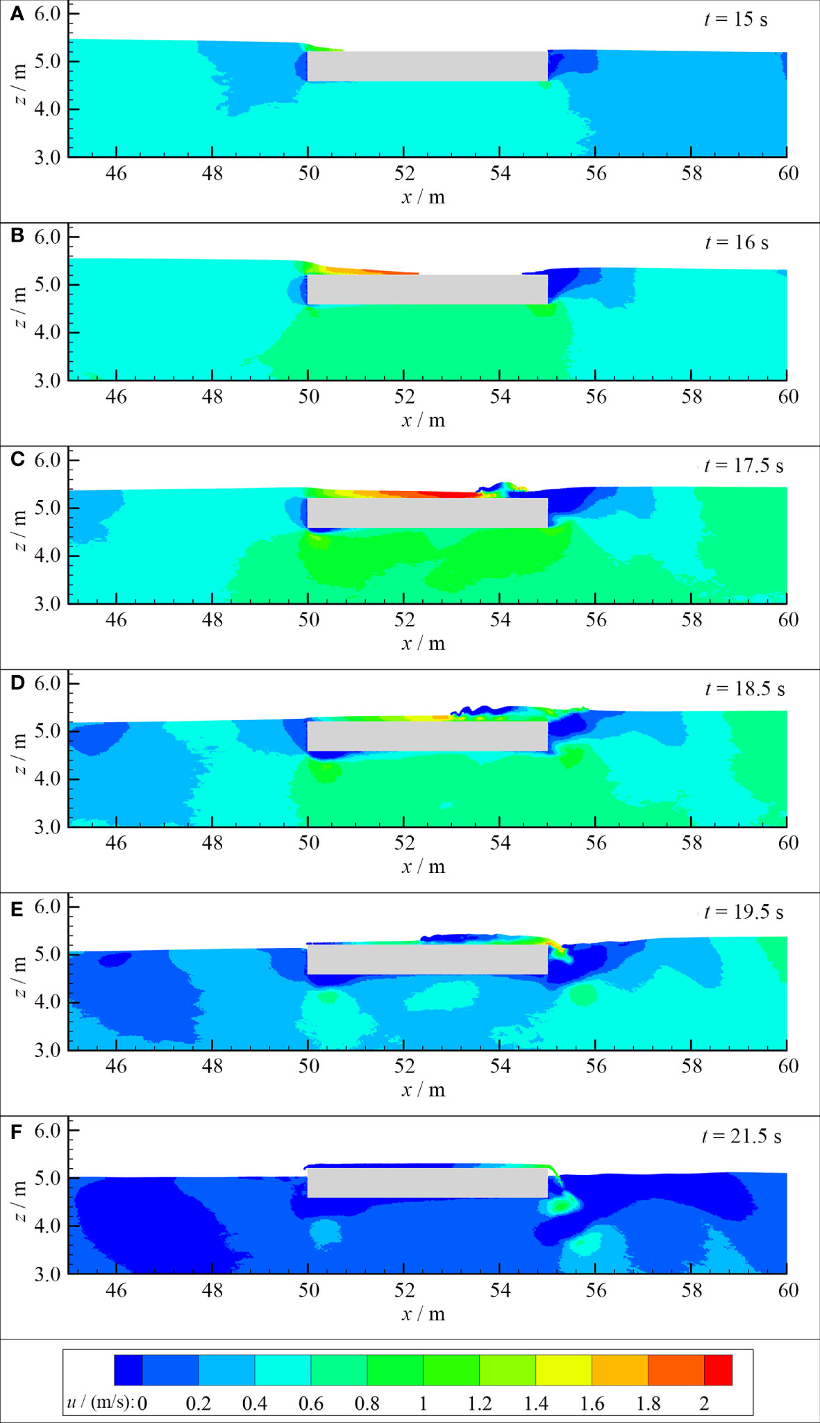
Figure 12 Velocity field of the interaction between solitary wave and semi-submersible platform at t= 15 s, 16 s, 17.5 s, 18.5 s, 19.5 s, and 21.5 s (A–F).

4.6 Vorticity field

The vorticity field of the interaction between solitary wave and semi-submersible platform is given in Figure 13. Vor Y represents vorticity (s^-1) in Y direction. At t = 15 s, the solitary wave arrives the structure and generates a small overtopping. The vorticity appears at the four corners of the structure with positive vorticity in the upper left corner and negative vorticity in the rest. The vorticity at the four corners increases gradually at t = 16 s. Until t = 17.5 s, a large counterclockwise vortex forms at the bottom of the structure leading edge with the maximum intensity -29 s^-1. The vortex intensity at the top of the leading edge of the structure gradually decreases. The vortex on the top of the structure is also complex due to the collision between upstream and downstream overtopping. Positive and negative vortices exist at the same time and change rapidly with the maximum intensity 26 s^-1 and -33 s^-1, respectively. A large counter clockwise vortex appears downstream of the structure with the maximum intensity -8 s^-1. At t = 18.5 s, the anticlockwise vortex at the bottom of the structure leading edge increases and develops to the depth and downstream direction with the maximum intensity -14 s^-1. The vorticity on the top of the structure is further developed and becomes more complex. There are more positive and negative vortex structures and their mixing. The maximum intensity of positive and negative vortices is 16 s^-1 and -40 s^-1. The counter clockwise vortex downstream of the structure develops with increasing area and moves away from the semi-submersible structure. The vortex intensity does not change significantly with the same maximum value -8 s^-1. The anti-clockwise vortex intensity at the bottom of the structure leading edge begins to weaken and continually develops to the depth and downstream direction with the intensity -10 s^-1 at t = 19.5 s. The intensity of the vortex on the top of the structure gradually weakens. The clockwise vortex disappears while only the counterclockwise vortex exists with the intensity -40 s^-1. The counter clockwise vortex area at the downstream of the structure continually increases with the decreased intensity -7 s^-1. Meanwhile, the clockwise vortex appears at the downstream of the structure near the wall with the maximum intensity 28 s^-1. Until t = 21.5 s, the intensity and range of the counterclockwise vortex at the bottom of the structure leading edge decrease rapidly with the maximum intensity -6 s^-1. The vortex on the top of the structure basically disappears. The scope of downstream vortex continues to increase. The intensity of clockwise vortex decreases while the intensity of counterclockwise vortex changes little. The maximum positive and negative vortex intensities are 16 s^-1 and -7 s^-1, respectively. The vortex structure rapidly moves away from the structure toward the downstream and depth.

Figure 13

Figure 13 Vorticity field of the interaction between solitary wave and semi-submersible platform at t= 15 s, 16 s, 17.5 s, 18.5 s, 19.5 s, and 21.5 s (A–F).

5 Conclusions

A meshless solitary waves model which can handle the large deformation and strong nonlinear waves is established based on the SPH method and Rayleigh solitary wave theory. The accuracy of the model is validated by analyzing the consistency between the calculated wave height results and theoretical data as well as the stability of simulated solitary waves. The calculated results of the SPH model with the relative particle spacing ≥ 20 are in good agreement with the analytical solution and has a good stability. The calculation error slightly increases with the increase of measurement point distance, but the change is not significant with a maximum L₂ error difference of 0.016. Therefore, the SPH model can accurately simulate the propagation of the solitary waves.

The results of the interaction between solitary waves and semi-submersible platforms indicate that an overtopping occurs leading to complex wave surface various and wave oscillation. Two double peaks appear at the central measuring point of the platform with maximum wave heights 0.398 m and 0.410 m, respectively. The maximum wave heights at the upstream and downstream measurement point reaches 0.498 m and 0.438 m, respectively. The wave transmission coefficient K_t = 0.880. The horizontal and vertical forces on the semi-submersible platform exhibit positive and negative pressures accompanying wave load amplitudes 0.688 and 0.089, respectively. The vertical load is significantly larger than the horizontal load, and the vertical forces on the platform should be the control stress for the structural design.

A hydraulic jump at the top of the structure is formed due to the interaction between the upstream and downstream overtopping inducing by the solitary waves. The maximum velocities at the top and bottom of the structure are 2.2 m/s and 0.8 m/s, respectively. A large counterclockwise vortex forms at the bottom of the structure leading edge with a maximum intensity -29 s^-1. Both positive and negative vorticity exist simultaneously and rapidly change with the maximum intensity 26 s^-1 and -40 s^-1 at the top of the structure due to the hydraulic jump. Downstream of the structure, a counterclockwise vortex first appears followed by a clockwise vortex with the maximum vortex intensity -8 s^-1 and 28 s^-1, respectively.

Data availability statement

The raw data supporting the conclusions of this article will be made available by the authors, without undue reservation.

Author contributions

JL: Formal Analysis, Methodology, Writing – original draft. LH: Formal Analysis, Writing – original draft. YH: Resources, Visualization, Writing – review & editing. HM: Methodology, Visualization, Writing – review & editing. GW: Methodology, Supervision, Writing – review & editing. ZT: Investigation, Visualization, Writing – review & editing. DZ: Investigation, Visualization, Writing – review & editing.

Funding

The author(s) declare financial support was received for the research, authorship, and/or publication of this article. This work was financially supported by the National Natural Science Foundation of China (Grant No. 52001071); the Guangdong Basic and Applied Basic Research Foundation (Grant No. 2023A1515010890, 2022A1515240039); the Special Fund Competition Allocation Project of Guangdong Science and Technology Department (Grant No. 2021A05227); the Marine Youth Talent Innovation Project of Zhanjiang (Grant No. 2021E05009, 2021E05010); Non-funded Science and Technology Research Program Project of Zhanjiang (Grant No. 2021B01160, 2021B01416); the Doctor Initiate Projects of Guangdong Ocean University (No. 060302072103, R20068); Innovative Team for Structural Optimization of Ocean and Hydraulic Engineering(CXTD2023012).

Conflict of interest

Author DZ was employed by the company Powerchina Hebei Electric Power Engineering CO., LTD.

The remaining authors declare that the research was conducted in the absence of any commercial or financial relationships that could be construed as a potential conflict of interest.

Publisher’s note

All claims expressed in this article are solely those of the authors and do not necessarily represent those of their affiliated organizations, or those of the publisher, the editors and the reviewers. Any product that may be evaluated in this article, or claim that may be made by its manufacturer, is not guaranteed or endorsed by the publisher.

References

Altomare C., Crespo A. J. C., Rogers B. D., Dominguez J. M., Gironella X., Gómez-Gesteira M. (2014). Numerical modelling of armour block sea breakwater with smoothed particle hydrodynamics. Comput. Struct. 130, 34–45. doi: 10.1016/j.compstruc.2013.10.011

CrossRef Full Text | Google Scholar

Aristodemo F., Tripepi G., Meringolo D. D., Veltri P. (2017). Solitary wave-induced forces on horizontal circular cylinders: Laboratory experiments and SPH simulations. Coast. Eng. 129, 17–35. doi: 10.1016/j.coastaleng.2017.08.011

CrossRef Full Text | Google Scholar

Canelas R. B., Domínguez J. M., Crespo A. J. C., Gomez-Gesteira M., Ferreira R. M. L. (2015). A Smooth Particle Hydrodynamics discretization for the modelling of free surface flows and rigid body dynamics. Int. J. Numer. Meth. Fluids. 78, 581–593. doi: 10.1002/fld.4031

CrossRef Full Text | Google Scholar

Chen Q., Zang J., Kelly D. M., Dimakopoulos A. S. (2017). A 3-D numerical study of solitary wave interaction with vertical cylinders using a parallelised particle-in-cell solver. J. Hydrodyn. 29 (5), 790–799. doi: 10.1016/S1001-6058(16)60790-4

CrossRef Full Text | Google Scholar

Constantin A., Escher J., Hsu H. C. (2011). Pressure beneath a solitary water wave: mathematical theory and experiments. Arch. Ration. Mech. Anal. 201 (1), 251–269. doi: 10.1007/s00205-011-0396-0

CrossRef Full Text | Google Scholar

Crespo A. J. C., Domínguez J. M., Rogers B. D., Gomez-Gesteira M., Longshaw S., Canelas R., et al. (2015). DualSPHysics: Open-source parallel CFD solver based on Smoothed Particle Hydrodynamics (SPH). Comput. Phys. Commun. 187, 204–216. doi: 10.1016/j.cpc.2014.10.004

CrossRef Full Text | Google Scholar

Crespo A. J. C., Gómez-Gesteira M., Dalrymple R. A. (2007). Boundary conditions generated by dynamic particles in SPH methods. Comput. Mater. Con. 5, 173–184.

Google Scholar

Cunningham L. S., Pringgana G., Rogers B. D. (2014). Tsunami wave and structure interaction: an investigation with smoothed-particle hydrodynamics. Proc. Inst. Civ. En-Eng. 167, 126–138. doi: 10.1680/eacm.13.00028

CrossRef Full Text | Google Scholar

Dalrymple R. A., Rogers B. D. (2006). Numerical modeling of water waves with the SPH method. Coast. Eng. 53, 141–147. doi: 10.1016/j.coastaleng.2005.10.004

CrossRef Full Text | Google Scholar

Ding W., Ai C., Jin S., Lin J. (2020). Numerical investigation of an internal solitary wave interaction with horizontal cylinders. Ocean Eng. 208, 107430. doi: 10.1016/j.oceaneng.2020.107430

CrossRef Full Text | Google Scholar

Domínguez J. M., Altomare C., Gonzalez-Cao J., LoMonaco P. (2019). Towards a more complete tool for coastal engineering: solitary wave generation, propagation and breaking in an SPH-based model. Coast. Eng. J. 61, 15–40. doi: 10.1080/21664250.2018.1560682

CrossRef Full Text | Google Scholar

Domínguez J. M., Crespo A. J. C., Gómez-Gesteira M., Marongiu J. C. (2011). Neighbour lists in smoothed particle hydrodynamics. Int. J. Numer. Meth. Fluids. 67, 2026–2042. doi: 10.1002/fld.2481

CrossRef Full Text | Google Scholar

Farahani R. J., Dalrymple R. A. (2014). Three-dimensional reversed horseshoe vortex structures under broken solitary waves. Coast. Eng. 91, 261–279. doi: 10.1016/j.coastaleng.2014.06.006

CrossRef Full Text | Google Scholar

Farhadi A., Ershadi H., Emdad H., Rad E. G. (2016). Comparative study on the accuracy of solitary wave generations in an ISPH-based numerical wave flume. Appl. Ocean Res. 54, 115–136. doi: 10.1016/j.apor.2015.11.003

CrossRef Full Text | Google Scholar

Gao J., Ma X., Chen H., Zang J., Dong G. (2021a). On hydrodynamic characteristics of transient harbor resonance excited by double solitary waves. Ocean Eng. 219, 108345. doi: 10.1016/j.oceaneng.2020.108345

CrossRef Full Text | Google Scholar

Gao J., Ma X., Dong G., Chen H., Liu Q., Zang J. (2021b). Investigation on the effects of Bragg reflection on harbor oscillations. Coast. Eng. 170, 103977. doi: 10.1016/j.coastaleng.2021.103977

CrossRef Full Text | Google Scholar

Gao J., Ma X., Dong G., Zang Z., Ma Y., Zhou L. (2019). Effects of offshore fringing reefs on the transient harbor resonance excited by solitary waves. Ocean Eng. 190, 106422. doi: 10.1016/j.oceaneng.2019.106422

CrossRef Full Text | Google Scholar

Gao J., Ma X., Zang J., Dong G., Ma X., Zhu Y., et al. (2020). Numerical investigation of harbor oscillations induced by focused transient wave groups. Coast. Eng. 158, 103670. doi: 10.1016/j.coastaleng.2020.103670

CrossRef Full Text | Google Scholar

Gao J., Shi H., Zang J., Liu Y. (2023). Mechanism analysis on the mitigation of harbor resonance by periodic undulating topography. Ocean Eng. 281, 114923. doi: 10.1016/j.oceaneng.2023.114923

CrossRef Full Text | Google Scholar

Geng T., Liu H., Dias F. (2021). Solitary-wave loads on a three-dimensional submerged horizontal plate: Numerical computations and comparison with experiments. Phys. Fluids. 33, 037129. doi: 10.1063/5.0043912

CrossRef Full Text | Google Scholar

Gomez-Gesteira M., Rogers B. D., Crespo A. J. C., Dalrymple R. A., Narayanaswamy M., Dominguez J. M. (2012). SPHysics – development of a free-surface fluid solver – Part 1: Theory and formulations. Comput. Geosci. 48, 289–299. doi: 10.1016/j.cageo.2012.02.029

CrossRef Full Text | Google Scholar

Guizien K., Barthélemy E. (2002). Accuracy of solitary wave generation by a piston wave maker. J. Hydraul. Res. 40, 321–331. doi: 10.1080/00221680209499946

CrossRef Full Text | Google Scholar

Ha T., Shim J., Lin P., Cho Y. (2014). Three-dimensional numerical simulation of solitary wave run-up using the IB method. Coast. Eng. 84, 38–55. doi: 10.1016/j.coastaleng.2013.11.003

CrossRef Full Text | Google Scholar

He M., Khayyer A., Gao X., Xu W., Liu B. (2021). Theoretical method for generating solitary waves using plunger-type wavemakers and its Smoothed Particle Hydrodynamics validation. Appl. Ocean Res. 106, 102414. doi: 10.1016/j.apor.2020.102414

CrossRef Full Text | Google Scholar

He M., Liang D. F., Ren B., Li J., Shao S. (2023). Wave interactions with multi-float structures: SPH model, experimental validation, and parametric study. Coast. Eng. 184, 104333. doi: 10.1016/j.coastaleng.2023.104333

CrossRef Full Text | Google Scholar

He J. H., Qie N., He C. H. (2021). Solitary waves travelling along an unsmooth boundary. Results Phys. 24, 104104. doi: 10.1016/j.rinp.2021.104104

CrossRef Full Text | Google Scholar

Higuera P., Liu P. L. F., Lin C., Wong W. Y., Kao M. J. (2018). Laboratory-scale swash flows generated by a non-breaking solitary wave on a steep slope. J. Fluid Mech. 847, 186–227. doi: 10.1017/jfm.2018.321

CrossRef Full Text | Google Scholar

Hsiao S. C., Lin T. C. (2010). Tsunami-like solitary waves impinging and overtopping an impermeable seawall: Experiment and RANS modeling. Coast. Eng. 57 (1), 1–18. doi: 10.1016/j.coastaleng.2009.08.004

CrossRef Full Text | Google Scholar

Hunt-Raby A. C., Borthwick A. G. L., Stansby P. K., Taylor P. H. (2011). Experimental measurement of focused wave group and solitary wave overtopping. J. Hydraul. Res. 49 (4), 450–464. doi: 10.1080/00221686.2010.542616

CrossRef Full Text | Google Scholar

Li J., Liu H., Gong K., Tan S. K. (2012). SPH modeling of solitary wave fissions over uneven bottoms. Coast. Eng. 60, 261–275. doi: 10.1016/j.coastaleng.2011.10.006

CrossRef Full Text | Google Scholar

Lo H. Y., Liu L. F. (2014). Solitary waves incident on a submerged horizontal plate. J. Waterw. Port C-ASCE. 140 (3), 04014009. doi: 10.1061/(ASCE)WW.1943-5460.0000236

CrossRef Full Text | Google Scholar

Ma X., Zheng Z., Gao J., Wu H., Dong Y., Dong G. (2021). Experimental investigation of transient harbor resonance induced by solitary waves. Ocean Eng. 230, 109044. doi: 10.1016/j.oceaneng.2021.109044

CrossRef Full Text | Google Scholar

Ma Y., Yuan C., Ai C., Dong G. (2019). Comparison between a non-hydrostatic model and OpenFOAM for 2D wave-structure interactions. Ocean Eng. 183, 419–425. doi: 10.1016/j.oceaneng.2019.05.002

CrossRef Full Text | Google Scholar

Mahmoudof S. M., Azizpour J. (2020). Field observation of wave reflection from plunging cliff coasts of chabahar. Appl. Ocean Res. 95, 102029. doi: 10.1016/j.apor.2019.102029

CrossRef Full Text | Google Scholar

Mahmoudof S. M., Eyhavand-Koohzadi A., Bagheri M. (2021). Field study of wave reflection from permeable rubble mound breakwater of Chabahar Port. Appl. Ocean Res. 114, 102786. doi: 10.1016/j.apor.2021.102786

CrossRef Full Text | Google Scholar

Mahmoudof S. M., Hajivalie F. (2021). Experimental study of hydraulic response of smooth submerged breakwaters to irregular waves. Oceanologia. 05, 002. doi: 10.1016/j.oceano.2021.05.002

CrossRef Full Text | Google Scholar

Malek-Mohammadi S., Testik F. Y. (2015). New methodology for laboratory generation of solitary waves. J. Waterw. Port C-ASCE. 136 (5), 286–294. doi: 10.1061/(ASCE)WW.1943-5460.0000046

CrossRef Full Text | Google Scholar

Monaghan J. J. (1992). Smoothed particle hydrodynamics. Annu. Rev. Astron. Astr. 30, 543–574. doi: 10.1146/annurev.aa.30.090192.002551

CrossRef Full Text | Google Scholar

Omidvar P., Stansby P. K., Rogers B. D. (2012). Wave body interaction in 2D using smoothed particle hydrodynamics (SPH) with variable particle mass. Int. J. Numer. Meth. Fluids. 68, 686–705. doi: 10.1002/fld.2528

CrossRef Full Text | Google Scholar

Pan K., IJzermans R. H. A., Jones B. D., Thyagarajan A., wan Beest B. W. H., Williams J. R. (2015). Application of the SPH method to solitary wave impact on an offshore platform. Comp. Part. Mech. 3, 155–166. doi: 10.1007/s40571-015-0069-0

CrossRef Full Text | Google Scholar

Qu K., Ren X. Y., Kraatz S. (2017). Numerical investigation of tsunami-like wave hydrodynamic characteristics and its comparison with solitary wave. Appl. Ocean Res. 63, 36–48. doi: 10.1016/j.apor.2017.01.003

CrossRef Full Text | Google Scholar

Rastgoftar E., Jannat M. R. A., Banijamali B. (2018). An integrated numerical method for simulation of drifted objects trajectory under real-world tsunami waves. Appl. Ocean Res. 73, 1–16. doi: 10.1016/j.apor.2018.01.013

CrossRef Full Text | Google Scholar

Saghatchi R., Ghazanfarian J., Gorji-Bandpy M. (2014). Numerical simulation of water-entry and sedimentation of an elliptic cylinder using smoothed-particle hydrodynamics method. J. Offshore Mech. Arct. 136, 031801. doi: 10.1115/1.4026844

CrossRef Full Text | Google Scholar

Sampath R., Montanari N., Akinci N., Prescott S., Smith C. (2016). Large-scale solitary wave simulation with implicit incompressible sph. J. Ocean Eng. Mar. Energy. 2, 313–329. doi: 10.1007/s40722-016-0060-8

CrossRef Full Text | Google Scholar

Tang J., Causon D., Mingham C., Qian L. (2013). Numerical study of vegetation damping effects on solitary wave run-up using the nonlinear shallow water equations. Coast. Eng. 75 (5), 21–28. doi: 10.1016/j.coastaleng.2013.01.002

CrossRef Full Text | Google Scholar

Wang G., Dong G., Perlin M., Ma X., Ma Y. (2011). Numerical investigation of oscillations within a harbor of constant slope induced by seafloor movements. Ocean Eng. 38, 2151–2161. doi: 10.1016/j.oceaneng.2011.09.033

CrossRef Full Text | Google Scholar

Wang Y., Xu F., Zhang Z. (2020). Numerical simulation of inline forces on a bottom-mounted circular cylinder under the action of a specific freak wave. Front. Mar. Sci. 7, 585240. doi: 10.3389/fmars.2020.585240

CrossRef Full Text | Google Scholar

Wang G., Zheng J. H., Maa J. P. Y., Zhang J. S., Tao A. F. (2013). Numerical experiments on transverse oscillations induced by normal-incident waves in a rectangular harbor of constant slope. Ocean Eng. 57, 1–10. doi: 10.1016/j.oceaneng.2012.09.010

CrossRef Full Text | Google Scholar

Wu Y. T., Hsiao S. C. (2018). Generation of stable and accurate solitary waves in a viscous numerical wave tank. Ocean Eng. 167, 102–113. doi: 10.1016/j.oceaneng.2018.08.043

CrossRef Full Text | Google Scholar

Wu N. J., Hsiao S. C., Chen H. H., Yang R. Y. (2016). The study on solitary waves generated by a piston-type wave maker. Ocean Eng. 117, 114–129. doi: 10.1016/j.oceaneng.2016.03.020

CrossRef Full Text | Google Scholar

Wu Y. T., Hsiao S. C., Huang Z. C., Hwang K. S. (2012). Propagation of solitary waves over a bottom-mounted barrier. Coast. Eng. 62, 31–47. doi: 10.1016/j.coastaleng.2012.01.002

CrossRef Full Text | Google Scholar

Wu N. J., Tsay T. K., Chen Y. Y. (2014). Generation of stable solitary waves by a piston-type wave maker. Wave Motion 51 (2), 240–255. doi: 10.1016/j.wavemoti.2013.07.005

CrossRef Full Text | Google Scholar

Wu Y. T., Yeh C. L., Hsiao S. C. (2014). Three-dimensional numerical simulation on the interaction of solitary waves and porous breakwaters. Coast Eng. 85, 12–29. doi: 10.1016/j.coastaleng.2013.12.003

CrossRef Full Text | Google Scholar

Xuan R. T., Wu W., Liu H. (2013). An experimental study on runup of two solitary waves on plane beaches. J. Hydrodyn. 25 (2), 317–320. doi: 10.1016/S1001-6058(13)60369-8

CrossRef Full Text | Google Scholar

Zhang J., Zheng J., Jeng D. S., Guo Y. (2015). Numerical simulation of solitary-wave propagation over a steady current. J. Waterw. Port C-ASCE. 141 (3), 04014041. doi: 10.1061/(ASCE)WW.1943-5460.0000281

CrossRef Full Text | Google Scholar