Efficient 3D real-time adaptive AUV sampling of a river plume front

The coastal environment faces multiple challenges due to climate change and human activities. Sustainable marine resource management necessitates knowledge, and development of efficient ocean sampling approaches is increasingly important for understanding the ocean processes. Currents, winds, and freshwater runoff make ocean variables such as salinity very heterogeneous, and standard statistical models can be unreasonable for describing such complex environments. We employ a class of Gaussian Markov random fields that learns complex spatial dependencies and variability from numerical ocean model data. The suggested model further benefits from fast computations using sparse matrices, and this facilitates real-time model updating and adaptive sampling routines on an autonomous underwater vehicle. To justify our approach, we compare its performance in a simulation experiment with a similar approach using a more standard statistical model. We show that our suggested modeling framework outperforms the current state of the art for modeling such spatial fields. Then, the approach is tested in a field experiment using two autonomous underwater vehicles for characterizing the three-dimensional fresh-/saltwater front in the sea outside Trondheim, Norway. One vehicle is running an adaptive path planning algorithm while the other runs a preprogrammed path. The objective of adaptive sampling is to reduce the variance of the excursion set to classify freshwater and more saline fjord water masses. Results show that the adaptive strategy conducts effective sampling of the frontal region of the river plume.

1 Introduction

Human activities and pollution are heavily impacting the world’s oceans (Halpern et al., 2008). Anthropogenic climate change and local intrusion from industries can lead to fundamentally altered ocean ecosystems, challenging species distributions, loss in biodiversity, incidence of disease, and more (Hoegh-Guldberg and Bruno, 2010; Doney et al., 2012). The changes in ecosystem structure further influence important services such as carbon sequestration, oxygen production, and nutrient food chains. In order to achieve a more sustainable utilization of marine resources and services, we need to enhance our insight. Developing smart technologies for efficient monitoring of the ocean can provide information that enables us to identify adverse effects and guide development of countermeasures, and it can hence be vital in saving or maintaining local ecosystems. Commonly used ocean observation technologies are buoys, drifters, satellites, unmanned surface vehicles, Argo floats, underwater gliders, cabled seafloor observatories, autonomous underwater vehicles (AUVs), hadal landers, or some coupled system of these technologies (see, e.g., Lin and Yang (2020) for an overview). Ocean monitoring systems are advancing from simple and static single sensors systems to dynamic and multisensor systems that can cover a large spectrum of temporal and spatial scales. With the drive in artificial intelligence and robotic systems, there is also a development toward intelligent sampling systems where observations of various kinds are gathered and processed where and when it is considered valuable.

With the improved affordability and functionality of AUVs, the research literature has seen many advances lately; Zhang et al. (2012; 2013) used deterministic algorithms to map coastal temperature upwellings; Das et al. (2015) demonstrated AUV mission planning for informative plankton sampling; Fossum et al. (2018) monitored large temperature gradients by adaptively choosing surveys paths that substantially reduce the uncertainty in the statistical temperature model; Fossum et al. (2019) conducted a 3D AUV survey for chlorophyll-a mapping; Mo-Bjørkelund et al. (2020) employed hexagonal grids for equilateral survey paths to adaptively explore large temperature gradients; Foss et al. (2022) used a 2D spatiotemporal model onboard an AUV to supervise mining waste seafill; Fonseca et al. (2023) compared satellite imagery and adaptive AUV sampling results for predicting algal blooms. These examples from recent research activity have advanced the field of ocean monitoring with AUVs by going from planar (sea-surface) fields to volumetric fields, in the combination of various data sources, or by presenting a novel algorithm for adaptive exploration.

Considering the vastness of our ocean, it is extremely difficult to obtain sufficient data to cover the full range of scale and resolution desired. Instead, one must rely on a combination of different data sources and sophisticated modeling tools. To fill in the gaps effectively, one can further proactively plan targeted and high-precision sampling campaigns that will improve predictions and support decision-making. At its core, these tasks relate to statistical methods that can combine various data sources for prediction and for evaluating data sampling designs to optimize further data-gathering efforts.

In this work, we combine the fields of oceanography, statistics, and robotics to effectively monitor freshwater frontal regions of river outlets in three dimensions (north, east, depth) using AUVs. Specifically, we conduct sampling in the Nidelva River running into the fjord outside Trondheim, Norway (see Figure 1). The freshwater coming from the river is mixing slowly with the more saline fjord waters, which can cause a sharp gradient between the different water masses.

Figure 1

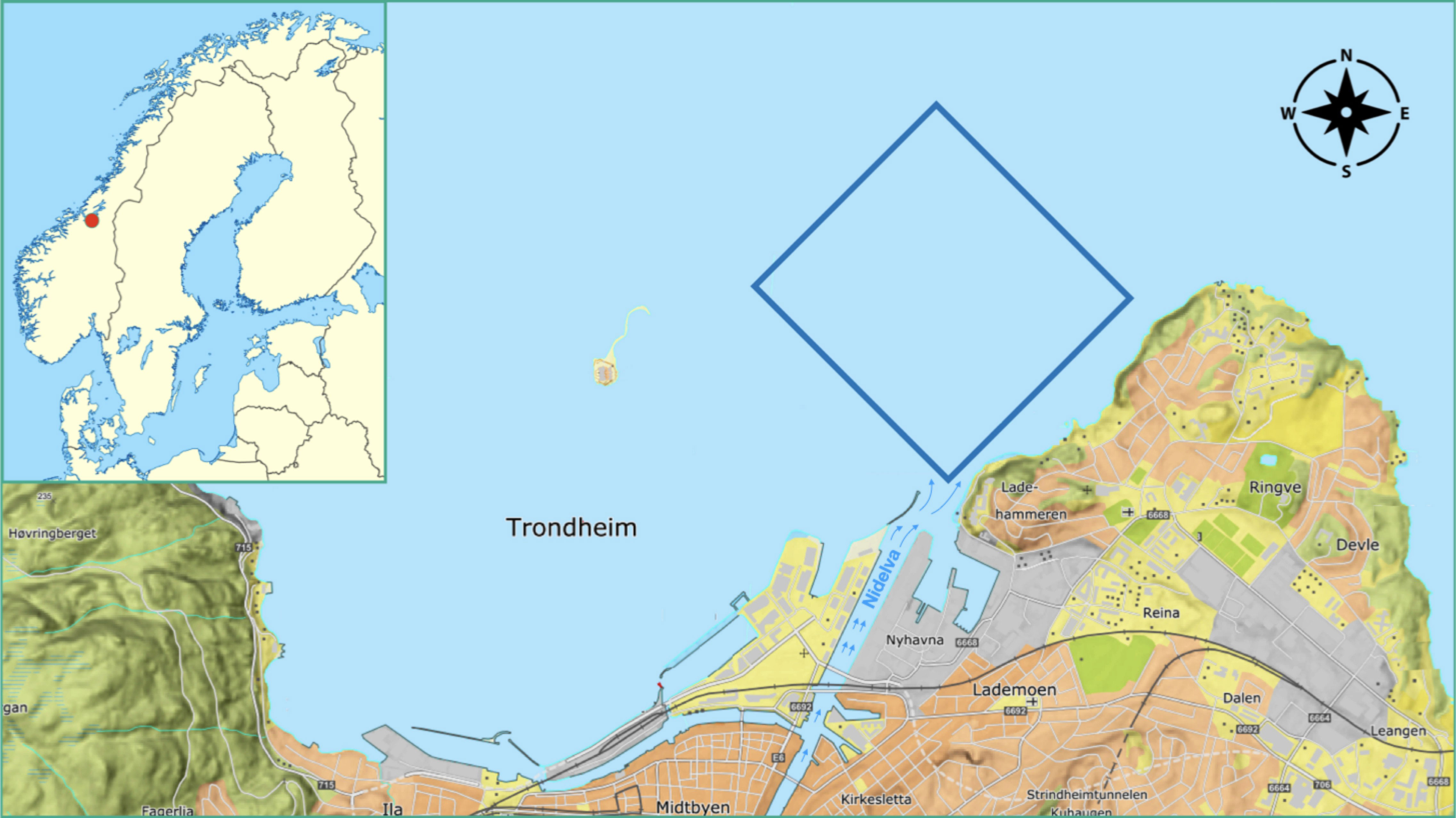
Figure 1 Map of the operational area in the fjord outside Trondheim, Norway. The location of Trondheim is indicated by the red circle on the map of Scandinavia in the top left corner. We have 3D numerical ocean model data at a high lateral and depth resolution in these coastal waters. The blue square just north of the Nidelva River outlet indicates the boundaries of the autonomous underwater vehicle mission in a map view. The operation domain extends from the sea surface to 5-m depth.

At our availability, we have output from a complex numerical ocean model Slagstad and McClimans (2005), henceforth referred to as SINMOD. Along with many other physical oceanography variables, SINMOD outputs salinity at every grid node in a dense spatial (3D) and temporal grid. Even though this model carries much physical insight, the salinity output can be systematically biased, and we will calibrate and update the salinity by deploying an AUV. In this way, the SINMOD data are used to form a prior model for the salinity trends and variations at the time of the AUV deployment. We fit a Gaussian process prior as a surrogate model to the numerical ocean model SINMOD. This surrogate model has the advantage that it can be updated onboard the AUV, and it can hence assimilate in-situ data efficiently. Moreover, this surrogate model enables fast evaluation of various AUV sampling designs in real time whereas it is maneuvering in the water. Fossum et al. (2021) used similar methods to fit a surrogate model from SINMOD, but only in 2D space. Ge et al. (2023) used a 3D Gaussian surrogate prior model, but only for a small-size grid and assuming a much simpler spatial dependency structure.

This paper brings together many elements, and the novelty lies in a more realistic description of spatial correlations with a complex model learned from SINMOD data (Berild and Fuglstad, 2023). The approach is made computationally feasible through modern techniques using a 3D Gaussian random fields with a Markov property, and this enables adaptive AUV sampling based on the new surrogate model in a large-size 3D waypoint graph used during AUV deployments. Additionally, we

● fit the more realistic 3D statistical model to 3D numerical ocean data, and develop a fast algorithm for updating this model onboard an AUV during field deployment,

● develop methods for adaptive path-planning in the context of 3D space with the more realistic model onboard the AUV,

● show through a simulation study, based on SINMOD, that the more realistic statistical model allows an AUV to sample and map the ocean domain better than with a standard statistical model,

● run two AUVs simultaneously in the ocean and show that the combination of an intelligent adaptive survey design and the more realistic model outperforms a standard pre-scripted AUV sampling plan.

In Section 2, we describe the numerical ocean model and its statistical surrogate model. In Section 3, we present the data assimilation part and our approach for adaptive AUV sampling designs. In Section 4, we study properties of the suggested methods in a simulation study. In Section 5, we show results of deployments with one adaptive AUV mission and one preprogrammed mission. In Section 6, we conclude and point to future work.

2 Prior model for salinity

Consider a three-dimensional ocean domain $\mathcal{D}\subseteq {ℝ}^3$, where x(s) represents the salinity field at a specific location $s={(\mathrm{latitude},\mathrm{longitude},\mathrm{depth})}^T \in \mathcal{D}$. The salinity in this ocean domain exhibits both spatial and temporal variations. However, we focus on short-term AUV deployments and simplify our analysis by excluding temporal effects.

2.1 Numerical ocean model

An approximation of the salinity field is achieved using the complex numerical ocean model SINMOD, developed by SINTEF ocean (Slagstad and McClimans, 2005). SINMOD is a three-dimensional model based on the primitive equations, solved using finite difference methods on a regular grid with horizontal cell sizes of 20 km × 20 km, which are nested in several steps down to 32m × 32m for the bay outside Trondheim. The model employs varying vertical resolutions, allowing for higher resolution near the dynamic surface and more uniform resolution in deeper waters. Atmospheric forces (obtained from forecasts available at https://www.met.no), freshwater outflows (data from HBV model (Beldring et al., 2003) provided by the Norwegian Water Resources and Energy Directorate (NVE)), and tides (https://www.tpxo.net/) drive the model. SINMOD offers numerical simulations of multiple ocean variables, including temperature and currents as well as salinity. It is a multipurpose tool that has been used for instance in the prediction of Arctic ocean primary production by leveraging physical–biological coupling (Slagstad et al., 2015; Vernet et al., 2021), in quantifying the effects of the aquaculture structures for large-scale cages by specifying and incorporating drag parameters in SINMOD (Broch et al., 2020), and coupled with the particle dispersion of waste from fish farming (Broch et al., 2017), oil production (Nepstad et al., 2022), or mine tailings (Berget et al., 2018; Nepstad et al., 2020; Berget et al., 2023). For a more comprehensive explanation of the SINMOD methodology, readers are directed to Slagstad and McClimans (2005).

In the current paper, we are only using the salinity outputs from SINMOD. Figure 2 shows an example of SINMOD salinity data and an excursion set (salinity ≤25.4 g/kg) separating water masses into freshwater/saltwater in the fjord outside Trondheim. We notice that the river plume has lower salinity than the surrounding brackish water. There are very low salinity levels (around 5 g/kg–10 g/kg) in the river outlet, whereas the salinity increases further out in the fjord (around 31 g/kg). The temporal resolution of the SINMOD numerical model used for these simulations is 10 min. Salinity is measured in grams salinity per kilogram water (g/kg), which is dimensionless and equal to ‰ and sometimes referred to as the practical salinity unit (PSU).

Figure 2

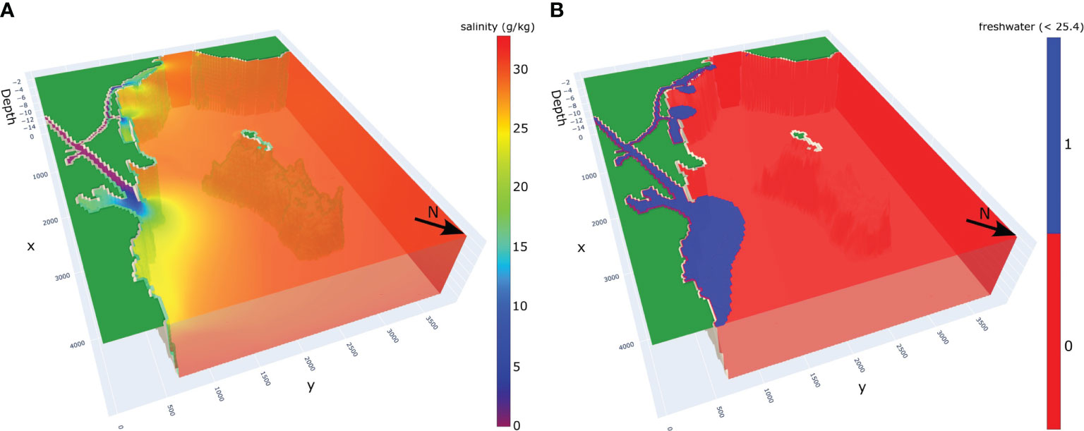
Figure 2 Salinity simulation (A) and corresponding freshwater excursion (B) from the numerical ocean model SINMOD for 08/09/2022.

2.2 Surrogate model with spatially varying anisotropy

In-situ salinity observations made with an AUV are assumed to be more accurate than the forecast provided by SINMOD. However, an AUV measurement only characterizes the salinity at the specific location where the measurement was taken, whereas a model like SINMOD or similar is required to extrapolate variables in space and time. For onboard computing, SINMOD is however too computationally intensive, and it is challenging to assimilate AUV observations in real time with a full-fledged numerical ocean model. Instead, a surrogate model can be trained from the numerical model. It forms an approximate representation of the underlying physical model and is highly applicable for different tasks that require fast updating. Statistical models with spatial effects have shown very suitable for such a task (Gramacy, 2020), and we employ a particular statistical surrogate model for the numerical ocean model salinity data here.

We use the spatial statistical model presented in Berild and Fuglstad (2023), where the 3D salinity field is modeled as a Gaussian Markov random field (GMRF) that allows sparse matrix computations and realistic modeling via spatial variability in the directional dependencies and the variance components. This model is an extension of Lindgren et al. (2011) and Fuglstad et al. (2015).

Assuming that the 3D discretization of the domain $\mathcal{D}\subseteq {ℝ}^3$ consists of n₁×n₂×n₃ grid cells, the salinity field, x(s), is represented by a vector of concatenated field values of size n = n₁n₂n₃. In the application, we have n_{1 =} 50, n_{2 =} 45, n_{3 =} 6 with 32 × 32 m² lateral resolution and 1-m depth resolution. The vector x of salinity values is modeled by a Gaussian distribution, i.e.,

$\begin{array}{ll}\mathit{\text{x}}\sim {\mathcal{N}}_n\left(\mathit{\mu },\mathbf{\Sigma }\right), \mathbf{\Sigma }={\mathbf{Q}}^{-1}.& (1)\end{array}$

Here, the ∼ symbol means “distributed according to,” and ${\mathcal{N}}_n\left(\mathbf{\mu },\mathbf{\Sigma }\right)$ refers to the n-variate Gaussian (or normal) distribution with mean vector µ and covariance matrix Σ, where its inverse, namely, the precision matrix, is denoted Q.

There is much flexibility in choosing the mean vector and covariance matrix in Equation (1), and the Gaussian distribution can hence form quite realistic surrogate models. The mean vector µ of the salinity field captures the spatial trends of the field, which in our case entails fresher water near the river gradually getting more saline going out in the fjord. To form a realistic covariance structure, the idea of Berild and Fuglstad (2023) is to form a random process for u = x−µ via differential operators and Gaussian noise forming a stochastic partial differential equation (SPDE) as

$\begin{array}{ll}({\kappa }^2(s)-\nabla ·\mathbf{\text{H}}(s)\nabla )u(s)=\mathcal{W}(s).& (2)\end{array}$

Here, s is a location in the domain of interest $\mathcal{D}\subseteq {ℝ}^3$ , u(s) is the spatially varying deviation from the trend, and and $\mathcal{W}\left({s}\right)$ is a Gaussian white noise process (with zero mean and statistically independent values), where as $\kappa \left(\mathbf{s}\right)=\kappa \left(\mathit{s};\mathit{\theta }\right)>0$ and $\mathbf{\text{H}}\left(\mathit{s}\right)=\mathbf{H}\left(\mathit{s};\mathit{\theta }\right)>0$ as differentiable are model components controlled by parameters θ that regulate the variability and dependency within the process.

Equation (2) is solved locally for the zero-mean random field u(s) using numerical integration and differentiation on a discretization of the domain of interest $\mathcal{D}$. The solution is $\mathit{u}\sim {\mathcal{N}}_n\left(\mathbf{0},{\mathbf{\text{Q}}}^{-1}\right)$, where the precision matrix $\mathbf{Q}=\mathbf{Q}\left(\mathbf{\theta }\right)$ inherits the sparsity of the differential operators in Equation (2), and it describes the Markov structure in the GMRF model. This structure is very important for our purposes because it enables fast matrix factorization and matrix-vector computations. Hence, the GMRF formulation means that we can update the model onboard the AUV. It is also used in the sampling design evaluations. Without this sparsity, the Gaussian surrogate model could not scale up the magnitude of the ocean mass in 3D (Berild and Fuglstad, 2023).

A detailed description of the model is provided in the Supplementary Material.

2.3 Parameter estimation for salinity field

In order to estimate the parameters and components of the statistical GMRF model for salinity, we utilize numerical ocean model data from SINMOD as the training dataset. These data are denoted as $y({\mathit{s}}_i,t_j)$, where ${\mathit{s}}_i\in \mathcal{D}$ represents the location of cell i ∈ [1,…,n] at time $t_j$ for SINMOD realization j = 1,…,T. The surrogate data model is then

$$y\left({\mathit{s}}_i\right)\sim \mathcal{N}\left(x\left({\mathit{s}}_i\right),{\sigma }_{\mathit{S}}^2\right), i=1,...,n,$$

where ${\sigma }_{\text{S}}^2$ is an unstructured noise variance of the SINMOD dataset.

We estimate a location-dependent mean µ(s_i) of the GMRF using the empirical average across all replicates t_j as:

$\begin{array}{ll}\widehat{\mu }({\mathit{s}}_i)=\frac{1}{T}\sum _{j=1}^{T}y({\mathit{s}}_i,t_j),\text{∀}{\mathit{s}}_i\in \mathcal{D}.& (3)\end{array}$

We compute an estimate $\widehat{\mathit{\theta }}$ of the covariance parameters of the GMRF by maximizing the likelihood function ${L}\left(\mathit{\theta }\right)$, given residual data from an autoregressive model fitted to the SINMOD data [see Supplementary Material and (Berild and Fuglstad, 2023)]. In Sections 4 and 5, the covariance parameters of the models are estimated using a dataset from the SINMOD model, which spans 144 timesteps over the course of 1 day with a temporal resolution of 10 min. This dataset includes observations for all locations within the spatial field at each timestep. Optimizing the likelihood of this rather sophisticated covariance model is not straightforward, but it gets less difficult with more data and this also improves the accuracy of estimates. Berild and Fuglstad (2023) suggest that at least 10 timesteps of the whole field should be used to find reasonable parameter values for such a flexible model.

Figure 3 shows the prior mean (Equation (3)), the prior variance of the n-variate Gaussian distribution $\mathit{x}$, and the corresponding spatial correlation of the marked location. The mean salinity clearly increases going north in the fjord, away from the river outlet. The salinity variance is larger near the river. For the correlation, we notice non-circular contours indicative of anisotropy. Here, the correlation appears to be stronger in the directions where salinity is expected to be similar to that of the reference location.

Figure 3

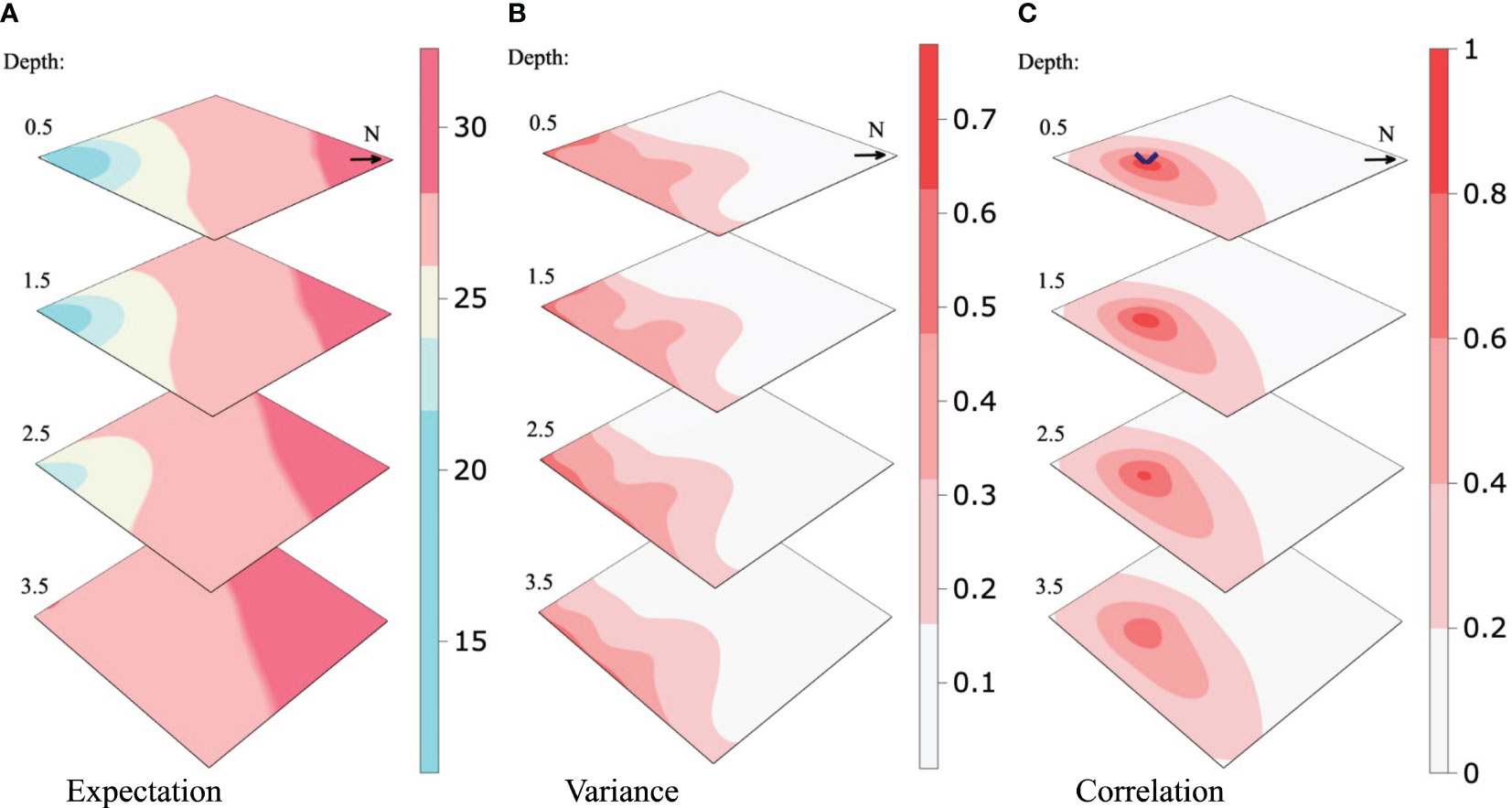
Figure 3 Prior expectation (A), the variance of the process model (B), and the spatial correlation of the location highlighted (C). The N-arrow is the cardinal north.

3 Adaptive AUV sampling

We now delve into our approach for adaptive AUV exploration. One part of this involves continuous updates of the GMRF surrogate model through onboard data assimilation of the in-situ AUV salinity data. Another part is the strategic planning of the next AUV sampling locations.

3.1 Conditioning to AUV data

Assume that the AUV gathers in-situ data at $m$ locations or design points $\mathit{d}=\left\{{\mathit{d}}_1,...,{\mathit{d}}_m\right\}$, where ${\mathit{d}}_j\in \mathcal{D}$. In practice, these locations form an AUV design (a trajectory). Data $y({\mathit{d}}_j),j=1,...,m$, are noisy measurements of the salinity x(d_j) at the location d_j where they are made. We organize the data in a length-m vector $\mathit{y}$, and we allocate these observations to the correct grid locations by using a size $m\times n$ selection matrix A. This matrix has a single 1 entry in each row, and otherwise only 0 entries. With this structure, it selects the m indices in the length-n vector $x$ of discretized salinity field variables in Equation (1). The measurement model is then

$$\mathit{y}=\mathbf{A}\mathit{x}+\mathit{ϵ},\mathit{ϵ}\sim N_m\left(\mathbf{0},{\sigma }_{\mathrm{auv}}^2{\mathbf{I}}_m\right).$$

Here, the variance ${\sigma }_{\mathrm{auv}}^2$ of the independent additive noise terms aggregates the AUV positioning error and measurement noise. This variance parameter is specified from existing AUV data.

The conditional model for salinity $\mathit{x}$, given measurements $\mathit{y}$, is Gaussian distributed with an updated precision matrix

$\begin{array}{ll}{Q}_{\text{C}}=Q+A^{\text{T}}A/{\sigma }_{\mathrm{auv}}^2,& (4)\end{array}$

and conditional mean

$\begin{array}{ll}{\mathit{\mu }}_{\text{C}}=\mathit{\mu }+{\mathbf{\text{Q}}}_{\text{C}}^{-1}{\mathbf{\text{A}}}^{\text{T}}\left(\mathit{y}-\mathbf{A}\mathit{\text{µ}}\right)/{\sigma }_{\mathrm{auv}}^2.& (5)\end{array}$

With the sparse precision matrices, the updating in Equations (4, 5) can be computed very fast.

Given a series of observations collected with the AUV along a straight line from the river plume and straight north, we calculate the conditional precision matrix and mean using Equations (4) and (5) of the model estimated in Section 2.3. Using the precision, we calculate the inverse diagonal (the conditional variance of the field), and from this the correlation about a location in space. We demonstrate the effect of data conditioning using a visualization of the conditional expectation, conditional variance, and conditional correlation given a series of updates, which are shown in Figures 4-6, respectively. Figure 4 indicates that the river water is going further north than anticipated in the prior mean. In Figure 5, we see that the variance is reduced where the AUV has visited, and as a consequence, the correlation range shown in Figure 6 gets lower. Dense data sampling tends to reduce the spatial correlation.

Figure 4

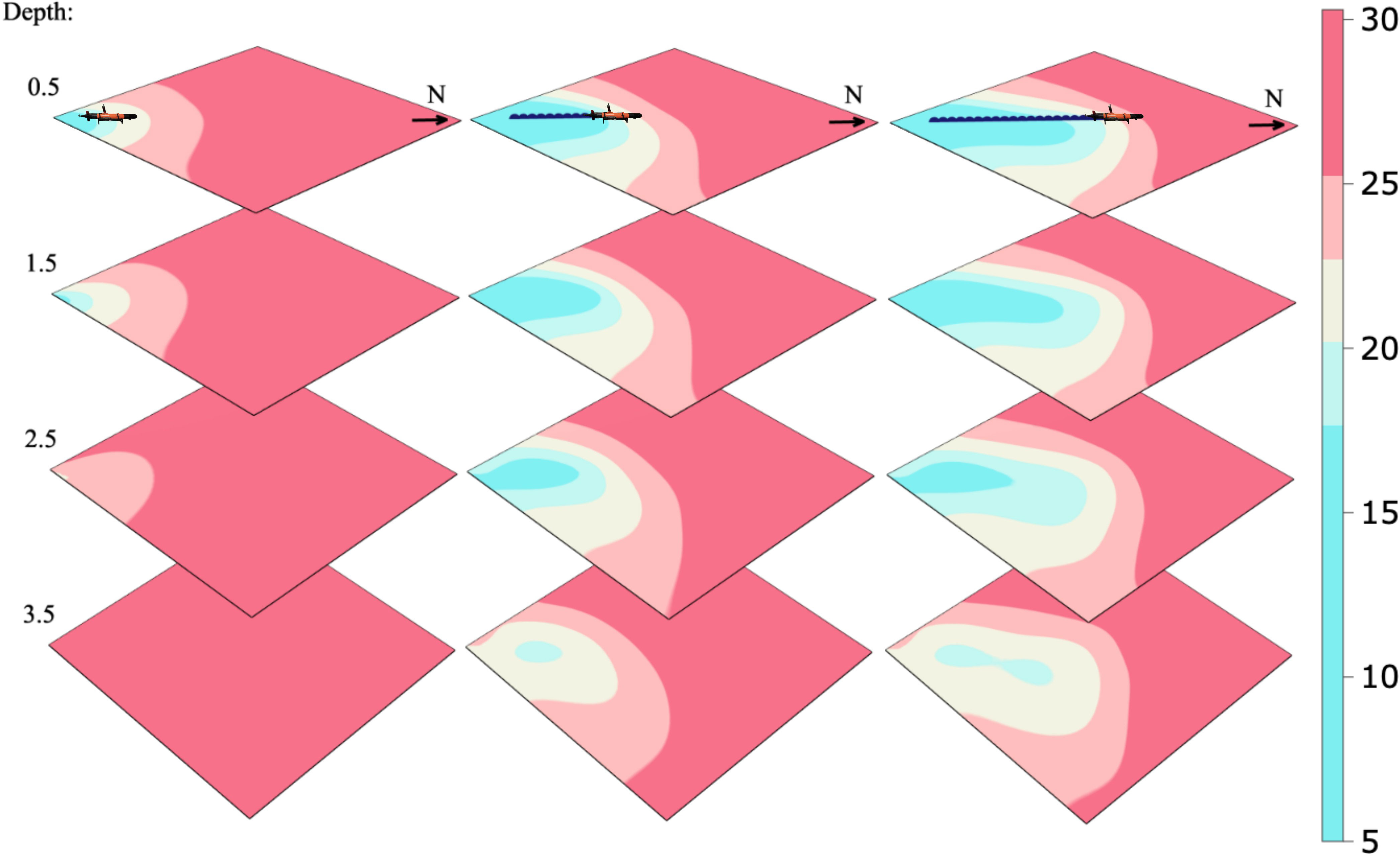
Figure 4 Conditional expectation given AUV measurements along a fixed transect path at a 0.5-m depth.

Figure 5

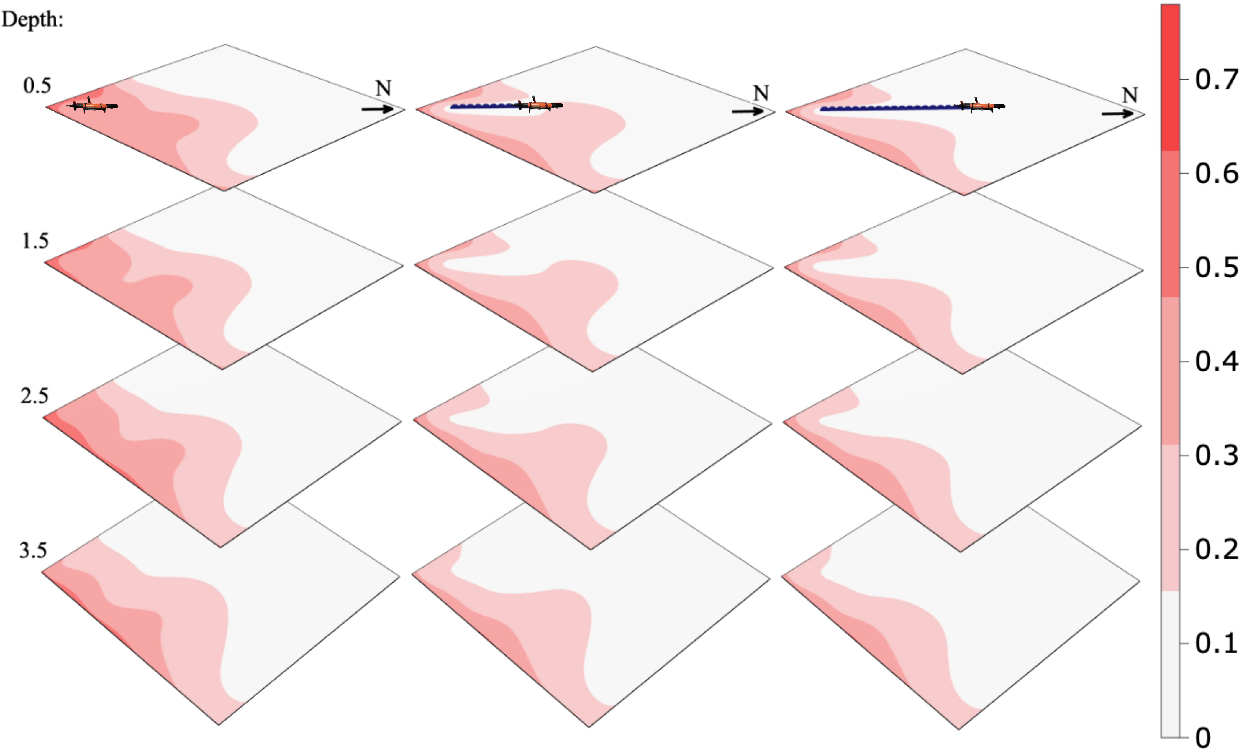
Figure 5 Conditional variance in the process model given AUV measurements along a fixed transect path at a 0.5-m depth.

Figure 6

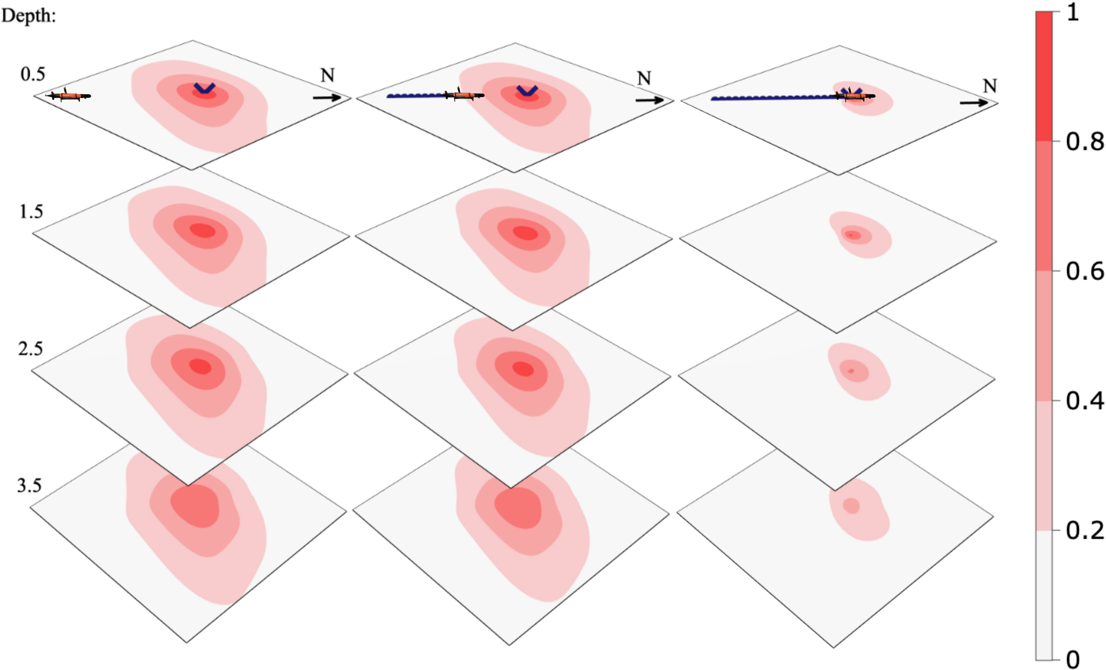
Figure 6 Conditional correlation of the marked point given AUV measurements along a fixed transect path at a 0.5-m depth.

3.2 Excursion sets and plume mapping criterion

One goal of the AUV sampling is to improve the characterization of the plume front defined in our case as the zone separating fresh river waters and more saline fjord waters. Following Fossum et al. (2021) and Ge et al. (2023), we use the uncertainty in the random set of excursions below a salinity threshold ℓ to distinguish river and fjord water. The excursion set is defined by

$$\mathrm{ES}=\{\mathit{s}\in \mathcal{D}:x(\mathit{s})<\ell \}.$$

The associated excursion probability (EP) and the Bernoulli variance (BV) is

$$\mathrm{EP}(\mathit{s})=P(x(\mathit{s})<\ell ), \mathrm{BV}(\mathit{s})=\mathrm{EP}(\mathit{s})[1-\mathrm{EP}(\mathit{s})] s\in \mathcal{D}.$$

The BV is near 0 at locations where the EP is near 0 or 1, whereas it is at its maximum value 0.25 at locations, which have EP equal to 0.5.

When AUV salinity data $\mathit{y}$ are available, we get a conditional GMRF and conditional EPs and BVs. Effective AUV sampling designs get salinity data that can pull these EPs closer to 0 or 1, and in doing so, one reduces the uncertainty of the river plume front. Conditional on salinity data $\mathit{y}={\mathit{y}}_d$ according to design $\mathit{d}\in \mathcal{D}$. The conditional EPs and BVs are

$$P(x(\mathit{s})<\ell |{\mathit{y}}_{\mathit{d}}), P(x(\mathit{s})<\ell |{\mathit{y}}_{\mathit{d}})[1-P(x(\mathit{s})<\ell |{\mathit{y}}_{\mathit{d}})].$$

Design plans must be made before the data${\mathit{y}}_{\mathit{d}}$ is revealed, and we take the expectation over the data when calculating the most effective design. Focusing on improved spatial mapping of the river plume front, it is natural to integrate the objective criterion over all locations in the domain. The expected integrated Bernoulli variance (EIBV) of a design d is then defined by

$\begin{array}{ll}{\text{EIBV}}_d\left(\mathit{\mu },\mathbf{Q}\right)={\displaystyle {\int }_{\mathcal{D}}{E}_{{\mathit{y}}_{\mathit{d}}}\left\{\{P(x(s)<\ell \left|{\mathit{y}}_{\mathit{d}})[1-P(x(s)<\ell \right|{\mathit{y}}_{\mathit{d}})]\}\right\}d\mathit{s}.}& (6)\end{array}$

For the GMRF surrogate model specified by mean µ and precision Q, the EIBV for a design d has a closed form involving sums of bivariate cumulative distribution functions Φ₂ for the Gaussian distribution. In this expression, the design is here involved via a one-entry structure of the selection matrix A = A_d. The closed-form solution facilitates very fast computations of multiple sampling designs. The complete derivations of the closed forms are in the Supplementary Material. See also Fossum et al. (2021) and Ge et al. (2023). In our approach with the sparse GMRF model, we use Monte Carlo sampling from the conditional model to approximate the variance reduction components that are required in the EIBV (see Supplementary Material).

3.3 Adaptive AUV sampling algorithm

The AUV cannot navigate to all possible design locations. Rather, its continued path is constrained by the current location and the possible maneuvers it can perform. We let $\mathcal{P}\subset \mathcal{D}$ denote the possible designs the AUV can choose from, defined by directions (straight, left, right, up, down) from the current AUV location. The chosen design is the one that minimizes the EIBV in Equation (6). This means that

$\begin{array}{ll}{\mathbf{d}}^{\ast }=\mathrm{argma}{\text{x}}_{\mathbf{d}\in \mathcal{P}}\mathrm{EIB}{\text{V}}_d\left(\mathit{\mu },\mathbf{Q}\right).& (7)\end{array}$

During the AUV operation, this kind of design choice is done at many time points, and with an updated model that is conditional on all the data gathered up to this point. In this way, we utilize the benefits of robotic intelligence to navigate the uncertain ocean plume zone.

We outline a myopic adaptive sampling algorithm in the 3D domain. This is a sequential selection of waypoints or grid nodes where the AUV data are sampled and the model updated. The myopic approach represents a heuristic optimization strategy for the AUV operation that does not anticipate potential data or navigation choices beyond the current time. It makes the optimal choice based on the expected values at the current time alone.

Figure 7A shows the idea of adaptive sampling in a sketch with a cycle of tasks where one leads to the next. Here, the AUV senses the salinity, updates its onboard model, and plans where to navigate to, and then it continues on the next cycle.

Figure 7

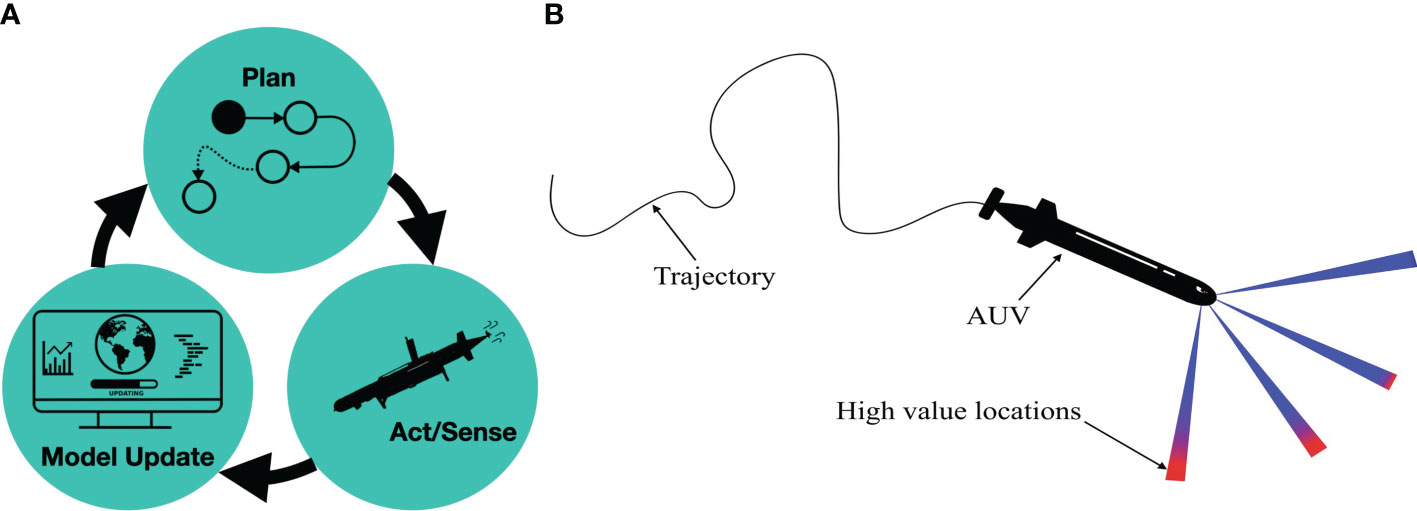
Figure 7 Illustration of the adaptive sampling mechanism. Visualization of the adaptive sampling design (A). The AUV evaluates the potential high-value locations to determine the next visiting waypoint (B). Red colors represent more interesting next waypoints.

Hence, at the planning stage, the computer onboard the AUV solves Equation (7) to navigate in promising 3D directions (Figure 7B). To compensate for the time it takes to do the computation, and to make the system near real time, asynchronous parallel computing is applied to compensate for the excessive computing time onboard.

Algorithm 1 shows the main steps of this adaptive AUV sampling approach. In this algorithm, we use t to indicate subsequent stages of AUV sampling. At stage t, the updated mean in the onboard surrogate model

Algorithm 1. Myopic EIBV minimizing sampling with a GMRF surrogate model.

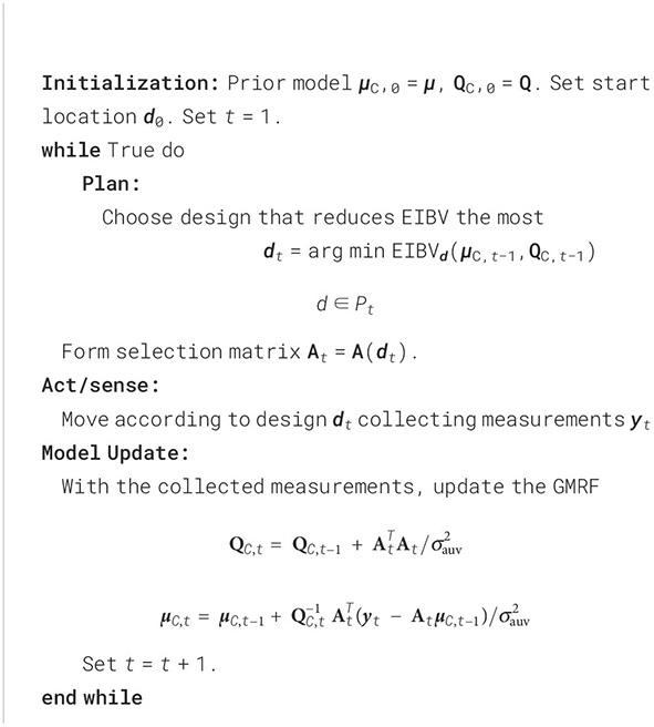
is denoted µ_C,t and the updated precision is Q_C,t. The selection matrix A_t = A(d_t) is formed based on the most promising design d_t at each stage. This design d_t is chosen among several possible designs ${\mathcal{P}}_t\subset \mathcal{D}$ that vary depending on where the AUV is at the current stage and the operational navigation opportunities it has according to the grid. In our implementation, the AUV can continue from its current location to go straight ahead, or turn left, right, up, or down. It cannot return back to its previous grid location (Figure 7B). There are natural exceptions at the grid boundary.

4 Simulation study

In this section, we conduct a simulated experiment to evaluate the performance of our approach for monitoring the three-dimensional freshwater plume of the Nidelva River in Trondheim, Norway. The operational area is outlined in Figure 1. Specifically, we will compare the effectiveness of the suggested complex GRF model and a more standard model. The complex model is discretized with a resolution of 32m x 32m square cells in the horizontal plane and the standard model with a hexagonal grid with a lateral neighbor distance of 120 m. Both models have 1-m-depth increments ranging from 0.5 m to 5.5 m, resulting in a total of n = 50 × 45 × 6 spatial location for the complex model and 1,098 for the standard model. This is in line with the capabilities of the AUVs’ onboard computer.

Initially, both models are estimated on the SINMOD data within the operational area in order to form a prior field. The standard model is specified using a standard variogram analysis, resulting in a Matérn covariance with a lateral correlation range of 550 m, a vertical range of 2 m, a prior marginal variance of 1, and a nugget effect of 0.4 (see Section 2.4 of Cressie (1993) for a description of this spatial data analysis method). The parameters of the complex model are estimated through the approach described in Section 2.3, and detailed in the Supplementary Material and Berild and Fuglstad (2023). Both models use the empirical average across all timesteps (replicates) of the SINMOD data, Equation (3), as its prior expectation.

In order to obtain performance statistics, we ran L = 100 simulated field experiments where the AUV is equipped with either one of the models estimated above and tasked with monitoring the salinity field according to Algorithm 1. The AUV is in this simulation environment exploring a SINMOD dataset from the 09/11/2022 with an assumed additional Gaussian noise term with standard deviation 0.12. This noise represents positional error and measurement error in a real experimental setting. Moreover, the AUV is set to travel at 1 m/s and each simulated field experiment is run for T = 25 sequential steps of Algorithm 1, i.e., visiting 25 spatial locations, where the starting location is kept the same for each run.

Within the lth simulated experiment and after visiting the tth location, the following three metrics are calculated: integrated Bernoulli variance (IBV), root mean squared error (RMSE), and classification error (CE). Let x_l be the ground truth (SINMOD data) in the lth experiment. Then, we calculate the metrics as

$${\text{IBV}}_{l,t}=\sum _{i=1}^n{\text{EP}}_{l,t}({\mathit{s}}_i)\left. [1-{\text{EP}}_{l,t}({\mathit{s}}_i)\right],$$

$${\text{RMSE}}_{l,t}=\sqrt{\frac{1}{n}{\displaystyle \sum _{i=1}^n{[x_l({\mathit{s}}_i)-{\mu }_{C,l,t}({\mathit{s}}_i)]}^2}},$$

$${\text{CE}}_{l,t}=\frac{1}{n}\sum _{i=1}^n\mathbb{I}({\text{E}}_l({\mathit{s}}_i)\ne {\widehat{\text{E}}}_{l,t}({\mathit{s}}_i)), {\text{E}}_l({\mathit{s}}_i)=\mathbb{I}(x_l({\mathit{s}}_i)\le \ell ),{\widehat{\text{E}}}_{l,t}({\mathit{s}}_i)=\mathbb{I}({\mu }_{C,l,t}({\mathit{s}}_i)\le \ell ),$$

where $\mathbb{I}$ is the indicator function, t ∈ [0,T], where T = 25 indicates the sequential step, and $l=1,...,L$ with L = 100 replicate field experiment. The summary statistics of these metrics from the L replicated experiments are shown in Figure 8. The solid lines are the average across all L replicates at time t for each metric, e.g.,

Figure 8

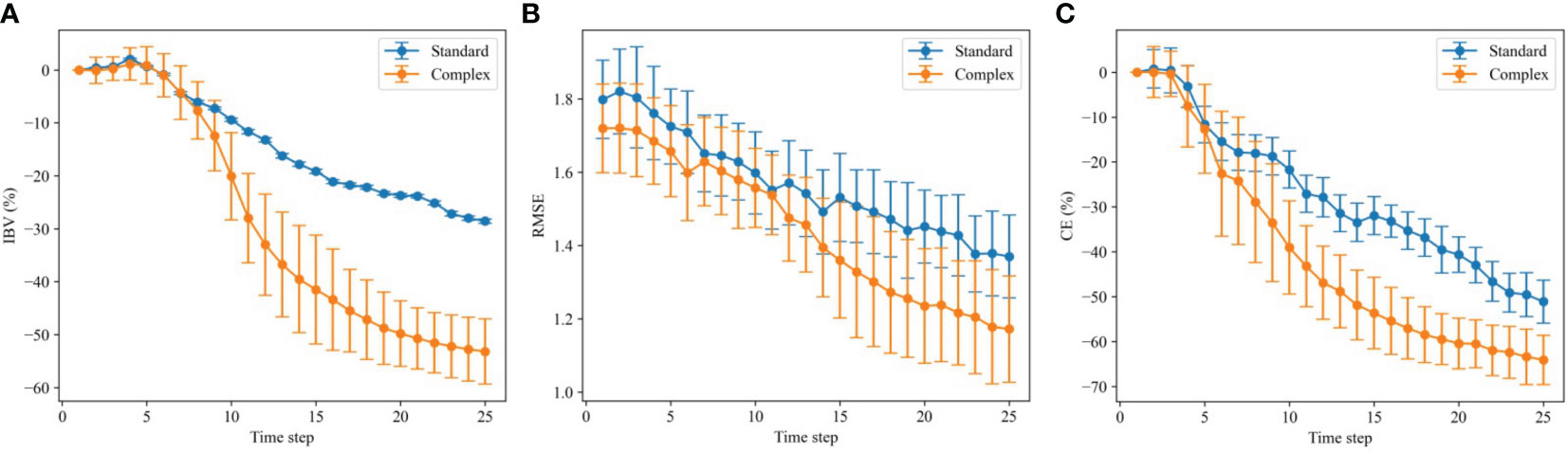
Figure 8 Variation in integrated Bernoulli variance (A), root mean square error (B), and classification error (C) over the 100 replicate runs with the standard model (blue) and the complex model (orange). The solid lines show the averages, and the vertical error bars show the empirical standard deviations of the respective metrics.

$$\widehat{{\text{IBV}}_t}=\frac{1}{L}\sum _{l=1}^L{\text{IBV}}_{l,t},$$

and similarly the error bars show the empirical standard deviation at time t across all L replicates as

$$\mathbb{S}\mathbb{D}\left({\text{IBV}}_t\right)=\sqrt{\frac{1}{L-1}{\displaystyle \sum _{l=1}^L{\left({\text{IBV}}_{l,t}-\widehat{{\text{IBV}}_t}\right)}^2}}.$$

Each display has one of the metrics on the second axis and time stages on the first axis. For the IBV and CE criteria, the percentage reduction compared with the starting value is shown since the models are constructed differently and therefore will also differ prior to the mission, as can be seen in the middle RMSE display.

The IBV reduction (Figure 8A) indicates the ability of the AUV to capture the river plume boundary. A lower IBV means that the AUV is better at sampling the frontal salinity region separating river and fjord water masses. In this spatial example, the IBV has a tendency of going down, even though it could increase at some stages (because data pull probabilities closer to 0.5). The complex GMRF model clearly achieves lower IBV than the simpler model. After some stages, the curve for the complex GMRF model declines rapidly, indicating that the AUV is efficient at exploring the boundary. This means that incorporating a more realistic covariance structure helps the AUV choose the best designs and it tends to move in the right direction.

The RMSE plot (Figure 8B) reflects the similarity between the ground truth and the updated field. The ground truth is here the same as what the AUV is sampling, i.e., the SINMOD dataset from 09/11/2022, but without the added noise term. A lower RMSE means that the AUV is gathering data that helps in predicting the salinity field. Again, the complex model is performing much better than the simpler one. For CE (Figure 8C), a lower value means that the updated model is good at classifying the excursion set associated with the ground truth. The complex model has CE results that are declining faster than the simpler model. The complex model performs better than the standard model due to its versatile capability and flexibility. However, we do realize that training such models often requires expert knowledge and it can be a laborious process to fine-tune the parameters for such a complex model.

In all displays of Figure 8, we observe larger metric variability for the complex GMRF model. The underlying reason for this is the Monte Carlo variance in the EIBV calculation for the GMRF model (see Section 3.2). With the relatively small sampling size, the Monte Carlo error is still not negligible and, influenced by this estimate, the directional sampling decision made by the AUV exhibits more small-scale variability than that of the standard model, which has a closed-form variance expression. Over many replicates, the variability in metrics then gets larger for the GMRF model, especially for the IBV, which relates directly to the AUV sampling decision criterion.

5 Results of Nidelva mission

The field experiment was executed in the Nidelva River plume outside Trondheim, Norway, on the 08/09/2022. The duration of this field deployment spanned 1.5 h. Figure 1 shows the operational area.

5.1 Experimental setup

For this experiment, two AUVs are deployed. This is intended to not only increase the amount of data collected but also enable us to compare the performance of our embedded system under similar conditions. One of the AUVs was programmed with the adaptive sampling algorithm, whereas the other was running with a preprogrammed path plan onboard.

LAUV (Light Autonomous Underwater Vehicle) Harald and LAUV Roald (Figure 9) from the Applied Underwater Robotics Laboratory at NTNU were employed for this mission. LAUV Roald was programmed to carry out the adaptive experiment, and LAUV Harald was programmed to conduct the predesigned plan. To measure the salinity in the water, LAUVs Harald and Roald use CTD sensors, or conductivity, temperature, and depth sensors. Harald uses a SeaBird SBE 49 FastCAT and Roald an AML OEM SV Xchange. Despite being from different manufacturers, the specifications from the suppliers indicate that they should have the same level of precision and accuracy. All the essential scripts were integrated onboard on the backseat NVIDIA Jetson TX2 CPU. For hardware and software in the loop testing and the actual deployment, we relied on the framework developed by Mo-Bjørkelund et al. (2020). The onboard implementation of Algorithm requires Robot Operating Systems (ROS) (Quigley, 2009) and a software bridge to the LAUV, running DUNE (DUNE: Unified Navigation Environment Pinto et al. (2013)) embedded and communicating over the Inter Module Communication (IMC) message protocol (LSTS, 2022).

Figure 9

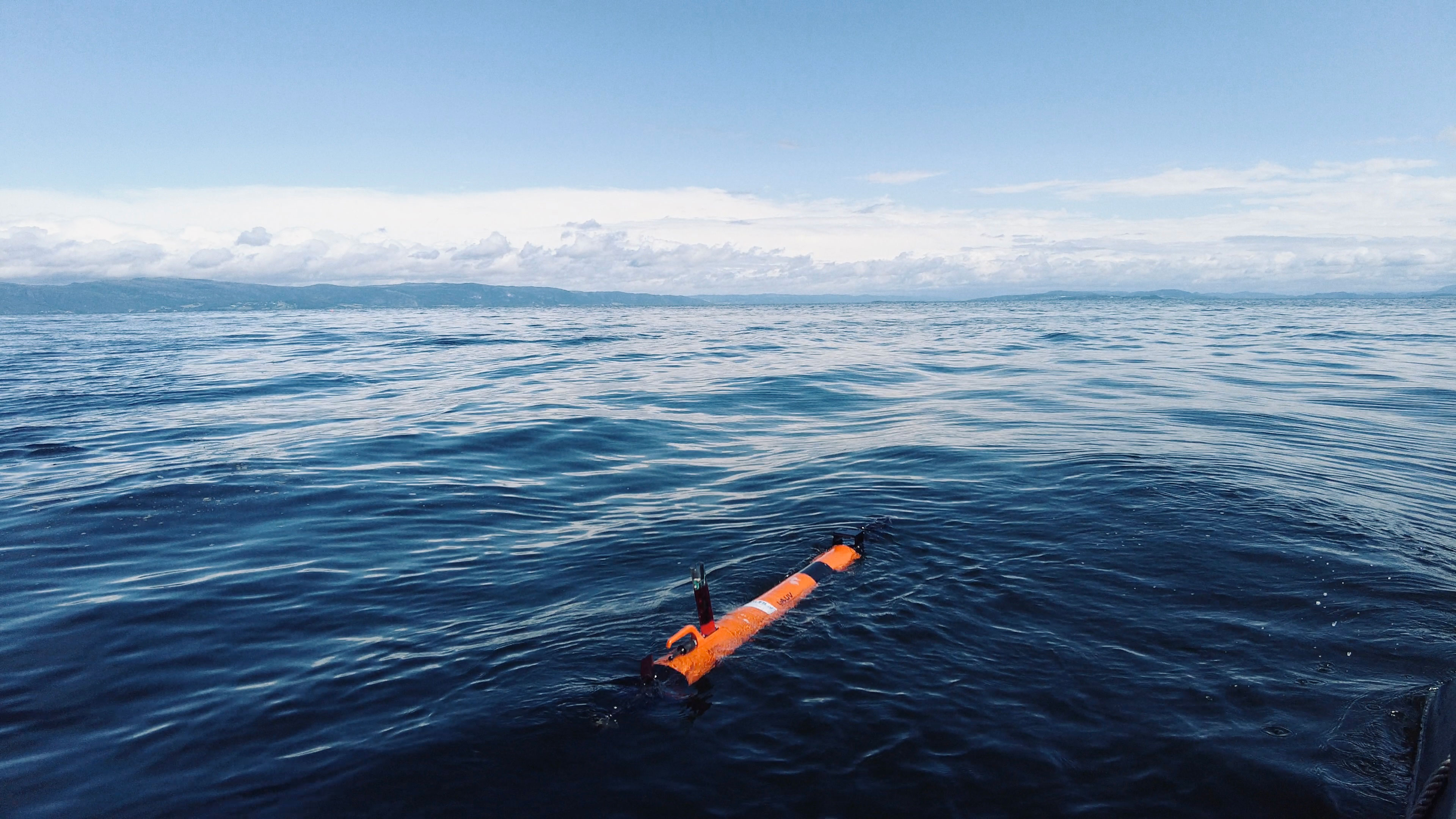
Figure 9 LAUV Roald is on expedition with an adaptive sampling algorithm onboard. The AUV is around 2 m long and runs at around 1 m/s. It is doing a 3D sampling mission at depths ranging from 0.5 m to 5.5 m.

The software bridge between ROS and IMC was adapted from the Swedish Maritime Robotics Centers implementation of a ROS-IMC bridge (Bhat et al., 2020) (https://github.com/smarc-project/imc_ros_bridge) to include messages going from ROS to the vehicle. In addition, a wrapper for the vehicle IMC messages was used, facilitating interaction between the adaptive software and the vehicle. The communication bridge and framework between ROS and IMC use the same back-seat interface as Pinto et al. (2018), with IMC messages being transmitted over Transmission Control Protocol (TCP) (Cerf and Kahn, 1974) between the main CPU and the auxiliary CPU in the AUV. The adaptive code was running on the auxiliary CPU in order to preserve the integrity of the main CPU. For illustration, a flowchart containing the main software components is presented in Figure 10.

Figure 10

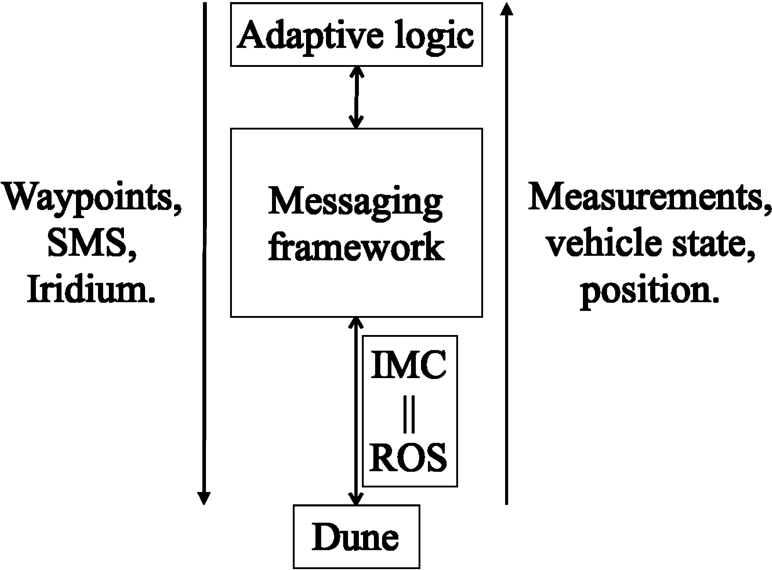
Figure 10 The diagram of the software component in the adaptive sampling system. The main CPU of the AUV is running DUNE (Pinto et al., 2013), whereas IMC (LSTS, 2022) messages are sent through TCP (Cerf and Kahn, 1974) to a secondary CPU, where the adaptive code and ROS (Quigley, 2009) are executed.

Before conducting the principal deployment, we gained understanding of the sea conditions via a preliminary survey. We first launched the pre-survey adaptive mission with a reasonable threshold based on our belief field and then updated the threshold to be 25.4 g/kg after observing the updated salinity field from the pre-survey run.

5.2 Field operation

The AUVs started moving from their starting location around 12:50 a.m. We received the “Mission Complete” message from the AUVs around 14:15 p.m., which marks the end of the operation.

In Figure 11, the results of the AUV conducting adaptive sampling are displayed. Here, we plot the AUV path (black) and the updated posterior mean salinity field over time steps. The AUV began near the river mouth and gradually moved toward the frontal region, occasionally diving to the deeper layers. In total, the AUV traveled approximately 9.734 km, with a coverage of 6.9% of the field at 0.5 m, 6.3% at 1.5 m, 1.6% at 2.5 m, and 0.1% at 3.5m. Both the AUVs were set to travel at 1.5 m/s, but the speed varies widely because of conditions in the ocean. During the mission, the plume expanded due to the tidal effect, so the AUV attempted to follow the front more closely. Interestingly, the AUV did not dive deeper than 2.5 m. This can be attributed to the fact that the water becomes more homogeneous and saline when it is too deep, and the river plume tends to stay close to the upper layers. Also, this can be an effect of the model learning from observation closer to the surface. It should be noted that the trajectory presented in Figure 11 exhibits a seemingly disjointed appearance. This phenomenon arises from the methodology employed, wherein observed measurements are allocated to the nearest center of the grid cell corresponding to their actual spatial location. Furthermore, this disjointedness is exacerbated by the movement of the AUV across various-depth layers, which introduces discontinuities in the trajectories within each layer.

Figure 11

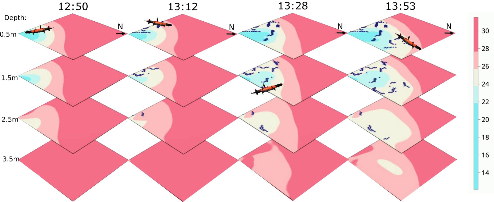
Figure 11 Salinity prediction during the adaptive sampling mission 08/09/2022. The AUV (black) began close to the river mouth and gradually moved toward the frontal region and dived to deeper layers occasionally.

In Figure 12, the salinity prediction results of the AUV’s pre-planned sampling are displayed. The path was designed to maximize the sampling coverage and consequently reduce the variance of the field. The AUV was programmed to move along the path with a consistent YoYo pattern. This pattern involves the AUV moving between 0.5 m and 5.5 m repeatedly. The preprogrammed path approach ensures a more systematic and exhaustive coverage of the volume, providing a broader perspective but lacking the pinpoint accuracy on such a large and rapidly changing ocean volume. The path the AUV traveled along was approximately 9.346 km with a coverage of 7.9% at 0.5 m, 8.3% at 1.5 m, 9.1% at 2.5 m, 8.6% at 3.5 m, 7.9% at 4.5 m, and 7.2% at 5.5 m.

Figure 12

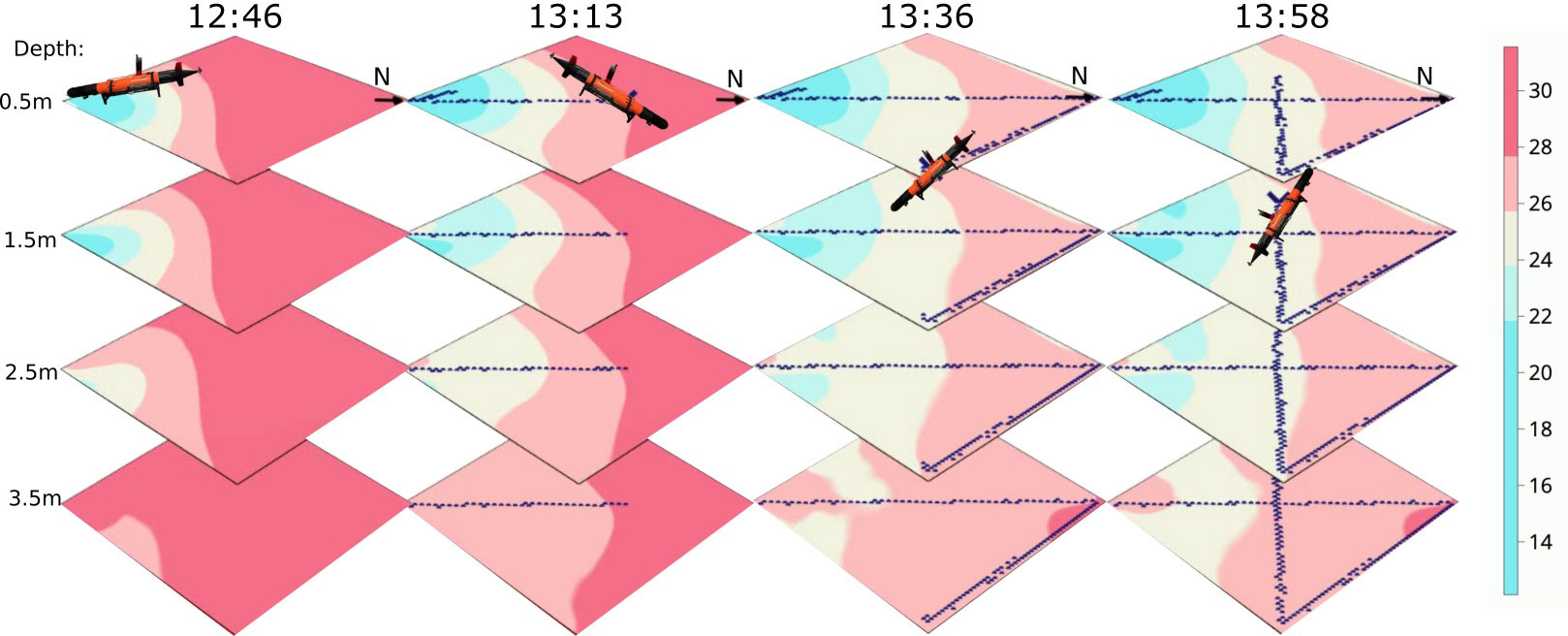
Figure 12 Salinity prediction during the fixed path mission on 08/09/2022. The AUV (black) aims to cover the spatial domain.

Given the unpredictable nature of the location of the freshwater front, it is virtually impossible to preplan precise sampling paths. The shifts and movements of the plume demand a real-time responsive approach like adaptive sampling. This is also evident when comparing Figures 11, 12. On the other hand, if a broad overview of the ocean volume is the goal, then a preplanned design likely is useful to ensure a systematic coverage of the region, leaving minimal gaps in the data collection. Also, note that diving 1 m is significantly more time efficient than moving 32 m in the horizontal plane for the AUV, this can be viewed by the coverage in each layer by two missions. The fixed path mission has good coverage within each layer whereas the adaptive mission mostly considers the top two layers. Because of this, it could be interesting in future work to consider adaptive sampling in only the horizontal plane and to always move in a YoYo pattern.

5.3 SINMOD and AUV data comparison

Even though salinity is only one state variable in SINMOD, it is useful and interesting to compare the AUV salinity measurements with the predictions made by SINMOD, as it will give information on the overall performance of the hydrodynamic model. Using all the data collecting by both AUVs, we compare the location-specific observations made by the AUVs with the associated SINMOD predictions for this day.

As illustrated in Figure 13, there is a clear inclination of SINMOD to overpredict salinity values. This trend is evident as a majority of the AUV measurements are situated below the zero error line (dotted line). In shallow water regions, both SINMOD and the AUV measurements exhibited high salinity variability, which is reasonable considering the freshwater influx from the river and local disturbances. For deeper waters, the salinity is higher for both models and more concentrated, with a bias around 3.5 g/kg between the SINMOD predictions and AUV measurements. The highest measured salinity value by the AUV was 28.0 g/kg, whereas the highest value from SINMOD was 31.5 g/kg, further confirming that the numerical model overestimates salinity both for the water in the river plume and in the brackish layer in the fjord.

Figure 13

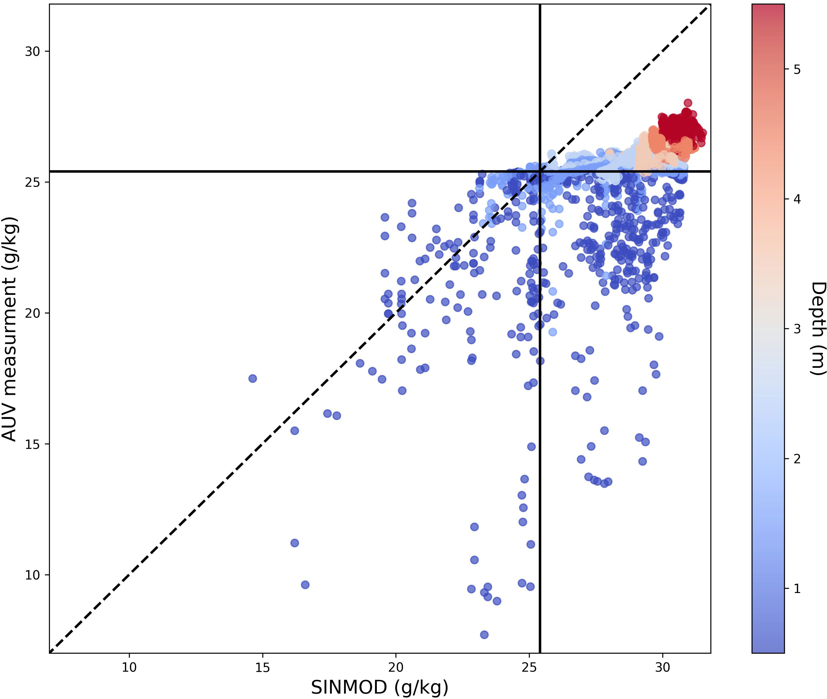
Figure 13 Comparison of salinity values estimated from the numerical ocean model (x-axis) and salinity measurements collected with the AUV on the 8th of September 2022 (y-axis) where the color shows the corresponding depths. The dotted line shows the zero error line.

While this discrepancy between SINMOD and the actual salinity field is evident, this will not impact the learning of the covariance structure, which captures the spatial correlation and variability within the data and is independent of any systematic bias. That said, the observed overestimation in SINMOD does set a prior expectation in our model that is skewed slightly high and will initially impact the adaptive sampling algorithm.

6 Conclusions

In this study, we have presented an approach for effective 3D (north, east, depth) sampling of salinity in a river plume front, employing a realistic and flexible spatial covariance model running onboard an AUV in real time. Results of a deployment in the Trondheim fjord demonstrate that prior inputs from the SINMOD numerical ocean model are effectively calibrated with the in-situ AUV measurements. In a mission focusing on mapping the frontal region, the AUV adapts naturally to the updated situation and zig-zags near the plume front to improve its spatial characteristics. Moreover, it is evident that the adaptive approach holds a distinct advantage over the preplanned method when it comes to accurately monitoring dynamic zones like the river plume front.

In Section 2.3, we estimate our surrogate model with the prior mean and covariance structure, which in the visualization both appear reasonable and are well-suited for the domain of interest. Furthermore, as detailed in Section 4, the surrogate model consistently outperformed a standard benchmark model across several key performance metrics. Lastly, in Section 5.2, we present the results of the field mission. Figure 11 depicts the AUV’s predictions throughout the adaptive sampling mission, which we interpret as indicative of reasonable adaptive sampling behavior under the given conditions. The surrogate model, while promising in these results, does necessitate further refinement to fully realize its potential in this context. Firstly, refining its parameterization slightly to simplify the likelihood surface can potentially improve the optimization process significantly. Furthermore, estimating the covariance structure to innovations constructed from the SINMOD data, as described in Berild and Fuglstad (2023), is not guaranteed to be accurate in removing the temporal effect in the data, thus making it challenging to ascertain if the final structure is only capturing the spatial effect.

The prior models used in this work included 3D space with no temporal variation. A natural extension is to include temporal variation in the prior, which could be done in a Gaussian framework assuming known advection and diffusion (Foss et al., 2022). However, more research is required to develop realistic space–time models for frontal regions, such as that associated with river plumes, while maintaining the computational efficiency required to conduct expansive field surveying as considered in this study. Lastly, our exploration was confined to a near-sighted myopic sampling scheme. Future avenues might explore more sophisticated strategies (Bai et al., 2021), using longer sampling horizons where one can look ahead and anticipate the information gained by traversing longer distances with the AUV while also accounting for operational constraints.

In closing, it is important to highlight that while our study is centered on separating ocean masses of low (freshwater plume) and high (brackish water) salinity concentrations, we believe that this approach transfers well to other applications in physical or biological oceanography, such as polar melting water, high chlorophyll concentrations, oxygen or carbon content, or pollution detection.

Data availability statement

The datasets presented in this study can be found in online repositories. The names of the repository/repositories and accession number(s) can be found below: https://doi.org/10.17605/OSF.IO/RHDKM.

Author contributions

MB: Methodology, Software, Writing – original draft, Data curation, Formal analysis. YG: Methodology, Software, Writing – original draft, Data curation, Formal analysis. JE: Conceptualization, Methodology, Project administration, Supervision, Writing – review & editing. G-AF: Conceptualization, Methodology, Supervision, Writing – review & editing. IE: Data curation, Writing – review & editing.

Funding

The author(s) declare financial support was received for the research, authorship, and/or publication of this article. This work is funded by the Norwegian Research Council through the MASCOT project 305445.

Acknowledgments

We acknowledge the aid and support of AURlab (https://www.ntnu.edu/aur-lab) in lending us the AUVs and help in running multiple field mission.

Conflict of interest

The authors declare that the research was conducted in the absence of any commercial or financial relationships that could be construed as a potential conflict of interest.

Publisher’s note

All claims expressed in this article are solely those of the authors and do not necessarily represent those of their affiliated organizations, or those of the publisher, the editors and the reviewers. Any product that may be evaluated in this article, or claim that may be made by its manufacturer, is not guaranteed or endorsed by the publisher.

Supplementary material

The Supplementary Material for this article can be found online at: https://www.frontiersin.org/articles/10.3389/fmars.2023.1319719/full#supplementary-material

References

Bai S., Shan T., Chen F., Liu L., Englot B. (2021). Information-driven path planning. Curr. Robotics Rep. 2, 177–188. doi: 10.1007/s43154-021-00045-6

CrossRef Full Text | Google Scholar

Beldring S., Engeland K., Roald L. A., Sælthun N. R., Voksø A. (2003). Estimation of parameters in a distributed precipitation-runoff model for Norway. Hydrology Earth System Sci. 7, 304–316. doi: 10.5194/hess-7-304-2003

CrossRef Full Text | Google Scholar

Berget G. E., Eidsvik J., Alver M. O., Johansen T. A. (2023). Dynamic stochastic modeling for adaptive sampling of environmental variables using an auv. Autonomous Robots 47, 483–502.

Google Scholar

Berget G. E., Fossum T. O., Johansen T. A., Eidsvik J., Rajan K. (2018). Adaptive sampling of ocean processes using an auv with a gaussian proxy model. IFAC-PapersOnLine 51, 238–243.

Google Scholar

Berild M. O., Fuglstad G.-A. (2023). Spatially varying anisotropy for gaussian random fields in three-dimensional space. Spatial Stat 55, 100750.

Google Scholar

Bhat S., Torroba I., Özkahraman Ö., Bore N., Sprague C. I., Xie Y., et al. (2020). “A cyber-physical system for hydrobatic auvs: system integration and field demonstration,” in 2020 IEEE/OES Autonomous Underwater Vehicles Symposium (AUV). 1–8 (St. Johns, NL, Canada: IEEE).

Google Scholar

Broch O. J., Daae R. L., Ellingsen I. H., Nepstad R., Bendiksen E.Å., Reed J. L., et al. (2017). Spatiotemporal dispersal and deposition of fish farm wastes: a model study from central Norway. Front. Mar. Sci. 4, 199.

Google Scholar

Broch O. J., Klebert P., Michelsen F. A., Alver M. O. (2020). Multiscale modelling of cage effects on the transport of effluents from open aquaculture systems. PloS One 15, e0228502.

PubMed Abstract | Google Scholar

Cerf V., Kahn R. (1974). A protocol for packet network intercommunication. IEEE Trans. Commun. 22, 637–648. doi: 10.1109/TCOM.1974.1092259

CrossRef Full Text | Google Scholar

Cressie N. (1993). Statistics for spatial data (New York: John Wiley & Sons).

Google Scholar

Das J., Py F., Harvey J. B., Ryan J. P., Gellene A., Graham R., et al. (2015). Data-driven robotic sampling for marine ecosystem monitoring. Int. J. Robotics Res. 34, 1435–1452.

Google Scholar

Doney S. C., Ruckelshaus M., Emmett Duffy J., Barry J. P., Chan F., English C. A., et al. (2012). Climate change impacts on marine ecosystems. Annu. Rev. Mar. Sci. 4, 11–37. doi: 10.1146/annurev-marine-041911-111611

CrossRef Full Text | Google Scholar

Fonseca J., Bhat S., Lock M., Stenius I., Johansson K. H. (2023). Adaptive sampling of algal blooms using autonomous underwater vehicle and satellite imagery: Experimental validation in the baltic sea, arXiv preprint arXiv:2305.00774.

Google Scholar

Foss K. H., Berget G. E., Eidsvik J. (2022). Using an autonomous underwater vehicle with onboard stochastic advection-diffusion models to map excursion sets of environmental variables. Environmetrics 33, e2702.

Google Scholar

Fossum T. O., Eidsvik J., Ellingsen I., Alver M. O., Fragoso G. M., Johnsen G., et al. (2018). Information-driven robotic sampling in the coastal ocean. J. Field Robotics 35, 1101–1121. doi: 10.1002/rob.21805

CrossRef Full Text | Google Scholar

Fossum T. O., Fragoso G. M., Davies E. J., Ullgren J. E., Mendes R., Johnsen G., et al. (2019). Toward adaptive robotic sampling of phytoplankton in the coastal ocean. Sci. Robotics 4, eaav3041. doi: 10.1126/scirobotics.aav3041

CrossRef Full Text | Google Scholar

Fossum T. O., Travelletti C., Eidsvik J., Ginsbourger D., Rajan K. (2021). Learning excursion sets of vector-valued Gaussian random fields for autonomous ocean sampling. Ann. Appl. Stat 15, 597–618. doi: 10.1214/21-AOAS1451

CrossRef Full Text | Google Scholar

Fuglstad G.-A., Lindgren F., Simpson D., Rue H. (2015). Exploring a new class of non-stationary spatial gaussian random fields with varying local anisotropy. Statistica Sin. 25, 115–133.

Google Scholar

Ge Y., Eidsvik J., Mo-Bjørkelund T. (2023). 3d adaptive auv sampling for classification of water masses. IEEE J. Ocean Eng. 48, 626–639.

Google Scholar

Gramacy R. B. (2020). Surrogates: Gaussian process modeling, design, and optimization for the applied sciences (New York: CRC press).

Google Scholar

Halpern B. S., Walbridge S., Selkoe K. A., Kappel C. V., Micheli F., D’Agrosa C., et al. (2008). A global map of human impact on marine ecosystems. Science 319, 948–952. doi: 10.1126/science.1149345

PubMed Abstract | CrossRef Full Text | Google Scholar

Hoegh-Guldberg O., Bruno J. F. (2010). The impact of climate change on the world’s marine ecosystems. Science 328, 1523–1528. doi: 10.1126/science.1189930

PubMed Abstract | CrossRef Full Text | Google Scholar

Lindgren F., Rue H., Lindström J. (2011). An explicit link between Gaussian fields and Gaussian Markov random fields: the stochastic partial differential equation approach. J. R. Stat. Society: Ser. B (Statistical Methodology) 73, 423–498.

Google Scholar

Lin M., Yang C. (2020). Ocean observation technologies: A review. Chin. J. Mechanical Eng. 33, 32. doi: 10.1186/s10033-020-00449-z

CrossRef Full Text | Google Scholar

LSTS (2022) Inter module communication protocal. Available at: https://lsts.pt/docs/imc/master (Accessed Accessed: 2022-11-01). Dataset.

Google Scholar

Mo-Bjørkelund T., Fossum T. O., Norgren P., Ludvigsen M. (2020). “Hexagonal grid graph as a basis for adaptive sampling of ocean gradients using AUVs,” in Global Oceans 2020. 1–5 (Singapore: U.S. Gulf Coast), ISBN: ISSN: 0197-7385. doi: 10.1109/IEEECONF38699.2020.9389324

CrossRef Full Text | Google Scholar

Nepstad R., Liste M., Alver M. O., Nordam T., Davies E., Glette T. (2020). High-resolution numerical modelling of a marine mine tailings discharge in western Norway. Regional Stud. Mar. Sci. 39, 101404.

Google Scholar

Nepstad R., Nordam T., Ellingsen I. H., Eisenhauer L., Litzler E., Kotzakoulakis K. (2022). Impact of flow field resolution on produced water transport in lagrangian and eulerian models. Mar. pollut. Bull. 182, 113928.

PubMed Abstract | Google Scholar

Pinto J., Dias P. S., Martins R., Fortuna J., Marques E., Sousa J. (2013). “The lsts toolchain for networked vehicle systems,” in 2013 MTS/IEEE OCEANS - Bergen. 1–9. doi: 10.1109/OCEANS-Bergen.2013.6608148

CrossRef Full Text | Google Scholar

Pinto J., Mendes R., da Silva J. C. B., Dias J. M., de Sousa J. B. (2018). “Multiple autonomous vehicles applied to plume detection and tracking,” in 2018 OCEANS - MTS/IEEE Kobe Techno-Oceans (OTO). 1–6. doi: 10.1109/OCEANSKOBE.2018.8558802

CrossRef Full Text | Google Scholar

Quigley M., Gerkey B., Conley K., Faust J., Foote T., Leibs J. (2009). ROS: an open-source Robot Operating System. ICRA workshop on open source software. 3, 5. Kobe, Japan.

Google Scholar

Slagstad D., McClimans T. A. (2005). Modeling the ecosystem dynamics of the Barents sea including the marginal ice zone: I. Physical and chemical oceanography. J. Mar. Syst. 58, 1–18. doi: 10.1016/j.jmarsys.2005.05.005

CrossRef Full Text | Google Scholar

Slagstad D., Wassmann P. F., Ellingsen I. (2015). Physical constrains and productivity in the future arctic ocean. Front. Mar. Sci. 2, 85.

Google Scholar

Vernet M., Ellingsen I., Marchese C., Bélanger S., Cape M., Slagstad D., et al. (2021). Spatial variability in rates of net primary production (npp) and onset of the spring bloom in Greenland shelf waters. Prog. Oceanography 198, 102655.

Google Scholar

Zhang Y., Bellingham J. G., Ryan J. P., Kieft B., Stanway M. J. (2013). “Two-dimensional mapping and tracking of a coastal upwelling front by an autonomous underwater vehicle,” in 2013 OCEANS - San Diego. 1–4, ISBN: ISSN: 0197-7385. doi: 10.23919/OCEANS.2013.6741231

CrossRef Full Text | Google Scholar

Zhang Y., Ryan J. P., Bellingham J. G., Harvey J. B. J., McEwen R. S. (2012). Autonomous detection and sampling of water types and fronts in a coastal upwelling system by an autonomous underwater vehicle. Limnology Oceanog: Methods 10, 934–951. doi: 10.4319/lom.2012.10.934

CrossRef Full Text | Google Scholar