 Yaowei Ma
 Qinghong Li*
- Department of Military OceanGraphy and Hydrography, Dalian Naval Academy, Dalian, China
Mesoscale eddies are omnipresent and play an important role in regulating Earth’s climate and ocean circulation in the global ocean. Here using the combination of satellite altimetry products and Argo float profile data, two types of abnormal eddies are investigated: WCEs(warm cyclonic eddies) and CAEs(cold anticyclonic eddies) with different cores than conventional eddies in the Japan/East Sea. By applying a classification method based on the calculation of the heat content anomalies in the upper ocean, it was found that 10% of the eddies that captured the Argo float profiles exhibited obvious abnormal features. Subsequently, their spatiotemporal distributions and characteristics were analyzed statistically. Three-dimensional structures of abnormal eddies were obtained via the composite analysis method, showing that the warm/cold and light/dense core of the composite WCE/CAE is confined to the upper 100 m of the ocean with a maximum temperature anomaly of approximately +1.0(-1.1)°C. The composite WCE had a double-core salinity structure with a salty core above 50 m and an inferior fresh core. Meanwhile composite CAE had a fresh single-core with a maximum magnitude of -0.05 psu. Abnormal eddies are pervasive in the Japan/East sea, a revaluation of the role of these eddies in ocean circulation and climate systems, such as heat and salt transport, air and sea interaction, and variability in mixed layer depth, is of great importance.
1 Introduction
Mesoscale eddies, which are commonly present as self-sustaining localized vortexes, act as disseminators of oceanic mass(Zhang et al., 2014), thus regulating the distribution of heat, salt, chlorophylls, dissolved carbon, and other tracers (Kahru et al., 2007; Chelton et al., 2011a; Dong et al., 2014; Nagai et al., 2015; Wang et al., 2018). Mesoscale kinetic energy dominate approximately 90% of the kinetic energy in the global ocean (Pascual et al., 2006; Chelton et al., 2011b). These mesoscale eddies play an important role in ocean–atmosphere circulation by modulating the Earth’s climate and marine environment (Frenger et al., 2013; Yan et al., 2022; Seo et al., 2023). In addition, mesoscale eddies can change oceanographic physical parameters, such as the depths of upper mixed layers, which trigger vertical water exchange and affect the biological productivity of marine ecosystems (Siegel et al., 2011; Itoh et al., 2021; Liu et al., 2023).
Based on sea level anomalies and the direction of rotation, mesoscale eddies can be classified into anticyclonic eddies (AEs), with a lifted sea surface height and cyclonic eddies (CEs), with a depressed sea surface height. Therefore, over the past few years, satellite altimetry products have often been used to detect eddies in global oceans (Chelton et al., 2011b; Faghmous et al., 2015). To investigate the three-dimensional structure of eddies, satellite products are often combined with in-situ measurements, such as Argo float to acquire subsurface information (Chaigneau et al., 2011; Yang et al., 2013; Zhang et al., 2013; Yang et al., 2015; Amores et al., 2016; Zhang et al., 2018; He et al., 2021).
From a conventional perspective, AEs/CEs are often associated with a warmer/colder cores in comparison to that of the background water mass. Nevertheless, recent studies have identified numerous abnormal eddies with opposite-temperature structures, including AEs with cold cores and CEs with warm cores (Itoh and Yasuda, 2010; Liu et al., 2021; Ni et al., 2021; An et al., 2022; Qi et al., 2022; Sun et al., 2023). In this study, these eddies are respectively named cold-core anticyclonic eddies (CAEs) and warm-core cyclonic eddies (WCEs). In contrast, conventional eddies are referred to as warm-core anticyclonic eddies (WAEs) and cold-core cyclonic eddies (CCEs).
Numerous studies have reported cases of abnormal eddies in different regions of the global ocean. Cold anticyclonic eddies in the western boundary region of the subarctic northern Pacific were discovered using a combination of satellite altimetry and multi-source vertical profile data, and were mainly found around the Oyashio southward intrusion with cold and fresh core water (Itoh and Yasuda, 2010). The global distribution of the abnormal eddies(WCEs and CAEs) was presented by Ni et al. (2021) along with their composite vertical structures and influence on the marine environment. Liu et al. (2021) developed a framework based on deep learning to mine global satellite information from sea surface height (SSH) and sea surface temperature (SST) data. The authors determined that abnormal eddies account for approximately one-third of total eddies, which is an astonishing discovery. An abnormal anticyclonic eddy surface, characterized by a lens-shaped structure and a cold core, was investigated by 3-day in-situ observations in the northern South China Sea (SCS), the conductivity-temperature-depth(CTD) and acoustic doppler current profiler(ADCP) measurements produced comprehensive information about the eddy’s characteristics (Qi et al., 2022). Using eddy-resolving model data (OFES) from 2008 to 2017, a considerable amount of abnormal eddies were found to exist in the Kuroshio-Oyashio extension region and North Pacific Subtropical Countercurrent (STCC) region, and their spatial and seasonal variations have been exhaustively investigated (An et al., 2022; Sun et al., 2023). Although their definitions and detection methods of abnormal eddies are different, it can be confirmed that abnormal mesoscale eddies are ubiquitous in the global ocean. Consequently, an investigation into the spatiotemporal distribution and vertical structure of the upper ocean will be of vital importance to re-evaluate the effects on air-sea exchanges and ocean thermohaline circulation caused by mesoscale eddies in various oceanic regions. Because abnormal eddies have three-dimensional structures, satellite data alone cannot reflect their comprehensive information, therefore in-situ observational data, such as Argo profiles, are crucial additions.
As the largest marginal sea in the Northwestern Pacific Ocean, Japan/East Sea is connected to open seas by the Soya, Tatar, Tsushima, and Tsugaru Strait, it also has a cyclonic oceanic circulation inside its basin (Figure 1), which is an activate region for mesoscale eddies’ formation and evolution (Jacobs et al., 1999; Morimoto et al., 2000; Lee and Niiler, 2010). Its western margin is located in the Russian Far East area and Korean Peninsula, and the eastern boundary is located west of the Japanese Archipelago and southwest of Sakhalin Island. In a previous study, a CAE was discovered in the southern Sea of Japan (Hosoda and Hanawa, 2004). However, limited information is available on abnormal eddies in the Japan Basin, particularly their vertical structures. The estimation of the effect of abnormal eddies on physical parameters such as mixed layer depth variation and eddy heat flux in the Japan/East Sea is unknown. Therefore, a detailed investigation into the spatiotemporal distribution and vertical structure in the upper ocean is of vital importance to re-evaluate the effects on air-sea exchanges and ocean thermohaline circulation caused by mesoscale eddies in different oceanic regions.
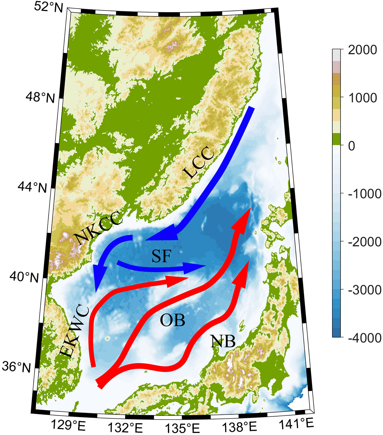
Figure 1 The schematic surface circulation distribution of the Japan/East Sea. Blue and Red) arrows denote cold and warm currents, respectively. LCC: Liman Cold Current; NKCC, North Korea Cold Current; EKWC, East Korea Warm Current; SF, Subpolar Front; OB, offshore branch; NB, Nearshore branch; TWC, Tsushima Warm Current (a branch of the Kuroshio, the main input current of Japan/East sea). Background topography and bathymetry is collected from ETOPO1 dataset with a 1 arc-minute resolution.
The remainder of this study is organized as follows: The satellite altimetry and Argo data used in this study and the classification criteria for dividing mesoscale eddies into four categories(WAEs, CAEs, CCEs, WCEs) according to heat/salt content anomalies, which are introduced in Section 2. The analysis of spatioltemporal statistical characteristics of the different types of eddies are presented in Section 3. The composite vertical temperature, salinity, and potential density anomaly fields from the combination of the satellite altimeter and Argo float profile, especially the three-dimensional structure of the abnormal eddies, are presented in Section 4. Finally, section 5 presents the conclusions of this study.
2 Materials and methods
2.1 Altimetry data and mesoscale eddy data set
A daily sea surface anomaly (SLA) atlas with a spatial resolution of 0.25° ×0.25° provided by Archiving, Validation, and Interpretation of Satellite Oceanographic (AVISO; https://www.aviso.altimetry.fr/) was used in this study to identify mesoscale eddies in Japan/East Sea. This multi-mission gridded satellite altimeter product merged measurements from more than two satellite altimeters, such as T/P-Jason, ERS-1, ERS-2 and others (Ducet et al., 2000) from January 2011 to December 2021. Here, we adopted the SLA-based autonomous eddy identification algorithm proposed by Faghmous et al. (2015), which can provide trajectories, amplitudes, contours, and other features of global eddies. Before using the identification algorithm, the SLA data was high-passed filtered with a 180-day cutoff filter to remove large-scale circulation signals. The META3.2exp mesoscale eddy trajectory atlas derived from AVISO altimetry product (Pegliasco et al., 2022) was also adopted in this study for comparative reference. This dataset incorporates the polarity, location, amplitude, radius, boundary, and movement trajectories of eddies. We selected only eddies with lifespans longer than 14 d to ensure the reliability of the subsequent composite results. Finally, we identified 1114 and 1776 AE and CE trajectories with 51975 and 59802 snapshots, respectively, in the Japan/East Sea from 2011 to 2021.
The eddy radius was calculated as , where A is the effective area enclosed by an effective eddy contour. Eddy amplitude is defined as the absolute value of the height difference between the extremum of SLA within the eddy and the mean SLA around the effective contour, namely, the eddy edge used in the preceding eddy radius estimation.
2.2 Argo profile data
The delayed-mode Argo float profile obtained from IFREMER (https://data-argo.ifremer.fr) was used to gain more information based on the subsurface of the eddies. However, before conducting further research, a quality control (QC) procedure was applied to these unprocessed Argo datasets. Only profile data satisfying the following conditions were selected: (1) the quality flag of the pressure, temperature, and salinity data must be 1 or 2, from a rating of 0-3, with 0 being the lowest quality. (2) The QC indices of the time and position of the profile must be 1. (3) The shallowest measurement point should be above 10 m in depth and the deepest data should be below 800 m. (4) The number of data levels in the profile should exceed 25, and the depth difference between two adjacent levels should be less than 25 m for the 0-300 m level and less than 50 m for 300-800 m level.
Once the filter criteria were adhered to, 11730 profiles of the T/S anomaly remained. The Argo profiles were then matched to the eddies detected in the Japan/East Sea. For each eddy snapshot, the simultaneous Argo float capture (the eddy encompassed at least one Argo profile inside its boundary) was selected and each profile was visually checked to ensure that the T/S anomaly data were reliable. Finally, we adopted 7275 profiles in total, including 3405 and 3870 profiles captured by cyclonic and anticyclonic eddies, respectively, accounting for approximately 62% of the initial Argo profile dataset, their spatiotemporal distribution is shown in Figure 2A. As shown in Figure 2B, the overall number of Argo profiles presented a continuously decreasing trend from 2012 to 2016. Subsequently, the number increased in 2017, temporarily dipped in 2018 and surged during the summer of 2019. Then, the Argo profile number plunged to zero from August 2020 to March 2021 and increased again in the remaining months of 2021. An average of 30 Argo profiles were captured by mesoscale eddies each month, ensuring sufficient material for the subsequent composite analysis. The derived quantities, such as the potential density and mixed layer depth, were then calculated from the gridded T/S profile.
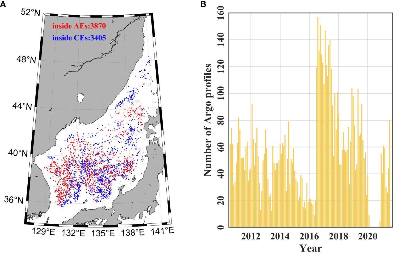
Figure 2 Spatiotemporal distribution of Argo profiles captured by mesoscale eddies in the Japan/East Sea from 2011 to 2021. (A) The positions of 7275 Argo float profiles, thereinto 3870 profiles surfacing into AEs (red) and 3405 profiles surfacing into CEs (blue). (B) Monthly variations of the number of Argo float profiles from 2011 to 2021. AE, anticyclonic eddies; CE, cyclonic eddies.
2.3 Composite method
In this study, we used a composite analysis method to reveal the vertical structures of the temperature, salinity, and potential density anomalies of abnormal and normal eddies. The key concept of the composite analysis is to project plentiful Argo float profiles (captured by different desynchronous eddies) into a coordinated system with the eddy center as the origin to form a statistically averaged three-dimensional structure of mesoscale eddies in a selected research region. The specific procedures are as follows: (1) Maintain a record of every Argo float profile in the Japan/East Sea from 2011 to 2021, and if individual profiles are captured in an eddy (defined as being located in the eddy), we matched this eddy snapshot with one or more captured Argo profiles. (2) Once matching was complete, all Argo profiles were projected into the eddy-center coordinate system (ΔX, ΔY); to eliminate the effect of the variability of different eddy sizes, we used the eddy’s radius to divide the distance from Argo to eddy center, and obtain the normalized coordinates (Δx, Δy), with Δx = ΔX/R, Δy = ΔY/R, where R is the radius of the eddy. (3) Finally, all profiles in this coordinate system were objectively mapped onto a 0.1×0.1 grid using divand 1.0 (Barth et al., 2014), a multidimensional variation analysis tool (http://modb.oce.ulg.ac.be/mediawiki/index.php/Divand) that considers the uncertainty of the observations during interpolation. Here, we set the correlation length to one because of the normalized coordinate, and the signal-to-noise ratio was set to 30 to reach the minimum Root Mean Square Error (RMSE) between the observation results and interpolation gridded data, referring to Zhang et al. (2018) and Chaigneau et al. (2011).
To better evaluate the perturbations caused by mesoscale eddies, climatological data based on temperature, salinity, and potential density were removed from the original Argo profile to obtain the corresponding anomaly data. Here we adopted the Argo-only version of CARS2009 (CSIRO Atlas of Regional Seas 2009, https://www.marine.csiro.au/dunn/cars2009/), a climatological atlas which consists of 0.5° ×0.5° gridded physical properties time-averaged fields of seawater over the past decades of global Argo float measurement. Previous studies have shown that CARS2009 is reliable for extracting mesoscale eddy anomalies (Chaigneau et al., 2011; Zhang et al., 2018)in different regions of the global oceans. Using the Akima interpolation method (Akima, 1970), the Argo T/S anomaly profiles were interpolated onto 51 unevenly spaced vertical levels from 0 m (sea surface) to 800 m, which were distributed more sparsely as the depth increased. Outliers, defined as data points with more than 1.5 interquartile ranges above the upper quartile or below the lower quartile, were discarded at each depth level of the composite anomalies.
2.4 Classification criteria for abnormal and normal eddies
Definitions of abnormal eddies have not been unified in previous studies. In studies based on a combination of microwave SST data and altimetry products, CAEs/WCEs are usually defined as counterclockwise/clockwise and surface-elevated/-depressed eddies with cold/warm surface cores. Sun et al. (2019) calculated the average temperature anomaly inside the AE’s and CE’s contour, and demonstrated that if it is 0.1°C colder/warmer than the average temperature anomaly between eddy’s 1 times boundary and 1.5 times boundary, this AE/CE will be identified as a CAE/WCE. Liu et al. (2021) developed a convolutional neural network (CNN) model with SSH and SST data input to divide global eddies into four types. Ni et al. (2021) utilized a band-pass Gaussian filter to process microwave SST anomalies with a 2r-6r’s half-power cutoff wavelengths before distinguishing abnormal eddies according to whether or not SLA and SST anomalies are of the opposite sign. An et al. (2022) and Sun et al. (2023) adopted a relatively simple classification criteria that averaged temperature anomalies inside eddies and definite cyclonic/anticyclonic eddies with positive/negative. Temperature anomalies are cyclonic warm-core/anticyclonic cold-core eddies, and the lifespan and spatial scales of eddies were considered to enhance the method’s robustness.
The classification criteria based on surface signals are inevitably disturbed by temporary oceanographic phenomena at the sea surface. Therefore, Argo float profiles are utilized here to investigate the subsurface characteristics of abnormal eddies. An identification algorithm based on calculating heat content anomalies (HCAs) of individual Argo profiles (Itoh and Yasuda, 2010) are presented in Equation 1 as follows:
where T’ is the temperature anomaly and ρ0 and Cp are the reference density and heat capacity at constant pressure, respectively. Here H, the lower limit of the integral, is set to 200 m because we found that the anomalies caused by mesoscale eddies in the Japan/East Sea are ordinarily concentrated in the upper 200 m. The value of HCA to the center of the eddies using a Gaussian eddy model (Itoh and Yasuda, 2010) model which is presented in Equation 2 as follows:
An individual eddy might capture more than one Argo profile, and then we calculate the adjusted HCA of each Argo profile inside this eddy snapshot and give the sum value of the adjusted HCA as the total HCA of this eddy. Eddies with a small HCA value will be discarded by the one-side T-test (α = 0.05). Finally, whether the eddy is warm or cold is determined according to the sign of its HCA and atlas of four types of mesoscale eddies (WAEs, CAEs, CCEs and WCEs) were acquired.
3 Results
3.1 Eddy case analysis
Cases of four types of eddy(WAE, WCE, CCE and CAE) with captured Argo profile are presented here. The time and locations of four eddy cases with matching Argo profiles are given in Table 1. The CCE case was located at (42.8801,138.2537), which captured an Argo profile at (43.3070,138.6340) inside it at Aug 2, 2015. The radius and amplitude of CCE case were 52588m and 0.0291m, respectively. The WAE case appeared on Jan 17, 2011, whose radius and amplitude were 52457m and 0.1322. Its center was located at (39.6245,132.1254) and corresponding Argo profile was located at (39.5450, 131.7740). The WCE case in Dec 26, 2019 had a radius of 41429m and an amplitude of 0.0684m. The locations of eddy and Argo profile were (39.8757,138.8802) and (39.6470, 138.9030), respectively. The CAE case appeared on Dec 23, 2021 at (43.6265,138.1093). It had a radius og 75668m and had an amplitude of 0.1096m, which captured an Argo profile at (43.9990,138.4670). The vertical anomaly profile of temperature, salinity and potential density of four cases were shown in Figure 3.
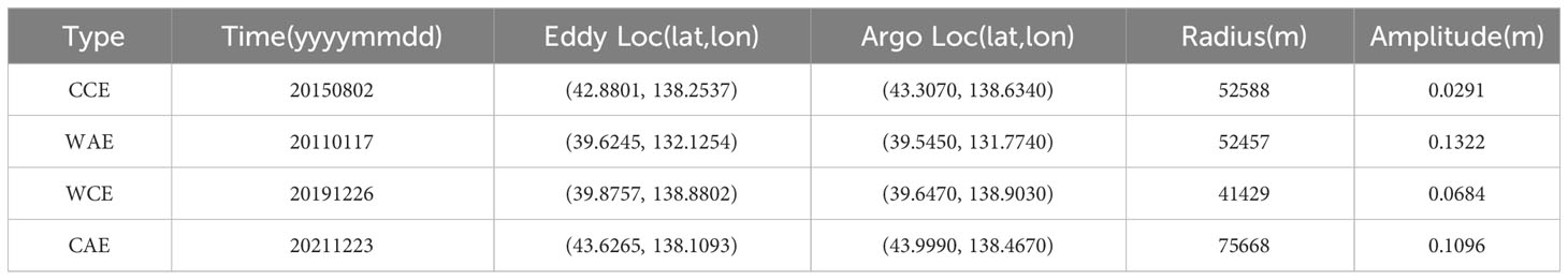
Table 1 Cases of four types of eddies.
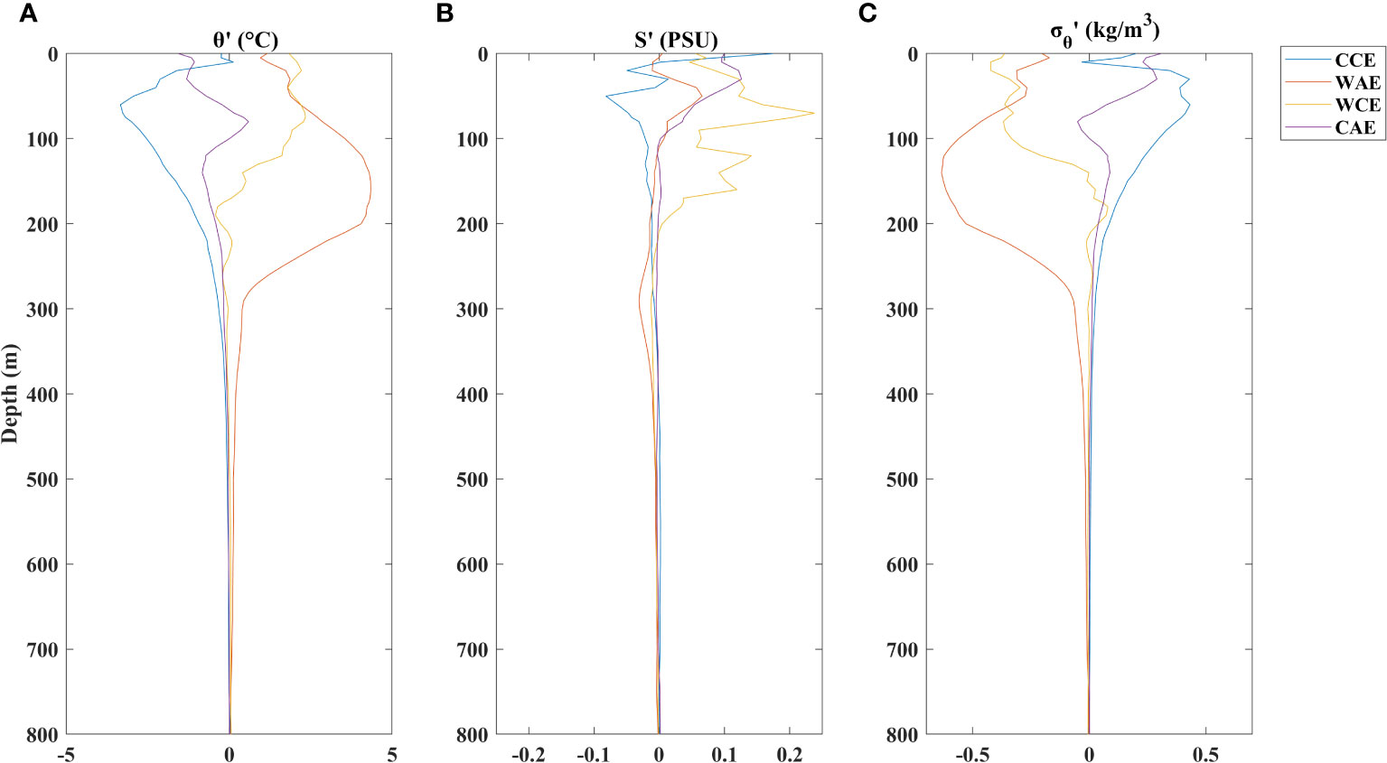
Figure 3 Vertical profiles of (A) temperature anomalies, (B) salinity anomalies (C) potential density anomalies of four types of eddy cases. CCE, Cold cyclonic eddies (blue); WAE, warm anticyclonic eddies (red); WCE, warm cyclonic eddies (yellow), CAE, cold anticyclonic eddies (purple).
3.2 Eddy number variations
There are two ways to define the number of eddies: the Lagrange and Euler methods. The former recognizes the entire life cycle of an eddy as one case, whereas the latter treats eddy snapshots detected at every moment as data points. Here, we adopt the Euler method to statistically analyze normal and abnormal eddies in the Japan/East Sea because it has been revealed in a previous study that some eddies tend to change their temperature sign and then transition between abnormal and normal states during their entire lifespan, especially in the generation and corruption stages (Dilmahamod et al., 2022; Sun et al., 2023). The matching algorithms between eddies and Argo profiles inevitably discard a considerable number of eddy snapshots because only a limited number of eddies capture Argo profiles inside their boundaries. Nevertheless, there is not enough reason to assume that normal and abnormal eddies differ in their capabilities for capturing Argo float profiles. Hence, the results of the statistical analysis can be preliminarily considered to effectively reflect the distribution characteristics of abnormal eddies. Moreover, an Argo float may be caught by an eddy with strong nonlinearity and produce multiple consecutive profiles at a frequency of approximately 5 d. Under these circumstances, profiles with intervals longer than 10 d were selected.
Over the 11-year period from 2011 to 2021, 1358 WAEs, 195 WCEs, 1225 CCEs, and 107 CAEs snapshots were detected in the Japan/East Sea by the aforementioned classification method, accounting for 47.07%, 6.76%, 42.46%, and 3.71% of the total 2885 eddy snapshots, respectively. Figure 4 shows the monthly distribution of the four types of mesoscale eddies. The average number and standard deviation of WAEs, WCEs, CCEs, and CAEs are 113.17 ± 16.00, 16.25 ± 8.17, 102.08 ± 12.77, 8.92 ± 4.68, respectively. The frequency of occurrence of abnormal eddies was substantially lower than that of normal eddies and had higher seasonal fluctuations, according to the standard deviation to mean values ratio. Among the four types of eddies, normal AEs appeared most frequently, whereas abnormal AEs were sparse. The maximum number of each type of eddy occurred in January for WAEs, February for CAEs, December for CCEs, and May for WCEs. Generally, there were more WCEs in the summer and more CAEs in the winter. In addition, it was found that the number of CCEs was less than that of WAEs in most cases but slightly surpassed the latter in July and August. Meanwhile, the number of CAEs was quite low in July and August, when the sea surface temperature of the Japan/East Sea reached its highest value. The monthly distribution of WCEs presents the opposite trend: abnormal cyclonic eddies occur more frequently in spring and summer but rarely appear from September to December.
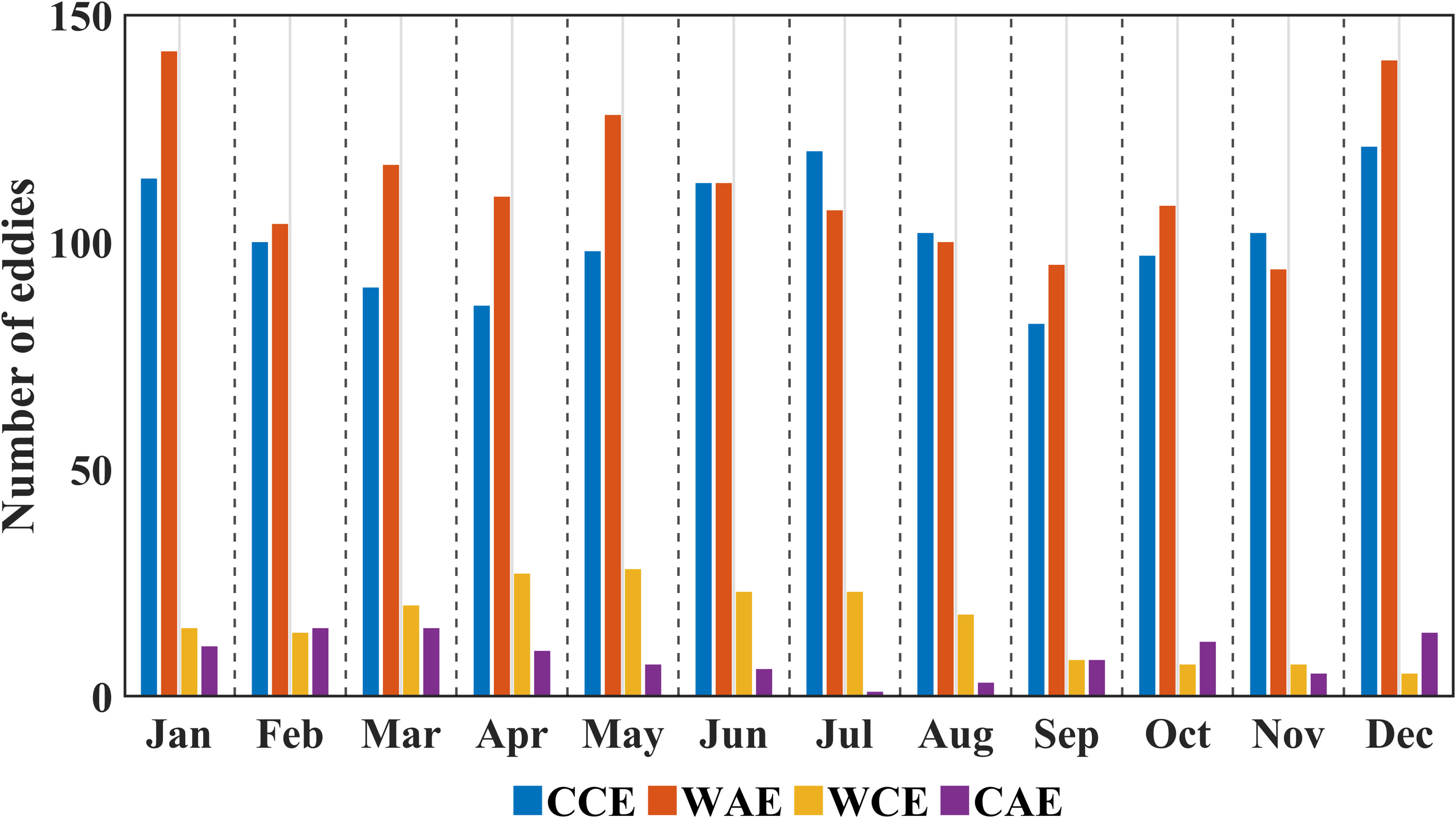
Figure 4 Monthly statistical histogram of 11-year numbers of four categories of eddies during an 11-year period from January 2011 to December 2021. CCE, Cold cyclonic eddies (blue); WAE, warm anticyclonic eddies (red); WCE, warm cyclonic eddies (yellow), CAE, cold anticyclonic eddies (purple).
Figure 5 shows proportions of normal and abnormal eddies in 1° ×1° bins. Normal eddies in the Japan/East Sea, especially in three basins: the Yamato Basin in the southeastern region, the southwestern Tsushima Basin, and the Japan Basin in the north were determined. The cyclonic circulation structure might produce warm anticyclonic eddies along two branches of TWC and a large number of conventional cyclonic eddies in the vicinity of NKCC and LCC, which are the two main cold currents in the western part of the Japan/EastSea. In contrast, two types of abnormal eddies occur sparsely and sporadically in the Japan/East Sea region. The CAEs tend to occur more frequently inside the Tsushima Basin, where EKWC and NKCC encounter each other and generate a subsurface front (Figure 1. Tsugaru Strait, situated between Hokkaido and Honshu, which links the Pacific Ocean and the Japan/East Sea, is also a hotspot for the generation of abnormal eddies. Whereas, WCEs mostly exist in the eastern and northeastern regions of the Japan/East Sea around two warm current branches of Tsushima Warm Current, OB(offshore branch) and NB(nearshore branch).
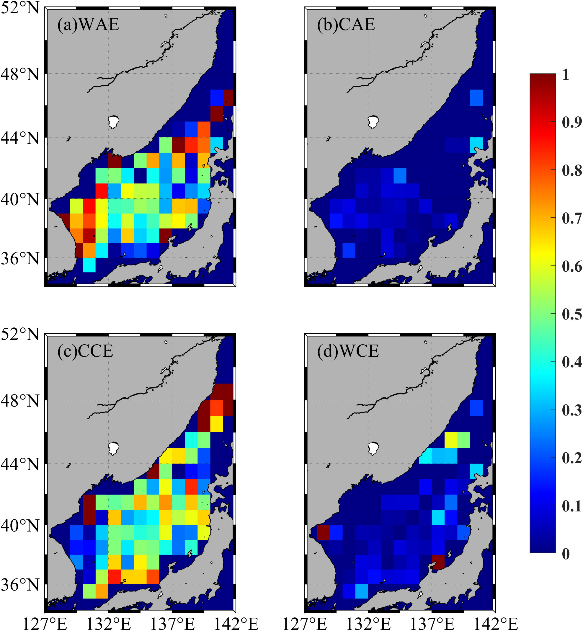
Figure 5 Geographical density heatmaps of the four types of eddies’ in 1° ×1° proportions bins. The number of (A) WAEs, (B) CAEs, (C) CCEs and (D) WCEs is divided by the total number of all types of eddies in the bin from 2011 to 2021.
3.3 Statistical analysis of eddy radius and amplitude
The average number and standard deviation of WAEs, WCEs, CCEs, CAEs radii were 58.50 ± 18.01, 55.05 ± 18.03, 54.17 ± 19.18, and 58.83 ± 22.17 (all counts in km), respectively. Figure 6A compares the radii of CCEs and WCEs. Both present an obvious positive skewness distribution, with a maximum percentage at approximately 45 km. The WCEs’ distribution has a slightly right-deviation peak and a higher occurrence frequency over 60 km especially 90 km than CCEs. In contrast, the CCEs’ appearance percentage was higher than that of WCE but below 50 km as shown in Figure 6B. For normal and abnormal anticyclonic eddies, the distribution peak is located at 65 km and the maximum radius reaches 120 km, which is larger than that of the cyclonic eddies. Unlike WAEs, the radius histogram of the CAEs presented a bimodal distribution with a central low ebb at 60 km and a minor peak at approximately 42 km. The AEs tend to be abnormal when their radius exceeds 100 km, partially because the definition of abnormal anticyclonic eddies permits an individual cold profile, and larger AEs have a stronger capability to absorb cold water masses inside the boundary.
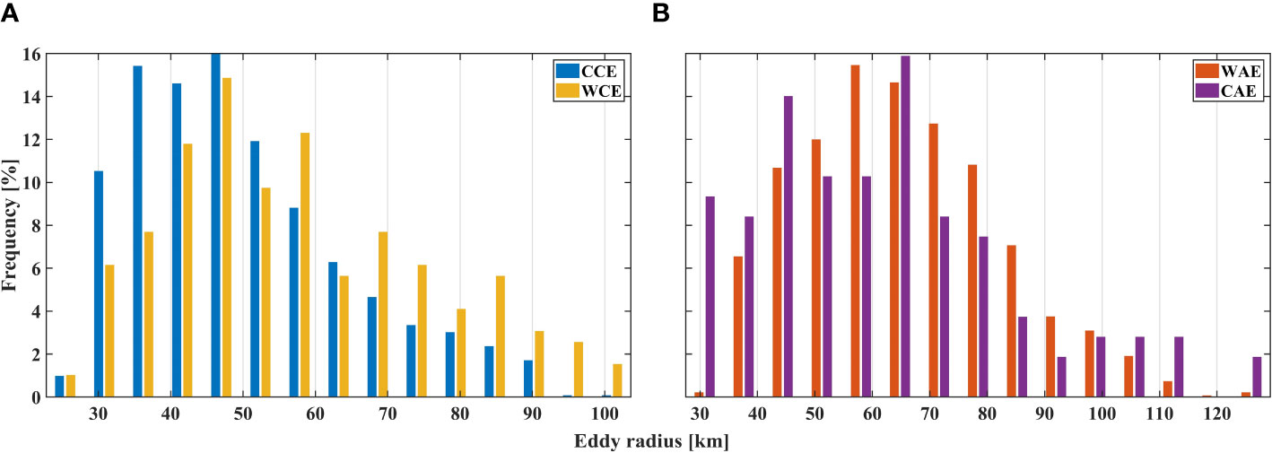
Figure 6 Comparative histogram of the radius of abnormal and normal eddies. (A) comparison between CCEs (blue) and WCEs (yellow) and (B) comparison between WAEs (red) and CAEs (purple).
The statistical distributions of the eddy amplitudes are shown in Figure 7. The average number and standard deviation of WAEs, WCEs, CCEs, and CAEs amplitudes are 8.86 ± 4.57, 6.44 ± 5.48, 5.61 ± 4.22, 9.06 ± 6.14(cm), respectively. Figures 7A, B plot comparative histograms of two cyclonic and anticyclonic eddies, respectively. Cyclonic eddies have a more concentrated distribution than anticyclonic eddies, and the frequency peaks of the eddy amplitudes of CCEs and WCEs located at approximately 3 cm and reach 25 and 30%, respectively. In comparison, the distribution of WAEs and CAEs is even greater, with no frequency exceeding 15%. The distribution peak of WAEs occurred at approximately 12 cm and CAEs mostly appeared at a radius of approximately 3 cm.
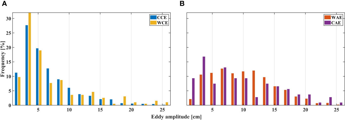
Figure 7 As in Figure 6, but for eddy amplitude. (A) comparison between CCEs (blue) and WCEs (yellow) and (B) comparison between WAEs (red) and CAEs (purple).
3.4 Composite vertical structures of abnormal and normal eddies
Figures 8–10 present the vertical section of composite eddies’ temperature, salinity and potential density anomalies along Δy = 0 of abnormal and normal eddies for comparison. The conventional composite AE/CE is associated with a positive/negative temperature anomaly core (Figures 8A, C). The warm core of the composite WAE had a maximum temperature anomaly of approximately +2.1° centered at ∼ 180 m. In comparison, the cold core of the composite CCE was confined to approximately 120 m with a magnitude of approximately -1.7°. Below the core, the intensities of both composite normal eddies damped rapidly to less than ±0.2° below 300 m. Regarding abnormal eddies, the composite WCE had a lower temperature anomaly intensity than the traditional warm anticyclonic eddies. Its core was located in the upper 100 m and had a maximum temperature anomaly of approximately +1.0°. Meanwhile, the intensity of the composite CAE’s core was slightly higher than that of the composite WCE but still weaker than that of the conventional cyclonic eddy. The minimum temperature anomaly was approximately -1.1° at ∼ 50 m. The impact of the two composite abnormal eddies on the temperature variation was limited to a depth of 200 m.
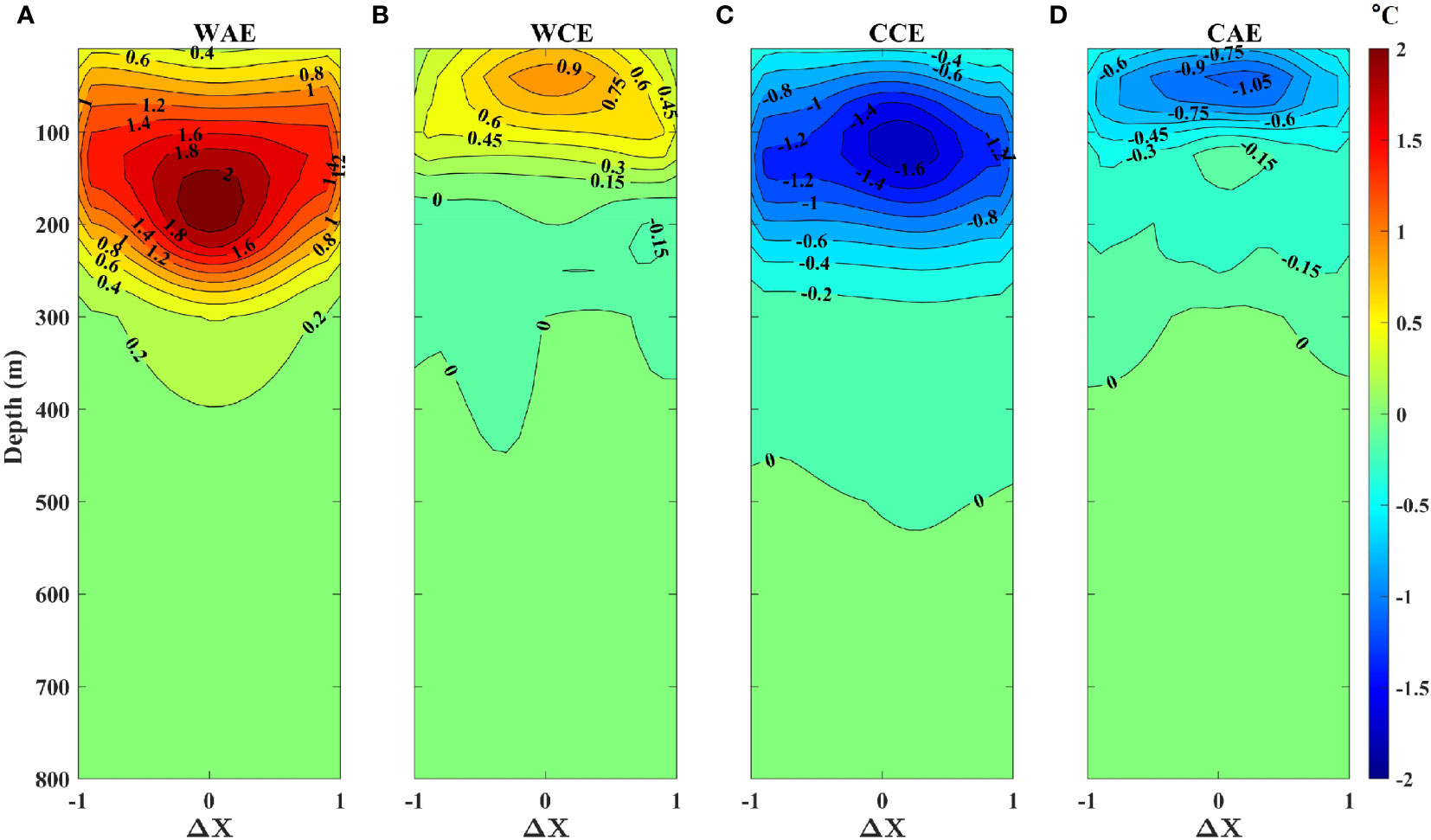
Figure 8 Zonal temperature anomaly sections along Δy = 0 across the four types of composite mesoscale eddies. Vertical structures of the temperature anomalies (°C) of composite (A) WAE, (B) WCE, (C) CCE, and (D) CAE are present in the form of contour maps.
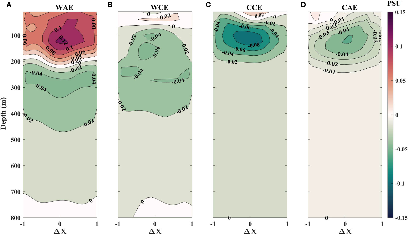
Figure 9 As in Figure 8, but for salinity anomalies. Vertical structures of the salinityanomalies (PSU) of composite (A) WAE, (B) WCE, (C) CCE, and (D) CAE are present in the form of contour maps.
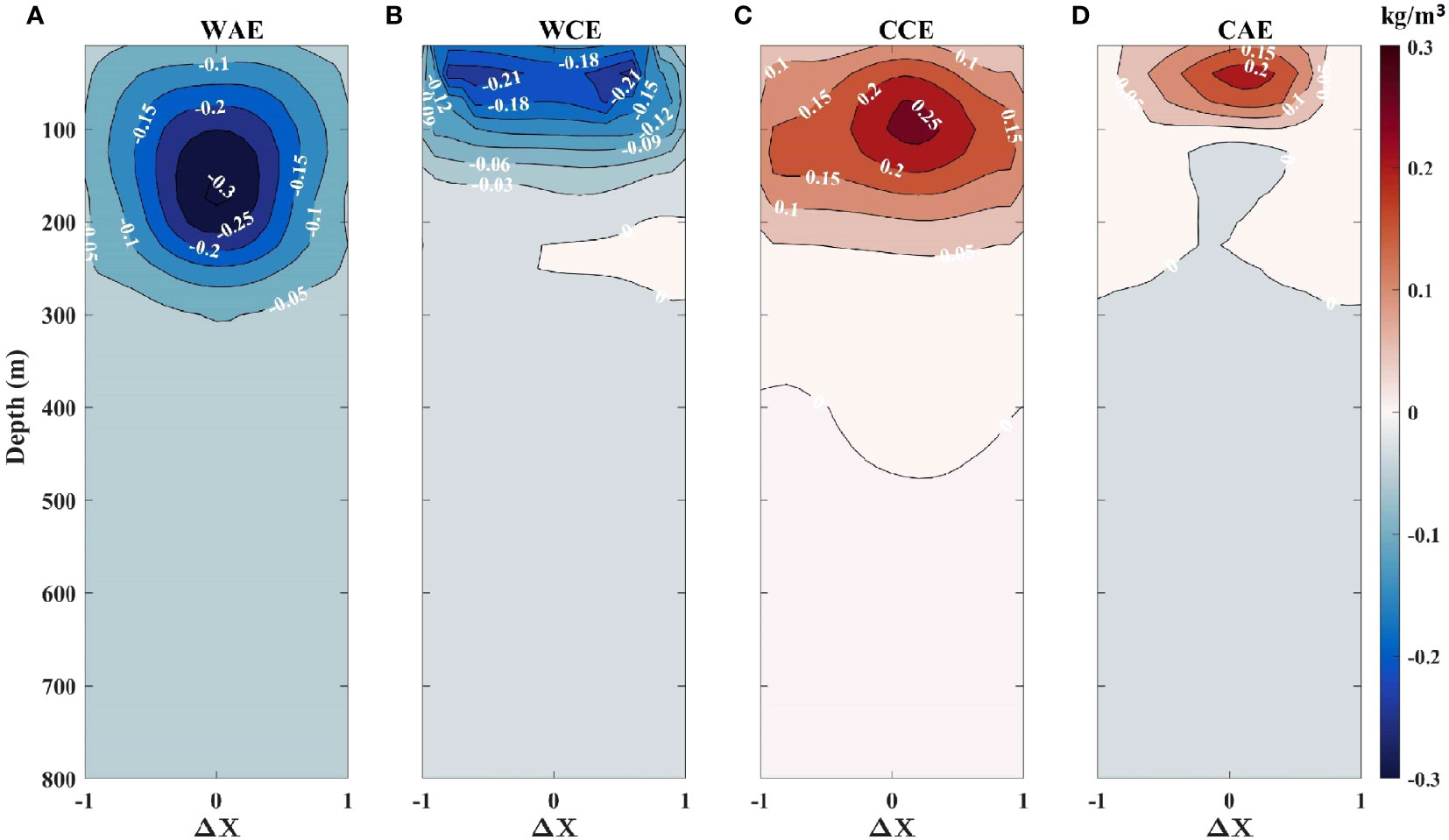
Figure 10 As in Figure 8, but for potential density anomalies. Vertical structures of the potential density anomalies (kg/m³) of composite (A) WAE, (B) WCE, (C) CCE, and (D) CAE are present in the form of contour maps.
The vertical structures of the composite salinity anomalies are shown in Figure 9. The salinity anomaly of the composite WAE presents a typical double-core structure: one upper saltier core with a maximum intensity of ∼+0.12 psu at 200 m and another lower fresh core with a negative salinity anomaly of approximately ∼-0.04 psu below 200 m was found in a previous study (Itoh and Yasuda, 2010). In contrast, composite CCE has a single-core vertical structure of negative salinity anomaly, in which the minimum intensity reaches -0.08 psu. The composite WCE had the same double-core structure as the composite WAE. In the upper 50 m, the salinity anomaly was positive and the sign of the anomaly reversed as depth increased. The minimum value of salinity anomaly of composite WCE was approximately -0.04 psu. The vertical salinity structure of the composite CAE was similar to that of CCE but had a weaker core of approximately -0.05 psu.
The distribution of the potential density anomalies of the four types of eddies resembled the structure of the temperature anomalies. The composite WAE and WCE both had a light core with a minimum anomaly value of -0.3(-0.21)kg/m3 at ∼180(50)m. Comparatively, the dense cores of the composite CCE and CAE reached a maximum magnitude(+0.25 kg/m3 for CCE and +0.2 for CAE) of the potential density anomaly at approximately 100 m and 50 m, respectively. The influence of depth of the composite WAE was the greatest, reaching ∼300 m. Both composite abnormal eddies and WCEs/CAEs could only affect the potential density of the water mass in the upper 150 m/100 m.
To better present the three-dimensional physical field structure of the two types of composite abnormal eddies, horizontal slices of the temperature, salinity, and potential density anomalies at several selected depths (10,25,50,75,100 m) within the composite WCE/CAE are shown in Figures 11, 12. Geostrophic current anomalies of the composite abnormal eddies were calculated by using the following thermal wind relationship in Equations 3, 4 (Vallis, 2006):
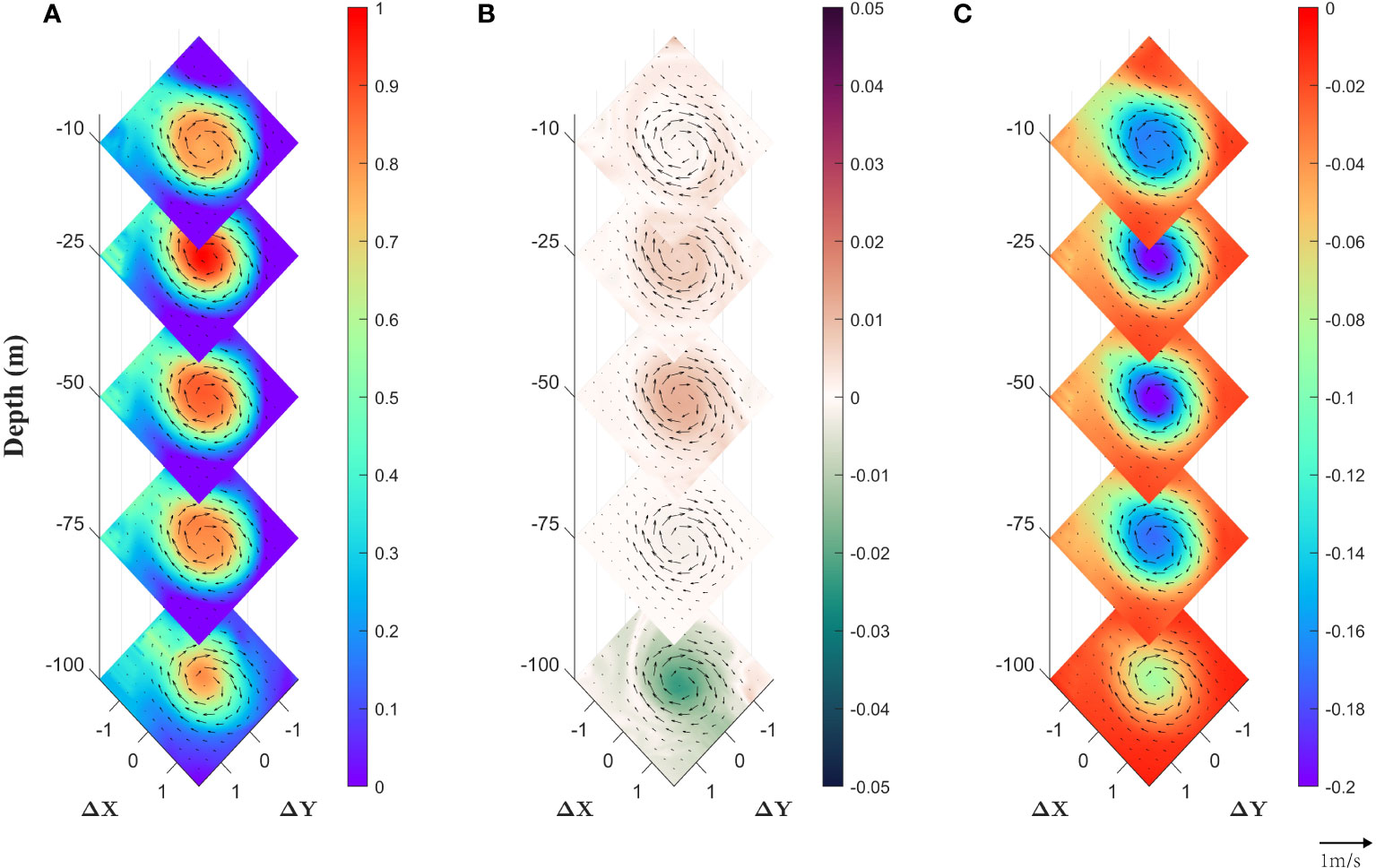
Figure 11 Three-dimensional structure of composite WCE. Anomalies of (A) temperature (°C) (B) salinity (PSU) (C) potential density (kg/m3) overlayed with geostrophic current speed anomaly (cm/s) at 10, 25, 50, 75, 100m are shown as three five-layer sliced diagrams.
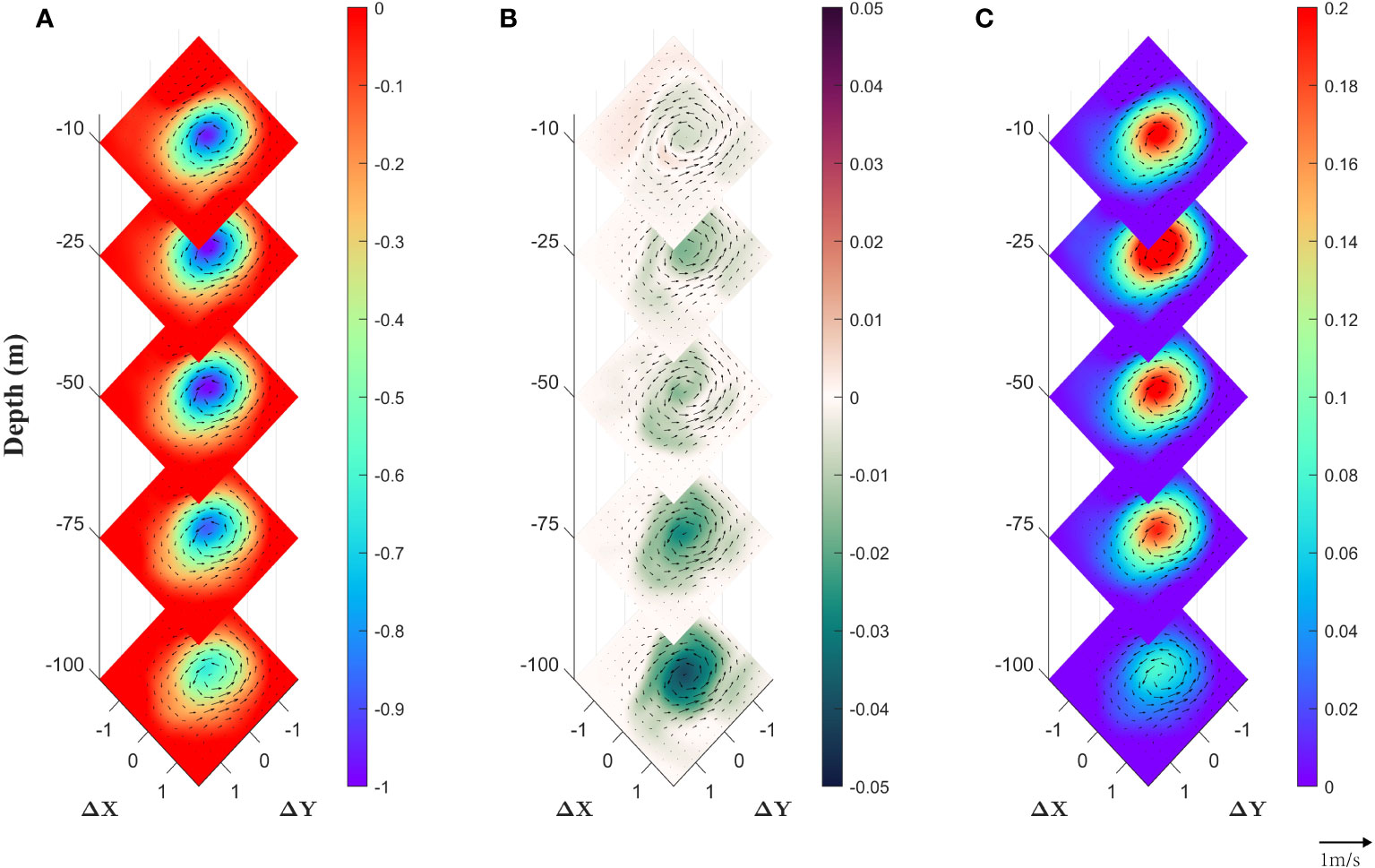
Figure 12 As in Figure 11, but for composite CAE. Anomalies of (A) temperature (°C) (B) salinity (PSU) (C) potential density (kg/m3) overlayed with geostrophic current speed anomaly (cm/s) at 10, 25, 50, 75, 100m are shown as three five-layer sliced diagrams.
where u(v) is the zonal (meridional) component of the geostrophic current velocity, f is the local Coriolis parameter (here, the average latitude of the eddies is composited to calculate f and ρ0 = 1.024g/cm3 is the reference density of seawater). The formula is the quantification of geostrophic equilibrium and provides the subsurface distribution of velocity anomalies after integration.
This is shown in Figures 11, 12 that the three-dimensional structure of composite WCE and CAE is identical to the aforementioned vertical structure revealed by the section diagram. The maximum magnitude of the temperature and potential density anomalies occurs between 25 m and 50 m and the eddy influence was confined to the upper 100 m for both abnormal eddies. The vertical distribution of geostrophic velocity anomaly was similar to that of the above tracers. At approximately 25 m, both composite abnormal eddies reached maximum subsurface speeds of approximately 0.3m/s. The geostrophic velocity of the abnormal eddies decreases rapidly below 100 m. In addition, the cyclonic/anticyclonic circulation structure for the flow field of the composite WCE/CAE showed that the rotation direction of abnormal eddies was consistent with that of normal eddies and was closely associated with sea-surface height anomalies.
4 Discussion
4.1 Meridional heat and salt transport of abnormal eddies
Mesoscale eddies deeply involve in ocean heat and salt transport(Qiu and Chen, 2005; Chaigneau et al., 2011; Yang et al., 2015). Since the existence of abnormal eddies was long neglected, it is necessary to evaluate their impacts on ocean heat/salt transport. With the composite structure of temperature, salt and geostrophic current anomalies of abnormal eddies in the Japan/East Sea, meridional heat and salt fluxes induced by WCE and CAE were then estimated as follow (Yang et al., 2015), where ρ0 and Cp are the reference density and heat capacity at constant pressure, respectively in Equations 5 and 6:
It is shown in Figures 13A, B that the meridional heat fluxes of two types of abnormal eddies share an approximate symmetrical structure with positive heat transport in the east part and negative transport in the west part. The heat fluxes of composite WCE/CAE are mainly confined in the upper 200m. The maximum heat flux value of composite CAE is located at about 25m while composite WCE shows strongest transport capacity at ∼ 75m. As for composite WCE, positive heat fluxes in the east part(with a maximum magnitude over 1.2×10⁶Wm−2) are obviously stronger than negative heat fluxes in the west part. Negative heat fluxes appear in the top right part of the vertical section of composite CAE’s heat transport. An approximate symmetrical structure of heat fluxes occurs between 50m and 100m of the composite CAE. The total integration of meridional heat transport of composite WCE(CAE) is 1.17 × 10⁷(−3.44 × 10⁵)Wm−2, indicating a north(south but weak) heat transport in the Japan/East Sea.
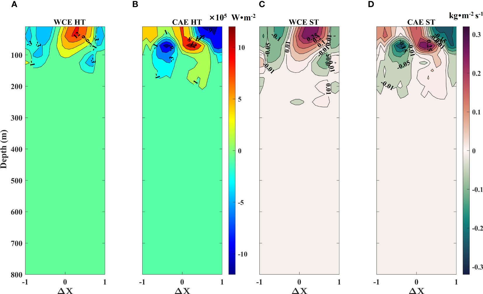
Figure 13 Vertical sections of meridional heat and salt transport of two types of composite abnormal eddies (WCE, CAE) along Δy = 0. (A) heat transport of composite WCE, (B) heat transport of composite CAE, (C) salt transport of composite WCE, (D) salt transport of composite WCE. HT, heat transport; ST, salt transport.
Vertical structures of meridional salt transport of two abnormal eddies are similar with that of heat transport. As shown in Figures 13C, D, composite WCE has a north salt transport with a maximum magnitude of 0.25kgm−2s−1 in the east part and south salt transport with an amplitude of about −0.1kgm−2s−1. Integration of salt transport of composite WCE(CAE) is 2.80(-0.08)kgm−2s−1, showing the same results compared with meridional heat transport: WCE in this region transport heat and salt northerly and CAE has weaker transport capacity.
4.2 Generation mechanisms of abnormal eddies
Three possible mechanisms were proposed to explain the generation and occurrence of these abnormal eddies. The first is the influence of the surrounding background field of the eddies. Itoh and Yasuda (2010) found that 15% of the anticyclonic eddies in the western boundary region of the subarctic north pacific had a cold and fresh core. Two main mechanisms were proposed: (1) Conventional AEs that originated from Kuroshio Extension were converted to having cold cores after encountering Oyashio water. (2) Extremely cold, fresh, and low-potential-vorticity water derived from the Sea of Okhotsk formed cold anticyclonic eddies. Similarly, the encounter of warm and cold currents (OB and LCC in the northern Japan Basin, and NKCC and EKWC on the east coast of Korean Peninsula) might explain the high incidence of abnormal cyclonic eddies at these places. In addition, it can be inferred that anticyclonic warm eddies shed from southern warm currents are induced to transition into cold eddies after encountering the northern cold current, which may be the main generation mechanism of CAEs. The second-generation mechanism of abnormal eddies is wind-stress-induced Ekman pumping (Ni et al., 2023) with a shallow surface mixed layer and surface heating/cooling. It can be seen that CAEs occurred more frequently in Dec, Jan, Feb and Mar, when the strong cold northeast monsoon prevails in the Japan/East Sea. Meanwhile, there were more WCEs in spring and summer when the surface winds over the Japan/East Sea were weak and varied with increasing temperature. However, the relationship between wind-stress-induced Ekman pumping and the generation mechanism of abnormal eddies in the Japan/East Sea region requires further research. The last mechanism is subsurface-intensified baroclinic instability, which has been found to be closely connected to subsurface mesoscale eddies (Feng et al., 2021), which can generate opposite temperature signals in the upper ocean and are recognized as abnormal eddies (Qi et al., 2022). In addition, the growth and decay stages of eddies with baroclinic energy conversion are high-incidence periods for abnormal eddies (Sun et al., 2019).
5 Conclusion
Based on a synergistic investigation of satellite altimetry and Argo profile data during the period of 2011-2021, the spatiotemporal characteristics and composite 3D structure of abnormal eddies in the Japan/East Sea were first obtained via classification criteria based on the heat content anomaly and eddy composite method. The distribution and characteristics of the normal eddies were also investigated for comparison. A total of 1358 WAEs, 195 WCEs, 1225 CCEs, and 107 CAEs were detected in the Japan/East Sea from 2011 to 2021, accounting for 47.07%, 6.76%, 42.46%, and 3.71% of the 2885 eddies. Approximately 10% of mesoscale eddies in the Japan/East Sea present distinctly abnormal features, while the remaining 10% are conventional. Comparing to previous detection results of abnormal eddies in global ocean (Ni et al., 2021), the proportion of WCEs and CAEs in the Japan/East Sea is slightly less than that in the tropical oceans but exceeds that in the rest part of the ocean.
The monthly distribution of the number of abnormal eddies shows stronger fluctuation; WCEs tend to occur more frequently in the summer, and CAEs were more common in winter and early spring, resembling normal eddies(CCEs and WAEs), but with less fluctuation. The spatial distribution of the four types of eddies is presented through geographical heatmaps in 1° ×1°, and the locations of the abnormal and normal eddy snapshots are relevant to the cyclonic circulation structure in the Japan/East Sea to a certain content.
Statistical analysis of the radii and amplitude-s of the four eddy categories was conducted by presenting comparative histograms of the radii and amplitudes of the abnormal and corresponding normal eddies. The histograms of the radii and amplitudes of WCEs, CCEs and WAEs show an obvious positive skewness distribution, consistent with previous studies(Chelton et al., 2011b), whereas the distribution of CAEs’ radii and amplitudes of the CAEs is multimodal. The average radii of the four types of eddies were nearly the same (∼ 56km), whereas the average amplitudes of the two types of anticyclonic eddies (∼ 9cm) were larger than those of the two cyclonic eddies (∼ 6cm).
Based on the results of the synergy investigation, three-dimensional structures of the temperature, salinity, and potential density anomalies of abnormal eddies were acquired using the composite method (vertical sections of composite normal eddies were also plotted for comparison). The warm and light core of the composite WCE is located at approximately 50 m. The surface positive salinity anomaly and negative anomaly were below 100 m of WCE. The composite CAE has a cold and dense core at the same depth, sharing a similar salinity distribution. The geostrophic velocity anomalies of abnormal eddies were found to have directions identical to those of normal eddies, that is, the flow field of CAE(WCE) was anticyclonic(cyclonic).
Research on eddies with abnormal cores in the Japan/East Sea is of great importance for re-evaluating the environmental effects caused by mesoscale eddies, such as heat/salt transport, changes in mixed layer depth, air-sea interaction, hydroacoustic transmission, and other physical processes in the Japan/East Sea and other regions. Moreover, the physical mechanisms of generation and maintenance of abnormal eddies require further clarification and investigation based on multi-source data such as numerical models and in-situ data in follow-up studies.
Data availability statement
The original contributions presented in the study are included in the article/supplementary material. Further inquiries can be directed to the corresponding author.
Author contributions
YM: Conceptualization, Data curation, Investigation, Methodology, Visualization, Writing – original draft. QL: Conceptualization, Supervision, Writing – original draft. HW: Conceptualization, Supervision, Writing – original draft. XY: Conceptualization, Supervision, Writing – original draft. SL: Supervision, Writing – original draft.
Funding
The author(s) declare that no financial support was received for the research, authorship, and/or publication of this article.
Acknowledgments
Daily SLA data and mesoscale eddy trajectory atlas products from AVISO(https://www.aviso.altimetry.fr) were used. Argo profiles were collected from https://data-argo.ifremer.fr/ and CARS2009 climatological atlas was downloaded from CSIRO(https://www.marine.csiro.au/dunn/cars2009/).
Conflict of interest
The authors declare that the research was conducted in the absence of any commercial or financial relationships that could be construed as a potential conflict of interest.
Publisher’s note
All claims expressed in this article are solely those of the authors and do not necessarily represent those of their affiliated organizations, or those of the publisher, the editors and the reviewers. Any product that may be evaluated in this article, or claim that may be made by its manufacturer, is not guaranteed or endorsed by the publisher.
References
Akima H. (1970). A new method of interpolation and smooth curve fitting based on local procedures. J. ACM 17, 589–602. doi: 10.1145/321607.321609
Amores A., Melnichenko O., Maximenko N. (2016). Coherent mesoscale eddies in the North Atlantic subtropical gyre: 3D structure and transport with application to the salinity maximum. J. Geophys. Res.: Oceans 122. doi: 10.1002/2016JC012256
An M., Liu J., Liu J., Sun W., Yang J., Tan W., et al. (2022). Comparative analysis of four types of mesoscale eddies in the north pacific subtropical countercurrent region – part I spatial characteristics. Front. Mar. Sci. 9. doi: 10.3389/fmars.2022.1004300
Barth A., Beckers J.-M., Troupin C., Alvera-Azcárate A., Vandenbulcke L. (2014). divand-1.0: n-dimensional variational data analysis for ocean observations. Geosci. Model. Dev. 7, 225–241. doi: 10.5194/gmd-7-225-2014
Chaigneau A., Le Texier M., Eldin G., Grados C., Pizarro O. (2011). Vertical structure of mesoscale eddies in the eastern South Pacific Ocean: A composite analysis from altimetry and Argo profiling floats. J. Geophys. Res.: Oceans 116. doi: 10.1029/2011JC007134
Chelton D. B., Gaube P., Schlax M. G., Early J. J., Samelson R. M. (2011a). The influence of nonlinear mesoscale eddies on near-surface oceanic chlorophyll. Science 334, 328–332. doi: 10.1126/science.1208897
Chelton D. B., Schlax M. G., Samelson R. M. (2011b). Global observations of nonlinear mesoscale eddies. Prog. Oceanogr. 91, 167–216. doi: 10.1016/j.pocean.2011.01.002
Dilmahamod A. F., Karstensen J., Dietze H., Löptien U., Fennel K. (2022). Generation mechanisms of mesoscale eddies in the Mauritanian upwelling region. J. Phys. Oceanogr. 52, 161–182. doi: 10.1175/JPO-D-21-0092.1
Dong C., McWilliams J. C., Liu Y., Chen D. (2014). Global heat and salt transports by eddy movement. Nat. Commun. 5, 3294. doi: 10.1038/ncomms4294
Ducet N., Le Traon P. Y., Reverdin G. (2000). Global high-resolution mapping of ocean circulation from topex/poseidon and ers-1 and -2. J. Geophys. Res.: Oceans 105, 19477–19498. doi: 10.1029/2000JC900063
Faghmous J. H., Frenger I., Yao Y., Warmka R., Lindell A., Kumar V. (2015). A daily global mesoscale ocean eddy dataset from satellite altimetry. Sci. Data 2, 150028. doi: 10.1038/sdata.2015.28
Feng L., Liu C., Köhl A., Stammer D., Wang F. (2021). Four types of baroclinic instability waves in the global oceans and the implications for the vertical structure of mesoscale eddies. J. Geophys. Res.: Oceans 126, e2020JC016966. doi: 10.1029/2020JC016966
Frenger I., Gruber N., Knutti R., Münnich M. (2013). Imprint of Southern Ocean eddies on winds, clouds and rainfall. Nat. Geosci. 6, 608–612. doi: 10.1038/ngeo1863
He Y., Feng M., Xie J., He Q., Liu J., Xu J., et al. (2021). Revisit the vertical structure of the eddies and eddy-induced transport in the leeuwin current system. J. Geophys. Res.: Oceans 126, e2020JC016556. doi: 10.1029/2020JC016556
Hosoda K., Hanawa K. (2004). Anticyclonic eddy revealing low sea surface temperature in the sea South of Japan: case study of the eddy observed in 1999–2000. J. Oceanogr. 60, 663–671. doi: 10.1007/s10872-004-5759-9
Itoh S., Kaneko H., Kouketsu S., Okunishi T., Tsutsumi E., Ogawa H., et al. (2021). Vertical eddy diffusivity in the subsurface pycnocline across the Pacific. J. Oceanogr. 77, 185–197. doi: 10.1007/s10872-020-00589-9
Itoh S., Yasuda I. (2010). Water mass structure of warm and cold anticyclonic eddies in the western boundary region of the subarctic North Pacific. J. Phys. Oceanogr. 40, 2624–2642. doi: 10.1175/2010JPO4475.1
Jacobs G. A., Hogan P. J., Whitmer K. R. (1999). Effects of eddy variability on the circulation of the Japan/east sea. J. Oceanogr. 55, 247–256. doi: 10.1023/A:1007898131004
Kahru M., Mitchell B. G., Gille S. T., Hewes C. D., Holm-Hansen O. (2007). Eddies enhance biological production in the weddell-scotia confluence of the southern ocean. Geophys. Res. Lett. 34. doi: 10.1029/2007GL030430
Lee D.-K., Niiler P. (2010). Eddies in the Southwestern East/Japan sea. Deep Sea Res. Part I: Oceanogr. Res. Pap. 57, 1233–1242. doi: 10.1016/j.dsr.2010.06.002
Liu S., Xu J., Qiao L., Li G., Shi J., Ding D., et al. (2023). Spatial-temporal variations of short-lived mesoscale eddies and their environmental effects. Front. Mar. Sci. 10. doi: 10.3389/fmars.2023.1069897
Liu Y., Zheng Q., Li X. (2021). Characteristics of global ocean abnormal mesoscale eddies derived from the fusion of sea surface height and temperature data by deep learning. Geophys. Res. Lett. 48, e2021GL094772. doi: 10.1029/2021GL094772
Morimoto A., Yanagi T., Kaneko A. (2000). Eddy field in the Japan sea derived from satellite altimetric data. J. Oceanogr. 56, 449–462. doi: 10.1023/A:1011184523983
Nagai T., Gruber N., Frenzel H., Lachkar Z., McWilliams J. C., Plattner G.-K. (2015). Dominant role of eddies and filaments in the offshore transport of carbon and nutrients in the california current system. J. Geophys. Res.: Oceans 120, 5318–5341. doi: 10.1002/2015JC010889
Ni Q., Zhai X., Jiang X., Chen D. (2021). Abundant cold anticyclonic eddies and warm cyclonic eddies in the global ocean. J. Phys. Oceanogr. 51, 2793–2806. doi: 10.1175/JPO-D-21-0010.1
Ni Q., Zhai X., Yang Z., Chen D. (2023). Generation of cold anticyclonic eddies and warm cyclonic eddies in the tropical oceans. J. Phys. Oceanogr. 53, 1485–1498. doi: 10.1175/JPO-D-22-0197.1
Pascual A., Faugère Y., Larnicol G., Le Traon P.-Y. (2006). Improved description of the ocean mesoscale variability by combining four satellite altimeters. Geophys. Res. Lett. 33. doi: 10.1029/2005GL024633
Pegliasco C., Delepoulle A., Mason E., Morrow R., Faugère Y., Dibarboure G. (2022). META3.1exp: a new global mesoscale eddy trajectory atlas derived from altimetry. Earth System Sci. Data 14, 1087–1107. doi: 10.5194/essd-14-1087-2022
Qi Y., Mao H., Du Y., Li X., Yang Z., Xu K., et al. (2022). A lens-shaped, cold-core anticyclonic surface eddy in the northern South China Sea. Front. Mar. Sci. 9. doi: 10.3389/fmars.2022.976273
Qiu B., Chen S. (2005). Eddy-induced heat transport in the subtropical north pacific from argo, tmi, and altimetry measurements. J. Phys. Oceanogr. 35, 458–473. doi: 10.1175/JPO2696.1
Seo H., O’Neill L. W., Bourassa M. A., Czaja A., Drushka K., Edson J. B., et al. (2023). Ocean mesoscale and frontal-scale ocean–atmosphere interactions and influence on large-scale climate: A review. J. Climate 36, 1981–2013. doi: 10.1175/JCLI-D-21-0982.1
Siegel D. A., Peterson P., McGillicuddy D. J. Jr., Maritorena S., Nelson N. B. (2011). Biooptical footprints created by mesoscale eddies in the sargasso sea. Geophys. Res. Lett. 38. doi: 10.1029/2011GL047660
Sun W., An M., Liu J., Liu J., Yang J., Tan W., et al. (2023). Comparative analysis of four types of mesoscale eddies in the North Pacific Subtropical Countercurrent region - part II seasonal variation. Front. Mar. Sci. 10. doi: 10.3389/fmars.2023.1121731
Sun W., Dong C., Tan W., He Y. (2019). Statistical characteristics of cyclonic warm-core eddies and anticyclonic cold-core eddies in the North Pacific based on remote sensing data. Remote Sens. 11, 208. doi: 10.3390/rs11020208
Vallis G. K. (2006). Atmospheric and Oceanic Fluid Dynamics (Cambridge, U.K: Cambridge University Press).
Wang Y., Zhang H.-R., Chai F., Yuan Y. (2018). Impact of mesoscale eddies on chlorophyll variability off the coast of Chile. PloS One 13, e0203598. doi: 10.1371/journal.pone.0203598
Yan X., Kang D., Pang C., Zhang L., Liu H. (2022). Energetics analysis of the eddy–kuroshio interaction east of Taiwan. J. Phys. Oceanogr. 52, 647–664. doi: 10.1175/JPO-D-21-0198.1
Yang G., Wang F., Li Y., Lin P. (2013). Mesoscale eddies in the northwestern subtropical Pacific Ocean: Statistical characteristics and three-dimensional structures. J. Geophys. Res.: Oceans 118, 1906–1925. doi: 10.1002/jgrc.20164
Yang G., Yu W., Yuan Y., Zhao X., Wang F., Chen G., et al. (2015). Characteristics, vertical structures, and heat/salt transports of mesoscale eddies in the southeastern tropical Indian Ocean. J. Geophys. Res.: Oceans 120, 6733–6750. doi: 10.1002/2015JC011130
Zhang W.-Z., Ni Q., Xue H. (2018). Composite eddy structures on both sides of the Luzon Strait and influence factors. Ocean Dynam. 68, 1527–1541. doi: 10.1007/s10236-018-1207-z
Zhang Z., Wang Y., Qiu B. (2014). Oceanic mass transport by mesoscale eddies. Sci. (New York N.Y.) 345, 322–324. doi: 10.1126/science.1252418
Keywords: abnormal eddy, Japan/East Sea, composite analysis, mesoscale eddy, spatiotemporal characteristics, vertical structures
Citation: Ma Y, Li Q, Wang H, Yu X and Li S (2024) Composite vertical structures and spatiotemporal characteristics of abnormal eddies in the Japan/East Sea: a synergistic investigation using satellite altimetry and Argo profiles. Front. Mar. Sci. 10:1309513. doi: 10.3389/fmars.2023.1309513
Received: 08 October 2023; Accepted: 26 December 2023;
Published: 24 January 2024.
Edited by:
Francisco Machín, University of Las Palmas de Gran Canaria, SpainReviewed by:
Jihai Dong, Nanjing University of Information Science and Technology, ChinaYuntao Wang, Ministry of Natural Resources, China
Huabing Xu, Guangdong Ocean University, China
Copyright © 2024 Ma, Li, Wang, Yu and Li. This is an open-access article distributed under the terms of the Creative Commons Attribution License (CC BY). The use, distribution or reproduction in other forums is permitted, provided the original author(s) and the copyright owner(s) are credited and that the original publication in this journal is cited, in accordance with accepted academic practice. No use, distribution or reproduction is permitted which does not comply with these terms.
*Correspondence: Qinghong Li, bGlxaDc4QDE2My5jb20=