 Jasen R. Jacobsen
 Christopher A. Edwards
 Brian S. Powell
 John A. Colosi1
 Jerome Fiechter
94% of researchers rate our articles as excellent or good
Learn more about the work of our research integrity team to safeguard the quality of each article we publish.
Find out more
ORIGINAL RESEARCH article
Front. Mar. Sci., 14 December 2023
Sec. Marine Biogeochemistry
Volume 10 - 2023 | https://doi.org/10.3389/fmars.2023.1309011
This article is part of the Research TopicBiogeochemical Responses to Physical Processes in the North Pacific and Its Adjacent Marginal SeasView all 9 articles
When the barotropic tide encounters variable bathymetry, fluctuating flow along a topographic slope generates baroclinic tides, or internal tides. There is growing evidence that these internal tides can affect primary production in the euphotic zone, though the dominant mechanisms are unclear. Internal tides move passive phytoplankton through an exponentially varying light field, enhancing primary production near the base of the euphotic zone. In addition internal tides also increase primary production through vertical nutrient advection into the euphotic zone. Topographically generated internal tides can be separated into two regimes: 1) the often highly nonlinear near-field regime where tidal beams are observed and 2) the more linear far-field regime. This study examines the primary production response to these internal tide processes using the Regional Ocean Modeling System (ROMS) coupled to a simple Nutrient, Phytoplankton, Zooplankton, Detritus (NPZD) model configured for an oligotrophic system with the nutricline positioned below 50 m depth. These idealized simulations generate internal tide beams with an oscillating, horizontal body force at the M2 tidal frequency that is applied to domains with a bathymetric step and uniform stratification. Sensitivity of the primary production response to the energy content of the tidal beam is obtained by adjusting the height and slope of the bathymetric step. Simulation results reveal that primary production intensifies along tidal beams due to the local enhancement of parcel vertical displacement (light effect) and nutrient advective flux divergence (nutrient effect). In the near-field regime across the range of step heights and slopes in this study, the nutrient effect is an order of magnitude larger and explains 92% of the variance in primary production versus only 14% for the light effect. The geometry of the generating feature sets the kinematics of the tidal beam. The light effect is limited in the euphotic zone across our domains because realized changes in light experienced over a tidal cycle are small relative to the amount of light available at a particular depth. In contrast, the magnitude of the nutrient effect increases more substantially with tidal beam energy.
Internal waves are ubiquitous throughout the global ocean and, near their generation sites, affect primary production by two mechanisms. As internal waves propagate, they displace passive phytoplankton vertically through the water column, increasing the irradiance available for primary production (Lande and Yentsch (1988); Holloway and Denman (1989); Evans et al. (2008); Garwood et al. (2020)). Internal waves may also affect primary production by enhancing the vertical supply of nutrients to the euphotic zone (Althaus et al. (2003); Holligan et al. (1985); Granata et al. (1995); Sharples et al. (2009); Sharples et al. (2007); Lucas et al. (2011); Stevens et al. (2012); Villamaña et al. (2017); Tuerena et al. (2019)). However, the relative contributions of the light and nutrient effects of internal waves on primary production are not clearly defined. By diagnosing the governing mechanism through which internal waves affect primary production, we gain insight into how the baseline primary production is controlled in areas above sloping bathymetry.
Some of the largest internal waves in the world are associated with internal tide generation at bathymetric features by barotropic tides (e. g. Luzon Straight: Kerry et al. (2013); Pichon et al. (2013), Hawaii: Rudnick (2003); Cole et al. (2009), and Tasmania: Waterhouse et al. (2018)). By a variety of mechanisms internal tides can be formed (critical slopes, lee waves, etc.) and in many cases the initial character of the wave is a beam with directed energy propagation (group velocity) at an angle (θCɡ) determined by the stratification (), the frequency of the wave (ω), and the inertial frequency (f). The ray theory relation is given by Cushman-Roisin and Beckers (2011) as
In addition, the beam can also be interpreted as a superposition of many normal modes at the frequency ω with different eigenwavenumbers (Colosi (2016)). Observations indicate that the beam structure of the internal tide rarely survives one or two reflections off the ocean surface or bottom, after which the field takes on a simpler structure associated with one or two of the lowest order normal modes (Althaus et al. (2003); Cole et al. (2009); Rudnick (2003); Ray and Mitchum (1996)).
The energy of the internal tide is determined by the strength of the cross-isobath tidal flow, the stratification, and the geometry of the bathymetric feature (Di Lorenzo et al. (2006); Pétrélis et al. (2006); Garrett and Kunze (2007)). Regarding geometry, eqn. 1 is helpful since it shows the important dependence on wave frequency (ω). For typical deep ocean bathymetry and mid-latitude values of N and f, the internal tide propagation angle is small, between two and eight degrees relative to the horizontal. If the bathymetric slope is slightly larger than the internal tide propagation angle, this is considered a supercritical regime where barotropic tidal flows result in particularly energetic internal tide generation. Here, upward propagating tidal beams are readily observed. On the other hand, if the bottom slope is less than internal tide propagation angle (subcritical generation), weaker or no beam generation is observed (Balmforth et al. (2002)). Lastly for slopes appreciably larger than the internal tide propagation angle upward propagating energy is blocked and only down-slope moving energy survives (Prinsenberg et al. (1974); Merrifield and Holloway (2002); Khatiwala (2003); Llewellyn Smith and Young (2002); Legg and Huijts (2006); Chen et al. (2017)).
If a tidal beam is generated, the beam can change its direction by two mechaisms: 1) refraction due to variable stratification and currents and 2) nonlinear interactions generating tidal harmonics with different propagation angles (Eqn. 1; Garrett and Kunze (2007); Garrett and Munk (1979); Lamb (2004)). The tidal beam can also lose energy due to instability/mixing processes, surface/bottom reflection losses, as well as beam divergence (Müller et al. (1986); Martin et al. (2006); Rainville et al. (2010); MacKinnon et al. (2013)). Energy loss is possible through wave-current interactions but this case has not been well studied (Kelly and Lermusiaux (2016); Dunphy and Lamb (2014)). As a tidal beam loses energy the higher order normal modes decay more rapidly causing the beam to change direction to propagate horizontally, maintaining the lower order mode structure that can persist across ocean basins (Alford (2003)).
Away from generation regions, internal tides directly influence primary production by displacing passive plankton through a light field that varies as an exponential function in the vertical direction. In this region, the biological response depends on the average depth of the plankton. Theoretical studies of the photosynthesis-irradiance curve suggest that its negative curvature creates a crossover depth. Above this depth, internal waves move plankton into depths where photoinhibition suppresses primary production. Below the crossover depth, internal waves increase depth-integrated primary production by deepening the compensation depth (the depth above which average primary production equals respiration; Lande and Yentsch (1988); Holloway and Denman (1989)). These competing factors result in an optimum depth for primary production enhancement by internal waves based on the crossover depth.
Another factor that influences light availability for primary production is the amplitude of internal wave oscillation. Positive vertical displacement by internal waves enhance light availability for primary production more than the reduction during its negative displacement. Using a simple model of irradiance (I) for a parcel experiencing an internal wave with frequency ω relative to that at its central depth (z0) yields an expression for the irradiance anomaly relative to an undisturbed parcel
It is clear that this asymmetry grows with internal wave amplitude (A). In this model, kext is the light extinction coefficient and t represents time. For example, an internal wave with a central depth of 50 m and an amplitude of 10 m experiences a 3% increase in average light relative to the light at the central depth, whereas if the amplitude is 40 m, the average light gain due to displacement increases to 55%. The net effect of internal waves on light availability for primary production is that the optimum depth for primary production enhancement is further modulated by the amplitude of the internal wave. The degree to which the light effect influences primary production will be addressed in this paper.
Internal tides may also stimulate primary production by modifying background nutrient concentrations. Observations and modeling from coastal regions suggest that breaking internal tides contribute to nutrient fluxes and higher rates of primary production (Sharples et al. (2009); Lai et al. (2010); Lucas et al. (2011); Villamaña et al. (2017); Woodson (2018); Zhao et al. (2019)). Observations by Tuerena et al. (2019) over the mid-Atlantic ridge suggest that the generation of internal tides contribute to the diapycnal nitrate flux. These authors find that over the ridge, a large vertical nutrient gradient and higher diffusivity rates increased the diapycnal nitrate flux into the deep chlorophyll maxima by an order of magnitude relative to the adjacent abyssal ocean. Using a global tidal dissipation model, they estimate that tidal dissipation over ridges and seamounts supplies up to 62% of tidally generated nitrate flux. In each of these studies, internal tides enhance the vertical mixing of nutrients into the euphotic zone fueling primary production.
In this study, we examine the relative influence of light and nutrient effects of the generation of internal tides on primary production using a numerical circulation model coupled to a simple biogeochemical model. Our goal in this study is twofold. First, we evaluate the primary production response to the generation of internal tide beams. Specifically, we consider how the magnitude of primary production responds to a range of bottom geometries by adjusting the height and width of bathymetric steps to create a range of step slopes. Then, to diagnose the driver of the enhanced primary production within tidal beams, we compare the relative contributions of light and nutrient availability to phytoplankton growth. We present the details of the physical and biological model in section 2. In section 3, we investigate a subcritical step to illustrate how internal tide beams affect primary production before discussing how the mechanism generalizes to a range of step heights and slopes. We then place the biological result into a physical context by discussing the role of energy conversion in modifying the nutrient environment and conclude with a brief summary in section 4.
This study uses the Regional Ocean Modeling System (ROMS; Shchepetkin and McWilliams (2003; 2005)) to simulate the generation of internal tides at an idealized bathymetric step. ROMS solves the Boussinesq, hydrostatic equations of motion on a regular horizontal grid with terrain following s-coordinates in the vertical direction.
We consider a rectangular basin subject to lateral tidal forcing to isolate energy conversion from the barotropic tide to the baroclinic internal tide following Di Lorenzo et al. (2006). By prescribing a freeslip condition with no bottom drag and setting the Coriolis parameter to zero, energy is not lost due to interactions with the boundaries. We set the buoyancy frequency to be constant (N2 = 2 · 10−3 s−1) by using the linear equation of state and prescribing a constant salinity of 34 and a temperature profile that decreases linearly from a surface value of 12.95°C to 8.5°C near the bottom. To reduce energy loss throughout the domain there is no explicit horizontal mixing, and vertical mixing is achieved using constant viscosity and diffusivity coefficients set to 10−6 and 10−5 m2 s−1, respectively. In sensitivity experiments, we tested the impact of more complex mixing parameterization such as k-ϵ (Warner et al. (2005)) and KPP (Large et al. (1994)), and found little impact of these changes from our base configuration, a result that will discussed in section 4.1.
Additionally, we test the sensitivity of the biological response to tidal beams using different numerical advection schemes. In the base configuration we use the upstream third-order/centered fourth-order (U3/C4) method (Shchepetkin and McWilliams (1998)) and compare our results to with the HSIMT method (High-order Spatial Interpolation at the Middle Temporal level; Wu and Zhu (2010)). Details on the sensitivity to numerical advection scheme are discussed in section 3.2.4.
We vary the strength of energy conversion by running the model in eight domains that contain a bathymetric step with either subcritical slopes or supercritical slopes and in a barotropic reference domain with flat-bottom bathymetery. The angle of supercritical slopes considered in this study allow for both upward and downward energy propagation. Each domain is a rectangular basin, 1500 km by 6 km in the x and y-directions, respectively, with a maximum depth of 2000 m. Boundaries are set as periodic in the x-direction and closed in the y-direction. The horizontal resolution is 1.5 km. The vertical grid includes 200 terrain following levels spaced equally by 10 m in the deepest region of the domain and by 3.5 to 7 m over bathymetry, depending on the height of the step. The flat-bottom domain has a constant depth of 2000 m and serves as a reference without baroclinic motions. Within the eight experimental domains we construct a step transition in the center of the domain as a fourth-order polynomial
such that the slope of the step is continuous at the top and bottom. We set the width parameter, a, to 30 km for subcritical cases and to 10 km for supercritical cases. We set the height of the step, hmax, to 600 m, 800 m, 1000 m, and 1300 m for both subcritical (Figure 1A) and supercritical cases (Figure 1B).
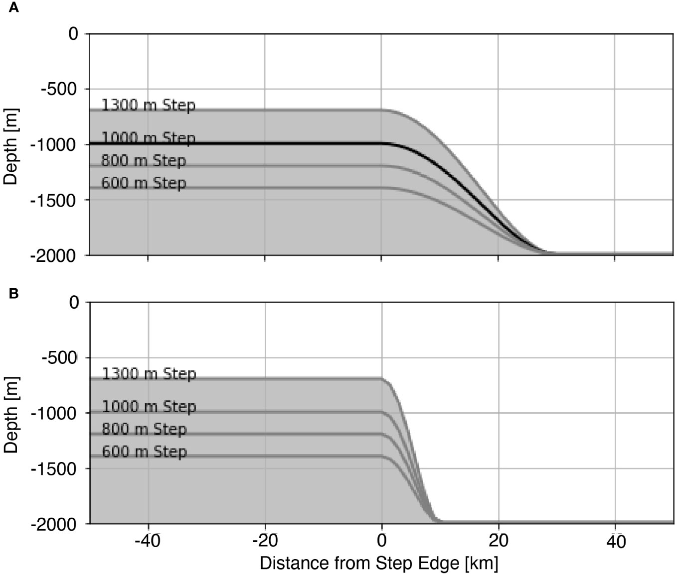
Figure 1 Step heights considered in this study with (A) subcritical and (B) supercritical slopes. The 1000 m subcritical step bathymetry discussed more extensively in the text is emphasized with a black line in (A).
The model is integrated with a 30 second time step and is forced with an idealized barotropic tide by supplying a body force to horizontal momentum equations as Bu(t) = ωU0cos(ωt) (Di Lorenzo et al. (2006)). The frequency is set as the single M2 harmonic (ω = 1/12.4 hr−1) with a maximum velocity (U0) of 0.2 m s−1. The analysis period is between the fourth and twelfth M2 cycle (days 2 - 6). Limiting the analysis period to this length prevents baroclinic energy from reentering the domain through the periodic boundaries.
We represent primary and secondary production with a simple, nitrogen-based nutrient, phytoplankton, zooplankton, detritus (NPZD) model adopted from Franks et al. (1986). The governing equations are:
In these equations, represents a Lagrangian derivative (i.e., including advective terms). This model includes vertical diffusivity for biological tracers (Kv = 10−5 m2 s−1) and neglects both sinking and horizontal mixing. The light function is represented as a simple exponential decay with depth and with constant amplitude. Though we have found our qualitative results to be insensitive to these parameters, we choose parameter values representing an oligotrophic ecosystem with small phytoplankton and small zooplankton. The nitrate half-saturation value (ks) reflects naturally occurring phytoplankton in oligotrophic environments and is 0.1 mmol N m−3 (Eppley et al. (1969); MacIsaac and Dugdale (1969)). In oligotrophic environments, grazing by small zooplankton is at a similar rate to the growth of small phytoplankton, so the zooplankton maximum grazing rate (Rm) is set to 0.4 d−1, and the maximum nutrient uptake rate (Vm) is 0.6 d−1 (Strom et al. (2006; 2007)). We assume zooplankton are inefficient consumers in oligotrophic environments by setting the grazing efficiency coefficient (γ) to 0.7 and the zooplankton excretion coefficient associated with grazing (β) to 0.15. The phytoplankton mortality rate (m), zooplankton excretion rate (Mn), and zooplankton mortality rate (Md) are all set to 0.01 d−1. Light intensity at the surface is set to one and the light attenuation coefficient (kext) is assumed to be 0.035 m−1. The level of half saturated grazing (Λ) is tuned to 0.4 mmol N m−3. Parameter values and nondimensional scaling are summarized in Table 1.
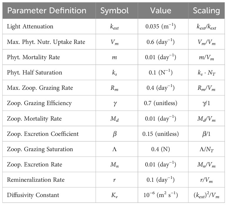
Table 1 List of parameter definitions, values, and non-dimensional scaling for the biological model.
Before coupling to the physical model, we compute a stable, vertical profile for the NPZD model initialization based on nutrient and chlorophyll concentrations measured at station ALOHA, Hawaii. Profiles of chlorophyll-a are taken from observations at station ALOHA and are converted to mmol N by assuming a C: chl-a weight ratio of 25:1 and a C:N molar ratio of 6.6:1, resulting in a conversion factor of 3.8 mmol N chl-a-1 (Karl et al. (2001); Letelier et al. (2004)). We then estimate the profile of total nitrogen (NT(z)) by assuming NT is proportional to chlorophyll-a in the upper 120 m, to average nitrate from station ALOHA between 120 m and 200 m depths, and constant below 200 m. From 65 m to 215 m depth we linearly interpolate NT from the chlorophyll-based estimate to the nitrate-based estimate to produce a smoothly varying profile. The ROMS domain is then initialized with laterally uniform profiles as calculated above and tested for further non-steady evolution. Figure 2 shows the initial profiles for the NPZD model (solid lines) and the final state (dotted) after the six-day integration in the barotropic reference domain. Field changes over 6 days are small, and much smaller than changes associated with internal tides to be studied below.
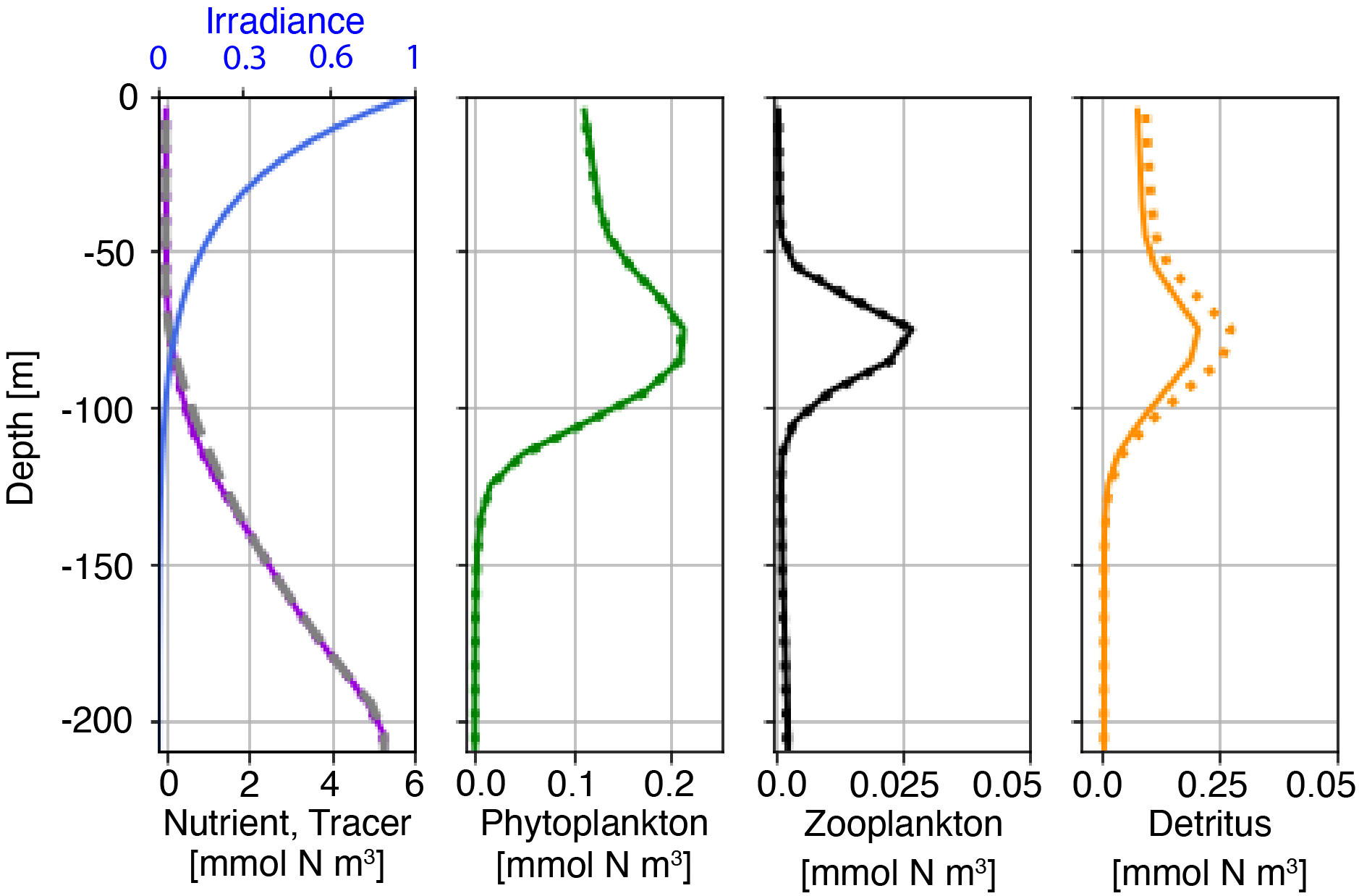
Figure 2 Initial (solid line) and final (t=6 days; dotted line) conditions for the nutrient, phytoplankton, zooplankton, and detritus concentrations. The initial profile of the nutrient-like tracer is shown as the grey dashed line and the irradiance profile is shown as the blue line in leftmost panel. Note different x-axis limits between plots.
A passive tracer is used in this study to track the redistribution of nutrients by the generation of internal tides. We initialize passive tracers with a profile resembling nutrients of the NPZD model (Figure 3, grey dashed line). We leverage the abiotic nature of the “nutrient-like” tracer, s, to determine the physical mechanisms that drive the time evolution of nutrients within the tidal beam. The budget for s can be written as:
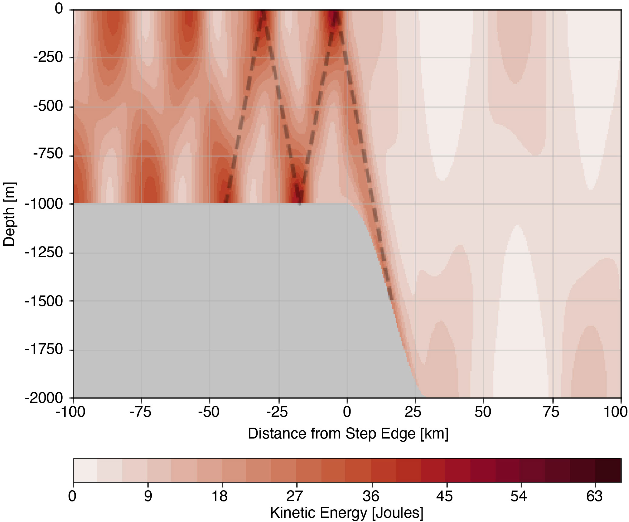
Figure 3 Average kinetic energy for the 1000 m step. The dashed line shows the first two bounces of thesubcritical tidal beam traveling along the ray path prescribed by θCg.
where u is the two-dimensional (x, z) velocity vector and Kv is the vertical diffusivity coefficient. The time-rate of change of s equals the sum of the advective flux divergence of s and its vertical diffusive flux divergence. Additionally, we capture the effect of the generation of tidal beams on nutrient redistribution by considering the average anomaly (〈s′〉) of a model simulation with a bathymetric step and internal wave generation relative to the flat bottom reference case
which is nonzero when baroclinic motions adjust the position of the nutricline relative to the barotropic reference case. A similar anomaly is computed to capture the effect of internal tide generation of primary production. In both cases, positive anomalies indicate locations where tidal beams increase the level above the barotropic reference.
Separately, Lagrangian floats track how internal tides displace water parcels containing the same NPZD model described above. Lagrangian floats are released at every horizontal grid point in each domain at the beginning of the fourth M2 cycle at 5 m increments from 5 m to 25 m depth and at 25 m increments from 25 m to 200 m depth. These Lagrangian plankton ecosystems allow us to determine the relative contributions of light and nutrient availability to primary production. We accomplish this by separating the primary production equation, see eqn. 4b, into a maximum rate Vm, light factor (), and nutrient factor ((N)/(ks + N)). Light and nutrient factors for passive plankton displaced by the internal tide are compared to those at the average depth of the orbital. Specifically, the light effect of vertical displacement by internal oscillations on primary production is obtained by defining an internal wave light factor (Lf),
that subtracts the light level at the average orbital depth from the average amount of light a (Lagrangian) passive plankton experiences over a tidal cycle. Similarly, the effect of tidal beams on nutrient availability is computed using an internal wave nutrient factor (Nf),
which measures the effect of internal wave displacement on nutrient availability relative to an unperturbed depth. Nf is the difference between the average nutrient concentration along an orbital trajectory (N(z,t)) and the initial nutrient concentration at the average depth of the orbital (N(〈z〉,t0)).
These light and nutrient factors are designed to compare the average level experienced by a passive plankton as it is displaced by the internal tide to the level experienced at the average depth of internal tide orbital. These metrics account for both the magnitude of displacement (height of the orbital) and any possible adjustment of the central position of the orbital. By separating the primary production equation in this way, we evaluate how internal tides affect light and nutrient availability for primary production, and we determine the sensitivity of each factor to bathymetric geometry.
Using the 1000 m subcritical step domain highlighted in Figure 1A as an example, we illustrate tidal beams and their effect on light and nutrient availability for primary production. As the barotropic tide encounters the step transition, energy is converted to baroclinic motion that propagates away from the step oriented along θCg in both the up- and down-range directions. Figure 3 shows the position of the subcritical tidal beam as regions of elevated average kinetic energy. As the beam propagates down range in the negative x direction, kinetic energy is largest where the beam reflects off surface and bottom boundaries, with the maximum of 48 Joules occurring at the first surface bounce. From the kinetic energy maximum, we determine the origin of the tidal beam by tracing a ray path downward along θCɡ to the mid-point of the step transition (Figure 3 dashed line). At the same time, an initially downward propagating beam reflects off the bottom boundary and propagates up-range along θCɡ. In this direction, the average kinetic energy is lower, reaching a maximum of 10 Joules. Tidal flow over a subcritical slope generates a spatially coherent up-slope traveling beam that we identify from the average kinetic energy maximum.
The effect of the generation of tidal beams on primary production is examined by considering the average anomaly of primary production (〈PP′〉) from the barotropic case. Similar to eqn. 6, 〈PP′〉 is computed by subtracting primary production in the barotropic reference case from the baroclinic experimental case such that positive values indicate locations where internal tides increase primary production. Figure 4A shows that primary production is enhanced above the barotropic reference case within the tidal beam ray path. For this 1000 m step example, the largest increase in primary production is subsurface, near the first surface bounce of the forward transmitted tidal beam and decreases at subsequent surface bounces. An example profile of average primary production (Figure 4B) outside the beam path below the red star (red line) remain qualitatively and quantitatively similar to the barotropic reference case (black dotted line). Similarly, there is relatively little change in primary production in the down-slope direction (positive x). These results suggest that primary production remains largely unaltered by the generation of the internal tides outside the beam path and that primary production is enhanced particularly within the beam path. The spatial coherence of the primary production anomaly with the position of the tidal beam motivates us to investigate whether tidal beams increase the availability of light or nutrients for primary production.
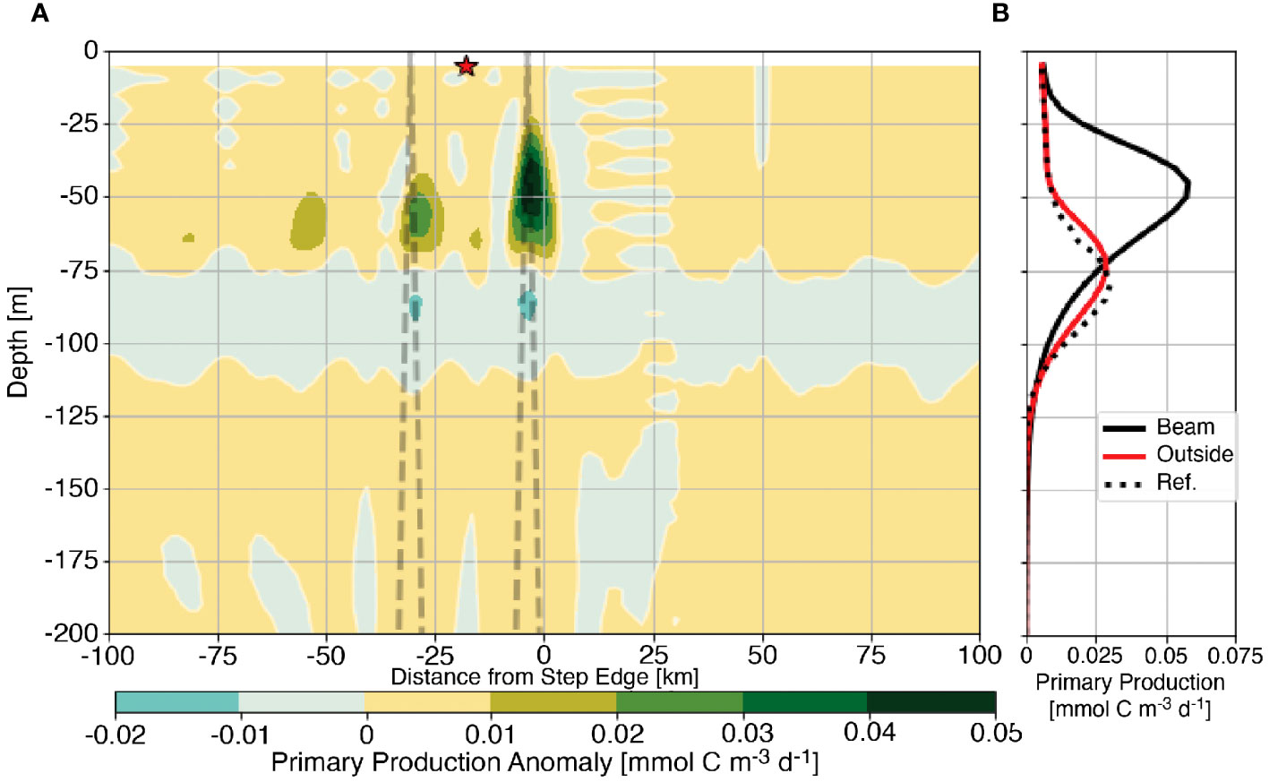
Figure 4 Primary production anomaly from the barotropic reference case for the 1000 m subcritical step with the first two bounces of the subcritical tidal beam ray path shown as the dashed line (A) Panel (B) shows average profiles of primary production from the reference case (dotted line), below the first surface bounce (solid black line), and outside of the tidal beam ray path [red line and star in (A)].
As an internal tide propagates, it oscillates passive phytoplankton vertically through varying light levels, controlling the total light available for primary production. If the light field changed linearly with depth, the light intensity increase on the upward portion of the orbital would equal the light intensity decrease on the downward portion for a symmetric orbit. However, light intensity decays exponentially with depth in the ocean (Figure 2, blue line). Phytoplankton experience more light on the upward portion of the orbital than the light lost on the downward portion, and the magnitude of vertical displacement increases the amount of light gained overall. Larger oscillations result in overall more light available for primary production.
To capture how tidal beams affect light availability for primary production, we represent passive plankton with Lagrangian floats. Floats are released throughout the euphotic zone and their position tracked over the analysis period (4th - 12th M2 cycle). The position of each float is then averaged according to the phase of the barotropic tide to produce a representative trajectory of passive plankton over a tidal cycle (Figure 5). Tidally averaged trajectories show that all orbitals orient in the direction of beam propagation (dashed line), and the vertical extent of orbitals is larger within the tidal beam than outside. Because the average light experienced by the particle is proportional to the vertical displacement, eqn. 2, phytoplankton within the tidal beam are less light-limited than those outside.
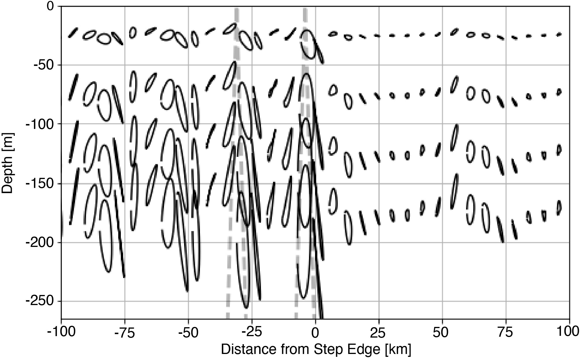
Figure 5 Tidally average Lagrangian trajectories for the 1000 m subcritical step with the position of the subcritical beam is shown as the dashed line.
The generation of internal tide beams may also affect the availability of nutrients to primary producers within the euphotic zone. In the Lagrangian frame, internal tides move nutrients with plankton into more well-lit regions. However, in the fixed (Eularian) frame, internal tides transport nutrients from deeper in the water column. To show how nutrients are affected by the generation of tidal beams in the fixed reference frame, we employ the abiotic passive tracer with an initial profile similar to the nutrient, referred to here as the “nutrient-like” tracer, s, to evaluate this possible relationship. The average anomaly of the nutrient-like tracer from the barotropic reference case (〈s′〉; eqn. 6) highlights regions where internal tides vertically redistribute nutrients (Figure 6A). The positive nutrient-like tracer anomaly within the ray path (Figure 6A dashed line) shows that tidal beams increase nutrient concentrations within the euphotic zone. The positive anomaly is largest and shallowest near the first surface bounce of the tidal beam and decreases with subsequent bounces. Profiles of the average tracer show that near the first surface bounce, tracer levels increase between approximately 30 m and 180 m depths (Figure 6B, black line). Furthermore, outside the tidal beam, the average nutrient-like tracer profile (Figure 6A red star; Figure 6B, red line) is quantitatively similar to the reference case (Figure 6B, dotted line). These results show that the effect of internal tide generation on the nutrient field is contained within the tidal beam path.
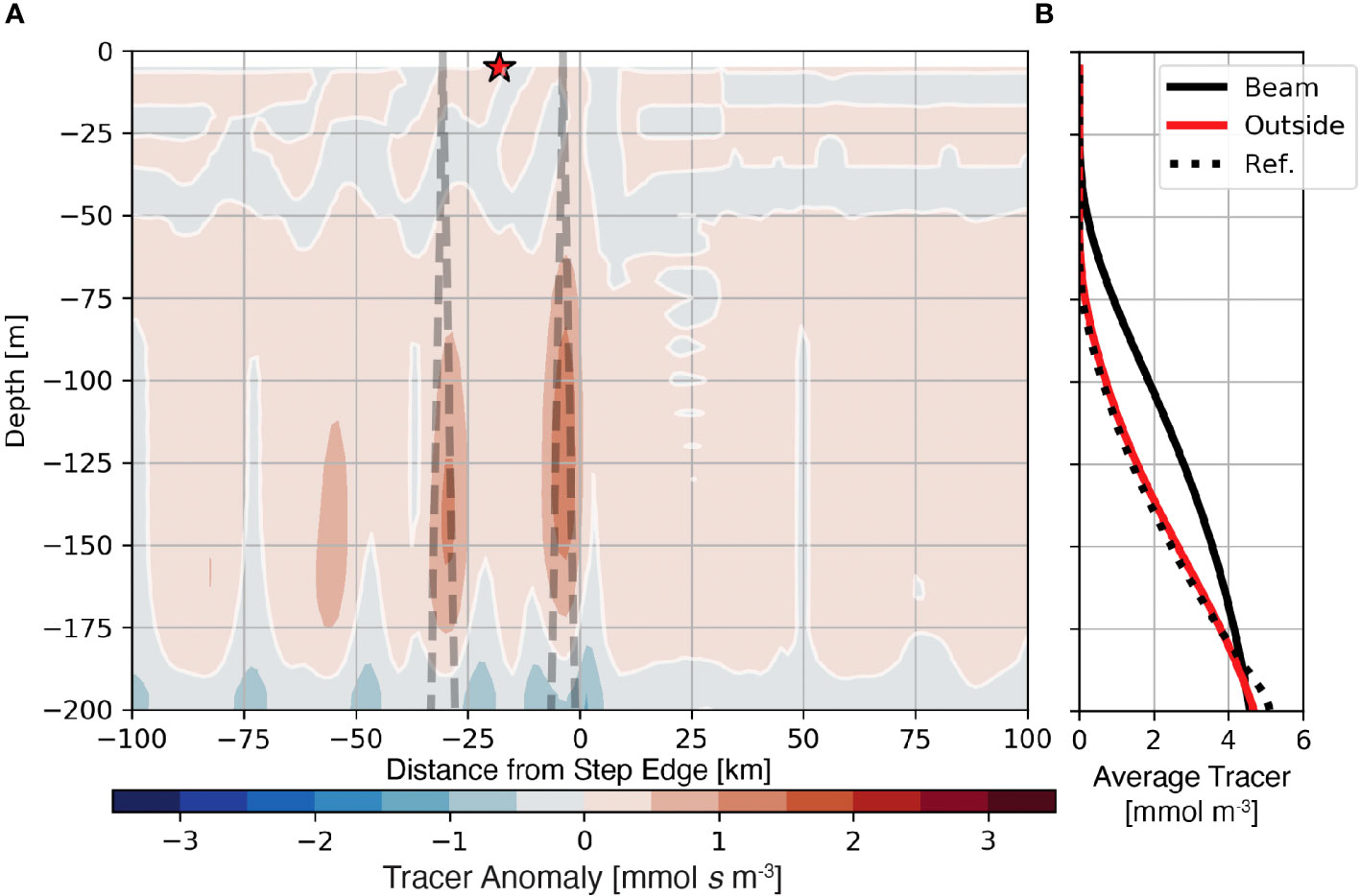
Figure 6 Nutrient-like tracer anomaly from the barotropic reference case for the 1000 m subcritical step shown with the position of the subcritical tidal beam (A). Panel (B). shows average profiles of the nutrient-like tracer from the reference case (dotted line), below the first surface bounce (solid black line), and outside of the tidal beam ray path [red line and star in (A)].
Consistent with 〈s′〉, Figure 7A shows that the time-averaged position of the tracer-cline shoals within the tidal beam ray path (dashed line). By considering the budget of s, eqn. 5, we determine the physical mechanism that drives the time evolution of the nutrients, which is controlled by either vertical mixing or advective flux divergence. The average tracer advective flux divergence (Figure 7B) shows that regions of persistent divergence (blue) and convergence (red) are oriented in the direction of the tidal beam. Within convergences, the upward flux of material is only partially compensated by horizontal fluxes, resulting in a net accumulation and an uplift of the nutricline (Figure 7A). Tidal beams adjust the position of the tracer-cline and similarly, the nutricline by creating spatially persistent regions of convergence and divergence.
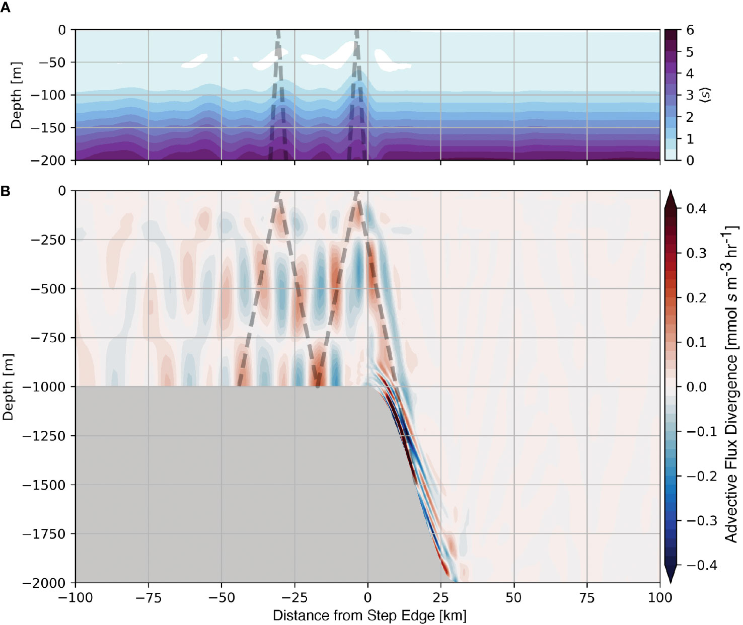
Figure 7 Average nutrient-like tracer over the 1000 m subcritical step (A) and the average advective flux divergence of the nutrient-like tracer (B). The position of the subcritical tidal beam is shown as the dashed line in both panels.
The relative scales of the advective flux divergence and mixing determine the dominant mechanism that drives the evolution of nutrients within the tidal beam. We define scales based on our numerical results as follows: U = 0.1 m s−1, W = 0.003 m s−1, L= 5000 m, H= 350 m, and Kv = 10−5 m2 s−1, for horizontal velocity, vertical velocity, horizontal length scale, vertical length scale, and diffusivity, respectively. Using these values and neglecting the arbitrary amplitude of the tracer, we find that horizontal and vertical terms within the advective flux divergence are of O(10−5 s−1; Figure 7B), whereas the diffusive flux divergence is O(10−10 s−1). This scaling analysis suggests that the advective flux divergence is several orders of magnitude larger than mixing in these idealized simulations, and our diagnostics support this conclusion. As mentioned previously, the use of an advanced mixing parameterization does not alter the contribution of mixing substantially. We note that even using Kv = 10−2 m2 s−1, which is considerably larger than typically observed near tidal beams in nature (e. g. Tuerena et al. (2019)), yields a scale for the mixing term of O(10−7 s−1), still small compared to the advective flux divergence found numerically in these experiments. Based on this scaling analysis, we argue that tidal beams locally increase the advective flux of nutrients, causing the nutricline to shoal, which fuels primary production near the base of the euphotic zone.
Adjusting the height of the subcritical step alters the kinetic energy content, depth of the nutricline, and primary production response within the tidal beam. In each of the subcritical step domains, a single forward transmitted tidal beam occurs. Near the first surface bounce of the tidal beam, average kinetic energy for the 600 m, 800 m, 1000 m, and 1300 m reaches maximum values of 25, 35, 48, and 63 Joules, respectively, indicating a linear relationship between step height (hmax) and maximum kinetic energy described by KEmax = 0.0469J m−1 · hmax(R2 = 0.9973). In response, the maximum nutrient-like tracer anomaly () increases with step height as 0.427, 0.854, 1.380, 1.763 mmol N m−3 s−1 resulting in the linear relationship described by ; (R2 = 0.9775). Similarly, the maximum primary production anomaly () increases with step height as 0.009, 0.021, 0.050, and 0.053 mmol C m−3 s−1 and results in a linear relationship described as (R2 = 0.9253). These linear correlations suggest that increases in subcritical step height proportionally raise the amount of kinetic energy in the system, resulting in greater uplift of the nutricline fueling higher rates of primary production.
In contrast to the nutricline adjustment, Lagrangian orbital trajectories within the euphotic zone respond less strongly to taller subcritical steps than deeper parcels, as they are constrained by near zero motion at the surface. While large amplitude displacements in the euphotic zone (∼ 50 m) can result in substantial changes to the light anomaly (eqn. 2) and, in turn, primary production, such displacements in the upper 100 m did not occur in our experiments. More limited displacements obtained here (⪅ 25 m) result in only weak changes in the light anomaly and thus primary production.
Bathymetry with a supercritical slope efficiently converts incoming (barotropic) tidal energy to (baroclinic) internal tides. As a result, two tidal beams emit from the critical point. We use the average kinetic energy for the 1000 m supercritical step as an example to compare these beams (Figure 8A). As the tide flows over the supercritical step, an initially Upward Propagating Beam (UPB) propagates down range, and separately, an initially Downward Propagating Beam (DPB) emits from the critical point, which then reflects off the bottom boundary before reaching the surface. The average kinetic energy within UPB is greater and more spatially coherent than the DPB, a consistent feature across the four supercritical step domains.
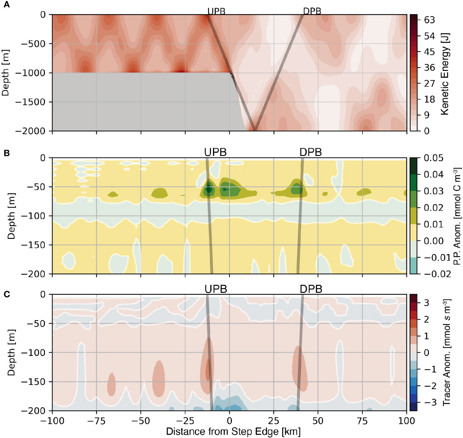
Figure 8 Average kinetic energy (A), average primary production anomaly (B), and average nutrient-like tracer anomaly (C) are shown for the 1000 m supercritical step. The positions of the initially Upward Propagating Beam (UPB) and the initially Downward Propagating Beam (DPB) are shown as the grey lines. Note the change in depth range between panel (A), and panels (B) and (C).
The regions of elevated average kinetic energy within the two tidal beams that emit from a supercritical slope affect the position of the nutricline and the level of primary production. Both UPB and DPB result in positive primary production anomalies and positive nutrient-like tracer anomalies within their respective beam paths and within similar depth ranges (Figures 8B, C), a feature that is consistent across the four supercritical step domains. However, the main difference between the two beams that emit from the critical slope is that UPB contains more kinetic energy, a larger nutrient-like tracer anomaly, and a shallower average depth of the nutricline compared to DPB. Coincident with these features is a larger maximum primary production anomaly within UPB compared to DPB. The third region of enhanced primary production located between UPB and DPB is discussed below.
Supercritical steps also differ from subcritical steps in the evolution of higher harmonics within the tidal beam. A clear way to visualize this is to compare the tidally averaged orbital trajectories from the subcritial case with the trajectories from the supercritical case. In the subcritical case (e. g. Figure 5) only the M2 harmonic exists and orbitals are roughly elliptical. In comparison, Figure 8A shows tidally averaged orbital trajectories from the supercritical case where several tidal harmonics are present. Here, an example of an M4 trajectory is highlighted in red. In this example the parcel experiencing the M4 tidal harmonic oscillates vertically twice in the time-span of one cycle for a parcel experiencing M2 fluctuations (by definition).
To ascertain the spatial distribution of tidal harmonics present within the critical case we shift from the Lagrangian frame (Figure 9A) to the fixed (Eulerian) frame (Figure 9B). At each grid cell we compute the power spectrum of vertical velocity (w) and identify the frequency with the largest power, the spectral peak. Figure 9B shows the spectral peak in each grid cell divided by the M2 frequency; near to the surface and closer to waters directly over the step transition, spectral peaks shift from the M2 frequency (1/12.4 hours; light green) to higher harmonics (darker greens) such as the M4 (1/6.2 hours), M8 (1/3.1 hours), and higher frequencies. One major consequence of the excitation of higher tidal harmonics is that tidal beam energy propagates at a steeper θCɡ (eqn. 1). The presence of several tidal harmonics greater than M2 in Figure 9B suggests that tidal beam energy is distributed over a broader region between the critical point and the first surface bounce of the M2 tidal beam.
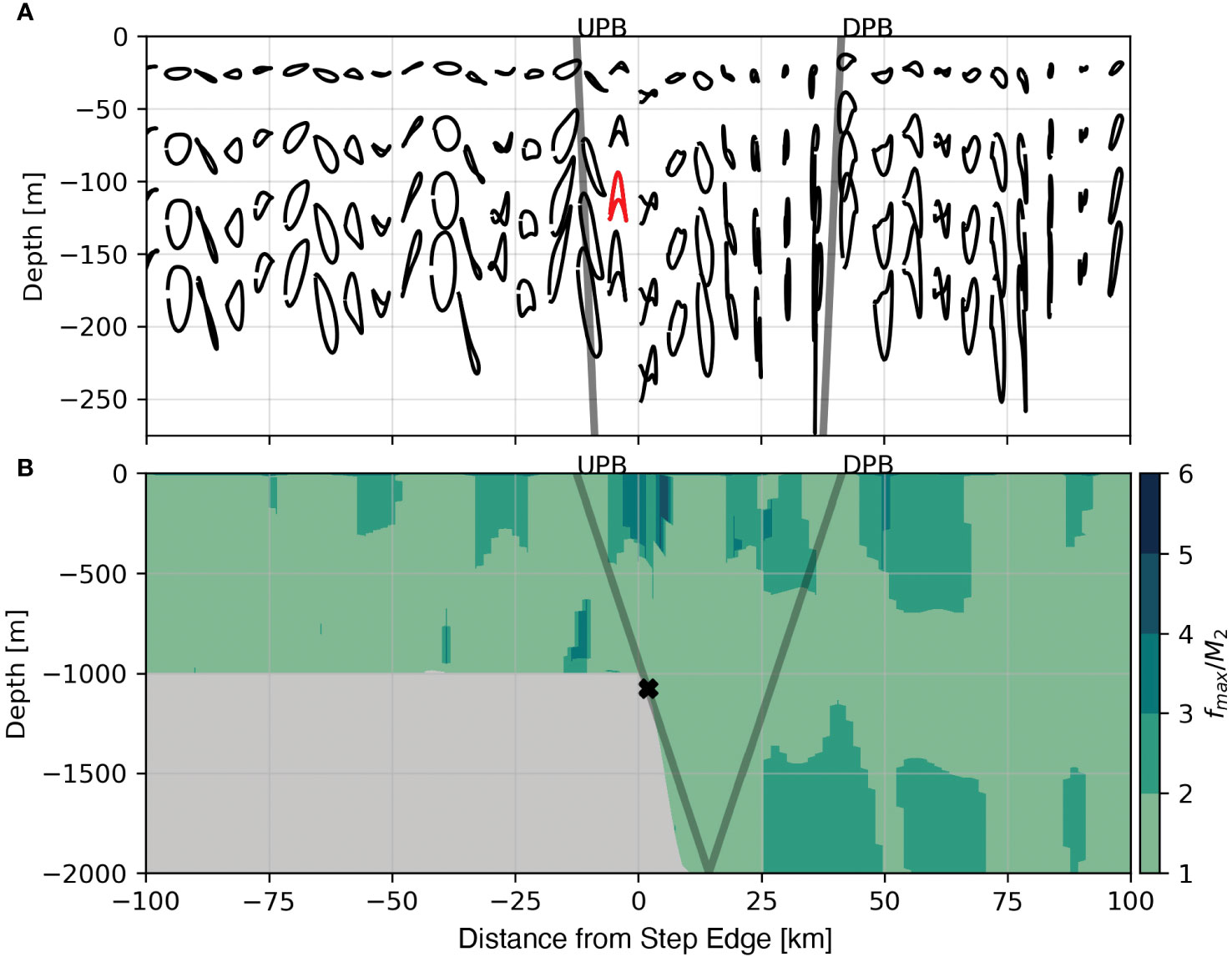
Figure 9 Tidally averaged Lagrangian trajectories for the 1000 m supercritical step with an example M4 trajectory shown in red (A) and the locations of the dominant tidal harmonic shown by dividing the frequency of the peak in spectral density by the M2 harmonic (B). The positions of the initially Upward Propagating Beam (UPB) and the initially Downward Propagating Beam (DPB) are shown as the grey lines. Note the change in depth range between panel (A) and panel (B).
The energy transfer to higher harmonics affects primary production by altering orbital trajectories and the position of the nutricline near the step transition. Regarding light availability, more frequent oscillations result in a smaller vertical displacement and thus less of a change in the average light experienced; however, the average light experienced may increase due to a shift in the average depth of an parcel. Regarding the nutricline position, the redirection of energy by the evolution of higher tidal harmonics affects the locations where the nutricline is adjusted. Figure 8C shows a small positive anomaly of the average nutrient-like tracer over the step transition indicating that the nutricline shifts to a shallower position in the same region where higher tidal harmonics are present. The net result of the redirection of energy is an increase in primary production in a broad lateral region between the critical point and the first surface bounce of the M2 tidal beam (Figure 8B).
The quantitative biological transport is sensitive to the choice of the numerical advection scheme. A comparison between upstream third order/centered fourth order (U3/C4; Shchepetkin and McWilliams (1998)) and the HSIMT (High-order Spatial Interpolation at the Middle Temporal level; Wu and Zhu (2010)) advection schemes for tracers shows a quantitative difference in tracer concentration and level of primary production. One artifact of the U3/C4 advection scheme is that advection can cause tracer concentrations to become negative (Figure 6A, white regions). In practice, negative concentrations are small and kept small owing to very small imposed reallocations within this ROMS/NPZD implementation of nitrogen from the largest biological state variable to the previously negative pool. The HSIMT scheme avoids this problem because it is positive-definite. Higher harmonic tidal beams simulated with the HSIMT scheme increase nutrient advection and subsequent primary production response relative to the more standard and widely used U3/C4 method. This result indicates uncertainty in the magnitude of the response, although both advection schemes produce the same qualitative result of increased primary production in the tidal beam paths.
We assess the relative control internal tides place on the availability of light and nutrients for primary production across the range of bathymetric step heights and slopes. In each domain, we compute primary production, the internal wave light factor (eqn. 7), and the internal wave nutrient factor (eqn. 8) for passive phytoplankton represented by Lagrangian floats initially released at 50 m depth within 50 km of the top of the step transition to focus on the first two bounces of the forward propagating tidal beam.
The Light Factor, Lf, shows that displacement through the light field results in a 2% change in primary production. The small contribution of Lf to primary production indicates that the integral of the light available over a tidal cycle changes slowly with increasing displacement caused by a more intense tidal beam. Furthermore, linear regressions show that the light factor accounts for 11.6% of the variance of primary production for supercritical steps (Figure 10A; red symbols, line), 23.9% for subcritical steps (Figure 10A; black symbols, line), and 14.1% for the combined data sets (Figure 10A; blue line). Each regression has a different slope and intercept, indicating that the relationship between primary production and Lf is sensitive to the bathymetric slope. In addition, regressions for individual domains have a wide range in slope and intercept, showing Lf is sensitive to bathymetric height. These results indicate that the change in light availability by tidal beam propagation explains a small portion of primary production and that the primary production response is decoupled from the characteristics of the tidal beam determined by the geometry of the generating bathymetry.
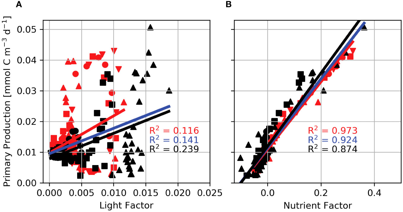
Figure 10 Internal wave Light (A) and Nutrient (B) Factors regressed against primary production for Lagrangian floats released in domains with a 600 m step (downward triangles), 800 m step (circles), 1000 m step (squares), and the 1300 m step (upward triangles). Red lines and symbols are regressions for supercritical step domains, black lines and symbols are for subcritical step domains, and the blue line is the regression for the combined data set.
In contrast, the relationship between the Nutrient Factor, Nf, and primary production shows that changes in nutrient availability result in a maximum increase in primary production by up to 38.5%. Moreover, linear regressions between the nutrient factor and primary production reveal a tight coupling between Nf and primary production (Figure 10B). Nf accounts for 97.3% of the variance in primary production for supercritical steps (Figure 10B; red symbols, red line), 87.4% for subcritical steps (Figure 10B; black symbols, lines), and 92.4% for the combined data sets (Figure 10B; blue line). The consistent slope and intercept between the three regressions suggest that the nutrient control on primary production is robust against bathymetric step height and slope. As the geometry of the bathymetry changes, so does the intensity of the tidal beam. In response, the nutrient advective flux divergence scales with w, and thus, the nutrient factor is sensitively dependent on w and tidal beam intensity.
The primary production response to tidal beam generation results from two processes (Figure 11A). First, barotropic tidal energy is converted into baroclinic energy as the tide is forced over the bathymetric step, locally displacing isopycnals vertically. The constraint on the direction of baroclinic energy propagation causes kinetic energy to localize into a tidal beam that propagates in the direction of θCg away from the step transition. The limited spatial extent of the tidal beam, combined with vertical changes in density, causes the tidal beam to generate a local advective flux divergence and a net uplift of isopycnal surfaces. In the upper region of the water column, isopycnal shoaling also carries nutrients and results in a locally shallower nutricline. Transport of nutrients vertically stimulates primary production within the tidal beam ray path.
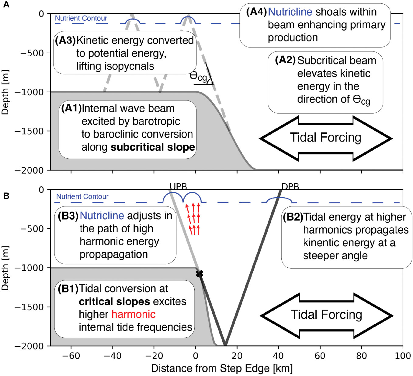
Figure 11 Conceptual models showing the processes that connect tidal beam generation to nutricline uplift over a subcritical step (A) and how multiple tidal beams affect the nutricline over topography with a critical slope (B).
The net advective flux divergence connects the position and strength of the tidal beam to the primary production response by causing the nutricline to shoal (Figures 11A, B). This mechanism explains the large correlation between the nutrient factor and primary production (Figure 10B). The kinetic energy within the tidal beam depends on the height and slope of the bathymetric step through the tidal conversion process. Therefore, the tidal conversion determines the amount of kinetic energy available for the advective flux divergence, the subsequent vertical displacement of nutrients, and the magnitude of the primary production response. The relationship between the energy content of the tidal beam and the primary production response is robust across step height and slope, indicating that nutrient enhancement has a larger effect on primary production within tidal beams.
In this work, we separate the effect of nutrient and light availability for primary production on a Lagrangian parcel by defining the Light Factor (eqn. 7) and the Nutrient Factor (eqn. 8). The Light Factor captures the transient effect of oscillation through the exponentially varying light field. Separately, the Nutrient Factor describes the time-mean effect of the tidal beam on nutrient concentrations; that is, is a continual pumping of nutrients when averaged over a tidal cycle by a net advective flux divergence within the nutricline. By decomposing the primary production equation in this way, we show that the time-dependent effect of moving through the light field has a more negligible effect on primary production than the time-averaged effect caused by the advective flux divergence of the nutrient field.
Previous work on the response of primary production to the internal waves light effect suggests that the displacement of phytoplankton through the exponentially varying light field deepens the compensation depth, increasing integrated water column productivity (Lande and Yentsch (1988); Holloway and Denman (1989); Evans et al. (2008)). The light factor presented here confirms that displacement through the light field increases primary production, but its effect is relatively small compared to the nutrient factor. In these experiments, the nutrient factor ranged from -5% to nearly 40%. A negative nutrient factor means that the displacement by internal waves reduced nutrient availability relative to a stationary position. In contrast, the light factor varied by 2%. With the bathymetric geometries test here, primary production is nearly linearly dependent on the nutrient factor. The light factor exhibited considerable scatter about a line, with low predictive skill and more considerable variability. We note that the light factor may be the dominant effect far from the generation region where the nutrient factor is negligible.
Observational and modeling studies that consider the effect of internal waves on primary production suggest that internal tides increase nutrients in the euphotic zone by elevating mixing to levels near O(10−4) (Holligan et al. (1985); Granata et al. (1995); Sharples et al. (2009); Sharples et al. (2007); Lucas et al. (2011); Stevens et al. (2012); Villamaña et al. (2017); Tuerena et al. (2019)). In the work reported here, we assumed constant vertical diffusivity of 10−5 m2 s−1. However, tests with realistic subgridscale mixing parameterizations did not show substantial changes to the mixing-induced fluxes or large quantitative changes to overall primary production in these experiments. Instead, tidal beams drive convergences in the nutrient field, increasing nutrient concentrations in the euphotic zone and stimulating primary production. Of course, divergences are also present; in these experiments, divergences occur deeper in the water column or at locations adjacent to the convergences. The divergence effect is modest due to the nutricline structure, and it is clear that the dominant factor in controlling the position of the nutricline is due to convergence.
In nature, light undergoes a diurnal light cycle that was, for reasons of simplicity, not part of our main study. The relationship between parcel orbit phase and light intensity may quantitatively impact the Light Factor. Primary production should be enhanced when the phase of the orbital displacement is shallow during daylight hours and deep at night, resulting in a higher average light along the orbital path compared to the light at the average depth. This effect would be reversed for parcels that are deep during daylight hours. We conducted a experiment identical the base case reported above but replacing exp(kextz) in eqn. 4a with A(t)exp(kextz) such that A(t) equals zero during nighttime hours and has a partial sine-wave structure during daylight. The maximum amplitude was adjusted so that the daily average light level equals one as in the constant light case. Results indicate that overall primary production is largely unchanged. The Light Factor is indeed altered by the diurnal light field, but that the Light Factor remains a small contributor to overall primary production relative to the Nutrient Factor. The Nutrient Factor is insensitive to the diurnal light field. Finally, one can imagine low-frequency beating effects that result from the difference between the 24-hour light cycle and non-daily tidal frequencies. We did not investigate this possibility because of the short duration of our experiments (7-days), necessitated by the size of our domain. We leave this potential analysis to a future study.
One critical difference between our experiments and observations in the field is that tidal beams in nature do appear to be present beyond the first surface bounce (Althaus et al. (2003); Cole et al. (2009); Rudnick (2003)). We suspect that the dissipation of the tidal beam is related to surface interactions, possibly also influenced by variable stratification in the upper ocean and near the surface. As a result, implications from this study beyond the first surface bounce should be viewed as most likely a result of the numerical configuration.
Another simplification in this study that departs from the real ocean is the prescribed linear increase of density with depth. To assess the sensitivity of this assumption, we ran an addition simulation with a realistic thermocline and a shallow mixed-layer. The base configuration of the 1000 m subcritical step was initialized with a temperature profile taken from a realistic simulation of the Hawaiian Islands domain (personal communication Tobias Friedrich). The major difference between the realistic and linear stratification cases is that the tidal beam refracts with the variable stratification, as predicted by equation 1. This refraction results in greater lateral displacement between primary productivity enhancements: the second enhancement is at x = −25 km in the base case (Figure 4A) and −100 km in the realistic stratification experiment. However, there appears to be no large impact resulting from the mixed layer, and the primary production enhancements are nearly identical in magnitude between the two stratification cases.
Global simulations of barotropic-baroclinic tidal conversion show that it is common throughout the world ocean, though some locations are more efficient at generating tidal beams than others (Simmons et al. (2004)). For example, observations over the Mid-Atlantic Ridge suggest that the tidal supply of nitrate is sufficient to sustain phytoplankton growth in the deep chlorophyll maximum in the oligotrophic gyre (Tuerena et al. (2019)). In our experiments, subcritical and supercritical slope configurations enhanced primary production relative to the reference case. Generally, taller step heights with greater associated energy conversion stimulated the largest primary production response. Based on our results, tidal beams generated by a range of bottom slopes in nature likely support ranges of primary production enhancements by aiding nutrient supply to the euphotic zone above by increasing the advective flux divergence within the nutricline.
Observational work on tidal beams consistently shows that the pycnocline shoals within the tidal beam ray path. Observations during the Hawaii Ocean Mixing Experiment (HOME) show that the mean position of isotherms is displaced toward the surface in the near-field tidal beam Cole et al. (2009). Similarly, observations of the tidal beam generated at the Mendocino Escarpment by Althaus et al. (2003) show that the tidal beam enhances the total baroclinic energy content at the base of the mixed layer which they speculate may imply a tidally driven nutrient flux. This work suggests that the mechanism through which internal tidal beams deliver nutrients to the upper ocean is due to an advective flux divergence, which causes the nutricline to shoal, increasing primary production. It may be fruitful in the future to investigate locations in nature of internal tide generation for enhanced biological response.
This study examines the primary production response to the generation of tidal beams over a range of bathymetric step heights and slopes. Larger orbital trajectories of passive plankton within tidal beams reduce subsurface light limitation, leading to higher rates of primary production. However, correlations between light enhancement and primary production in the Lagrangian reference frame suggest this is a relatively small effect. A nutrient flux convergence within tidal beams increases nutrient availability in the euphotic zone near tidal beam generation locations, fueling higher rates of primary production. Correlations between the nutrient factor and primary production indicate that nutrient supply is the larger effect of tidal beams on primary production. Because a body force generates tidal beams, they represent a mechanism that will persistently fuel primary production within the deep chlorophyll maxima, thereby contributing to the baseline level of primary production near ridges, seamounts, and escarpments throughout the global ocean.
The datasets presented in this study can be found in online repositories. The names of the repository/repositories and accession number(s) can be found below: https://oceanmodeling.ucsc.edu/projects/internal_wave_npzd/.
JJ: Conceptualization, Data curation, Formal analysis, Investigation, Methodology, Software, Validation, Visualization, Writing – original draft, Writing – review & editing. CE: Conceptualization, Funding acquisition, Methodology, Project administration, Resources, Software, Supervision, Writing – original draft, Writing – review & editing. BP: Conceptualization, Methodology, Resources, Software, Validation, Writing – review & editing. JC: Conceptualization, Methodology, Software, Validation, Writing – original draft, Writing – review & editing. JF: Methodology, Validation, Writing – review & editing.
The author(s) declare financial support was received for the research, authorship, and/or publication of this article. We gratefully acknowledge that this research was funded by the Simons Foundation through the Simons Collaboration on Computational Biogeochemical Modeling of Marine Ecosystems (CBIOMES); grant IDs: 549955 (BP) and 549949 (JRJ \& CAE).
The authors declare that the research was conducted in the absence of any commercial or financial relationships that could be construed as a potential conflict of interest.
All claims expressed in this article are solely those of the authors and do not necessarily represent those of their affiliated organizations, or those of the publisher, the editors and the reviewers. Any product that may be evaluated in this article, or claim that may be made by its manufacturer, is not guaranteed or endorsed by the publisher.
Alford M. H. (2003). Redistribution of energy available for ocean mixing by long-range propagation of internal waves. Nature 423, 159–162. doi: 10.1038/nature01628
Althaus A. M., Kunze E., Sanford T. B. (2003). Internal tide radiation from mendocino escarpment. J. Phys. Oceanography 33, 1510–1527. doi: 10.1175/1520-0485(2003)033〈1510:ITRFME〉2.0.CO;2
Balmforth N., Ierley G., Young W. (2002). Tidal conversion by subcritical topography. J. Phys. Oceanography 32, 2900–2914. doi: 10.1175/1520-0485(2002)032<2900:TCBST>2.0.CO;2
Chen Z., Xie J., Xu J., He Y., Cai S. (2017). Selection of internal wave beam directions by a geometric constraint provided by topography. Phys. Fluids 29, 066602. doi: 10.1063/1.4984245
Cole S. T., Rudnick D. L., Hodges B. A., Martin J. P. (2009). Observations of tidal internal wave beams at kauai channel, hawaii. J. Phys. Oceanography 39, 421–436. doi: 10.1175/2008JPO3937.1
Colosi J. A. (2016). Sound propagation through the stochastic ocean (New York, NY, USA: Cambridge University Press).
Cushman-Roisin B., Beckers J.-M. (2011). Introduction to geophysical fluid dynamics: Physical and numerical aspects (Waltham, MA, USA: Academic Press).
Di Lorenzo E., Young W. R., Smith S. L. (2006). Numerical and analytical estimatese of m2 tidal conversion at steep oceanic ridges. J. Phys. Oceanography 36, 1072–1084. doi: 10.1175/JPO2880.1
Dunphy M., Lamb K. G. (2014). Focusing and vertical mode scattering of the first mode internal tide by mesoscale eddy interaction. J. Geophysical Research: Oceans 119, 523–536. doi: 10.1002/2013JC009293
Eppley R. W., Rogers J. N., McCarthy J. J. (1969). Half-saturation constants for uptake of nitrate and ammonium by marine phytoplankton. Limnology Oceanography 14, 912–920. doi: 10.4319/lo.1969.14.6.0912
Evans M. A., MacIntyre S., Kling G. W. (2008). Internal wave effects on photosynthesis: Experiments, theory, and modeling. Limnology Oceanography 53, 339–353. doi: 10.4319/lo.2008.53.1.0339
Franks P. J. S., Wroblewski J. S., Flierl G. R. (1986). Behavior of a simple plankton model with food-level acclimation by herbivores. Mar. Biol. 91, 121–129. doi: 10.1007/BF00397577
Garrett C., Kunze E. (2007). Internal tide generation in the deep ocean. Annu. Rev. Fluid Mechanics 39, 57–87. doi: 10.1146/annurev.fluid.39.050905.110227
Garrett C., Munk W. (1979). Internal waves in the ocean. Annu. Rev. fluid mechanics 11, 339–369. doi: 10.1146/annurev.fl.11.010179.002011
Garwood J. C., Musgrave R. C., Lucas A. J. (2020). Life in internal waves. Oceanography 33, 38–49. doi: 10.2307/26962480
Granata T., Wiggert J., Dickey T. (1995). Trapped, near-inertial waves and enhanced chlorophyll distributions. J. Geophysical Res. 100, 20793. doi: 10.1029/95JC01665
Holligan P. M., Pingreet R. D., Mardellt G. T. (1985). Oceanic solitons, nutrient pulses and phytoplankton growth. Nature 314, 348–350. doi: 10.1038/314348a0
Holloway G., Denman K. (1989). Influence of internal waves on primary production. J. Plankton Res. 11, 409–413. doi: 10.1093/plankt/11.2.409
Karl D. M., Björkman K. M., Dore J. E., Fujieki L., Hebel D. V., Houlihan T., et al. (2001). Ecological nitrogen-to-phosphorus stoichiometry at station aloha. Deep Sea Res. Part II: Topical Stud. Oceanography 48, 1529–1566. doi: 10.1016/S0967-0645(00)00152-1
Kelly S. M., Lermusiaux P. F. (2016). Internal-tide interactions with the gulf stream and middle atlantic bight shelfbreak front. J. Geophysical Research: Oceans 121, 6271–6294. doi: 10.1002/2016JC011639
Kerry C. G., Powell B. S., Carter G. S. (2013). Effects of remote generation sites on model estimates of m2 internal tides in the philippine sea. J. Phys. Oceanography 43, 187–204. doi: 10.1175/JPO-D-12-081.1
Khatiwala S. (2003). Generation of internal tides in an ocean of finite depth: analytical and numerical calculations. Deep Sea Res. Part I: Oceanographic Res. Papers 50, 3–21. doi: 10.1016/S0967-0637(02)00132-2
Lai Z., Chen C., Beardsley R. C., Rothschild B., Tian R. (2010). Impact of high-frequency nonlinear internal waves on plankton dynamics in massachusetts bay. J. Mar. Res. 68, 259–281. doi: 10.1357/002224010793721415
Lamb K. G. (2004). Nonlinear interaction among internal wave beams generated by tidal flow over supercritical topography. Geophysical Res. Lett. 31. doi: 10.1029/2003GL019393
Lande R., Yentsch C. S. (1988). Internal waves, primary production and the compensation depth of marine phytoplankton. J. Plankton Res. 10, 565–571. doi: 10.1093/plankt/10.3.565
Large W. G., McWilliams J. C., Doney S. C. (1994). Oceanic vertical mixing: A review and a model with a nonlocal boundary layer parameterization. Rev. geophysics 32, 363–403. doi: 10.1029/94RG01872
Legg S., Huijts K. M. (2006). Preliminary simulations of internal waves and mixing generated by finite amplitude tidal flow over isolated topography. Deep Sea Res. Part II: Topical Stud. Oceanography 53, 140–156. doi: 10.1175/1520-0485(2003)033<2224:IWBACA>2.0.CO;2
Letelier R. M., Karl D. M., Abbott M. R., Bidigare R. R. (2004). Light driven seasonal patterns of chlorophyll and nitrate in the lower euphotic zone of the north pacific subtropical gyre. Limnology Oceanography 49, 508–519. doi: 10.4319/lo.2004.49.2.0508
Llewellyn Smith S. G., Young W. R. (2002). Conversion of the Barotropic tide. J. Phys. Oceanography 32, 1554–1566. doi: 10.1175/1520-0485(2002)032〈1554:COTBT〉2.0.CO;2
Lucas A. J., Franks P. J. S., Dupont C. L. (2011). Horizontal internal-tide fluxes support elevated phytoplankton productivity over the inner continental shelf: Horizontal internal-tide fluxes. Limnology Oceanography: Fluids Environments 1, 56–74. doi: 10.1215/21573698-1258185
MacIsaac J., Dugdale R. (1969). The kinetics of nitrate and ammonia uptake by natural populations of marine phytoplankton. Deep Sea Res. Oceanographic Abstracts 16, 45–57. doi: 10.1016/0011-7471(69)90049-7
MacKinnon J., Alford M. H., Sun O., Pinkel R., Zhao Z., Klymak J. (2013). Parametric subharmonic instability of the internal tide at 29 n. J. Phys. Oceanography 43, 17–28. doi: 10.1175/JPO-D-11-0108.1
Martin J. P., Rudnick D. L., Pinkel R. (2006). Spatially broad observations of internal waves in the upper ocean at the hawaiian ridge. J. Phys. Oceanography 36, 1085–1103. doi: 10.1175/JPO2881.1
Merrifield M. A., Holloway P. E. (2002). Model estimates of m2 internal tide energetics at the hawaiian ridge. J. Geophysical Research: Oceans 107, 5–1. doi: 10.1029/2001JC000996
Müller P., Holloway G., Henyey F., Pomphrey N. (1986). Nonlinear interactions among internal gravity waves. Rev. Geophysics 24, 493–536. doi: 10.1029/RG024i003p00493
Pétrélis F., Smith S. L., Young W. R. (2006). Tidal conversion at a submarine ridge. J. Phys. Oceanography 36, 1053–1071. doi: 10.1175/JPO2879.1
Pichon A., Morel Y., Baraille R., Quaresma L. (2013). Internal tide interactions in the bay of biscay: Observations and modelling. J. Mar. Syst. 109, S26–S44. doi: 10.1016/j.jmarsys.2011.07.003
Prinsenberg S., Wilmot W., Rattray M. Jr (1974). “Generation and dissipation of coastal internal tides,” in Deep Sea Research and Oceanographic Abstracts, vol. 21. (St. Frisco, CO, USA: Elsevier), 263–281.
Rainville L., Johnston T. S., Carter G. S., Merrifield M. A., Pinkel R., Worcester P. F., et al. (2010). Interference pattern and propagation of the m2 internal tide south of the hawaiian ridge. J. Phys. oceanography 40, 311–325. doi: 10.1175/2009JPO4256.1
Ray R. D., Mitchum G. T. (1996). Surface manifestation of internal tides generated near hawaii. Geophysical Res. Lett. 23, 2101–2104. doi: 10.1029/96GL02050
Rudnick D. L. (2003). From tides to mixing along the hawaiian ridge. Science 301, 355–357. doi: 10.1126/science.1085837
Sharples J., Moore C. M., Hickman A. E., Holligan P. M., Tweddle J. F., Palmer M. R., et al. (2009). Internal tidal mixing as a control on continental margin ecosystems. Geophysical Res. Lett. 36, L23603. doi: 10.1029/2009GL040683
Sharples J., Tweddle J. F., Mattias Green J. A., Palmer M. R., Kim Y.-N., Hickman A. E., et al. (2007). Spring-neap modulation of internal tide mixing and vertical nitrate fluxes at a shelf edge in summer. Limnology Oceanography 52, 1735–1747. doi: 10.4319/lo.2007.52.5.1735
Shchepetkin A. F., McWilliams J. C. (1998). Quasi-monotone advection schemes based on explicit locally adaptive dissipation. Monthly weather Rev. 126, 1541–1580. doi: 10.1175/1520-0493(1998)126<1541:QMASBO>2.0.CO;2
Shchepetkin A. F., McWilliams J. C. (2003). A method for computing horizontal pressure-gradient force in an oceanic model with a nonaligned vertical coordinate. J. Geophysical Res. 108, 3090. doi: 10.1029/2001JC001047
Shchepetkin A. F., McWilliams J. C. (2005). The regional oceanic modeling system (ROMS): a splitexplicit, free-surface, topography-following-coordinate oceanic model. Ocean Model. 9, 347–404. doi: 10.1016/j.ocemod.2004.08.002
Simmons H. L., Hallberg R. W., Arbic B. K. (2004). Internal wave generation in a global baroclinic tide model. Deep Sea Res. Part II: Topical Stud. Oceanography 51, 3043–3068. doi: 10.1016/j.dsr2.2004.09.015
Stevens C. L., Sutton P. J. H., N C. S. L. (2012). Internal waves downstream of norfolk ridge, western pacific, and their biophysical implications. Limnology Oceanography 57, 897–911. doi: 10.4319/lo.2012.57.4.0897
Strom S. L., Macri E. L., Olson M. B. (2007). Microzooplankton grazing in the coastal gulf of alaska: Variations in top-down control of phytoplankton. Limnology Oceanography 52, 1480–1494. doi: 10.4319/lo.2007.52.4.1480
Strom S. L., Olson M., Macri E., Mord C. (2006). Cross-shelf gradients in phytoplankton community structure, nutrient utilization, and growth rate in the coastal gulf of alaska. Mar. Ecol. Prog. Ser. 328, 75–92. doi: 10.3354/meps328075
Tuerena R. E., Williams R. G., Mahaffey C., Vic C., Green J. A. M., Naveira-Garabato A., et al. (2019). Internal tides drive nutrient fluxes into the deep chlorophyll maximum over mid-ocean ridges. Global Biogeochemical Cycles 33, 995–1009. doi: 10.1029/2019GB006214
Villamaña M., Mouriño-Carballido B., Marañón E., Cermeño P., Chouciño P., da Silva J. C. B., et al. (2017). Role of internal waves on mixing, nutrient supply and phytoplankton community structure during spring and neap tides in the upwelling ecosystem of ría de vigo (nw iberian peninsula): Role of internal waves in the ría de vigo. Limnology Oceanography 62, 1014–1030. doi: 10.1002/lno.10482
Warner J. C., Sherwood C. R., Arango H. G., Signell R. P. (2005). Performance of four turbulence closure models implemented using a generic length scale method. Ocean Model. 8, 81–113. doi: 10.1016/j.ocemod.2003.12.003
Waterhouse A. F., Kelly S. M., Zhao Z., MacKinnon J. A., Nash J. D., Simmons H., et al. (2018). Observations of the tasman sea internal tide beam. J. Phys. Oceanography 48, 1283–1297. doi: 10.1175/JPO-D-17-0116.1
Woodson C. (2018). The fate and impact of internal waves in nearshore ecosystems. Annu. Rev. Mar. Sci. 10, 421–441. doi: 10.1146/annurev-marine-121916-063619
Wu H., Zhu J. (2010). Advection scheme with 3rd high-order spatial interpolation at the middle temporal level and its application to saltwater intrusion in the changjiang estuary. Ocean Model. 33, 33–51. doi: 10.1016/j.ocemod.2009.12.001
Keywords: primary production, internal tides, tidal beams, nutricline uplift, idealized numerical modeling
Citation: Jacobsen JR, Edwards CA, Powell BS, Colosi JA and Fiechter J (2023) Nutricline adjustment by internal tidal beam generation enhances primary production in idealized numerical models. Front. Mar. Sci. 10:1309011. doi: 10.3389/fmars.2023.1309011
Received: 07 October 2023; Accepted: 24 November 2023;
Published: 14 December 2023.
Edited by:
Wen-Zhou Zhang, Xiamen University, ChinaReviewed by:
Zhiwei Zhang, Ocean University of China, ChinaCopyright © 2023 Jacobsen, Edwards, Powell, Colosi and Fiechter. This is an open-access article distributed under the terms of the Creative Commons Attribution License (CC BY). The use, distribution or reproduction in other forums is permitted, provided the original author(s) and the copyright owner(s) are credited and that the original publication in this journal is cited, in accordance with accepted academic practice. No use, distribution or reproduction is permitted which does not comply with these terms.
*Correspondence: Jasen R. Jacobsen, amphY29iczJAdWNzYy5lZHU=
Disclaimer: All claims expressed in this article are solely those of the authors and do not necessarily represent those of their affiliated organizations, or those of the publisher, the editors and the reviewers. Any product that may be evaluated in this article or claim that may be made by its manufacturer is not guaranteed or endorsed by the publisher.
Research integrity at Frontiers
Learn more about the work of our research integrity team to safeguard the quality of each article we publish.