 Wenxin Xie
 Yong Li1*
 Zhaoxuan Li
 Qiang Mei
94% of researchers rate our articles as excellent or good
Learn more about the work of our research integrity team to safeguard the quality of each article we publish.
Find out more
ORIGINAL RESEARCH article
Front. Mar. Sci., 01 December 2023
Sec. Marine Pollution
Volume 10 - 2023 | https://doi.org/10.3389/fmars.2023.1308981
The escalating greenhouse gas (GHG) emissions from maritime trade present a serious environmental and biological threat. With increasing emission reduction initiatives, such as the European Union’s incorporation of the maritime sector into the emissions trading system, both challenges and opportunities emerge for maritime transport and associated industries. To address these concerns, this study presents a model specifically designed for estimating and projecting the spatiotemporal GHG emission inventory of ships, particularly when dealing with incomplete automatic identification system datasets. In the computational aspect of the model, various data processing techniques are employed to rectify inaccuracies arising from incomplete or erroneous AIS data, including big data cleaning, ship trajectory aggregation, multi-source spatiotemporal data fusion and missing data complementation. Utilizing a bottom-up ship dynamic approach, the model generates a high-resolution GHG emission inventory. This inventory contains key attributes such as the types of ships emitting GHGs, the locations of these emissions, the time periods during which emissions occur, and emissions. For predictive analytics, the model utilizes temporal fusion transformers equipped with the attention mechanism to accurately forecast the critical emission parameters, including emission locations, time frames, and quantities. Focusing on the sea area around Tianjin port—a region characterized by high shipping activity—this study achieves fine-grained emission source tracking via detailed emission inventory calculations. Moreover, the prediction model achieves a promising loss function of approximately 0.15 under the optimal parameter configuration, obtaining a better result than recurrent neural network (RNN) and long short-term memory network (LSTM) in the comparative experiments. The proposed method allows for a comprehensive understanding of emission patterns across diverse vessel types under various operational conditions. Coupled with the prediction results, the study offers valuable theoretical and data-driven support for formulating emission reduction strategies and optimizing resource allocation, thereby contributing to sustainable maritime transformation.
Over recent decades, the increasing seaborne trade has mirrored a corresponding increase in greenhouse gas (GHG) emissions from maritime vessels. According to the fourth GHG report released by the International Maritime Organization (IMO) in 2021, The GHG emissions—including carbon dioxide (CO2), methane (CH4) and nitrous oxide (N2O), expressed in CO2e—of total shipping (international, domestic, and fishing) have increased from 977 million tonnes in 2012 to 1,076 million tonnes in 2018 (9.6% increase). This increase amplified the shipping sector’s contribution to global anthropogenic emissions from 2.76% in 2012 to 2.89% in 2018. Alarmingly, these emissions are set to escalate further, with forecasts suggesting an increase from 1,000 Mt CO2 in 2018 to 1,500 Mt CO2 by 2050 (IMO, 2021).
The upward trajectory of GHG emissions has caused substantial disruptions in the global climate, exemplified by exacerbated global warming. Such warming diminishes terrestrial and aquatic carbon sinks, resulting in a larger fraction of anthropogenic emissions remaining in the atmosphere. This mechanism amplifies the atmospheric CO2 concentration, leading to more significant climatic alterations. The consequences of climatic alterations are broad and irreversible. For instance, if global temperatures surpass the 1.5 to 2.5°C threshold above the 1980–1999 baseline, an endangerment of 20% to 30% of evaluated species is probable (IPCC, 2007). Moreover, climate-induced transformations permeate atmospheric, aquatic, glacial, and biological spheres, inflicting profound damage. For example, the global sea level has risen by 0.2 meters from 1901 to 2018. As these levels elevate, heightened climatic extremes, threaten both natural ecosystems and human settlements (IPCC, 2023). The pressure for air pollution control is also increasing due to its detrimental effects on marine environments and human health (Zhou and Leng, 2021).
Addressing the environmental concerns posed by the maritime sector, there has been an increase in emission reduction policies. The IMO established the International Convention for the Prevention of Pollution from Ships (MARPOL Convention) aimed at mitigating pollution from ships. More recently, On February 8-9, 2023, the Committee of Permanent Delegations to the Council of the European Union (EU Council) and the Committee on the Environment of the European Parliament (EP) respectively endorsed the emissions trading system (ETS). The revised final compromise text regarding the inclusion of the maritime sector in the EU ETS details the timetable, navigational emission coverage, applicable ship tonnage, emission coverage, and fund utilization. The drive for maritime emission reductions resonates globally, not just within the EU. However, the endeavor to integrate the maritime domain within the ETS, aimed at energy conservation and emission reductions, is complex. Addressing the diverse challenges and leveraging emerging opportunities requires timely and rigorous explorations.
Recent academic efforts have shed light on shipborne carbon mitigation strategies. Among the well-explored interventions are ship speed adjustments, coastal electrification, and the transition towards cleaner fuel alternatives (Zhou and Leng, 2021). Studies have shown that slowing down vessel speeds can effectively reduce immediate CO2 emissions (Cariou, 2011). Various alternative energy solutions—encompassing fuel cells, waste heat recovery, solar and wind energy utilization, shore electrification, and cleaner fuels—demonstrate theoretical promise (Wan et al., 2018).
However, there are many factors playing a role in influencing pollutant emissions, such as shipper preferences, societal responsibility, and government policies. It is acknowledged that no single technology provides comprehensive mitigation across all sectors. Although various studies have addressed the issue of carbon emission reduction from ships from different perspectives, the comprehensive carbon emission reduction pathway in the shipping industry often lack clear scientific guidelines. The development of scientifically based and targeted emission reduction measures is a key issue. This calls for a comprehensive understanding, not only of cumulative emissions but also their origins, including areas of carbon emission hotspot and vessel-specific attributes. Such insights will enable stakeholders and policymakers to craft informed policies (Zhou et al., 2023).
Comprehensive emission inventories encompass both emission sources and pollutant categories. Reliable inventories are fundamental to policy formation and subsequent efficacy evaluations in air pollution management (He et al., 2021). In maritime pollution studies, emission inventory methodologies often stand out as the most practical source analysis technique (Xie, 2020). Present maritime emission characterizations heavily rely on these inventories, with predominant methods comprising top-down calculations based on ship fuel consumption (Hulskotte and Denier van der Gon, 2009) and bottom-up methodologies utilizing the automatic identification system (AIS) (Johansson et al., 2017; Chen et al., 2018; Mao et al., 2020; Gan et al., 2022).
The accuracy of the fuel consumption method in estimating emissions is yet to be proved due to factors such as deviations in fuel consumption and emission factors. The dynamic method based on AIS, categorizes emissions based on the ship’s different sailing states and type, offering superior spatiotemporal granularity. Due to the widespread adoption of modern navigation information systems, AIS has evolved into an indispensable tool, providing real-time, global insights into ship operations (Mou et al., 2019). The frequency of transmission of AIS data enables ships to obtain multiple AIS data records from other ships in a short period of time (Weng et al., 2019). Such accuracy ensures emissions can be pinpointed with remarkable precision using AIS datasets.
Ship emission inventories inherently display temporal sequencing, categorizing them as time-series data. This type of data, rich in temporal details, facilitates the mining of patterns and trends across time. By leveraging historical data, one can forecast the future trajectory of a time-series variable. Such forecasts are essential across various real-world applications with temporal details, including meteorology, energy consumption, financial forecasting, medical surveillance, anomaly detection, industrial production, sales, and traffic predictions. As the volume and dimensionality of time-series data have expanded, the methodologies for time series forecasting (TSF) have seen continuous refinement (Mao et al., 2023). The evolution has transitioned from initial mathematical-statistical methods to machine learning techniques, eventually embracing deep learning strategies.
Before data mining gained prominence, traditional TSF predominantly employed statistical models. Pioneering models included the autoregressive (AR) model (Yule, 1927), the moving average (MA) model (Slutzky, 1937), the autoregressive moving average (ARMA) model (Kendall and Wold, 1954), and the autoregressive integrated moving average model (ARIMA) (Zhang, 2003). Additional methodologies like Holt’s linear trend and Holt-Winters (Chatfield, 1978) also emerged. Rooted in linear functions derived from recent observations, these models have seen extensive application across various forecasting challenges. However, their efficacy diminishes when dealing with non-smooth, intricate real-world time series, as they often overlook the demands of smoothness and ergodicity (Lara-Benıtíez et al., 2021).
With the advent of machine learning, predictive models such as support vector machine (SVM) (Cortes and Vapnik, 1995), support vector regression (SVR) (Chen et al., 2013), Bayesian network (Das and Ghosh, 2015), Gaussian process (GP) (Rasmussen, 2004), and random forest (RF) (Breiman, 2001) began to outperform traditional statistical counterparts (Chen, 2021). Machine learning’s innate ability in nonlinear modeling and generalization has substantially strengthened prediction accuracy. However, one notable limitation is their feature-centric modeling approach, which often neglects the intrinsic temporal dependencies inherent in time-series data (Tan, 2020).
Neural networks, illustrating a potent nonlinear model, are celebrated for their robust capability. Among the neural networks tailored for time-series data prediction, the back-propagation (BP) neural network stands out as a widely adopted model (Wang et al., 2011). Multilayer perceptron (MLP) has also demonstrated efficacy in time-series prediction tasks (Zhang et al., 1998; Zhang, 2003). Though these feedforward neural networks have been successfully deployed across various scenarios, their architecture inherently processes each input in isolation. This renders them inept at capturing the sequential complexities embedded within time-series datasets. This limitation can compromise their efficacy in TSF, especially when grappling with dynamic datasets of varying lengths (Lara-Benıtíez et al., 2021).
The ubiquity of Internet of Things (IoT) sensors has introduced an era where large amounts of time-series data are constantly generated across diverse scientific fields. This relentless data generation has posed challenges for traditional parametric models and machine learning algorithms in efficiently processing this time-series data. Consequently, leveraging deep learning algorithms to extract valuable insights from time-series data has captured the interest of numerous researchers (Liang et al., 2023). Deep learning excels in extracting both linear and nonlinear features, identifying patterns often elusive to shallower neural networks. Convolutional neural network (CNNs) (Li et al., 2017), recurrent neural network (RNNs) (Schuster and Paliwal, 1997; Goodfellow et al., 2016), and transformer-based models (Vaswani et al., 2017; Wen et al., 2022) have made notable advancements in time-series prediction, consistently delivering commendable results. The bidirectional encoder representation from transformers (BERT) model (Devlin et al., 2018) in time-series prediction tasks also overcomes the problem of scenario application limitations (Jin et al., 2021). The adversarial sparse transformer (AST) proposed in 2020 addresses the prediction model’s inability to deal with real stochasticity in time-series problems (Wu et al., 2020). Informer (Zhou et al., 2020), TFT (Lim et al., 2021), SSDNet (Lin et al., 2021), Autoformer (Wu et al., 2021), Aliformer (Qi et al., 2021), FEDformer (Zhou et al., 2022), and other models based on the attention mechanism have all achieved superior results on temporal prediction tasks.
Given the existing challenges in the shipping industry and the current state of relevant research, this paper developes a robust spatiotemporal GHG emission inventory estimation and prediction model capable of handling incomplete AIS datasets through the dynamic method and the Temporal Fusion Transformers (Lim et al., 2021) with attention mechanism.We integrate AIS data, Lloyd’s ship data, and geographic information. The potential inaccuracies resulting from missing or erroneous AIS data have been mitigated using data preprocessing techniques. These include big data cleaning, ship trajectory aggregation, multi-source spatiotemporal data fusion and missing data complementation.
Using the shipping activities in the sea area of Tianjin Port in 2018 as a case study, this paper achieves high-resolution estimation and forecasting of the spatiotemporal emission inventory of GHGs from vessels. Emphasizing the emission characteristics of various ship types under different operational conditions, and the multitude of factors that might influence ships’ GHG emissions, this study offers an intricate breakdown of emissions. This granularity extends to each individual ship and port equipment, enhancing data-driven strategies for carbon trading and optimizing port resource allocation. For clarity, ship categories include dry bulk carriers, container ships, oil tankers, fishing vessels, general cargo ships, ro-ro ships, cruise ships, tugboats, car carriers, among others. Ship operational states are classified as cruising, low speed sailing, harbor maneuvering, anchoring, and berthing. Additionally, emissions are quantified by the main engine (ME), auxiliary engine (AE), and boiler.By predicting GHG emissions, emission timelines, and pinpointing emission sources, this research provides data and theoretical insights that empower relevant stakeholders to formulate specific emission reduction strategies and controls.
The subsequent section of this article delves into the research subject, elucidates the computation and prediction models, followed by an analysis of the model results and policy recommendations from various perspectives. The final section ends with the study’s conclusions and discussions.
Utilizing the sea area of Tianjin Port as a case study, this paper leverages the 2018 AIS data, ship Lloyd’s file data, and geographic information of Tianjin Port to formulate a high-resolution ship GHG emission inventory and predicts the characteristics of ship GHG emissions.
Research indicates that approximately 70% of ship emissions occur within 400 kilometers of land (Endresen and Sorgard, 2003). In China, emissions from domestic emission control areas (DECAs) within 12 nautical miles contribute to around 40% of total ship emissions along its coasts, a figure that doubles when the DECA boundary extends to 100 nautical miles. Ports are significant emission sources, accounting for about a quarter of total emissions within 200 nautical miles, with nearly 80% of these emissions concentrated in China’s ten busiest ports (Li et al., 2018). The surge in international trade and corresponding shipping activities has exacerbated the environmental impact of ship emissions. Studies reveal that sea winds can carry ship emissions from sea to land, contributing to environmental pollution in coastal cities (Liu et al., 2017). Moreover, heavy ship traffic is linked to deteriorated air quality in port areas (Ng et al., 2013; Li et al., 2016; Weng and Li, 2019), posing adverse effects on both global climate and human health (IPCC, 2007; Corbett et al., 2007).
Tianjin Port, situated in the Binhai New Area of Tianjin City, is a crucial hub for China’s foreign trade and the entry of foreign materials and equipment into the country. With a container throughput surpassing 20 million TEUs in 2021, it ranks eighth worldwide (Wang, 2022), serving as the most important comprehensive hub port in northern China and the world’s largest man-made deep-water port (Niu, 2022). Tianjin Port, a hub of bustling international trade, witnesses a significant influx and outflux of international vessels. While this trade dynamic propels economic growth, it simultaneously imposes significant environmental responsibilities on local authorities to mitigate pollution. The drive for green transformation, although promising, presents a multitude of challenges.
Among the global shift towards sustainable development, the implementation of emission reduction policies is on the rise. An exemplary policy is the integration of maritime activities into the EU ETS. Such policies, while presenting opportunities for various sectors, also pose significant challenges to the global shipping industry. Navigating these evolving international policies and regulations will be crucial for the survival and growth of the shipping sector. For instance, the EU ETS mandates entities associated with ships—be it shipowners, management entities, or charterers—to bear the costs for the GHGs their vessels emit during voyages to, within, and from EU ports. Furthermore, from 2026, the regulatory scope will expand to encompass emissions like CO2, N2O, and CH4. Given this backdrop, it is necessary for the global shipping industry to proactively strategize. This entails anticipating potential policy shifts, rigorously monitoring a broader spectrum of pollutant emissions, evaluating the climate impacts of diverse GHGs emitted by maritime activities, and identifying novel avenues of opportunity in emerging green pathways.
This research delves into a comprehensive analysis of GHG emissions from ships operating in Tianjin Port. The scope of the study spans across seven channels, eight anchorages, and 205 berths, meticulously evaluating the emissions of CO2, N2O, and CH4. The goal is to provide data-backed insights for authorities to implement effective, targeted policies for emission reduction, aligning with green transition initiatives.
The research employs data from the AIS and specifically selects the AIS data pertaining to Tianjin Port from the year 2018, alongside the ship archive from Lloyd’s data, and geographic information about Tianjin Port.
AIS, being a navigational aid, furnishes extensive information about ships and is revered as a dependable data source, significantly diminishing uncertainties surrounding ship activities and their geographic dispersion (Wang et al., 2008; Dalsøren et al., 2009; Bandemehr et al., 2015). The AIS system transmits signals at intervals ranging from every three seconds to a few minutes, showcasing detailed insights into a ship’s speed and location. The brief transmission time of AIS data facilitates the acquisition of multiple AIS records for a ship within a compact time frame (Weng et al., 2019). Even at a distance not exceeding one kilometer, ship emissions can be calculated at least once, even if the ship is moving at a high velocity (Chen et al., 2017), ensuring the precise computation of ship emissions. Figure 1 illustrates the distribution of ship trajectories within Tianjin Port waters for the study area in 2018.
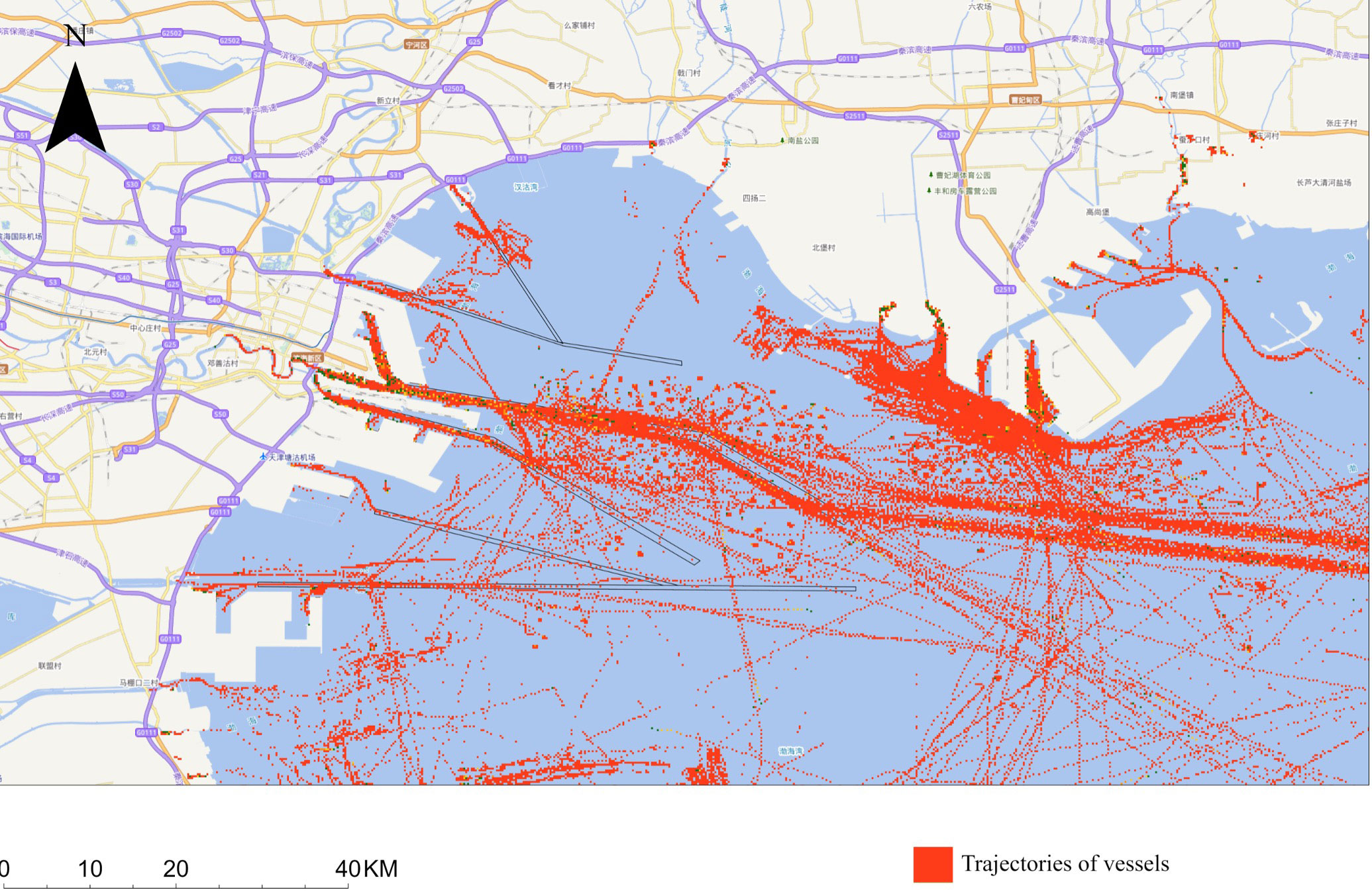
Figure 1 Tianjin Port Waters and Distribution Map of Ship Trajectories in 2018.
Ship identification leverages the maritime mobile service identity (MMSI) code provided in AIS data, with each ship possessing a unique MMSI code. The AIS data include a diverse array of information, segmented into static information, dynamic information, voyage-related information, and safety-related short messages. Static information encompasses the vessel’s MMSI number, vessel name, vessel type, dimensions (length and breadth), tonnage, and the country of registration. Conversely, dynamic information includes the ship’s positional coordinates (longitude and latitude), heading, velocity, and timestamp (UTC seconds, indicating the time of report generation).
The Lloyd’s vessel file houses fundamental information about the vessel, such as MMSI, vessel type, country and region of registration, tonnage, design speed, main engine’s maximum continuous power, auxiliary engines’ power, main engine’s rotational speed (RPM), construction year, fuel oil type, vessel maneuvering unit, vessel registration ownership unit, vessel management unit, and a detailed description of the vessel’s capacity.
For the purposes of this study, ships are classified into categories such as dry bulk carriers, container ships, oil and chemical tankers, ro-ro ships, fishing vessels, cruise ships, general cargo ships, tugs, and others to facilitate a thorough analysis of pollutants.
AIS data contain extensive maritime information, which can be extracted to illuminate insights on a vessel’s navigational status. This data is indispensable across a wide range of marine applications including collision avoidance, marine surveillance, trajectory clustering (Xiao et al., 2015), maritime traffic forecasting, and accident investigations. Nevertheless, the AIS data acquisition lifecycle—spanning generation, encapsulation, transmission to reception, and decoding—is prone to data gaps, inaccuracies, duplications, and other issues due to factors such as AIS signal propagation anomalies and equipment malfunctions (Zhao et al., 2014; Zhao et al., 2015; Wei and Yang, 2016; Wu et al., 2017). The challenge intensifies when attempting to integrate AIS data with the Lloyd’s ship database, where discrepancies like unmatched vessel entries between the AIS dataset and the Lloyd’s database or incomplete entries within the Lloyd’s database are frequent.
Given the pivotal role of the ship emission inventory in mitigating pollution and promoting maritime environmental stewardship, rigorous preprocessing of the raw AIS data is imperative. This entails a series of operations including data cleansing, trajectory consolidation, data fusion, and data supplementation, each crucial for ensuring the data’s integrity, accuracy, and reliability, thus setting a solid groundwork for accurate subsequent analyses. The step-by-step procedure of AIS data preprocessing is visually depicted in Figure 2.
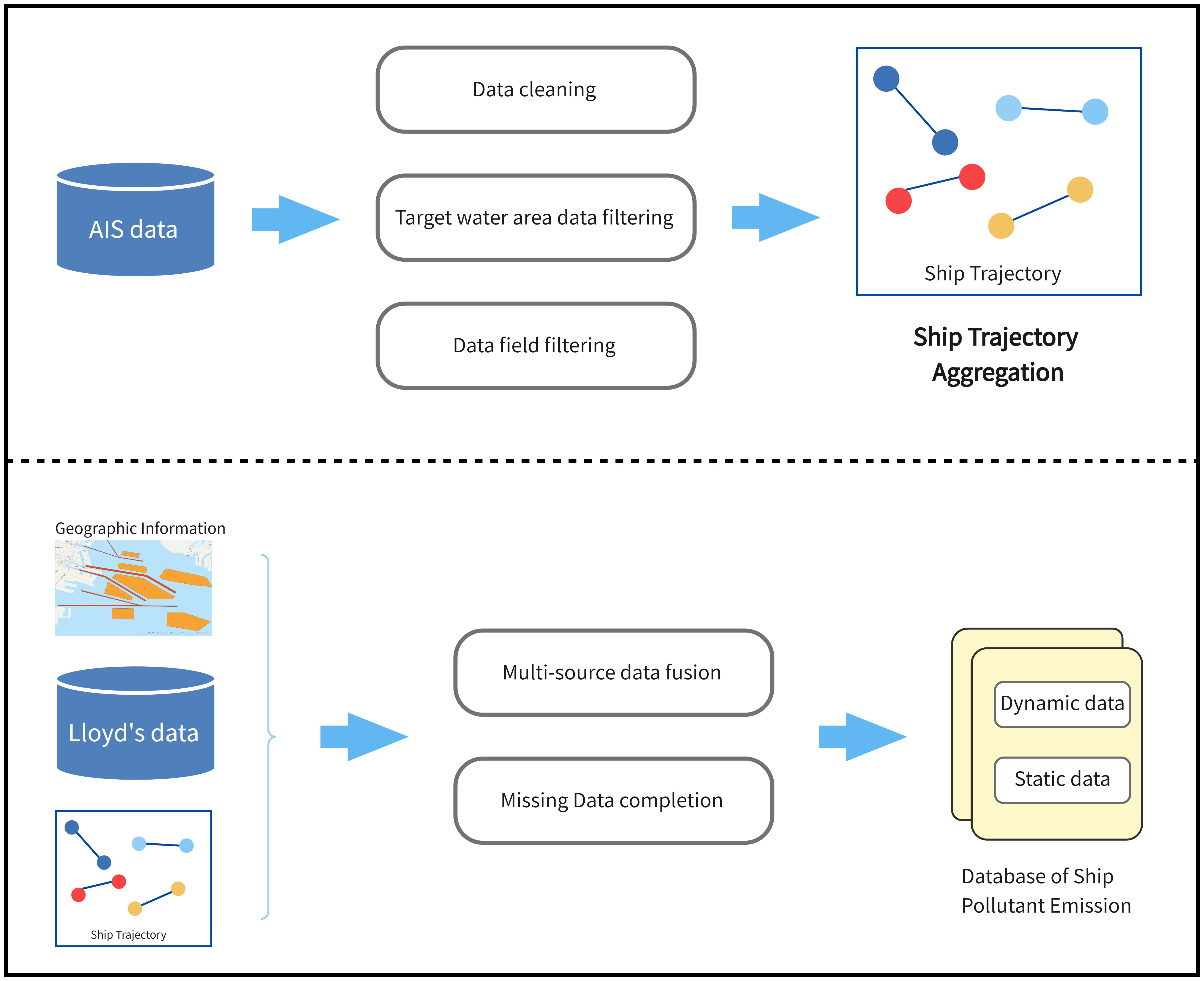
Figure 2 Workflow of AIS Data Preprocessing.
Given its frequent broadcasting intervals for navigating ships coupled with a dense ship presence in harbor waters, the amount of AIS data is substantial. For instance, in the waters around Xiamen harbor, daily AIS data influx exceeds 400,000 records (Pan, 2015). Marine traffic studies often demand data spanning over extensive periods, such as quarters or entire years. Efficiently extracting useful insights from this deluge of AIS data has consequently emerged as a focal research area in maritime transportation science (Shao et al., 2007).
The range of very high frequency (VHF) radio signals transmitted by AIS-equipped vessels on the Earth’s surface is finite. Detailed tracking of vessels around coastal areas necessitates an adequate density of ground stations. For remote areas beyond these ground stations, satellite AIS collection is pivotal but can be compromised by signal collisions (Goldsworthy, 2017).
Given potential inconsistencies during AIS equipment usage, data transmission, collection, and data management phases, raw AIS data often teem with missing entries, errors, duplicates, and other anomalies. These discrepancies can muddle subsequent analyses, thus necessitating rigorous data cleaning tailored to this study’s specific needs-calculating and predicting ship-related GHG emissions (Pan et al., 2010; Zhu et al., 2012).
We undertook the following data cleaning and validation steps based on the raw AIS data (Xiao et al., 2015):
● Speed validation: AIS records indicating real-time ship speeds surpassing their design speeds were flagged as anomalies, resulting in the deletion of such data points.
● Position verification: Data points showing vessel positions outside the Tianjin Port waters or landmasses were deemed erroneous and purged.
● Heading angle filter: Vessel heading angles typically range between 0 to 360 degrees. Any deviations from this range prompted data point removal.
● Time validation: Data entries with anomalous timestamps or those falling outside the research time frame were categorized as time-based anomalies and discarded.
● MMSI verification: MMSI, consisting of 9 digits, along with other data fields such as IMO, latitude, and longitude, was assessed against threshold values. Data points exceeding these thresholds were excluded.
● De-duplication: Based on unique identifiers such as the vessel’s IMO number, MMSI number, vessel name, and data transmission timestamp, duplicate entries were identified and removed.
Post-cleaning, relevant data fields—covering aspects like location, MMSI, timestamp, speed, vessel type, nationality, tonnage, and other vessel attributes—were filtered out and imported into a database for subsequent processing and analysis.
The frequency with which ships transmit AIS signals while sailing varies between every 3 seconds to several minutes. Given the high volume of vessels in port waters, Tianjin Port’s 2018 AIS data accumulation is substantial, making direct usage for subsequent analyses resource-intensive. Moreover, the AIS data transmission intervals are significantly more frequent than the time frames required for ship emission calculations (Goldsworthy, 2017). Therefore, it is imperative to integrate this vast expanse of AIS data, pinpointing key nodes that best describe the original trajectory from densely sampled points. These nodes, when chronologically linked, yield the ship’s complete navigational route within Tianjin Port. Given the high density of these point data, the extracted trajectories undergo compression to simplify subsequent computations and better capture primary navigational features (Wang and Li, 2021).
In our methodology, we filtered out AIS data track points based on a ship’s MMSI where the latitude and longitude intersect with the vectors of port facilities (e.g., channels, anchorages, berths). After chronologically organizing these track points by their sampling timestamps, the vessel’s navigational trajectories were generated. Concurrently, we computed the time difference between route entries and exits, averaging the travel speed of each trajectory point, culminating in an average velocity for the entire navigational route. This approach ensures efficient data extraction from the vast primary AIS datasets for ensuing computations.
Our statistical analysis on maritime operations within Tianjin Port indicates standard dwell times: a vessel usually spends no more than 4 days at a berth, 20 days in anchorage, and 2 hours navigating the channel. Any ship exceeding these time frames is flagged for trajectory anomalies and consequently omitted from the dataset.
The computation of ships’ GHG emission inventories and the subsequent emission characteristic analyses require more than merely the static and dynamic AIS data. They call for the incorporation of vessel attribute information from the Lloyd’s Register of Ships and relevant geographical data regarding port facilities. This study achieves the integration of this multi-source spatiotemporal data—encompassing AIS data, Lloyd’s Register data, and geographic details—by utilizing spatial computation and database technology.
Developing a comprehensive ship emission estimation methodology capable of handling incomplete AIS datasets is crucial to maximizing AIS data utility (Li et al., 2018). For certain data voids, this manuscript employs relational computational or statistical fitting methods to fill these gaps, ensuring the establishment of a thorough maritime pollutant emission database.
(1) For ship construction years and the types of fuel oil used, missing values are supplemented by referencing the predominant values within Tianjin Port’s Lloyd’s Register database, based on ship classification.
(2) Regarding the design speed and primary engine velocity of vessels, the mean values from the Lloyd’s Register of Ships within Tianjin Port, contingent on ship type, are used to supplement missing data.
(3) In terms of the ship ME’s maximal continuous rated power, the approach for data completion is tailored to the specificity of missing information. For ships that lack main engine power data but have gross tonnage information, a nonlinear regression method is employed to predict the main engine power. For ships missing both main engine power and gross tonnage data, the engine power of similar-sized vessels is used as a substitute. For vessels identified only by their MMSI and vessel type, the average power of all vessels of the same type in Tianjin Port is used to complete the missing values. For vessels identified only by their MMSI, the average power of all vessels in Tianjin Port is used for completion (Trozzi, 2010; Ng et al., 2013; Weng et al., 2019).
(4) For ship AE power ratings, estimates are derived from the AE to ME ratio, termed AMR, specific to a vessel type. To ensure the accuracy of the GHG emission inventory and subsequent forecasts, this research utilizes the AMR specific to various ship types, as documented in the China Ship Air Pollutant Emission Inventory 2016 (Vehicle, 2016).
For assessing GHG emissions originating from ships, our study employs a “bottom-up” approach utilizing the dynamic method of ships. This approach facilitates the computation of CO2, CH4, and N2O emissions from all maritime activities within Tianjin Port. The first step entails determining GHG emissions originating from an individual ship on a distinct route within the port. Subsequently, emissions from all vessels across various time frames are aggregated to derive real-time emission metrics from different port facilities. The flow of the ship emission inventory computation is visualized in Figure 3.
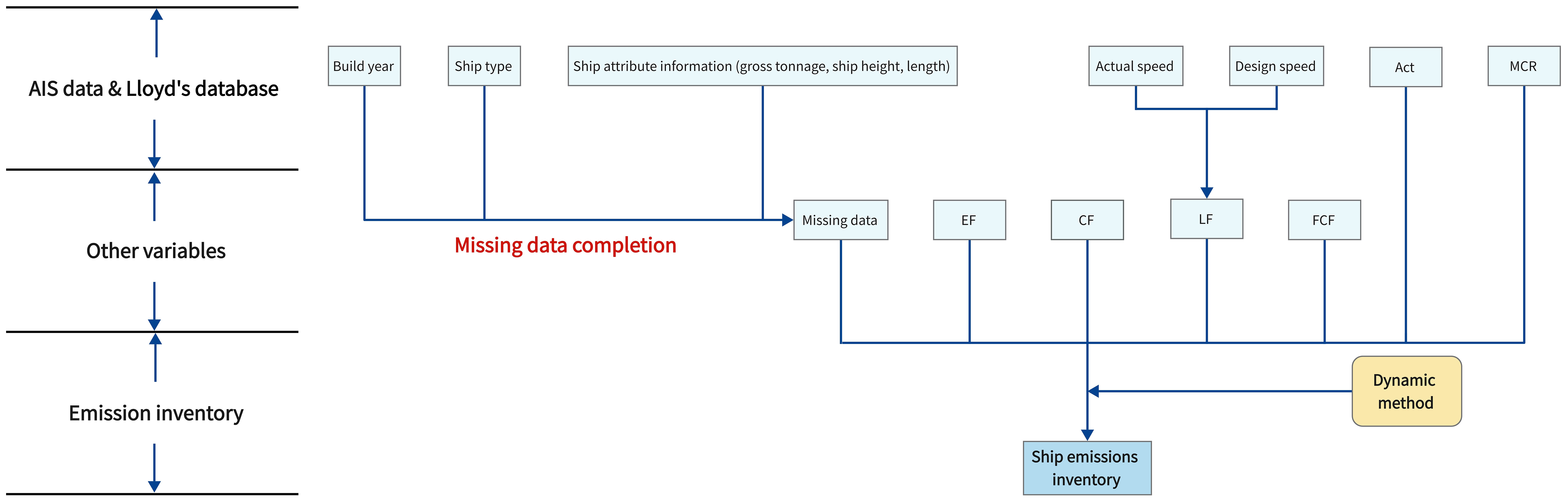
Figure 3 Flowchart of Ship Emission Inventory Calculation.
The ship power method requires determining the engine power of ship engines—including MEs, AEs, and boilers—under different sailing conditions. Emission calculations are then performed based on different pollutant emission factors, correction coefficients for these factors, and the operating time under corresponding conditions. Air pollutant emissions from non-road ships primarily arise from ship engines, comprising the ME, AE, and boiler. These engines have distinct functions: the main engine provides propulsive power for the ship and operates during cruising, low speed sailing, and maneuvering stages; the auxiliary engine supplies electrical power for lighting, air conditioning, and refrigeration; the boiler, typically active during low main engine load states, provides hot water or steam propulsion (Vehicle, 2016). In this study, emissions from these three engine types are considered, while emissions from other sources, being minimal, are ignored (Chen et al., 2017).
The navigational states of ships are classified into five categories: cruising, low speed sailing, harbor maneuvering, anchoring, and berthing. The determination of these states is based on the ship’s speed and ME loading as follows:
1) Cruising: Ship’s navigation from the port’s boundary to breakwater or deceleration zone. Speed and ME loading greater than or equal to 65%.
2) Low speed sailing: Navigation within the deceleration zone. Speed and ME loading between 20% and 65%.
3) Harbor maneuvering: Navigation from the breakwater to the pier within a port (Vehicle, 2016). Speed greater than or equal to 3 knots and main engine loading less than 20%.
4) Anchoring: Ship’s states when anchored. Speed between 1 and 3 knots.
5) Berthing: Ship’s states when docked. Speed less than 1 knot.
The formula for calculating ship engine emissions is provided by Starcrest Consulting Group and LLC (2009) as follows:
where E represents the pollutant emissions from the ship (in tons); W is the work done by the ship’s engine (in kW-h); EF is the pollutant emission factor (in g/(kW-h)); FCF is the fuel correction factor (dimensionless); and CF is the emission correction factor (dimensionless).
The formula for the work done by the ship’s engine is:
where MCR is the rated engine power (in kW), LF is the ship’s engine load factor (dimensionless), and Act is the working time (in h).
This research employs the TFT model, as delineated by Lim et al. (2021), to forecast future GHG emissions from ships. Utilizing the previously derived GHG emission inventory of Tianjin Port, essential characteristics such as time, location, and emission attributes are extracted and organized into time-series data, which then serves as input for the time-series prediction model. Notably, the prediction model adopts the TFT based on the attention mechanism, as proposed by Lim et al. (2021). For benchmarking, both RNN and long short-term memory network (LSTM) models are employed, and the TFT model’s performance is assessed using metrics like root mean square error (RMSE) and mean absolute error (MAE).
The architecture of the TFT model encompasses several modules, including a variable selection network, static covariate encoder, gating mechanism, seq2seq layer, time-based attention mechanism processing, and prediction intervals.
Grounded on the high-resolution GHG emission inventory of Tianjin Port, both static and time-variable factors related to the forecast objective are extracted for model training. Generally, multiple variables correlate with the forecast goal, yet their inter-relationships and respective weights often remain elusive. The TFT model, through its variable selection network, discerns these relationships, enabling the selection of variable weights and effectively filtering out redundant noise inputs. Simultaneously, the static covariate encoder employs a gated residual network (GRN) to embed the static feature set within the architecture.
Given the complex interactions between inputs and the target, alongside the varying degrees of nonlinear transformations required, the TFT model leverages a GRN to ensure adaptability across a broad spectrum of datasets and scenarios. On the temporal processing front, the model utilizes a seq2seq layer for local adjustments, and multi-head attention blocks to capture long-term dependencies. A distinct feature of the TFT model is its capability to generate prediction intervals based on point estimates, achieved by forecasting distinct percentiles at every temporal step, outlining a probable range of target values for each prediction interval.
This comprehensive approach to forecasting, embedded within the TFT model, aids in projecting future GHG emissions from ships, providing a robust framework for understanding and mitigating the environmental ramifications of maritime activities within Tianjin Port.
Within the TFT, the seq2seq mechanism is used to discern local dependencies present in time series, while the self-attention mechanism is employed to grasp long-term dependencies:
where , , , A() is a normalization function, commonly utilized in scaled dot-production attention:
The structure of multi-head attention is visually represented in Figure 4. Multi-head attention seeks to enhance the learning capacity inherent in the standard attention mechanism. This is accomplished by designating different heads to operate in different representation subspaces:
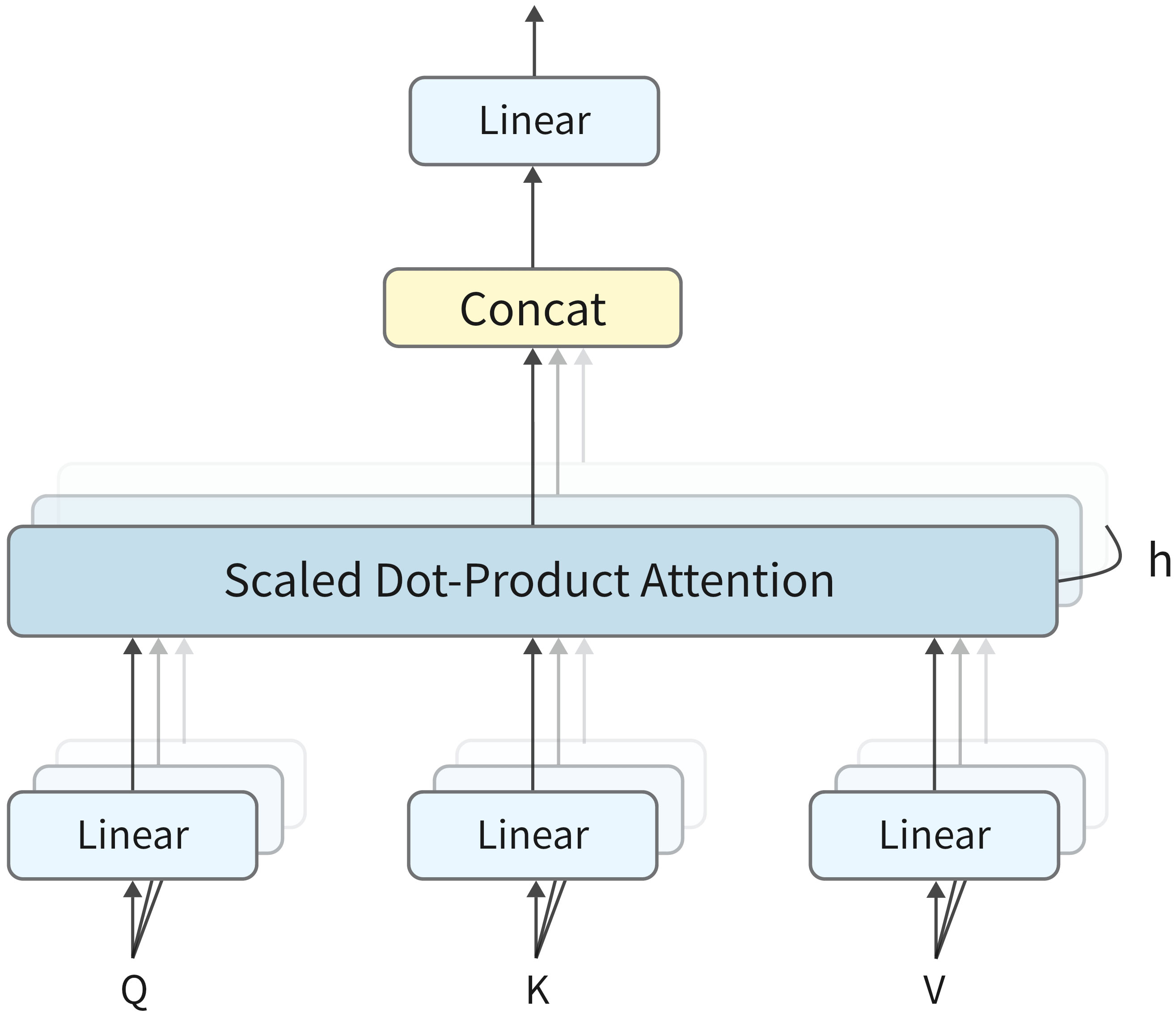
Figure 4 Schematic of the Multi-head Attention Mechanism.
where WV ∈ ℝdmodel×dV represents a weight matrix for values shared across all headers, while WH ∈ ℝdattn×dattn facilitates the final linear mapping.
Each “head” within this multi-head architecture has the capacity to learn distinct temporal patterns. Moreover, they can concurrently concentrate on the attributes of a shared set of input features. Conceptually, this can be perceived as Equation (14) where attention weights form the foundational combination matrix Ã(Q, K).
For the training and optimization of the TFT model, it was evaluated by simultaneously minimizing the quantile losses summed across all quantile outputs:
where Ω denotes the domain containing the training data consisting of M samples, W represents the TFT model’s weights, Q is the set of output quantiles (with Q = {0.1, 0.5, 0.9} utilized in our experiment, and (.)+ = max (0,.).
This study benchmarks the TFT model against RNN and LSTM for predicting GHG emissions from vessels in Tianjin Port.
A RNN is a type of neural network that does not impose constraints on the lengths of its inputs and outputs, and comprises a hidden state ht and an optional output ot at each time step t. Here, ht represents the hidden state at time t, encapsulating the information produced from all preceding time steps, while ot corresponds to the output at time t.
The function f () can range from being a basic element-wise sigmoid function to more intricate units such as LSTM. The RNN’s structure is visually represented in Figure 5.
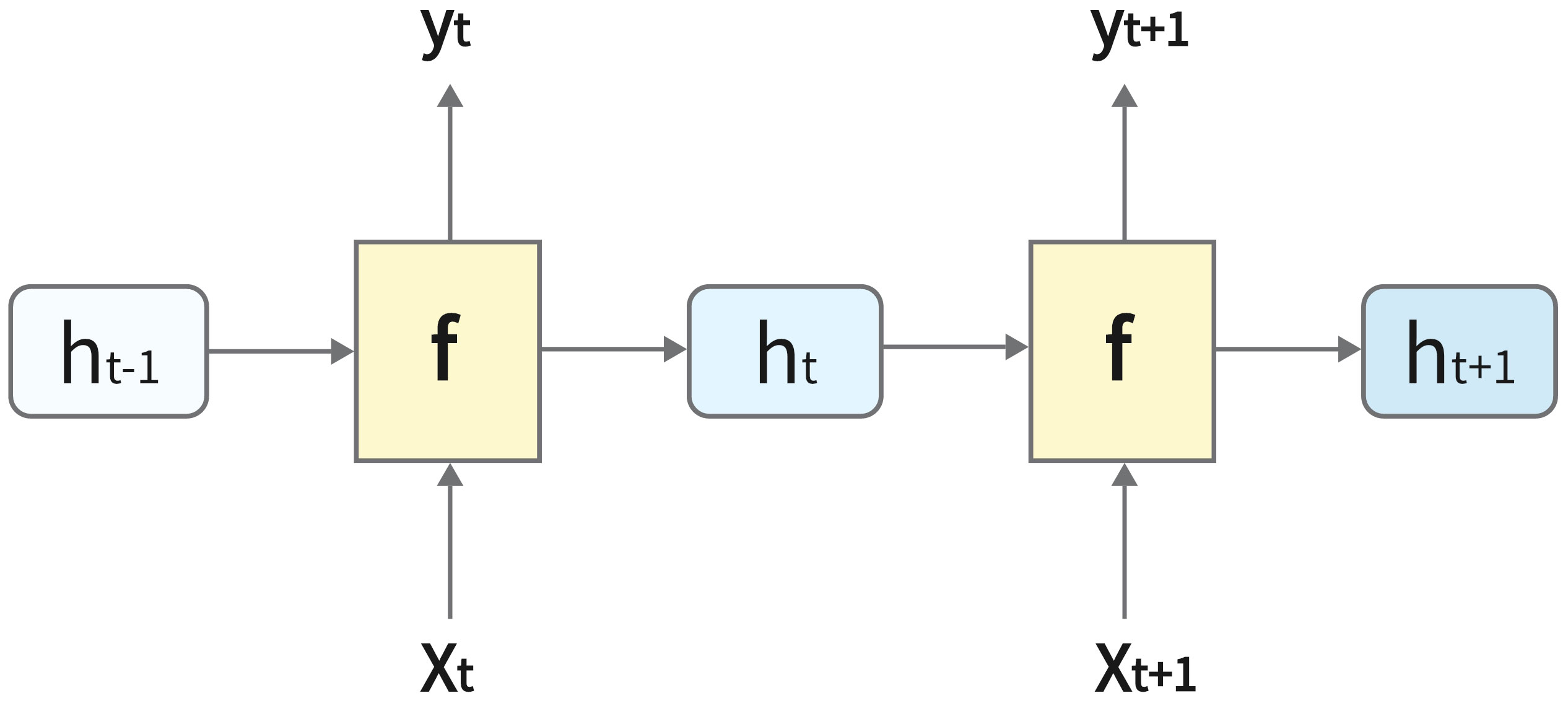
Figure 5 Schematic of the RNN Structure.
The RNN maintains consistent parameters U, V, and W across all time steps, implying that it executes the identical task at each step, albeit with varying inputs. This consistency in parameters reduces the total number of parameters to be learned, thereby enhancing computational efficiency. While outputs are generated at every time step, they may not always be requisite, depending on the specific nature of certain tasks.
The LSTM network, an extension of the conventional RNN, incorporates three distinct gates to alleviate the short-term memory issue inherent in RNNs, thereby enabling the effective utilization of long-term temporal information. By building upon the RNN structure, the LSTM introduces a forget gate layer, an input gate layer, and an output gate layer. These gates serve as logic control units that meticulously manage the flow of information and the state of memory cells in the network. Through this refined architecture, the LSTM facilitates precise control over the information flow and memory cell state, significantly enhancing the network’s capacity to capture and utilize long-term dependencies in the data. The LSTM’s structure is visually represented in Figure 6.

Figure 6 Structure of the LSTM Network.
In contrast to the RNN which possesses a singular hidden state, the LSTM network operates with two distinct states: a cell state denoted as ct and a hidden state denoted as ht. The LSTM modulates the state transmissions through the gate mechanism, selectively retaining or discarding information, which solves the long-term dependency problem well.
In this study, the accuracy of the forecasting model is assessed using RMSE and MAE as evaluation metrics. RMSE quantifies the magnitude of prediction error, representing the deviation between actual values and predicted values. It captures the spread of the actual values around the predicted regression line, with its value ranging from [0, +∞]. A larger RMSE value denotes a largerprediction error. The formula for RMSE is given as:
MAE, on the other hand, provides a linear error assessment, its value also ranging from [0, +∞]. A larger MAE value indicates a higher error. The formula for MAE is given as:
Both RMSE and MAE are commonly utilized metrics in evaluating the accuracy of models in regression problems. Lower values of these metrics signify better model performance, indicating a closer alignment of predicted values to the actual values.
In this investigation, we utilized the TFT model equipped with attention mechanisms as delineated by Lim et al. (2021) to forecast the multi-temporal and multi-spatial attributes of GHG emissions from ships in Tianjin Port. Utilizing the past 30 days’ emission data, we projected the spatiotemporal characteristics of GHG emissions for a subsequent day.
The GHG emission inventory of Tianjin Port, encompassing channels, anchorages, and berths, serves as the input data. This dataset encapsulates GHG emission information from 7 channels, 8 anchorages, and 205 berths within Tianjin harbor throughout 2018, recorded on a daily timestep. It encompasses both time-varying and static data pertinent to the prediction target. A total of 240,901 time-series data points were assembled and partitioned into training, validation, and testing sets at a ratio of 6:2:2. The training set facilitates feature learning, network parameter adjustments, and model fitting. The validation set aids in model hyper-parameter tuning and preliminary performance evaluation, while the test set evaluates the model’s generalization capability. A total of 240 iterations were conducted to ascertain optimal hyperparameters, each with an epoch count of 100. Hyperparameter optimization was carried out via random search, with the exhaustive search range of hyperparameters as follows:
• Hidden layer size: 10, 20, 40, 80, 160, 240, and 320
• Dropout rate: 0.1, 0.2, 0.3, 0.4, 0.5, 0.7, and 0.9
• Minibatch size: 64, 128, and 256
• Learning rate: 0.0001, 0.001, and 0.01
• Max gradient norm: 0.01, 1.0, and 100.0
• Num heads: 1, 4
The joint minimization of the quantile loss as described in Eqs. (7) and (8) is employed for model training and hyperparameter optimization. Experimental findings reveal that a hyperparameter configuration of hidden layer size = 20, dropout rate = 0.2, minibatch size = 256, learning rate = 0.0001, max gradient norm = 1, and num heads = 4 yields optimal predictions with a loss value approximating 0.15.
Figure 7 illustrates the fold change comparison between predicted and actual emission values in the emission inventory under Q = 0.5 and Q = 0.9 quartiles, exemplified using N2O emissions.
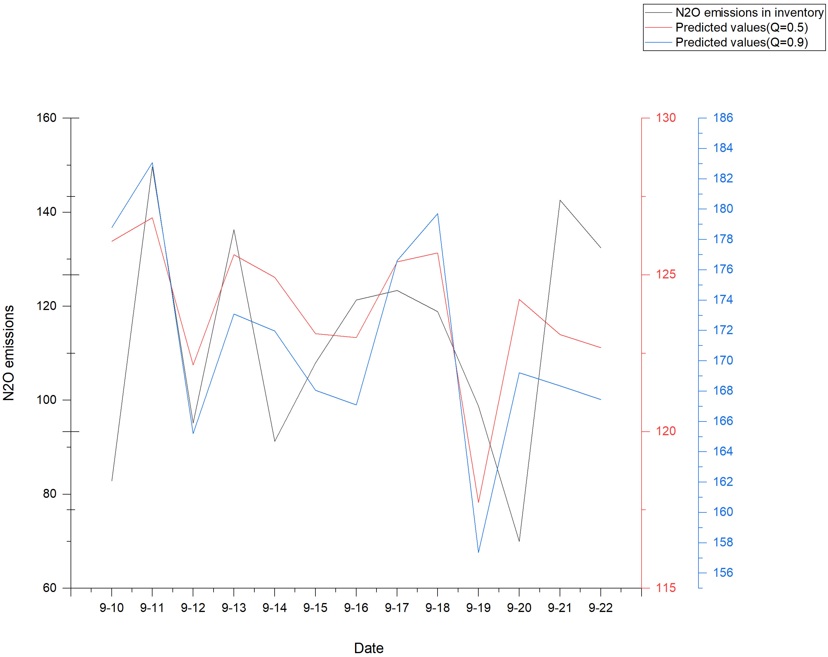
Figure 7 Prediction performance.
Table 1 presents the RMSE and MAE values of the predicted emissions for the TFT, RNN, and LSTM models, using CO2 emissions as an instance. The table illustrates that the TFT model, whether under Q = 0.5 or Q = 0.9, outperforms the traditional RNN and LSTM models.
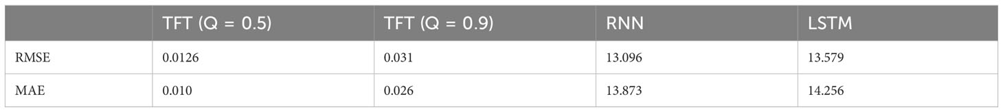
Table 1 Comparative performance of prediction models.
The initiative to incorporate the maritime industry into the EU ETS unveils numerous prospects and hurdles. It is necessary to accurately grasp the GHG emission patterns of ships, and foster the emission reduction and green transformation of the maritime sector from varying perspectives, including government and regulatory bodies, port authorities, and shipping companies. The model employed in this study forecasts the multi-emission characteristics of GHGs, encompassing CO2, CH4, and N2O, thereby offering insights into the future emission scenarios of ships within a reasonable margin of error. The government can utilize the predicted data, comprising time, location, pollutant types, and emissions, as a reference to enact preemptive measures. Such measures may include regulatory adjustments, staff mobilization, pollutant treatment, and port operation planning and scheduling, aiming to mitigate unnecessary emissions stemming from queuing, waiting, inefficient operations, and irrational planning of port facilities.
This study characterizes the GHG emissions, comprising CO2, CH4, and N2O, generated by the MEs, AEs, and boilers of ships arriving at Tianjin Port in 2018 under varied operational conditions. By combining the geographic details of Tianjin Port, a high-resolution ship GHG emission inventory is established. Various dimensions such as the emission characteristic comparison, distinct engine emission analysis, varying sailing conditions, and different ship attributes are explored to analyze the GHG emission patterns. Additionally, measures and emission reduction proposals are discussed to ensure the maritime industry’s sustainable development amid potential future challenges and opportunities, like the EU ETS.
Exhaust emissions from ships are a significant source of air pollutants. In particular, emissions of GHGs such as CO2, CH4, and N2O pose severe threats to global climate, human health, and other species’ survival. In 2018, ships entering Tianjin Port emitted approximately 674,409.27 tons of CO2, 6.93 tons of CH4, and 40.43 tons of N2O. Figures 8 and 9 illustrate the emission share ratios of each GHG and each engine type respectively in 2018.
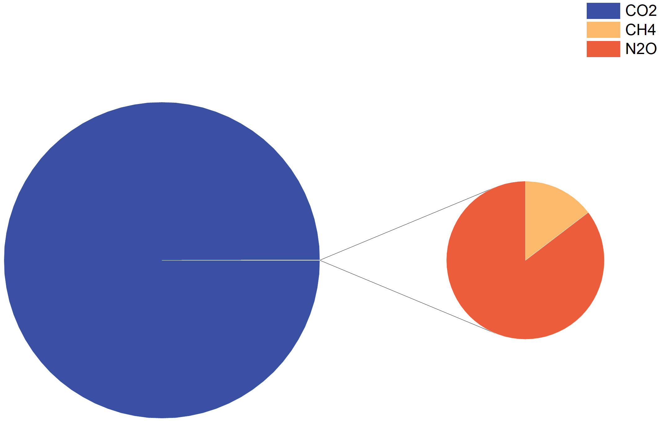
Figure 8 GHG Emission Share Ratios in Tianjin Port.
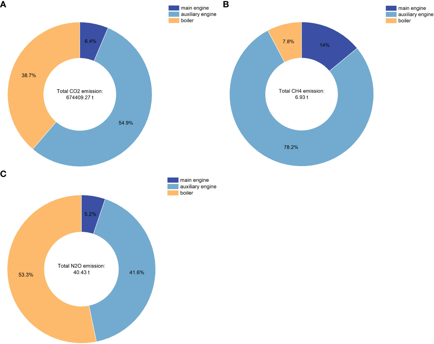
Figure 9 GHG Emission Proportions from Various Ship Engines: (A) CO2; (B) CH4; (C) N2O.
It can be observed that approximately 54.9% of CO2 emissions originate from the AEs of vessels, 38.7% from ship boilers, with a minor portion from the MEs. As for CH4 emissions, AEs stand as the predominant source, generating around 78.2% of the total, with MEs and boilers contributing approximately 14% and 7.8%, respectively. In the case of N2O emissions, about 53.3% are attributed to ship boilers, approximately 41.6% to AEs, and a minor fraction to the MEs. It reveals that AEs and boilers on ships are major contributors to the GHG emissions in Tianjin Port.
Ship engines, categorized as MEs, AEs, and boilers, serve distinct functions. MEs primarily provide propulsion power; AEs cater to lighting, air-conditioning, refrigeration, and other electrical needs; boilers are primarily for hot water or steam pumping drive (Vehicle, 2016).
Under cruising conditions, ships travel at normal speeds with boilers mostly turned off (Vehicle, 2016). As ships decelerate from normal navigation to docking, AE power increases, ME power decreases, and boilers are activated. During docking at the wharf for cargo loading and unloading using the ship’s own power system, the ME is turned off, the AE operates at a higher load, and the boiler is active. Conversely, during berthing, only the AE and boiler operate, providing the necessary electrical and thermal energy for the ship’s normal functions (Fu et al., 2012). Figure 10 illustrates the GHG emissions emitted by ships entering Tianjin Port under different operational states.
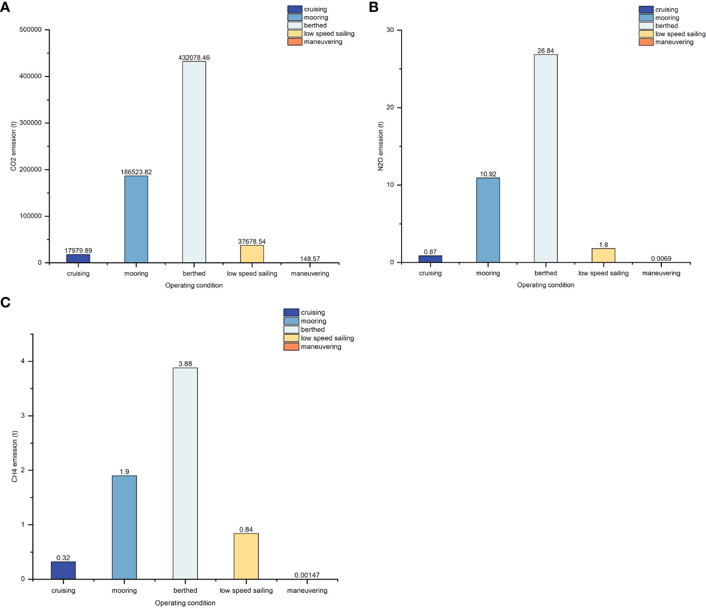
Figure 10 GHG Emissions from Ships under Different Operational States: (A) CO2; (B) N2O; (C) CH4.
The data indicate that the emissions of all three GHGs—CO2, CH4, and N2O—are significantly higher during the anchoring and berthing states, emphasizing the link between the operational states of ships within harbor waters and the resultant GHG emissions. Primarily, GHG emissions in Tianjin Port waters are generated during the phases of ship docking and cargo loading and unloading.
Studies have demonstrated that in congested waters, adopting measures such as reducing the speed of ships can effectively diminish the transit time. Additionally, utilizing dynamic planning techniques based on the planned routes and sailing information transmitted by the AIS can further optimize the transit time, enhance port operational efficiency, and elevate navigation safety (Hung et al., 2005). A notable study by Yan et al. (2018) employed a distributed parallel k-means clustering algorithm for fine path delineation to create a ship energy efficiency optimization model, considering various environmental factors. The study confirmed the efficacy of this method in reducing ship energy consumption and CO2 emissions significantly. By rational design of the port area structure and the loading/unloading processes, in alignment with the types and characteristics of ships and cargoes, and by utilizing relevant technologies for planning the entry/exit paths and cargo loading/unloading locations, ports can ensure safe and efficient operations while minimizing unnecessary pollutant emissions.
Export credit agencies (ECAs) have emerged as a key policy initiative to mitigate air pollution in ports, leveraging their technical feasibility and regulatory ease. ECAs contribute to emission reductions by enforcing strict controls on the maximum sulfur content of ship fuels. However, the stringent emission standards stipulated in export credit agreements escalate transportation costs for shipping firms. This may prompt firms to alter their routes without disrupting trade, albeit at the expense of reducing the competitiveness and attractiveness of ports (Meng et al., 2022). To balance competitiveness with emission reductions, ports are necessitated to retrofit berths and infrastructure, for instance, by installing shore power, and bear the corresponding operational and maintenance costs. Nonetheless, the high investment and operational costs associated with such retrofitting are burdensome for ports to shoulder independently (Innes and Monios, 2018). Hence, fostering collaboration among governments, ports, and shipping companies is pivotal to address these challenges effectively and promote sustainable practices in maritime operations.
Based on the data from Lloyd’s Register of Ships, it was found that ships built before the year 2000 (excluding 2000) constitute approximately 17.23% of the total number of vessels entering Tianjin Port. Notably, a higher number of aged dry bulk carriers are present among this cohort. It is recommended that the government melds subsidies with stringent regulations, where subsidies would motivate the replacement of outdated ships with newer models, and strict regulations on older ships would help prevent emissions from surpassing the stipulated standards. Additionally, the GHG emission characteristics vary among different types of ships. Figure 11 illustrates the emissions and emission share ratio of each type of ship in Tianjin Port for each month of 2018.
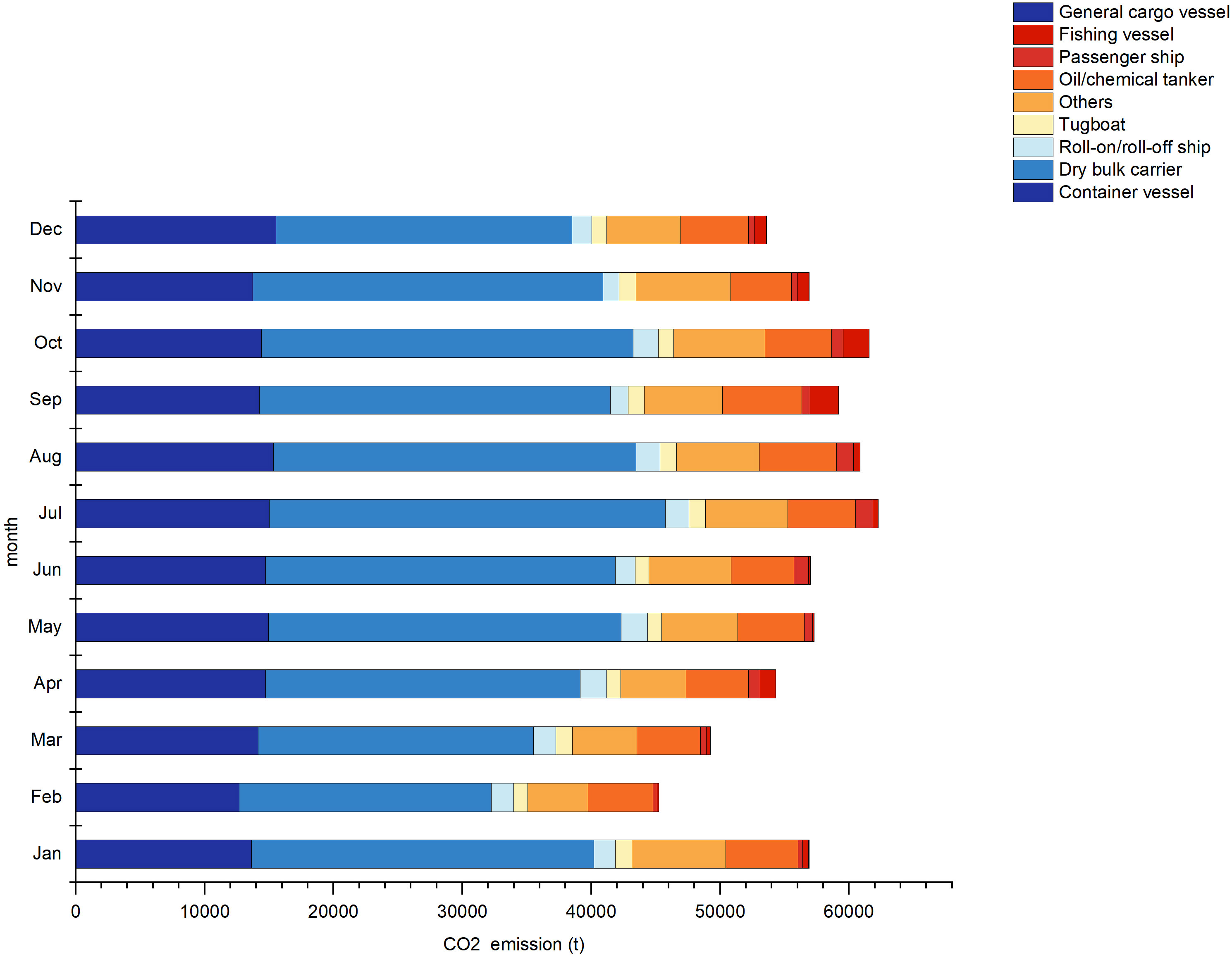
Figure 11 Emission Rates and Emission Shares of Different Types of Ships: (A) CO2; (B) N2O; (C) CH4.
As depicted in the figure, irrespective of the type of GHG emissions, dry bulk carriers, oil and chemical tankers, and container ships contribute a substantial share, with dry bulk carriers emitting the most. Dry bulk carriers account for 46.19%, 42.46%, and 47.88% of the total emissions of CO2, CH4, and N2O, respectively. Despite comprising only 9.01% of the total number of ships entering Tianjin Port, container ships account for 25.67%, 27.85%, and 25.06% of the total emissions of CO2, CH4, and N2O, respectively. The higher speeds, larger load capacities, and significantly greater engine power of container ships result in higher emissions per ship compared to other ship types, a characteristic mirrored by ro-ro ships. Though the emissions from dry bulk carriers are comparable to other ships, their sheer number, making up about 41.5% of the total ships entering Tianjin Port, leads to the highest amount of GHG emissions.
Shipping companies are primary pollution sources in inland navigation, emitting copious amounts of oily wastewater and harmful gases during voyages and port operations, thereby adversely affecting the surrounding atmosphere and waters. However, they also play a crucial role in protecting the inland river environment. By adopting clean energy technologies like shore power and liquefied natural gas, pollutant emissions can be significantly reduced (Xu et al., 2021). Recent years have witnessed the emergence of several green port transformation technologies including electric ships, clean energy, shore power, and ship exhaust treatment technologies. Yet, there is sufficient scope for advancements in technology, policy, market, and management to further mitigate environmental impacts (Wang et al., 2022). The additional costs associated with clean energy technologies can dampen the enthusiasm of shipping enterprises to engage in inland waterway environmental management. From a cost-benefit perspective, the direct costs and potential environmental benefits for local governments to monitor and control ship pollution influence their motivation, while the decision of shipping companies to adopt clean energy is closely tied to government penalties and subsidies. Eliminating the environmental impacts of ship pollution often entails higher governance costs compared to proactive regulation (Xu et al., 2021). It is imperative for local governments to increase regulatory guidance, engage other stakeholders in the governance system to actively participate in pollution control, and deploy incentives and disincentives such as carbon pricing, fuel taxes, and subsidies for clean energy projects to monitor relevant polluters (Frederiksen et al., 2021).
In this discourse, shore side electricity (SSE) pertains to the stoppage of a ship’s AE operations and its connection to onshore electricity. Ships utilizing SSE can effectively eliminate emissions from their auxiliary engines while at port berths (Karslen et al., 2019). The US Environmental Protection Agency asserts that SSE can reduce up to 98% of CO2 and other pollutants emitted by ships at berth (EPA, 2017). SSE is deemed a critical technology warranting extensive promotion (Kumar et al., 2019; Poulsen and Sampson, 2020). A qualitative study on the key stakeholders in the adoption of SSE technology recommended the introduction of this technology in ports (Meng et al., 2022).
Nevertheless, the diffusion of this technology is hindered by high construction costs and the lack of positive financial outcomes for port operators and ship owners (Dai et al., 2019; Chen et al., 2022; Ye et al., 2022). The substantial initial investments required for retrofitting port infrastructure and ship equipment pose a barrier to SSE adoption (Winkel et al., 2016). To address this issue, government regulations and port incentives are crucial. Initially, the government could subsidize a portion of the SSE equipment installation costs in ports and ships (Dai et al., 2020), as robust policies and subsidies can significantly boost the installation rate of SSE at berths. However, the high maintenance costs of SSE equipment, coupled with minimal government subsidies for SSE operations and high installation costs for ship owners, render the equipment subsidy less appealing, leading to a lack of motivation among ports and ships to adopt SSE (Yin et al., 2020). As dynamic stakeholders, ports and ships will respond according to the subsidy structure. It is a government priority to motivate ports and ships to utilize SSE.
Given the subsidy limit, the government should optimize the SSE subsidy structure for ports and ships (Wu and Wang, 2020; Wang et al., 2021; Xu and Di, 2021), elevate the subsidy on the sales price of electricity in ports, ascertain the subsidy ratio between equipment installation and operation (Wang et al., 2022), fully leverage national financial support, and enhance the relevant penalty mechanism and regulatory framework. With a guarantee of revenue, in order to obtain government subsidies rather than fines, ports may be inclined to offer certain subsidies for the emission reduction costs of shipping enterprises to encourage SSE usage (Meng et al., 2022). Concurrently, the government could take cues from the EU and devise policies to hike the tax on bunker fuels and include berthing fuel emissions in the EU ETS (Stolz et al., 2021) to foster the adoption of green transition technologies like SSE.
In the current age of environmental awareness and green transition, there is an evident increase in the release of pollution conventions and emission reduction policies. A notable example is the EU’s decision to integrate the shipping industry into the ETS. Commencing in 2026, this policy will mandate entities such as shipowners, management entities, and charterers to be financially accountable for the GHGs their vessels emit during voyages to, within, and departing from EU ports. While introducing growth prospects for new sectors like clean energy, these policies undoubtedly challenge the global shipping industry. It becomes incumbent on shipping firms worldwide to collaborate with local governments, port officials, exporters, and other key stakeholders to diligently monitor emissions and devise strategies to navigate this evolving landscape before the onslaught of more stringent international regulations.
Recognizing these changing dynamics, our research combines big data processing techniques, the dynamic method of ships, and the TFT time-series prediction model equipped with the attention mechanism. The objective is to craft a high-resolution spatiotemporal emission inventory estimation and prediction model for ship-based GHGs, tailored to manage incomplete AIS datasets. The computation part of this research offers an intricate breakdown of GHG emission trends, examining aspects such as ship type, emission-causing engine type, operational state of the ship, its construction year, and the specifics of emission time and location. Impressively, our prediction part showcases superior outcomes when compared with conventional RNN and LSTM models.
Tianjin Port, a prominent international maritime hub, stands at the crossroads of significant opportunities and challenges in its journey towards sustainable transformation. Utilizing the sea region of Tianjin Port as our primary case study, this research leverages 2018 AIS data, ship Lloyd’s records, and geographical data to initiate its emission predictions and calculations. Notably, under optimal parameter configurations, the loss is recorded at an impressive 0.15. It is worth highlighting that our emission prediction model is versatile, allowing application across diverse marine regions and temporal frames, contingent on the availability of requisite ship AIS data, Lloyd’s records, and geographic details.
This work elucidates the emission laws of GHGs from ships in the port through computation and projection of GHG emissions, thereby foreseeing the emission characteristics of ships’ GHG emissions over future time spans. This contributes to understanding the maritime transport sector’s emission characteristics, providing data and theoretical support for various stakeholders to navigate the challenges posed by the maritime industry’s inclusion in the EU ETS.
Beyond the EU ETS incorporation, the low-carbon development and green transformation of the shipping industry echo a broader global trend. As more emission reduction policies emerge, understanding how to navigate the development opportunities within the sustainable development paradigm, and addressing the imminent challenges become imperative.
For government bodies, maintaining rigorous oversight of port and shipping emissions is crucial. It necessitates the formulation of a robust policy framework to enhance carbon emissions monitoring, reporting, and verification systems, thereby building a reliable carbon emissions database. This approach seeks to address the prevailing enforcement challenges and policy imperfections in China, as highlighted by Woo et al. (2018). Additionally, the implementation of relevant subsidies alongside a reward and penalty system could foster the inception and research of cutting-edge technologies, thus boosting China’s ship energy utilization efficiency.
Port operators, on their part, can refine port structures and cargo handling processes by leveraging insights from the GHG emissions patterns of ships in ports and other environmental factors. This ensures efficient operations for ships docking at ports. Furthermore, fostering active collaborations with government authorities and shipping companies to bolster green infrastructure within ports can significantly uplift their competitive standing.
Shipping companies, amid these transitions, should meticulously evaluate their profitability strategies to strike a harmonious balance between profits and carbon emissions as outlined by Lin et al. (2017). Given the inevitable green transformation of the maritime sector and the potential surge in GHG emission costs due to tighter regulatory frameworks, maritime companies are encouraged to proactively and progressively explore avenues for low-carbon transformation and green development.
For export enterprises, the integration of the shipping industry into the EU carbon emissions framework heralds a blend of opportunities and challenges. These enterprises could opt to align with green and low-carbon shipping entities, driving the green transformation of the shipping industry from the supply chain’s end, and leveraging their influence to steer the supply chain towards sustainable development. Concurrently, staying informed with carbon emission regulation policies, assessing the potential impacts of fluctuating shipping costs on exports, optimizing global production layouts, and ensuring a semblance of profitability during the transitional phase are prudent measures, as suggested by the International Institute of Green Finance (IIGF, 2022).
The datasets generated and analysed during the current study are available from the corresponding author of QM (bWVpcWlhbmdAam11LmVkdS5jbg==) on reasonable request.
WX: Conceptualization, Data curation, Formal Analysis, Investigation, Methodology, Software, Validation, Visualization, Writing – original draft, Writing – review & editing. YL: Funding acquisition, Project administration, Supervision, Validation, Writing – review & editing. YY: Validation, Writing – review & editing. PW: Resources, Supervision, Writing – review & editing. ZW: Data curation, Software, Writing – review & editing. ZL: Software, Writing – review & editing. QM: Project administration, Resources, Supervision, Writing – review & editing. YS: Investigation, Writing – review & editing.
The author(s) declare financial support was received for the research, authorship, and/or publication of this article. This work was supported by the National Natural Science Foundation of China: [Grant Number 71804059]; the Natural Science Foundation of Fujian Province: [Grant Number 2021J01821]; Shanghai Science and Technology Committee: [Grant Number 18DZ1206300]; the National Key Research and Development Program of China: [Grant Number 2018YFC1407400].
Thanks to everyone involved in the study.
The authors declare that the research was conducted in the absence of any commercial or financial relationships that could be construed as a potential conflict of interest.
All claims expressed in this article are solely those of the authors and do not necessarily represent those of their affiliated organizations, or those of the publisher, the editors and the reviewers. Any product that may be evaluated in this article, or claim that may be made by its manufacturer, is not guaranteed or endorsed by the publisher.
The Supplementary Material for this article can be found online at: https://www.frontiersin.org/articles/10.3389/fmars.2023.1308981/full#supplementary-material
Bandemehr A., Muehling B., Corbett J., Comer B., Boyle J. (2015). U.S.-Mexico cooperation on reducing emissions from ships through a Mexican emission control area: development of the first national Mexican emission inventories for ships using the waterway network ship traffic, energy, and environmental model (STEEM). Office Int. Tribal Affairs EPA-160-R-15-001. Available at: https://www.epa.gov/international-cooperation/development-first-national-mexican-emission-inventories-ships-using (Accessed June 15, 2023).
Cariou P. (2011). Is slow steaming a sustainable means of reducing CO2 emissions from container shipping? Transportation Res. Part D 16 (3), 260–264. doi: 10.1016/j.trd.2010.12.005
Chatfield C. (1978). The holt-winters forecasting procedure. J. R. Stat. Soc. 27 (3), 264–279. doi: 10.2307/2347162
Chen D., Wang X., Li J., Zhou Y., Guo X., Zhao Y. (2017). High-spatiotemporal-resolution ship emission inventory of China based on AIS data in 2014. Sci. Total Environ. 609, 776–787. doi: 10.1016/j.scitotenv.2017.07.051
Chen D., Zhao N., Lang J., Zhou Y., Wang X., Li Y., et al. (2018). Contribution of ship emissions to the concentration of PM2.5: a comprehensive study using AIS data and WRF/Chem model in Bohai Rim Region, China. Sci. Total Environ. 610–611, 1476–1486. doi: 10.1016/j.scitotenv.2017.07.255
Chen J., Ye J., Zhuang C., Qin Q. (2022). Liner shipping alliance management: Overview and future research directions. Ocean Coast. Manage. 219, 106039. doi: 10.1016/J.OCECOAMAN.2022.106039
Chen R., Liang C., Xie F. (2013). Application of nonlinear time series forecasting methods based on support vector regression. J. Hefei Univ. Technol. (Natural Science) 36 (3), 369–374.doi: 10.3969/j.issn.1003-5060.2013.03.025
Chen Y. (2021) Research on time series Prediction Method Based on Transformer (Tianjin University). Available at: https://kns.cnki.net/KCMS/detail/detail.aspx?dbname=CMFDTEMP&filename=1023444654.nh (Accessed June 15, 2023).
Corbett J. J., Winebrake J. J., Green E. H., Kasibhatla P., Eyring V., Lauer A. (2007). Mortality from ship emissions: a global assessment. Environ. Sci. Technol. 41 (24), 8512–8518. doi: 10.1021/es071686z
Cortes C., Vapnik V. (1995). Support-vector networks. Mach. Learn. 20 (3), 273–297. doi: 10.1007/BF00994018
Dai L., Hu H., Wang Z. (2020). Is Shore Side Electricity greener? An environmental analysis and policy implications. Energy Policy(C) 137, 111144. doi: 10.1016/j.enpol.2019.111144
Dai L., Hu H., Wang Z., Shi Y., Ding W. (2019). An environmental and techno-economic analysis of shore side electricity. Transportation Res. Part D(C) 75, 223–235. doi: 10.1016/j.trd.2019.09.002
Dalsøren S. B., Eide M. S., Endresen Ø., Mjelde A., Gravir G., Isaksen I. S. A. (2009). Update on emissions and environmental impacts from the international fleet of ships: the contribution from major ship types and ports. Atmospheric Chem. Phys. 9 (161), 2171–2194. doi: 10.5194/acp-9-2171-2009
Das M., Ghosh S. K. (2014). A probabilistic approach for weather forecast using spatio-temporal inter-relationships among climate variables. 2014 9th International Conference on Industrial and Information Systems (ICIIS), Gwalior, India, 2014, 1–6. doi: 10.1109/ICIINFS.2014.7036528
Devlin J., Chang M. W., Lee K., Toutanova K. (2018). BERT: pre-training of deep bidirectional transformers for language understanding. arXiv. doi: 10.48550/arXiv.1810.04805
Endresen Ø., Sørgård E. (2003). Emission from international sea transportation and environmental impact. J. Geophysical Research: Atmospheres 108 (D17), 4560. doi: 10.1029/2002JD002898
Environmental Protection Agency (EPA). (2017) Shore power technology assessment at U.S. Ports. United states environmental protection agency. Available at: https://www.epa.gov/ports-initiative/shore-power-technology-assessment-us-ports (Accessed June 1, 2023).
Frederiksen P., Morf A., von Thenen M., Armoskaite A., Luhtala H., Schiele K. S., et al. (2021). Proposing an ecosystem services-based framework to assess sustainability impacts of maritime spatial plans (MSP-SA). Ocean Coast. Manage. 208, 105577. doi: 10.1016/j.ocecoaman.2021.105577
Fu Q., Shen Y., Zhang J. (2012). On the sip pollutant emission inventory in Shanghai port. J. Saf. Environ. 05), 57–64. doi: 10.3969/j.issn.1009-6094.2012.05.013
Gan L., Che W., Zhou M., Zhou C., Zheng Y., Zhang L., et al. (2022). Ship exhaust emission estimation and analysis using Automatic Identification System data: the west area of Shenzhen port, China, as a case study. Ocean Coast. Manage. 226, 106245. doi: 10.1016/J.OCECOAMAN.2022.106245
Goldsworthy B. (2017). Spatial and temporal allocation of ship exhaust emissions in Australian coastal waters using AIS data: analysis and treatment of data gaps. Atmospheric Environ. 163, 77–86. doi: 10.1016/j.atmosenv.2017.05.028
Goodfellow I., Bengio Y., Courville A. (2016) Deep learning (Cambridge: MIT Press) (Accessed June 26, 2023).
He L. L., Jiao Y. Q., Jia R., Liang Y. (2021). Review on the research status of air pollutant emission in port area in the development of green port. J. Chongqing Jiaotong University(Natural Science) 40 (08), 78–87. doi: 10.3969/j.issn.1674⁃0696.2021.08.11
Hulskotte J. H. J., Denier van der Gon H. A. C. (2009). Fuel consumption and associated emissions from seagoing ships at berth derived from an on-board survey. Atmospheric Environ. 44 (9), 1229–1236. doi: 10.1016/j.atmosenv.2009.10.018
Hung V. T., Hagiwara H., Tamaru H., Ohtsu K., Shoji R. (2005). Strategic collision avoidance based on planned route and navigational information transmitted by AIS. Proc. Asia Navigation Conf., 147–157. doi: ConferenceArticle/5aa3f266c095d72220bf3bb4.
IIGF. (2022). IIGF perspective | Analysis and prospects of the maritime transportation industry’s inclusion in the EU carbon emissions trading system. Available at: https://iigf.cufe.edu.cn/info/1012/6074.htm (Accessed June 1, 2023).
IMO. (2021). “Fourth greenhouse gas study 2020,” in International maritime organization (IMO). Available at: https://www.imo.org/en/OurWork/Environment/Pages/Fourth-IMO-Greenhouse-Gas-Study-2020.aspx.
Innes A., Monios J. (2018). Identifying the unique challenges of installing cold ironing at small and medium ports – The case of Aberdeen. Transportation Res. Part D: Transport Environ. 62, 298–313. doi: 10.1016/j.trd.2018.02.004
IPCC. (2007). Climate change 2007: synthesis report. Contribution of working groups I, II and III to the fourth assessment report of the intergovernmental panel on climate change. Eds. Pachauri R. K., Reisinger A. (Geneva, Switzerland: IPCC), 104.
IPCC. (2023). Summary for policymakers. in: climate change 2023: synthesis report. A Report of the Intergovernmental Panel on Climate Change. Contribution of Working Groups I, II and III to the Sixth Assessment Report of the Intergovernmental Panel on Climate Change [Core Writing Team, Lee H, Romero J, (eds.)]. IPCC, Geneva, Switzerland, 36 pages. (in press). Available at: https://www.ipcc.ch/report/sixth-assessment-report-cycle/.
Jin K. H., Wi J. A., Lee E. J., Kang S. J., Kim S. K., Kim Y. B. (2021). TrafficBERT: Pre-trained model with large-scale data for long-range traffic flow fore- casting. Expert Syst. Appl. 186, 115738. doi: 10.1016/j.eswa.2021.115738
Johansson L., Jalkanen J. P., Kukkonen J. (2017). Global assessment of shipping emissions in 2015 on a high spatial and temporal resolution. Atmospheric Environ. 167, 403–415. doi: 10.1016/j.atmosenv.2017.08.042
Karslen R., Papachristos G., Rehmatulla N. (2019). An agent-based model of climate-energy policies to promote wind propulsion technology in shipping. Environ. Innovation Societal Transitions 31, 33–53. doi: 10.1016/j.eist.2019.01.006
Kendall M., Wold H. (1954). A study in the analysis of stationary time series. R. Stat. Soc. Ser. A (General) 117 (4), 484. doi: 10.2307/2342687
Kumar J., Kumpulainen L., Kauhaniemi K. (2019). Technical design aspects of harbour area grid for shore to ship power: state of the art and future solutions. Int. J. Electrical Power Energy Syst. 104, 840–852. doi: 10.1016/j.ijepes.2018.07.051
Lara-Benıtíez P., Carranza-Garcıaí M., Riquelme J. C. (2021). Anexperimental review on deep learning architectures for time series forecasting. Int. J. Neural Syst. 31 (03), 2130001. doi: 10.1142/S0129065721300011
Li C., Borken-Kleefeld J., Zheng J., Yuan Z., Ou J., Li Y., et al. (2018). Decadal evolution of ship emissions in China from 2004 to 2013 by using an integrated AIS-based approach and projection to 2040. AtmosphericChemistryandPhysics 18 (8), 6075–6093. doi: 10.5194/acp-18-6075-2018
Li L., Ota K., Dong M. (2017). Everything is Image: CNN-based Short-Term Electrical Load Forecasting for Smart Grid. 2017 14th International Symposium on Pervasive Systems, Algorithms and Networks & 2017 11th International Conference on Frontier of Computer Science and Technology & 2017 Third International Symposium of Creative Computing (ISPAN-FCST-ISCC), Exeter, UK. 344–351. doi: 10.1109/ISPAN-FCST-ISCC.2017.78
Li C., Yuan Z. B., Ou J. M., Fan X. L., Ye S. Q., Xiao T., et al. (2016). An AIS-based high-resolution ship emission inventory and its uncertainty in pearl river delta region, China. Sci. Total Environ. 573, 1–10. doi: 10.1016/j.scitotenv.2016.07.219
Liang H., Liu S., Du J., Hu Q., Yu X. (2023). Review of deep learning applied to time series prediction. J. Front. Comput. Sci. Technol. 17 (06), 1285–1300. doi: 10.3778/j.issn.1673-9418.2211108
Lim B., Arik S. O., Loeff N., Pfister T. (2021). Temporal fusion trans-formers for interpretable multi-horizon time series forecasting. arXiv. doi: 10.48550/arXiv.1912.09363
Lin Y., Koprinska I., Rana M. (2021). SSDNet: state space decomposition neural network for time series forecasting. arXiv [Preprint].
Lin B., Liu C., Wang H., Lin R. (2017). Modeling the railway network design problem: a novel approach to considering carbon emissions reduction. Transportation Res. Part D: Transport Environ. 56, 95–109. doi: 10.1016/j.trd.2017.07.008
Liu Z., Lu X., Feng J., Fan Q., Zhang Y., Yang X. (2017). Influence of ship emissions on urban air quality: A comprehensive study using highly time-resolved online measurements and numerical simulation in shanghai. Environ. Sci. Technol. 51 (1), 202–211. doi: 10.1021/acs.est.6b03834
Mao Y., Sun C., Xu L., Liu X., Chai B., He P. (2023). A survey of time series forecasting methods based on deep learning. Microelectronic Comput. 40 (04), 8–17. doi: 10.19304/J.ISSN1000-7180.2022.0725
Mao J., Zhang Y., Yu F., Chen J., Sun J., Wang S., et al. (2020). Simulating the impacts of ship emissions on coastal air quality: importance of a high-resolution emission inventory relative to cruise- and land-based observations. Sci. Total Environment(prepublish) 728, 138454. doi: 10.1016/j.scitotenv.2020.138454
Meng L., Wang J., Yan W., Han C. (2022). A differential game model for emission reduction decisions between ports and shipping enterprises considering environmental regulations. Ocean Coast. Manage. 225, 106221. doi: 10.1016/J.OCECOAMAN.2022.106221
Mou J. M., Zhang X. S., Yao X., Li M. X. (2019). Emission inventory of ship based on navigation data in Arctic region. J. Traffic Transportation Eng. 19 (05), 116–124. doi: 10.19818/j.cnki.1671-1637.2019.05.012
Ng S. K. W., Loh C., Lin C., Booth V., Chan J. W. M., Yip A. C. K., et al. (2013). Policy change driven by an AIS-assisted marine emission inventory in Hong Kong and the pearl river delta. Atmospheric Environ. 76, 102–112. doi: 10.1016/j.atmosenv.2012.07.070
Niu F. B. (2022). On the coordinated development of port logistics and regional economy–a case study of tianjin port. J. Heze Univ 44 (04), 18–22 + 63. doi: 10.16393/j.cnki.37-1436/z.2022.04.013
Pan J. (2015) Research on key Technology of Ship AIS Data Mining (Fujian: Xiamen University). Available at: https://xueshu.baidu.com/usercenter/paper/show?paperid=f0ade0132ce43b8f9c38fea76fbf84e2&site=xueshu_se (Accessed June 1, 2023).
Pan J., Shao Z., Jiang Q. (2010). Application of data mining technology in analysis of marine traffic characteristics. Navigation China 33 (02), 60–62+73. doi: 10.3969/j.issn.1000-4653.2010.02.014
Poulsen R. T., Sampson H. (2020). A swift turnaround? Abating shipping greenhouse gas emissions via port call optimization. Transportation Res. Part D: Transport Environ. 86, 102460. doi: 10.1016/j.trd.2020.102460
Qi X., Hou K., Liu T., Yu Z., Hu S., Ou W. (2021). From known to unknown: knowledge-guided transformer for time-series sales forecasting in Alibaba. arXiv [Preprint]. doi: 10.48550/arXiv.2109.08381
Rasmussen C. E. (2004). Gaussian processes in machine learning. Advanced Lecture Mach. Learn. 3176, 63–71. doi: 10.1007/978-3-540-28650-9_4
Schuster M., Paliwal K. K. (1997). Bidirectional recurrent neural networks. IEEE Trans. Signal Process. 45 (11), 2673–2681. doi: 10.1109/78.650093
Shao Z., Sun T., Pan J., Ji X. (2007). Development of the integrated vessel information service system based on ECDIS and AIS. Navigation China 02), 30–33. doi: 10.3969/j.issn.1000-4653.2007.02.008
Slutzky E. (1937). The summation of random causes as the source of cyclic processes. Econometrica 5 (2), 105–146. doi: 10.2307/1907241
Starcrest Consulting Group, LLC (2009) The port of Los Angeles inventory of air emissions for calendar year 2009 (The port of Los Angeles). Available at: https://kentico.portoflosangeles.org/getmedia/40531068-ad9c-4e91-9b83-6da24e49dfa1/2009_Air_Emissions_Inventory (Accessed June 1, 2023).
Stolz B., Held M., Georges G. (2021). The CO2 reduction potential of shore-side electricity in Europe. Appl. Energy 285, 116425. doi: 10.1016/j.apenergy.2020.1
Tan Z. (2020). Deep Learning Based Timing Prediction and Classification. MA thesis, South China University of Technology, Guangdong, China. doi: 10.27151/d.cnki.ghnlu.2020.000504
Trozzi C. (2010). Emission Estimate Methodology for Maritime Navigation. Techne Consulting. US EPA 19th International Emissions Inventory Conference, Rome. doi: 10.3403/bsen61993
Vaswani A., Shazeer N., Parmar N., Uszkoreit J., Jones L., Gomez A. N., et al. (2017). Attention is all you need. arXiv. doi: 10.48550/arXiv.1706.03762
Vehicle Emission Control Center Ministry of Environment Protection (2016) Air pollutant emission inventory of marine in CHINA). Available at: https://www.efChina.org/Reports-zh/report-20170918-3-zh (Accessed June 1, 2023).
Wan Z., El Makhloufi A., Chen Y., Tang J. (2018). Decarbonizing the international shipping industry: solutions and policy recommendations. Mar. pollut. Bull. 126, 428–435. doi: 10.1016/j.marpolbul.2017.11.064
Wang R. B. (2022). A new path for tianjin port to build a world-class smart port. Construction Enterprise Manage 08), 108–110.
Wang C. F., Corbett J. J., Firestone J. (2008). Improving spatial representation of global ship emissions inventories. Environ. Sci. Technol. 42 (1), 193–199. doi: 10.1021/es0700799
Wang Y., Ding W., Lei D., Hao H., Jing D. (2021). How would government subsidize the port on shore side electricity usage improvement? J. Cleaner Production 278, 123893. doi: 10.1016/j.jclepro.2020.123893
Wang Y., Guo S., Dai L., Zhang Z., Hu H. (2022). Shore side electricity subsidy policy efficiency optimization: from the game theory perspective. Ocean Coast. Manage. 228, 106324. doi: 10.1016/J.OCECOAMAN.2022.106324
Wang W. Y., Li X. Y. (2021). Research on global ship spatiotemporal big data processing and visualization. Ship Electronic Eng. 41 (8), 97–103.
Wang J. Z., Wang J. J., Zhang Z. G., Guo S. P. (2011). Forecasting stock indices with back propagation neural network. Expert Syst. Appl. 38 (11), 14346–14355. doi: 10.1016/j.eswa.2011.04.222
Wei G., Yang C. (2016). Detection of AIS data error. Navication China 39 (04), 11–14. doi: 10.3969/j.issn.1000-4653.2016.04.003
Wen Q., Zhou T., Zhang C., Chen W., Ma Z., Yan J., et al. (2022). Transformers in time series: a survey. arXiv [Preprint]. doi: 10.48550/arXiv.2202.07125
Weng J. X., Li G. R. (2019). Exploring shipping accident contributory factors using association rules. J. Transportation Saf. Secur. 11 (1), 36–57. doi: 10.1080/19439962.2017.1341440
Weng J. X., Shi K., Gan X. F., Li G. R., Huang Z. (2019). Ship emission estimation with high spatial-temporal resolution in the Yangtze river estuary using AIS data. J. Cleaner Production 248 (C), 119297–119297. doi: 10.1016/j.jclepro.2019.119297
Winkel R., Weddige U., Johnsen D., Hoen V., Papaefthimiou S. (2016). Shore Side electricity in Europe: potential and environmental benefits. Energy Policy 88 584–593, 2016. doi: 10.1016/j.enpol.2015.07.013
Woo J. K., Moon D. S., Lam J. S. L. (2018). The impact of environmental policy on ports and the associated economic opportunities. Transportation Res. Part A: Policy Pract. 110, 234–242. doi: 10.1016/j.tra.2017.09.001
Wu L., Wang S. (2020). The shore power deployment problem for maritime transportation. Transportation Res. Part E(C) 135, 101883. doi: 10.1016/j.tre.2020.101883
Wu J. H., Wu C., Liu W., Guo J. W. (2017). Automatic detection and restoration algorithm for trajectory anomalies of ship AIS. Navigation Of China 40 (01), 8–12 + 101. doi: 10.3969/j.issn.1672-9730.2021.08.024
Wu S., Xiao X., Ding Q., Zhao P., Wei Y. (2020). Adversarial sparse transformer for time series forecasting. Adv. Neural In- formation Process. Syst. 33, 17105–17115. doi: 10.5555/3495724.3497159
Wu H., Xu J., Wang J., Long M. (2021). Autoformer: decomposition transformers with auto-correlation for long-term series fore- casting. arXiv [Preprint]. doi: 10.48550/arXiv.2106.13008
Xiao X., Shao Z., Pan J., Ji X. (2015). Ship trajectory clustering model based on AIS data and its application. Navigation China 38 (02), 82–86.
Xie F. (2020). Significance of air pollutant source emission inventory to regional environmental management. Resour. Economization Environ. Prot. 1), 37. doi: 10.16317/j.cnki.12-1377/x.2020.01.030
Xu L., Di Z., Chen J. (2021). Evolutionary game of inland shipping pollution control under government co-supervision. Mar. pollut. Bull. 171, 112730. doi: 10.1016/J.MARPOLBUL.2021.112730
Yan X., Wang K., Yuan Y., Jiang X., Negenborn R. R. (2018). Energy-efficient shipping: an application of big data analysis for optimizing engine speed of inland ships considering multiple environmental factors. Ocean Eng. 169, 457–468. doi: 10.1016/j.oceaneng.2018.08.050
Ye G., Zhou J., Yin W., Feng X. (2022). Are shore power and emission control area policies always effective together for pollutant emission reduction? An analysis of their joint impacts at the post-pandemic era. Ocean Coast. Manage. 224, 106182. doi: 10.1016/J.OCECOAMAN.2022.106182
Yin M., Wang Y., Zhang Q. (2020). Policy implementation barriers and economic analysis of shore power promotion in China. Transportation Res. Part D 87, 102506. doi: 10.1016/j.trd.2020.102506
Yule G. U. (1927). On a method of investigating periodicities in disturbed series, with special reference to Wolfer’s sunspot numbers. Philosophical Transactions of the Royal Society of London. Ser. A Containing Papers Math. Phys. Character 226, 267–298. doi: 10.1098/rsta.1927.0007
Zhang G. P. (2003). Time series forecasting using a hybrid ARIMA and neural network model. Neurocomputing 50, 159–175. doi: 10.1016/S0925-2312(01)00702-0
Zhang G., Patuwo B. E., Hu M. Y. (1998). Forecasting with artificial neural networks: the state of the art. Int. J. forecasting 14 (1), 35–62. doi: 10.1016/S0169-2070(97)00044-7
Zhao X., Fang Y., Wang C. (2014). Research on the technical solution of communication coverage blind area in the automatic identification system of inland river ships. Inf. Commun. 4), 29–31.
Zhao B., Yang J., Du Y. (2015). Error detection of AIS message and Research of abnormity. 11th Annu. Conf. Commun. Soc. China 2015, 1–6.
Zhou C., Huang H., Liu Z, Ding Y, Xiao J, Shu Y (2023). Identification and analysis of ship carbon emission hotspots based on data field theory: A case study in Wuhan Port. Ocean and Coastal Management 235, 106479. doi: 10.1016/J.OCECOAMAN.2023.106479
Zhou X., Leng Y. (2021). The challenges and countermeasures of developing zero-emission shipping. J. Shanghai Ship Shipping Res. 44 (04), 63–68 + 83.
Zhou T., Ma Z., Wen Q., Wang X., Sun L., Jin R. (2022). FEDformer: frequency enhanced decomposed transformer for long-term series fore- casting. arXiv [Preprint]. doi: 10.48550/arXiv.2201.12740
Zhou H. Y., Zhang S. H., Peng J. Q., Zhang S., Li J. X., Xiong H., et al. (2020). Informer: beyond efficient transformer for long sequence time-series forecasting. arXiv [Preprint]. doi: 10.48550/arXiv.2012.07436
Keywords: greenhouse gas, emission inventory, AIS, transformer, emission prediction
Citation: Xie W, Li Y, Yang Y, Wang P, Wang Z, Li Z, Mei Q and Sun Y (2023) Maritime greenhouse gas emission estimation and forecasting through AIS data analytics: a case study of Tianjin port in the context of sustainable development. Front. Mar. Sci. 10:1308981. doi: 10.3389/fmars.2023.1308981
Received: 10 October 2023; Accepted: 09 November 2023;
Published: 01 December 2023.
Edited by:
Hans Uwe Dahms, Kaohsiung Medical University, TaiwanReviewed by:
Yen-Chiang Chang, Dalian Maritime University, ChinaCopyright © 2023 Xie, Li, Yang, Wang, Wang, Li, Mei and Sun. This is an open-access article distributed under the terms of the Creative Commons Attribution License (CC BY). The use, distribution or reproduction in other forums is permitted, provided the original author(s) and the copyright owner(s) are credited and that the original publication in this journal is cited, in accordance with accepted academic practice. No use, distribution or reproduction is permitted which does not comply with these terms.
*Correspondence: Yong Li, bGkueW9uZ0BianV0LmVkdS5jbg==; Qiang Mei, bWVpcWlhbmdAam11LmVkdS5jbg==
Disclaimer: All claims expressed in this article are solely those of the authors and do not necessarily represent those of their affiliated organizations, or those of the publisher, the editors and the reviewers. Any product that may be evaluated in this article or claim that may be made by its manufacturer is not guaranteed or endorsed by the publisher.
Research integrity at Frontiers
Learn more about the work of our research integrity team to safeguard the quality of each article we publish.