Subsurface chlorophyll maxima reduce the performance of non-photochemical quenching corrections in the Southern Ocean

Non-photochemical quenching (NPQ) within phytoplankton cells often causes the daytime suppression of chlorophyll fluorescence in the Southern Ocean. This is problematic and requires accurate correction when chlorophyll fluorescence is used as a proxy for chlorophyll-a concentration or phytoplankton abundance. In this study, we reveal that Southern Ocean subsurface chlorophyll maxima (SCMs) are the largest source of uncertainty when correcting for NPQ of chlorophyll fluorescence profiles. A detailed assessment of NPQ correction methods supports this claim by taking advantage of coincident chlorophyll fluorescence and chlorophyll concentration profiles. The best performing NPQ correction methods are conditional methods that consider the mixed layer depth (MLD), subsurface fluorescence maximum (SFM) and depth of 20% surface light. Compared to existing methods, the conditional methods proposed halve the bias in corrected chlorophyll fluorescence profiles and improve the success of replicating a SFM relative to chlorophyll concentration profiles. Of existing methods, the X12 and P18 methods, perform best overall, even when considering methods supplemented by beam attenuation or backscatter data. The widely-used S08 method, is more varied in its performance between profiles and its application introduced on average up to 2% more surface bias. Despite the significant improvement of the conditional method, it still underperformed in the presence of an SCM due to 1) changes in optical properties at the SCM and 2) large gradients of chlorophyll fluorescence across the pycnocline. Additionally, we highlight that conditional methods are best applied when uncertainty in chlorophyll fluorescence yields is within 50%. This highlights the need to better characterize the bio-optics of SCMs and chlorophyll fluorescence yields in the Southern Ocean, so that chlorophyll fluorescence data can be accurately converted to chlorophyll concentration in the absence of in situ water sampling.

1 Introduction

In situ fluorometers are plagued by the day-time suppression of surface chlorophyll fluorescence in high light environments, caused by non-photochemical quenching in phytoplankton cells [NPQ; Thomalla et al. (2018); Xing et al. (2018); Xing et al. (2012)]. To correct for this effect the maximum depth that chlorophyll fluorescence is suppressed, the NPQ depth, is estimated and chlorophyll fluorescence is extrapolated upward from this depth to the surface. Many correction methods have been suggested to restore surface chlorophyll fluorescence measurements to chlorophyll concentrations (Biermann et al. (2015); Hemsley et al. (2015); Sackmann et al. (2008); Swart et al. (2015); Thomalla et al. (2018); Xing et al. (2018); Xing et al. (2012)), yet a consensus has not yet been reached on an accurate method for widespread use.

NPQ is expected to be widely prevalent in iron-limited regions of the Southern Ocean during summer when light levels are high. The suppression of chlorophyll fluorescence by NPQ is initiated by marine phytoplankton when under extreme light stress. This response prevents the build-up of harmful reactive oxidants when nutrients are severely lacking for photosynthesis, by dissipating energy away from the photosynthetic apparatus. Iron limitation in Southern Ocean phytoplankton communities has been shown to exacerbate the magnitude of NPQ (Falkowski and Kolber (1995)). As a result, innovative proxies are emerging for iron limitation based on NPQ measurements from in situ fluorometers (Schallenberg et al. (2020); Ryan-Keogh and Thomalla (2020); Ryan-Keogh and Smith (2021); Schallenberg et al. (2022); Ryan-Keogh et al. (2023)).

It is important to assess the impact of NPQ corrections on the accuracy of chlorophyll concentration estimates, as datasets from deployments of in situ fluorometers find use in large scale studies and the validation of biogeochemical models and remote sensing products (Claustre et al. (2020); Haëntjens et al. (2017)). Current assessments of NPQ corrections compare day-time measurements to a night-time reference to assess the relative accuracy of NPQ corrections. They have found that performance of NPQ correction is variable with surface stratification and in the presence of subsurface chlorophyll maxima (SCMs) (Thomalla et al. (2018); Xing et al. (2018)). Exploring these effects further in the Southern Ocean is essential, due to its high prevalence of both NPQ and SCMs in in the high-light environment of austral summer (Baldry et al. (2020)).

This work considers NPQ correction of in situ fluorescence from ship-based rosettes and biogeochemical Argo floats, to characterize the vertical distribution of phytoplankton. We assess the performance of eight NPQ correction methods in the Southern Ocean, by comparing NPQ corrected chlorophyll fluorescence to chlorophyll concentration measurements in the biological oceanography reformatting effort (BIO-MATE), which collates data from voyages (Baldry et al. (in review)). To do this we implement a new method to optimally calibrate and correct chlorophyll fluorescence for NPQ using coincident chlorophyll concentrations to identify the NPQ depth and produce a chlorophyll-informed fluorescence profile (Figure 1). We then calculate a mean sum error (MSE), biases through depth, and the success of detecting an SCM and high surface chlorophyll (HSC) after NPQ correction, compared to the chlorophyll-informed fluorescence profile “truth” to assess the performance of other NPQ methods.

Figure 1

Figure 1 Key concepts for assessing non-photochemical quenching corrections using coincident chlorophyll concentration and chlorophyll fluorescence measurements. This figure simply explains what chlorophyll-informed fluorescence is (solid green line) and how other correction methods (dashed green line) can perform worse than optimal chlorophyll-informed fluorescence correction. The relative error provides a direct measure of the deviance of a correction method from optimal chlorophyll-informed fluorescence and removes the variable profile-specific error associated with the sampling of chlorophyll concentrations. The NPQ depth derived simply from observations (NPQdobs) is not as accurate as the NPQ depth derived using the optimal correction (NPQdopt) as it relies on the sampling resolution of chlorophyll concentration measurements. Note that this is a representative figure only and the sequence of derived NPQ depth, NPQdopt and NPQdobs with depth is variable between profiles and assessed correction methods.

We attribute the variable performance of existing NPQ correction methods to high surface chlorophyll, SCMs and Southern Ocean mixing conditions. We exploit this variability and identify an optimal method for the Southern Ocean, based on the mixed layer depth (MLD), depth of the subsurface fluorescence maxima (SFM) and a modelled 20% light threshold depth [Z(rPAR20), Kim et al. (2015)]. In doing so we extend the work of Xing et al. (2018) by linking observations of SCMs to decreased performance. From these findings we provide recommendations for the correction of NPQ for chlorophyll fluorescence profiles collected on ships and floats in the Southern Ocean. These recommendations may extend into the global ocean, but further validation is needed.

2 Methods

2.1 Ship dataset

To assess the performance of NPQ correction methods, coincident profiles of chlorophyll concentration and chlorophyll fluorescence from shipboard systems were used. A common shipboard system consists of an instrument package lowered to depth via a vessel winch. The instruments typically include a conductivity, temperature and depth (CTD) sensor, a sampling rosette loaded with Niskin bottles to collect water samples and optical sensors (fluorometer, transmissometer, optical backscatter).

Ship data was accessed using the BIO-MATE data product (v1.0; Baldry et al. (in review); Baldry, 2023). BIO-MATE contains open access ship data, converted to a standard format for ease of use. This study uses data collected in the Southern Ocean (< 30°S) on 61 oceanographic voyages (Supplementary Table 1; Smetacek et al., 1997a; Smetacek et al., 1997b; CSIRO, 1998; CSIRO, 1999; CSIRO, 2000; García et al., 2002a; García et al., 2002b; Werdell and Bailey, 2002; Werdell et al., 2003; Rintoul and Rosenberg, 2004; Rintoul et al., 2004; Bidigare, 2005a; Bidigare, 2005b; Bidigare, 2005c; Bidigare, 2005d; Goericke, 2005; Morison, 2005a; Morison, 2005b; Morison, 2005c; Morison, 2005d; Morrison, 2005a; Morrison, 2005b; Morrison, 2005c; Morrison, 2005d; Morrison, 2005e; Rosenberg and Ronai, 2005; Smith, 2005a; Smith, 2005b; Smith, 2005c; Smith, 2005d; Bidigare and Landry, 2007; Buesseler et al., 2007; Carbotte et al., 2007; Barber et al., 2008; Smith, 2008; Rosenberg et al., 2010; Schröder and Wisotzki, 2010; Strass, 2010; Wright, 2010; CSIRO, 2012; Anadón and Estrada, 2013a; Anadón and Estrada, 2013b; Claustre, 2013; Wright, 2013a; Wright, 2013b; Wright, 2013c; Wright, 2013d; Wright, 2013e; Bracher, 2014; Meyer and Rohardt, 2014; Peeken and Hoffmann, 2014; Peeken and Nachtigall, 2014; Picheral et al., 2014; William and Griffiths, 2014; de Villiers et al., 2015; Gregory, 2015; Katsumata, 2015; Key et al., 2015; Uchida, 2015; CSIRO, 2016; Gregory, 2016; Katsumata et al., 2016; Macdonald, 2016; Olsen et al., 2016; Strass et al., 2016; Uchida et al., 2016; Meyer et al., 2017; Rohardt and Boebel, 2017; Sloyan and Swift, 2017; Smith, 2017; Swift, 2017; Talley, 2017; Davies et al., 2018; Iannuzzi, 2018; Schofield et al., 2018; Uchida, 2018; Bestley and Rosenberg, 2019; Bracher, 2019; Rosenberg and Gorton, 2019; Rosenberg and Rintoul, 2019; Boss and Talley, 2020a; Boss and Talley, 2020b; Clementson, 2020a; Clementson, 2020b; Clementson, 2020c; Clementson, 2020d; Rosenberg, 2020; Schofield et al., 2020), where both an in situ fluorometer was deployed on a sampling rosette and chlorophyll concentration was determined by laboratory analysis of discrete water samples, either fluorometrically or with high performance liquid chromatography. 2078 profiles were selected for analysis which had at least four chlorophyll concentration measurements shallower than the ecological mixed layer depth (EMLD, Carvalho et al. (2017), one chlorophyll concentration measurement shallower than 20 m and one measurement below the EMLD. 2841 BIOMATE profiles of chlorophyl concentration from 86 oceanographic voyages had unsuitable sampling regimes for our study based on these criteria, with most profiles only sampling surface waters. In cases where chlorophyll concentration was collected using multiple methods, high-performance liquid chromatography (HPLC) was the preferred method over fluorometric determination. Whist HPLC is the most accurate method, its inaccessibility has meant that 34% of profiles from 23 voyages were obtained using more accessible fluorometric methods. Chlorophyll concentrations marked as “not detected” were set to 0 mg m^-3.

Chlorophyll fluorescence profiles were smoothed using an abstraction method similar to that used by Satellite Relay Data Loggers deployed on elephant seals to remove fine-scale variability whilst preserving the SCM (Photopoulou et al. (2015); Guinet et al. (2013); Roquet et al. (2011)). 699 chlorophyll fluorescence profiles with high variability were removed from the analysis. We define high variability as profiles that have a residual standard error (calculated between smoothed and original profiles) that is greater than 10% of the range of the smoothed profile.

Quality assurance tests were performed on the data, including visual inspection. We removed questionable chlorophyll fluorescence profiles with suspect sensor malfunction, questionable chlorophyll measurements that showed large variance with depth when compared to fluorescence, chlorophyll fluorescence profiles that didn’t sample the entire ecological mixed layer and profiles with no variance with depth. A list of the data removed in this process is in the Supplementary Material (Supplementary Dataset 1), which included 170 chlorophyll fluorescence profiles and 146 chlorophyll concentration measurements.

After post-processing and quality assurance we identified 1222 profiles to be included in analysis, with only 132 profiles that included optical backscatter and 800 profiles that included beam attenuation. Due to the low number of profiles, we provide a comparison with optical backscatter as supplement only. We used only the shallowest 500 m of profiles. Sampling locations spanned the Southern Ocean, including the Polar Frontal Zone, the continental zone of Antarctica and the sea-ice zone. An area corresponding to the Palmer Long-Term Ecological Record (PAL-LTER) was disproportionately sampled compared to other regions. Profiles were collected between 1992 and 2017 and mostly sampled during the day in austral summer (Figure 2).

Figure 2

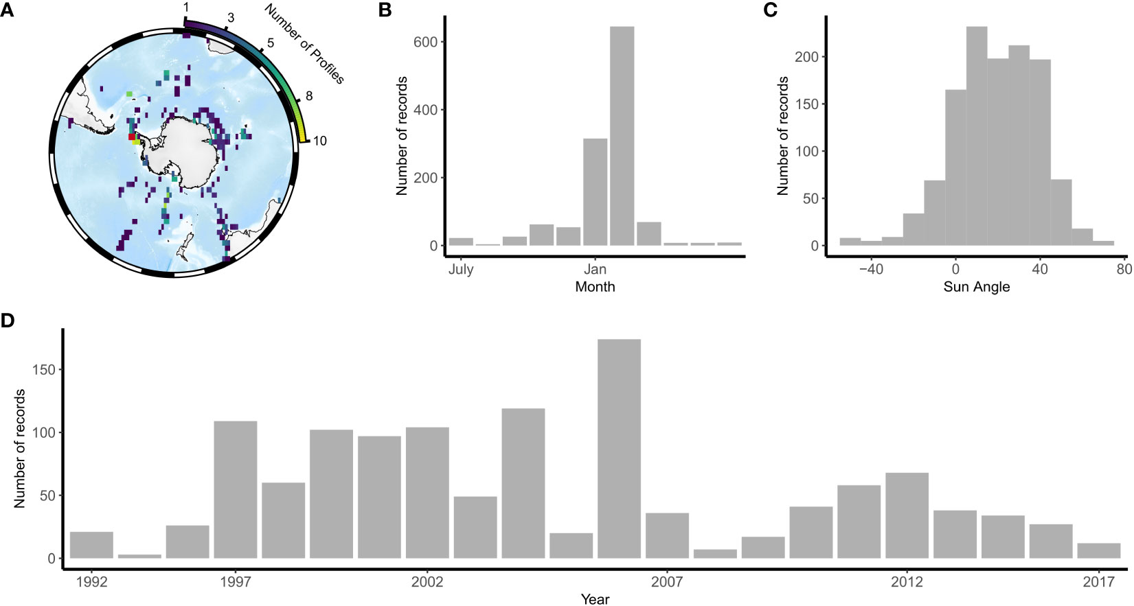
Figure 2 The spatiotemporal distribution of observations used in this study shown by (A) a spatial map showing the location and density of observations (B) frequency distributions of observations through time (C) frequency distribution of observations by month and (D) frequency distribution of observations by sun angle, where positive sun angles indicate daytime measurements. In (A) the red box shows the PALMER LTER region which has an observation density of up to 150 profiles.

2.2 Characterizing chlorophyll features

The performance of NPQ correction methods were explored over their ability to detect two common chlorophyll profile features; subsurface chlorophyll maxima (SCMs) and high surface chlorophyll (HSC). SCMs were defined as being present when the maximum chlorophyll concentration was not at the surface (< 20 m). To minimize the number of false detections due to measurement uncertainty, SCMs were defined if they met one of two criteria based on chlorophyll concentration. For surface chlorophyll concentrations < 1 mg m^-3, chlorophyll concentrations at the SCM were required to be greater than the surface by 0.2 mg m^-3. For surface chlorophyll concentrations > 1 mg m^-3, chlorophyll concentrations at the SCM had to be greater than 1.2 times the surface chlorophyll concentrations. A subsurface fluorescence maximum (SFM) was detected with the same criteria, using chlorophyll fluorescence calibrated to chlorophyll concentrations. These thresholds were chosen so that the detection of a SCM was less sensitive to measurement errors at small concentrations.

An HSC was defined if chlorophyll concentrations averaged over 10 m layers decreased from the surface to 100 m (Lavigne et al. (2015)), and surface chlorophyll concentration was greater than 0.5 mg m^-3. High surface fluorescence (HSF) was detected with the same criteria as HSC, using chlorophyll fluorescence calibrated to chlorophyll concentrations.

2.3 Characterization of mixing regimes

To understand the impact of ocean conditions on the performance of NPQ corrections, we considered different ocean conditions.

1. The mixed layer depth (MLD) was shallower than the SFM.

2. The MLD was deeper than the SFM.

3. A freshwater layer (FWL) likely due to recent ice-melt; characterized by salinity and temperature minima above the MLD.

The MLD was defined using a 0.03 kg m^-3 density increase relative 10 m.

2.4 Smoothing of data profiles

Fluorescence, backscatter, beam attenuation and density profiles were smoothed to remove fine scale variability, sensor noise and to remain comparable to the depth resolution of chlorophyll concentration measurements (Figure 3). An abstraction method of smoothing reduces a profile to piecewise linear fits (Photopoulou et al. (2015); Guinet et al. (2013)). The benefits of using an abstraction method, against more widely accepted smoothing methods, including non-linear fits (Ardyna et al. (2013); Carranza et al. (2018)) and moving mean or median windows (Cornec et al. (2021)), are that it minimizes the suppression of a thin SCM feature, is not influenced by spikes and can be applied to a wide range of profile shapes. The abstraction method was built using the segmented.lm function from the R package segmented. The method is highly adaptable, and its performance is not impacted by sampling resolution. Full code for the fit_segmented_bp function is available at github.com/KimBaldry/Ocean_code/cleaning/BSM.

Figure 3

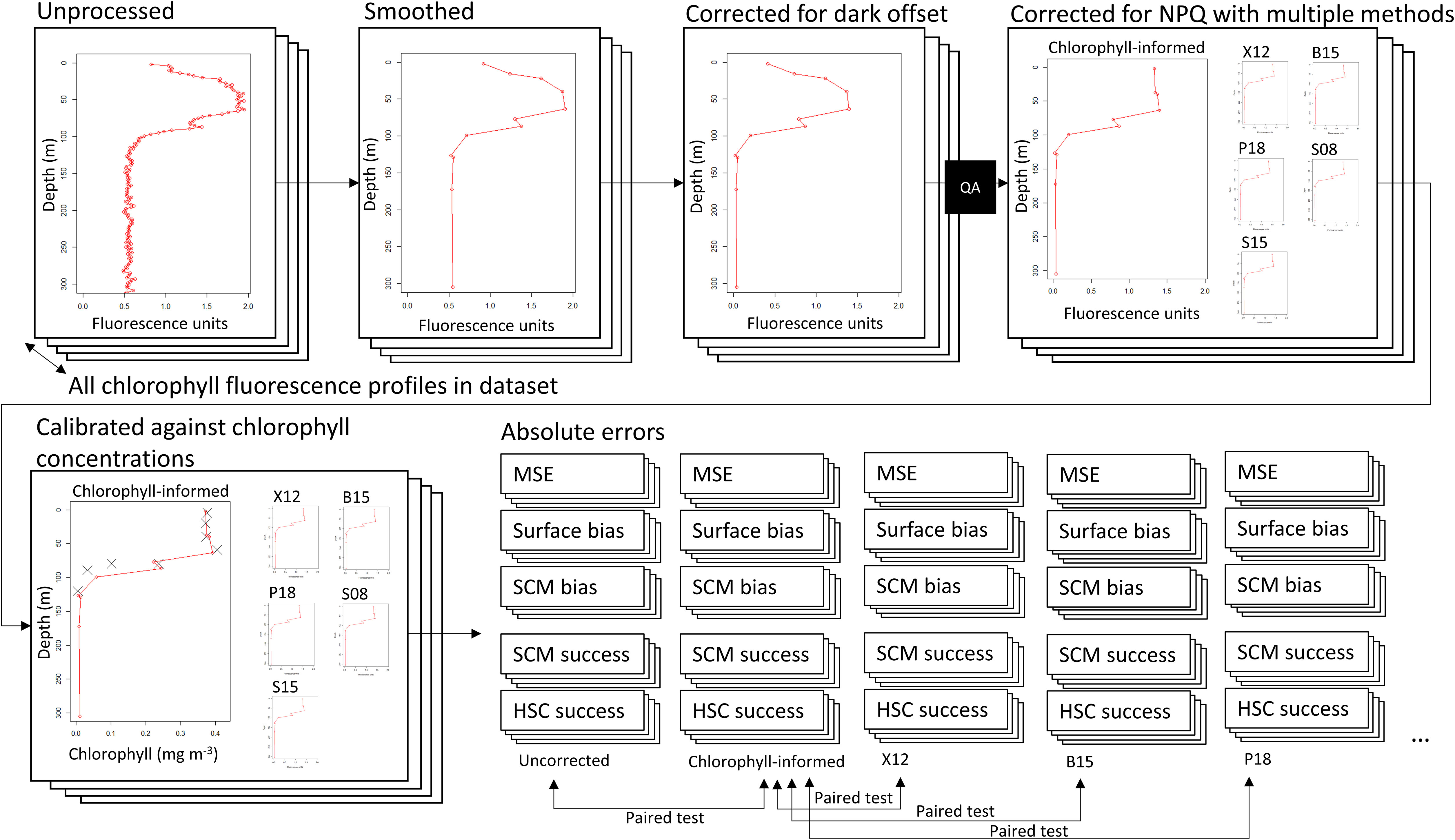
Figure 3 A diagram illustrating the data processing required to calculate comparison measured across a large set of chlorophyll fluorescence profiles. Uncorrected profile data are smoothed and corrected for a dark offset before undergoing visual quality assurance. Quality assured profiles are corrected for NPQ using the chlorophyll-informed and existing NPQ methods. Corrected profiles are then calibrated against chlorophyll concentration measurements to allow comparison measures to be calculated. Paired comparisons are then performed on chlorophyll-informed fluorescence relative to uncorrected data, and on existing NPQ correction methods compared to chlorophyll informed fluorescence.

The fit_segmented_bp function fits a piece wise linear model, optimizing the placement of several break points. It applies the segmented.lm function, and increases the number of breakpoints iteratively. When an additional break point is added, it checks that both the residual standard error and Bayesian information criterion (BIC) of the fit have decreased. The function decides on a final number of break points when five sequential break points fail this check. When the final number of break points are found, outliers outside three standard deviations of the residuals are removed by the function and the piece wise model is re-fit. This yields the final piecewise linear model that creates a smoothed profile without over-fitting.

The fit_segmented_bp function was applied to smooth density profiles as described. A two-step method was used to smooth chlorophyll fluorescence, backscatter and beam attenuation profiles, by applying the fit_segmented_bp function to a top portion of the profile (depths above the deepest depth of 80^th percentile measurement minus 75 m), and a bottom portion of the profile with little variability (up to 500 m). We found this abstraction method was able to capture SCMs well and rarely suppressed their magnitude, even when the SCM was thin (3-10 m; Supplementary Figure 1). Smoothed chlorophyll fluorescence, beam attenuation and backscatter profiles were then adjusted using a dark offset, calculated as the minimum value of a linear fit of the bottom portion of the profile. If backscatter profiles were higher than 3 m resolution, they were first despised using a 5-point running median before smoothing as recommended (Cornec et al. (2021)).

2.5 Optimally correcting NPQ using coincident chlorophyll concentrations

We developed a method to correct chlorophyll fluorescence profiles for NPQ using coincident chlorophyll concentrations (Figure 3). Coincident chlorophyll fluorescence measurements were obtained by averaging chlorophyll fluorescence over a 2 m window spanning the chlorophyll sampling depths. The 2 m window attempts to partially account for heave and the potential 1-2 m difference between the fluorometer and Niskin bottle. We then endeavored to calculate the NPQ depth, the deepest depth at which NPQ affects chlorophyll fluorescence for an optimal correction.

Paired observations of chlorophyll concentrations and chlorophyll fluorescence were used to determine NPQ depth (NPQdobs): the deepest measurement where the chlorophyll concentration to chlorophyll fluorescence ratio consecutively decreased from the surface. However, this only considers fluorescence values at depths where there are chlorophyll concentration measurements and is dependent on the depth resolution chlorophyll concentrations.

Thus, there is a need for an optimally calculated NPQ depth (NPQdopt) which we calculated from chlorophyll-informed fluorescence. To derive chlorophyll-informed fluorescence profiles a constant upward correction from an NPQdopt was performed according to X12 [CF_X12; Xing et al. (2012)] or a variable upward correction according to S08 with beam attenuation [CF_S08; Sackmann et al. (2008)]. The chlorophyll-informed fluorescence profile is used as a “truth” to assess NPQ correction methods, and may also be useful to robustly correct large datasets of ship-base chlorophyll fluorescence in an automated way.

To derive NPQdopt first a chlorophyll fluorescence calibration scalar and a NPQ depth were coincidently varied to minimize a weighted residual sum of squares between chlorophyll fluorescence and coincident chlorophyll concentrations, weighted towards the maximum chlorophyll concentration [chlorophyll/(maximum chlorophyll²)] to prevent an increase in error from deeper samples. This minimization problem was solved using the optim function in the R stats package according to Byrd et al. (1995). After this step, NPQ depth was further adjusted using the same method, only with the newly constrained calibration scalar held to its fixed value calculated in the first step. A solution to this two-step minimization problem with an assumed constant upward correction yielded CF_X12, and a separate solution with assumed variable upward correction following beam attenuation yielded CF_S08. Constraints were put in that the NPQdopt had to be shallower than the EMLD and the corrected values were always greater than or equal to the uncorrected values. In the case of constant upward correction (CF_X12), the NPQdopt had to be 5m above the SCM if one was present.

For uncorrected (but calibrated) chlorophyll fluorescence and chlorophyll-informed fluorescence we calculated the mean sum error (MSE) relative to chlorophyll concentrations and a bias at the surface and at the SCM relative to chlorophyll concentrations. Significant differences in MSE, surface bias and SCM bias between uncorrected chlorophyll fluorescence and chlorophyll-informed corrected chlorophyll fluorescence were detected using a two-sided pair-wise Wilcoxon robust test (for continuous variables) or a McNemar’s chi-squared test for symmetry (binary variables) to a 97.5% confidence level. The ability of an optimally corrected chlorophyll fluorescence profile to reproduce chlorophyll profile shape was determined as the accuracy of detecting SCMs and HSC from chlorophyll fluorescence.

2.6 Identifying NPQ

To identify significant NPQ in chlorophyll fluorescence data, we compared chlorophyll-informed fluorescence using a constant upward correction (CF_X12) to uncorrected chlorophyll fluorescence. For surface chlorophyll concentrations < 1 mg m^-3, NPQ was detected as uncorrected chlorophyll fluorescence less than chlorophyll-informed fluorescence by at least 0.1 mg m^-3. For surface chlorophyll concentrations > 1 mg m^-3, NPQ was detected as uncorrected chlorophyll fluorescence at least 10% less than chlorophyll-informed fluorescence. These thresholds were chosen so that the detection of NPQ was less sensitive to measurement errors at small concentrations.

2.7 Pre-existing NPQ correction methods

Of the eleven existing NPQ correction methods we assess six (Table 1). The remaining five methods either require day and night sampling or PAR data. Methods which require day and night sampling have already been adequately assessed (Thomalla et al. (2018)) and are not widely suitable for application to biogeochemical Argo floats and ship-based sampling. We also test variations of the X12+ and S08+ methods in the absence of radiometers, by approximating the proportion of surface PAR available at depth (rPAR) and testing various light thresholds for NPQ depth in place of MLD. We approximated rPAR by extrapolating chlorophyll fluorescence to the surface and using the methods of Kim et al. (2015) outlined in Xing et al. (2018).

Table 1

Table 1 Pre-existing NPQ corrections that have been implemented on chlorophyll fluorescence profiles, and an indication if they can be applied to the BGC-Argo dataset.

Four methods, S08, S08eu, S15 and S15eu, are only suitable when optical backscatter sensors are deployed in tandem with fluorometers, which is the case for the biogeochemical Argo network and is becoming more common on ships. Historically, ships have been equipped with beam attenuation sensors (transmissometers) rather than optical backscatter sensors, so we also test variations of S08, S08eu, S15, S15eu with beam attenuation in the place of backscatter.

Smoothed chlorophyll fluorescence profiles were corrected by a NPQ correction method and then were calibrated to coincident chlorophyll concentration measurements, similar to the process described in Section 2.5. To solve for a calibration scalar, a one-step method optimization problem was solved to minimize the weighted residual sum of squares according to Byrd et al. (1995). The entire NPQ corrected chlorophyll fluorescence profile was then calibrated with this scalar.

2.8 Assessment of NPQ correction performance

To assess the performance of NPQ methods, after calibrating and correcting profiles according to different methods, we calculated the mean sum error (MSE) relative to chlorophyll concentrations and a bias at the surface and at the SCM relative to chlorophyll concentrations and define these measurements as the absolute errors in corrected chlorophyll fluorescence (Figure 3). The absolute error derived from chlorophyll-informed fluorescence profiles (CF_X12 or CF_S08) is used as a baseline (or “truth) and subtracting it from the absolute errors calculated from applying each NPQ correction method then gives a relative error. This relative error is attributed to the application of a NPQ correction (e.g. X12) that is not the optimal chlorophyl-informed correction (i.e. CF_X12 or CF_S08) and is unaffected by difference in accuracies between sampling methods (ie. HPLC vs Fluorometry) and analysis conditions across profiles. Significant differences in absolute MSE and bias measures across methods were detected using a pair-wise Wilcoxon robust test (for continuous variables: MSE, surface bias and SCM bias) or a McNemar’s chi-squared test for symmetry (binary variables: SCM and HSC occurrences) to a 97.5% confidence level.

The effects of significant NPQ, the presence of an SCM or HSC, were analyzed by comparing absolute MSE and bias measures across effect groups (e.g. SCM vs no SCM). Significant effects were detected using a Kolmogorov–Smirnov test (continuous variables) or a Pearsons chi-squared test (binary variables) for differences in distribution between effect groups with a confidence level of 97.5%. The effect of different ocean regimes was also analyzed by comparing measures across groups, however, to detect significant differences between effect groups a Kruskal-Wallis test was used in place of the Kolmogorov–Smirnov test.

3 Results

3.1 Chlorophyll-informed fluorescence

The comparison showed CF_X12 and CF_S08 were able to calibrate chlorophyll fluorescence and correct for NPQ in 90% of chlorophyll fluorescence profiles to within a 21% and 30% MSE, respectively. Visual inspection confirmed that the chlorophyll-informed fluorescence was most ideally calibrated and corrected for NPQ, and that sampling errors in chlorophyll concentration, not inaccurate beam attenuation data, lead to 24 cases (9 HSC) where MSE was at least 25% larger in CF_S08 compared to CF_X12 (Supplementary Figure 1). To ensure that these outliers did not influence our comparison they were excluded and the statistics re-run. After their removal 90% of remaining CF_S08 profiles showed a MSE of 22% (Table 2).

Table 2

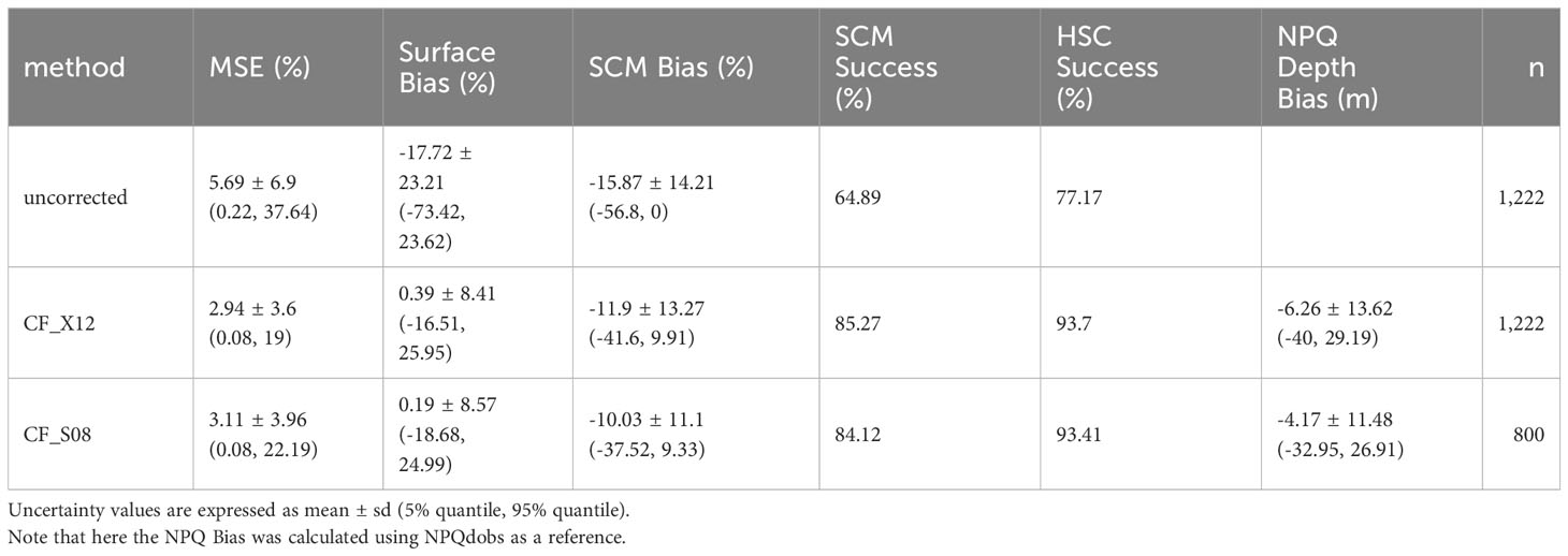
Table 2 Absolute error measures in uncorrected chlorophyll fluorescence profiles and chlorophyll-informed fluorescence profiles (CF_X12 and CF_S08), compared to chlorophyll concentration profiles.

The ability of CF_X12 and CF_S08 to reproduce chlorophyll profiles were comparable as indicated by MSE of 2.94 (± 3.6) % and 3.11 (± 3.96) %, and chlorophyll bias at the surface of 0.39 (± 8.41) % and 0.19 (± 8.57) %, respectively (Table 2). Chlorophyll bias at the SCM was -11.9 (± 13.27) % for CF_X12 and -10.03 (± 11.10) % for CF_S08. Compared to the observed measure of NPQ depth (NPQdobs) calculated by comparing chlorophyll concentrations to uncorrected fluorescence, the CF_X12 and CF_S08 methods chose significantly different NPQ depths, on average choosing a shallower depth with a mean bias of -6.26 (± 13.62) m and -4.17 (± 11.48) m respectively. This difference is expected due to differences in depth resolution but demonstrates that the optimal methods are reproducing what would be subjectively determined by an observer.

Uncorrected chlorophyll fluorescence profiles affected by NPQ displayed significantly higher MSE, significantly underestimated surface chlorophyll, and had large SCM bias. Significant differences in CF_X12 and CF_S08 were still observed in surface chlorophyll bias and MSE between quenched and unquenched profiles, and SCM chlorophyll bias using the CF_X12 method specifically. However, these significant differences were a lot smaller compared to uncorrected data, reducing surface chlorophyll bias by on average 40% and MSE by 8% in quenched data (Table 3).

Table 3

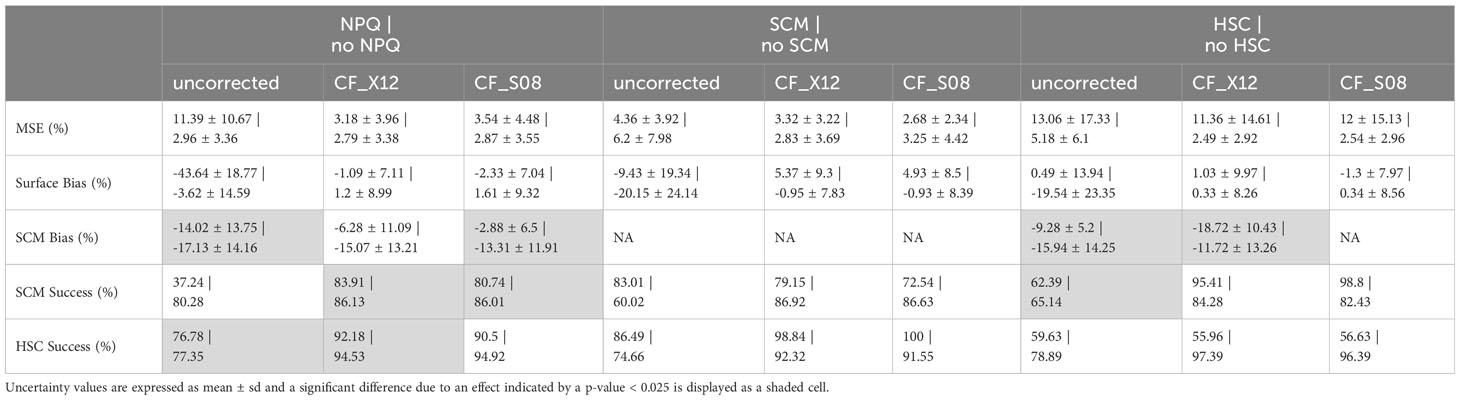
Table 3 Effects of NPQ, SCM presence and HSC presence on absolute errors in uncorrected chlorophyll fluorescence profiles and chlorophyll-informed fluorescence profiles (CF_X12 and CF_S08), compared to chlorophyll concentration profiles.

3.2 Identifying SCMs and HSCs from chlorophyll-informed fluorescence

Chlorophyll-informed fluorescence significantly increased the accuracy of detecting an SCM from chlorophyll concentrations (Table 2). The CF_X12 and CF_S08 methods had an accuracy of 85.27% and 84.12% for SCM detection compared to 64.89% in uncorrected chlorophyll fluorescence. Similarly, the chlorophyll-informed methods significantly increased the accuracy of detecting HSCs, with the CF_X12 and CF_S08 methods replicating 93.70% and 93.41% of HSCs compared to 77.17% in uncorrected data.

Chlorophyll-informed fluorescence showed some variability in performance when the presence or absence of an SCM is considered (Table 3). In the case of chlorophyll-informed fluorescence derived from only fluorescence (CF_X12), when an SCM was present a slightly higher MSE and a significant overestimation of chlorophyll at the surface was observed compared to when no SCM was present. When beam attenuation information was used (CF_S08) it displayed lower MSE, lower surface error and performed better than CF_X12 in the presence of an SCM.

When a HSC was observed chlorophyll-informed fluorescence displayed a higher MSE and more variable surface chlorophyll bias. Both the CF_X12 and CF_S08 methods were significantly better at replicating a HSC absence compared to a presence (Table 3). Upon visual inspection, we found that CF_X12 was unable to reproduce surface chlorophyll trends in 12 profiles (5.0%) with HSC, 9 of which were removed. Additionally, CF_X12 led to an overestimation of surface chlorophyll in 7 profiles (3.1%) with a strong SCM, by calculating an NPQ depth that was too deep.

3.3 Assessment of pre-existing NPQ corrections

Compared to uncorrected profiles, all NPQ correction methods removed or reduced the surface NPQ signal in chlorophyll fluorescence profiles and decreased absolute MSE (Supplementary Table 2). The B15 and S15eu methods led to a notably high absolute surface chlorophyll bias and over-correction due to calculating NPQ depths too deep. Compared to uncorrected profiles, all correction methods, both using beam attenuation and not, improved the absolute success of reproducing an SCM and HSC observed in chlorophyll measurements. All methods on average chose NPQ depths 3-14 m deeper than the observed NPQ depth.

Compared to chlorophyll-informed corrected profiles, no method was able to reproduce significantly similar relative MSE, surface chlorophyll bias, SCM chlorophyll bias or NPQdopt (Table 4). The X12, P18 and S08 methods showed a significantly similar success in detecting an SFM feature compared to chlorophyll-informed fluorescence, only in the beam attenuation comparison subset. All methods could produce statistically similar HSF success within the beam attenuation comparison subset, but not across the full fluorescence only comparison dataset. On average, all existing methods tended to calculate NPQ depths 5 – 20 m deeper than those calculated using chlorophyll informed correction methods.

The P18 method performed the best when considering relative MSE (0.47 (± 1.06) %), relative surface chlorophyll bias (1.79 (± 8.23) %) and relative SCM chlorophyll bias (-2.66 (± 4.79) %). X12 performed similarly, with a relative MSE of 0.47 (± 1.07) %, relative surface chlorophyll bias of 2.07 (± 8.12) % and relative SCM chlorophyll bias of -2.96 (± 5.12) %. The S08 method was the best of when beam attenuation was implemented, showing a similar relative MSE to P18 and a higher rate of SCM success. The B15 and S15eu corrections performed the worst across relative MSE, surface bias and SCM bias, tending to underestimate the SCM, overestimate surface chlorophyll and choose a deeper and more variable NPQ depth, leading to overcorrection compared to chlorophyll-informed NPQdopt. The S15 method also performed badly, tending to overcorrect for NPQ and lead to a high rate of destroyed SCMs (Table 4).

Table 4

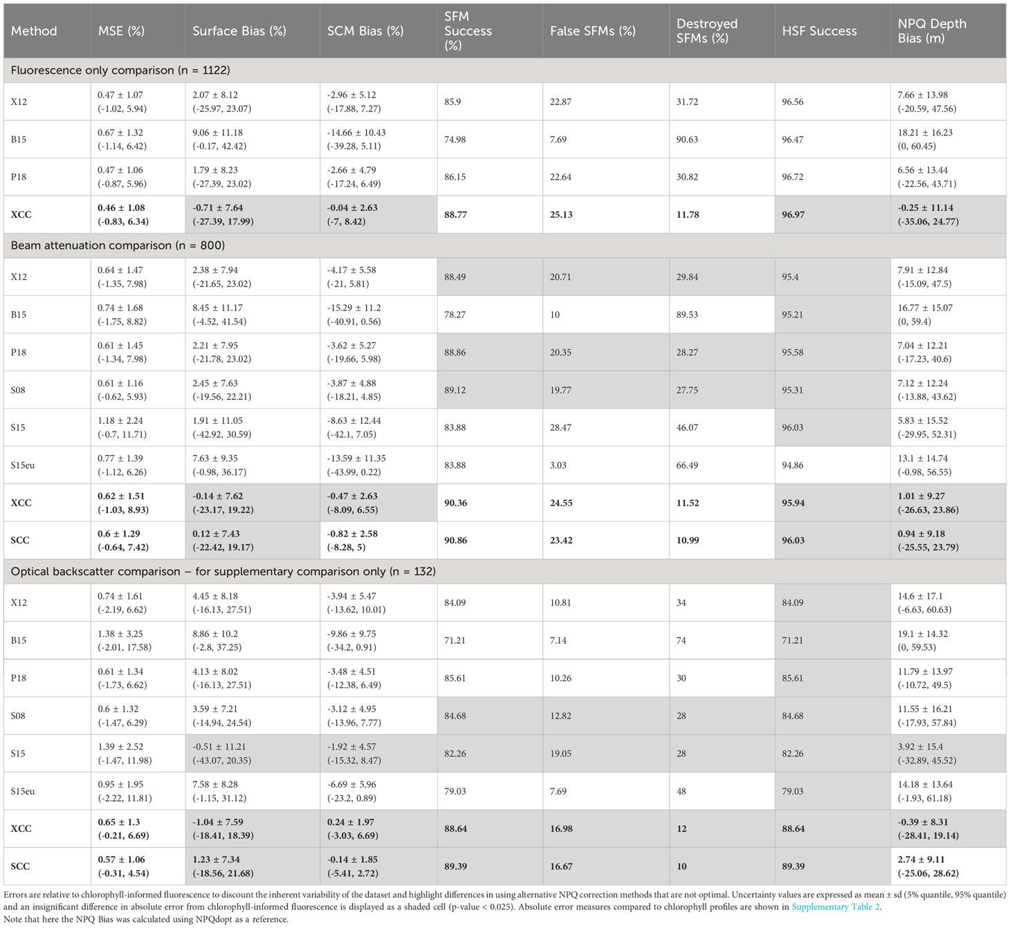
Table 4 Relative error measures in NPQ corrected chlorophyll fluorescence profiles across different NPQ correction methods, newly defined methods are bolded.

3.4 Higher MSE and underestimation of chlorophyll with significant NPQ

Overall, higher MSE is observed across all methods when significant NPQ is observed (Table 5). When significant NPQ is observed, the X12 and P18 methods displays higher MSE compared to B15 and S15eu. However, the B15 and S15 show large overestimation of surface chlorophyll and underestimation of the SCM, leading to a low SFM success rate due to a high rate of Destroyed SFMs in the presence of significant NPQ. When significant NPQ is not observed, surface chlorophyll is on average overestimated by all methods. There is little effect on the SCM bias when the effect of significant NPQ is considered.

Table 5

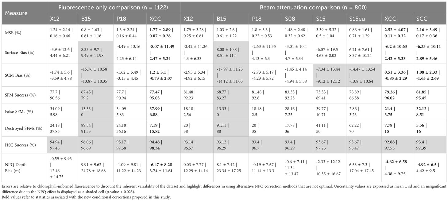
Table 5 Select relative error measures in NPQ corrected chlorophyll fluorescence profiles across different NPQ correction methods, split to show the effect of NPQ presence vs. NPQ absence (NPQ | no NPQ).

The best performing pre-existing X12, P18 and S08 methods do not correct fully for the effects of NPQ, underestimating surface chlorophyll by 4-5%. This leads to 34% of detected SFMs being false SFMs compared to chlorophyll-informed fluorescence (Table 4).

3.5 Higher MSE when an SCM is identified

258 SCMs were detected, accounting for 21.1% of chlorophyll concentration profiles. Most SCMs were observed below the MLD, however 14% of SCMs were observed above the MLD. 37% of SCMs formed above the euphotic depth, at high light levels of up to 30% surface light. 80% of SCMs formed under conditions where the MLD was shallower than the euphotic depth. When the MLD is shallower than the euphotic depth 99% of SCMs formed at estimated light conditions lower than 25% of surface light and 100% form at light conditions less than 10 μmol quanta m² s^-1.

Under the presence of an SCM, increases in MSE and surface chlorophyll bias are observed across all pre-existing correction methods (Table 6). Significantly deeper NPQ depth are picked compared to chlorophyll-informed methods under SCM conditions. The increase in MSE and surface bias the least pronounced for the X12, S08 and P18 methods. The best performing pre-existing method P18 choose NPQ depths that are too deep in 66% of SCM observations, displaying a 30.82% destruction SCMs due to NPQ correction and a higher underestimation of the SCM compared to chlorophyll-informed fluorescence (Table 5). Upon visual inspection, it was revealed that this method often chose a deeper NPQ depth that was located on the steep transition of fluorescence across the pycnocline when an SCM was observed, deriving higher surface chlorophyll fluorescence of 4.61 ± 13.37% and suppressing the magnitude of the SFM by on average 2.66 ± 4.79% (Table 6).

Table 6

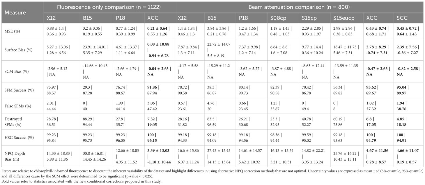
Table 6 Select relative error measures in NPQ corrected chlorophyll fluorescence profiles across different NPQ correction methods, split to show the effect of SCM presence vs. SCM absence (SCM | no SCM) as seen by chlorophyll profiles.

3.6 Considering alternative light thresholds to reduce the errors associated with SCMs

In light of the results presented in Section 3.5, we considered modifications of the P18 method using a range of fractional light thresholds in place of the 1% euphotic depth (Figure 4). The P18 method uses the minimum of either Zeu and MLD as the maximum depth NPQ can be detected (NPQdmax), switching between the X12 and B15 methods in shallow mixing (MLD < Zeu) and deep mixing (MLD > Zeu), respectively. Considering the trade-offs associated with the use of each light threshold, we determine a 20% threshold (Z(rPAR20)) to be the best when considering performance in the presence and absence of an SCM (Figure 4). We refer to the use of Z(rPAR20) in place of MLD as the X12r+ and S08r+ methods. Z(rPAR20) also may be a better indicator than MLD for the minimum depth of SCM formation with 98% of SCMs forming below this depth.

Figure 4

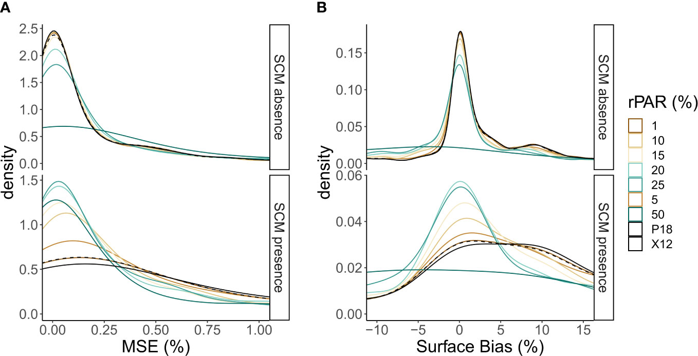
Figure 4 Density distribution plots of (A) mean sum error (MSE) and (B) surface bias, relative to chlorophyll-informed absolute error, when fractional light thresholds (rPAR) are applied to determine the best threshold for X12r+. Density distributions are shown across the presence and absence of SCMs, with reference to the X12 (solid) and P18 (dashed) methods. Diffuse downwelling coefficients for PAR are modelled from Kim et al. (2015).

The optimal adaption of P18 uses the minimum of the MLD and Z(rPAR20) as NPQdmax, switching between the X12 and X12r+ methods in shallow mixing [MLD < Z(rPAR20)] and deep mixing [MLD > Z(rPAR20)], respectively. Using this method still resulted in higher MSE when an SCM was present, however the effect was reduced (Figure 4).

We also considered modifications of the P18 method using modelled absolute thresholds like in X12+ and S08+ (Xing et al., 2018). We interpreted the absolute threshold of 5 or 10 μmol quanta m² s^-1 to be worse compared to using a 20% relative threshold, considering SCM success, MSE and surface bias (Supplementary Figure 2; Supplementary Table 3).

3.7 The case of a freshwater layer from sea-ice melt

We considered 45 cases where a stratified, freshwater layer was detected from recent sea-ice melt, leading to a thin, shallow mixed layer. Using a 20% light threshold within the X12r+ method performs the best under these unique conditions, reducing the MSE, surface chlorophyll bias and SCM chlorophyll bias compared to the X12, S08 and P18 methods (Table 7). Supplementing the method with beam attenuation under these conditions using S08r+ is not favorable and chooses NPQ depths that are much deeper to those observed. Only two SCMs were detected in fresh water layer conditions.

Table 7

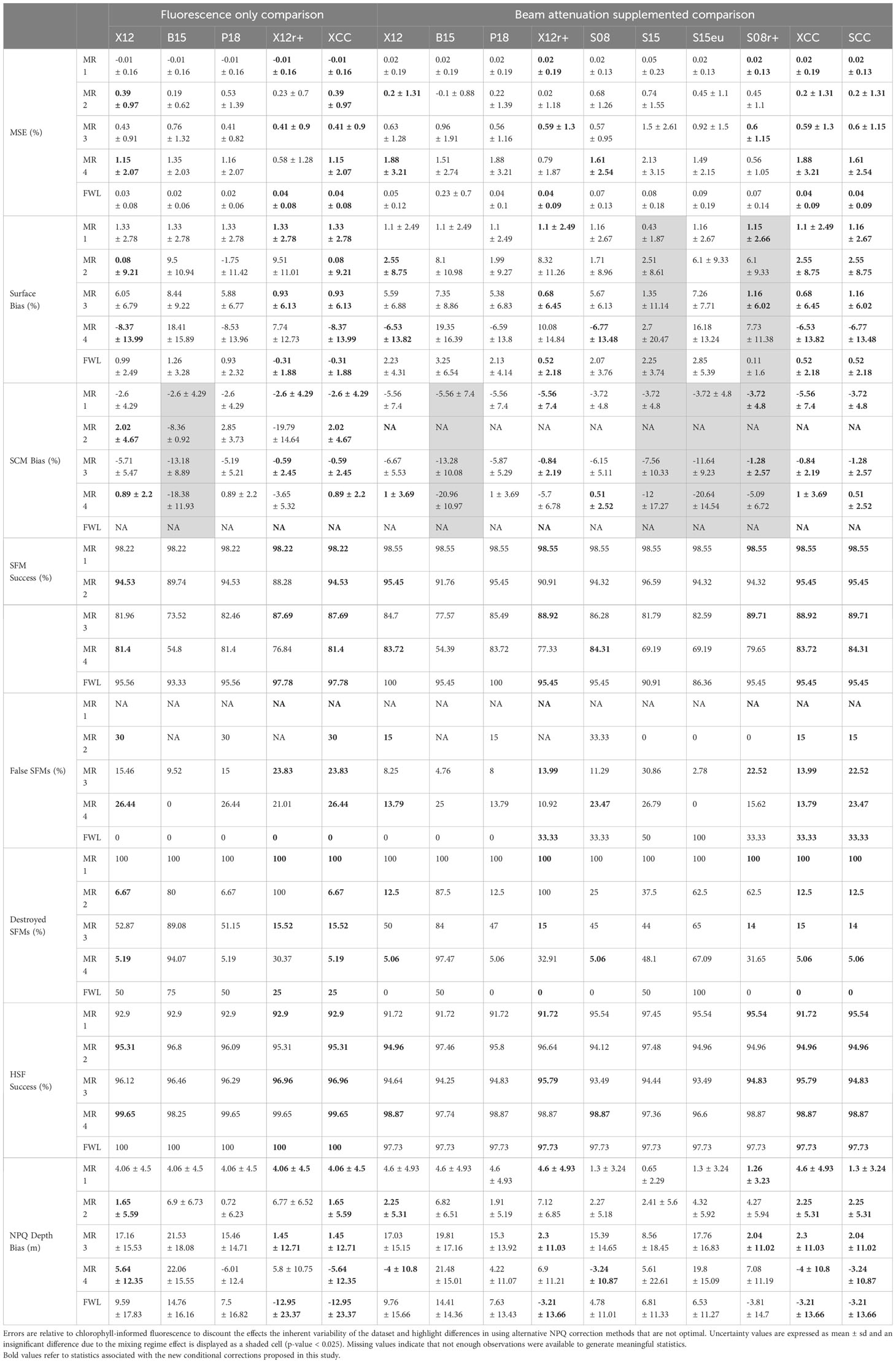
Table 7 Relative error measures in NPQ corrected chlorophyll fluorescence profiles across different NPQ correction methods, split to show the effect of the five mixing regimes (MR 1, MR2, MR3, MR4, FWL).

3.8 A new conditional method reduces errors associated with SCMs

Our findings illustrate that the performance of NPQ correction methods is variable between shallow mixing (MLD < Z(rPAR20)) and deep mixing (MLD > Z(rPAR20)), and in the presence of an SCM. In the absence of chlorophyll data, the position of the SFM in relation to Z(rPAR20) can be used as a coarse indicator for the possibility of a SCM and should be considered when correcting for NPQ (Figure 5).

Figure 5

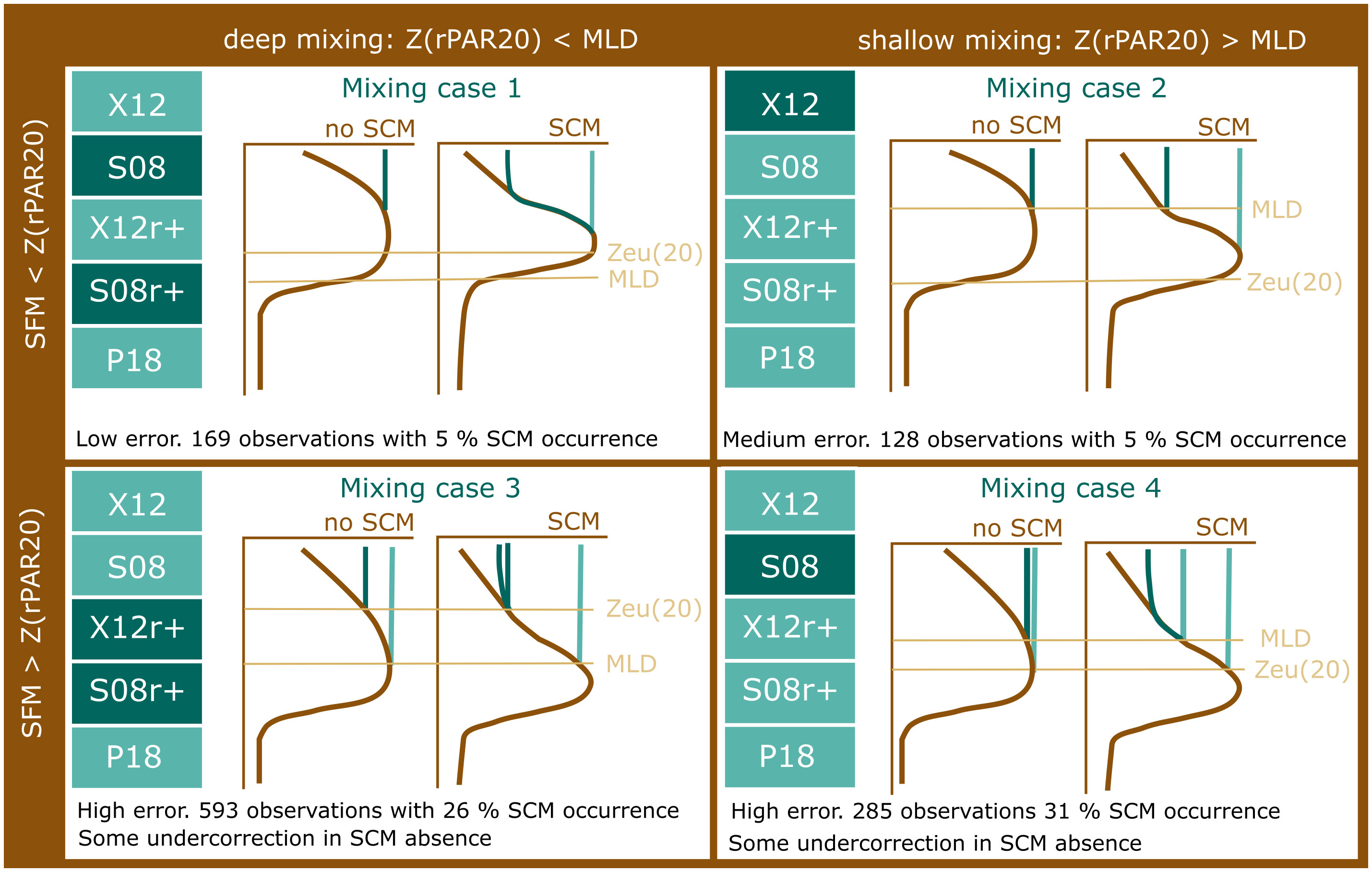
Figure 5 A summary of the results presented in this paper, which lead to the definition of two conditional methods XCC and SCC. We show that the performance of NPQ corrections is reduced when the Z(rPAR20) < SFM and where SCM is observed. Correction methods highlighted in dark were shown to be the best performant methods under each condition. See Table 1 for definitions of the NPQ correction methods shown.

Implementing a 20% light threshold to derive the X12r+ and S08r+ methods, we find that in deep mixing cases and where Z(rPAR20) is deeper than the SCM (mixing case 1), NPQ corrections lead to low average MSE of 0.02 (± 0.13) % and average surface error of 1.16 (± 2.67) in these cases (Table 7). The S08 and S08r+ methods perform the best in this case, when considering MSE, surface chlorophyll bias and SCM chlorophyll bias. There is only a 5% occurrence of SCMs observed in this case. All SFMs detected using chlorophyll-informed methods are destroyed, however the SCM bias is lower when beam attenuation is used to supplement corrections suggesting the partial reconstruction of SCMs. In shallow mixing cases and where Z(rPAR20) is deeper than the SCM (mixing case 2), the X12 method performs the best displaying medium error with average MSE of 0.2 ± (1.31) % and average surface error of 2.55 (± 8.75) %The S08 and P18 methods perform similarly, however they display a higher variability in MSE and surface error. There is only a 5% occurrence of SCMs observed in this case, and beam attenuation supplemented corrections do not appear to replicate SCMs with a higher rate of SCM destruction.

In deep mixing cases and where Z(rPAR20) is shallower than the SFM (mixing case 3), the X12r+ and S08r+ methods significantly outperform the X12, P18 and S08 methods when an SCM is present. Use of the X12r+ and S08r+ methods with an average MSE of 0.6 (± 1.15) %, average surface bias 1.16 ± (6.02) % and average SCM bias of -1.28 ± (2.57) %. Here the effect between the choice of X12r+ and S08r+ is minimal and there is a 26% occurrence of SFMs. Compared to X12, P18 and S08 methods this choice does lead to a higher rate of false SCMs in the absence of real SCMs due to surface underestimation, but the choice of X12r+ and S08r+ reduces the over-correction of X12 in the presence of an SCM and more accurately preserves SFM that are destroyed or suppressed. In shallow mixing cases and where Z(rPAR20) is shallower than the SFM (mixing case 4), the S08 methods performs best with average MSE of 1.61 ± (2.54) %, average surface chlorophyll bias -6.77 ± (13.48) % and average SCM bias of 0.51 ± (2.52) %. This is the highest error of the four mixing cases. The S08 method has the best SFM success rate, SCM bias and MSE compared to X12 and P18, but these latter methods are comparable and minimize the number of false SCMs in the dataset. The X12r+ and S08r+ method underestimates SCM chlorophyll and overestimates surface chlorophyll in this case.

Informed from these results, the best NPQ correction method to implement is the conditional method defined below across five mixing regimes:

Xing Conditional Correction (XCC):

● when the SFM < Z(rPAR20) and the Z(rPAR20) < MLD then use the X12r+ method.

● when the SFM < Z(rPAR20) and the Z(rPAR20) > MLD then use the X12 method.

● when the SFM > Z(rPAR20) and the Z(rPAR20) < MLD then use the X12r+ method.

● when the SFM > Z(rPAR20) and the Z(rPAR20) > MLD then use the X12 method.

● when a FWL is detected use the X12r+ method.

Sackman conditional correction (SCC):

● when the SFM < Z(rPAR20) and the Z(rPAR20) < MLD then use the S08r+ method.

● when the SFM < Z(rPAR20) and the Z(rPAR20) > MLD then use the X12 method.

● when the SFM > Z(rPAR20) and the Z(rPAR20) < MLD then use the S08r+ method.

● when the SFM > Z(rPAR20) and the Z(rPAR20) > MLD then use the S08 method.

● when a FWL is detected use the X12r+ method.

The distribution of these five mixing regimes within the ship and Biogeochemical Argo float datasets are shown in Supplementary Figures 3, 4. Where beam attenuation is available, the SCC method performs the best of all methods when considering the MSE, surface bias, SCM bias and NPQ depth bias. Where beam attenuation data is not available, the XCC method performs the best of all methods when considering the MSE, surface bias and SCM bias (Table 4). The SCC and XCC methods have the highest accuracy of SCM success compared to the S08, X12 and P18 methods and comparable accuracy of HSC success. When considering relative errors to chlorophyll-informed fluorescence, the XCC and SCC methods halve the surface bias, more than halve the SCM chlorophyll bias and have comparable MSE compared to the P18, X12 and S08 methods (Table 4). Notably, the surface and SCM biases are no longer significantly different from chlorophyll-informed fluorescence. The number of destroyed “true” SFMs is much lower compared to any other tested method, but the number of false SCMs due to under-correction is higher than the widely accepted P18, X12 and S08 methods.

To implement these methods in the absence of chlorophyll concentrations, we characterized the sensitivity of the calculation of Z(rPAR20) using Kim et al. (2015) light model to changes in chlorophyll concentration and MLD. We find that the method can be robustly used when the uncertainty in chlorophyll fluorescence slope factor calibration is within a factor of ± 50% fluorescence units to calculate Z(rPAR20) within ± 10 m. Under conditions where the chlorophyll fluorescence slope factor is overestimated (chl-f < chlorophyll concentration), Z(rPAR20) will be calculated deeper and the profile risks being over-corrected, suppressing the relative magnitude of the SCM. This effect becomes apparent when the chlorophyll fluorescence slope factor is underestimated by more than 50% (Supplementary Figures 5, 6). Under conditions where the chlorophyll fluorescence slope factor is underestimated (chl-f > chlorophyll concentration), Z(rPAR20) will be calculated shallower and the risk of under-correction at the surface increases. Higher MSE errors due to NPQ corrections result from when the slope factor is overestimated, versus underestimated.

3.9 The occurrence of NPQ

Using the chlorophyll-informed NPQ correction method, we observe a 35.6% occurrence of NPQ within our dataset. Significant NPQ signals were constrained to the daytime and November/December with sun angles > -5 degrees. 77.0% of NPQ quenching occurred above the 0.03 density MLD and only 50.3% of NPQ quenching occurred above the 20% euphotic depth. These are common depth criteria used within NPQ correction methods. No significant correlation was observed between NPQ depth and sun angle, or NPQ depth and surface chlorophyll.

Applying the SCC method to the BGC-Argo float dataset [Accessed 17/12/2023 and quality assurance applied as in Baldry et al., (in prep)], a 43.3% occurrence of NPQ is observed during day-time (sun angles > -5 degrees) and 3.1% during night-time. The seasonal occurrence of day-time NPQ is highest in December and January (53.1% and 51.6%, respectively) and lowest in June and July (20.1% and 18.9%, respectively). A greater NPQ signal is observed in the dataset around the Polar Front in the eastern sector of the Southern Ocean (Figure 6).

Figure 6

Figure 6 Observations from Biogeochemical Argo profiling floats showing the spatial distribution of (A) the occurrence of significant NPQ and (B) the average NPQ signal observed during day-time (sun angles < -5) derived by applying the SCC correction method across the Southern Ocean. Also shown is (C) the proportion of significant NPQ observed seasonally in the Southern Ocean.

4 Discussion

We have presented a detailed comparison of NPQ methods that finds that the performance of NPQ corrections is worse when an SCM is present, as indicated when the SFM deeper than Z(rPAR20). Conditional methods that consider the position of the MLD, SFM and Z(rPAR20) provide the best methods for correcting chlorophyll fluorescence profiles, building on the methods proposed by Xing et al. (2018). We call these the Xing conditional correction (XCC) and Sackmann conditional correction (SCC) methods, with the implementation of SCC dependent on the availability of beam attenuation or backscatter profiles (Figure 5). Although the XCC and SCC methods have reduced error compared to existing correction methods, particularly when a SCM is present, significant uncertainty in surface chlorophyll still results from correction when Z(rPAR20) is shallower than the SFM - conditions where 98% of SCMs are found.

Our results support previous studies that suggest X12 and S08 over-correct surface chlorophyll from chlorophyll fluorescence in the Southern Ocean (Biermann et al. (2015); Xing et al. (2018); Thomalla et al. (2018)). This over-correction can occur in both “deep mixing” [MLD > Z(rPAR20)] and “shallow mixing” [MLD < Z(rPAR20)] waters due to the presence of SCMs and leads to the suppression of 31.72% (X12) and 27.75% (S08) of real SFMs (Table 4). In the case of “deep mixing”, the most prevalent case in the Southern Ocean, over-correction occurs in the presence of an SCM or real SFM due to the MLD being deeper than the NPQ depth. In this case using Z(rPAR20) instead of MLD in the X12 and S08 methods is more suitable, protecting 98% of SCMs which form below Z(rPAR20). We call these methods X12r+ and S08r+. In the case of “shallow mixing” over-correction by X12 occurs when an SCM is present, associated with a SFM that is deeper than Z(rPAR20) and causes a high chlorophyll fluorescence gradient across the pycnocline. When this SFM is present, correction using X12 leads to increased surface chlorophyll fluorescence and suppresses the relative magnitude of the SFM. Correction can be improved by implementing the S08 method with beam attenuation data, to ensure that SCMs that form under shallow mixing conditions are preserved.

In “shallow mixing” conditions, and where the SFM is deeper than Z(rPAR20), a portion of profiles are under-corrected by X12. These profiles are only corrected by the X12r+ method, but this method has a high rate of destroyed SFMs, resulting in lower chlorophyll at the SCM and over-correction at the surface. The S08r+ method does not perform well in an attempt to preserve the SCM and correct from a deeper depth, possibly due to large changes in beam attenuation properties of phytoplankton below the MLD. Xing et al. (2018) also confirmed this effect with backscatter, noting that when NPQ is deeper than the mixed layer (SFM > MLD, i.e. 100% of mixing case 4 and 56% of mixing case 3) proposed methods cannot retrieve the correct fluorescence chlorophyll, or chlorophyll fluorescence/backscatter ratio, as assumptions that these two quantities are constant below the MLD do not hold.

This artifact is due to the modification of bio-optics within SCMs that form at the pycnocline in the Southern Ocean. We find evidence of this within a following study of SCMs, revealing increased chlorophyll fluorescence yields, increase intracellular chlorophyll and variability in backscatter and beam attenuation yields of phytoplankton around the SCM (Baldry et al. (2020), Baldry et al., (in prep)). Additionally, we could not determine which proxy was most representative of Southern Ocean SCMs due to inconsistencies in the response between the backscatter and beam attenuation yields, where only one of the two proxy yields are suppressed at the SCM (Baldry et al., (in prep)). Finding a solution to NPQ corrections in the presence of an SCM and “shallow mixing” is very necessary as SCMs are widely prevalent in summer under “shallow mixing” and the nutrient-limited conditions that exacerbate NPQ (Baldry et al., (in prep); Falkowski and Kolber (1995); Baldry et al. (2020); Ryan-Keogh and Smith (2021)). Xing et al. (2018) could not propose a suitable method for NPQ correction that eliminates both the underestimation and overestimation of surface chlorophyll in “shallow mixing” conditions. Unfortunately, neither can we without further understanding on the properties of Southern Ocean SCMs and the conditions under which they form.

Thus, like Xing et al. (2018), we find the greatest point of uncertainty for NPQ corrections is the requirement for an alternate method when an SCM is present. In the BGC-Argo dataset there is no ability to delineate between an SCM and NPQ below the MLD or Z(rPAR20). However, our findings are contrary to the concluding remarks of Xing et al. (2018) which stated that the ability to model PAR and apply the 15 μmol quanta m^-2 s^-1 threshold is the greatest source of uncertainty. In fact, the variability in errors between light thresholds is not caused by a consistent NPQ light threshold, but rather variability in the depth of formation of the SCM.

Some confidence can be obtained in our conditional NPQ correction methods, after application of the SCC method to BGC-Argo data. As expected, NPQ is calculated to be small at night-time, suggesting that there may be a small over-correction of real SCMs taken as NPQ signal in the BGC-Argo dataset. Uncertainty in the chlorophyll fluorescence scalar implemented to BGC-Argo (ie. 2 from Roseler et al. (2017) implemented here, versus 3.79 from Schallenberg et al. (2020)) does impact results to a small extent, due to the modelling of Z(rPAR20) within the SCC correction (Supplementary Figure 7). Despite these uncertainties, broad spatial and temporal trends of NPQ can be observed which are not dissimilar to those found from satellite (Behrenfeld et al., 2009). Thus, using the BGC-Argo uncertainties will not largely obscure trends when studying subsurface phytoplankton and SCMs.

5 Conclusions

In this work, we provide an in-depth comparison of NPQ correction methods by comparing corrected chlorophyll fluorescence profiles to coincident chlorophyll concentration measurements from ships. This analysis builds on existing work towards defining best practices by Xing et al. (2018) and Thomalla et al. (2018), who used day-night comparisons of glider and biogeochemical Argo datasets. We provide strong evidence of decreased performance of NPQ algorithms when an SCM is present, due to the overcorrection of chlorophyll fluorescence. We present two conditional methods (SCC and XCC) which improves performance compared to existing methods, however significant deviations from chlorophyll measurements are still observed. This highlights that further characterizing the bio-optics of Southern Ocean SCMs is essential to improving NPQ corrections and the accuracy of surface chlorophyll measurements made by fluorometers. Our study also provides detailed information on how different NPQ corrections impact the retrieval from chlorophyll fluorescence to inform community best practices.

Our current recommendations to inform best practices to compile datasets from chlorophyll fluorescence profiles, that are minimally impacted by the effects of NPQ in the Southern Ocean, are:

● use the SCC method, or the XCC method when beam attenuation or backscatter data is not available.

● when XCC method is used in cases where MLD is deeper than the SFM and the MLD is deeper than Z(rPAR20) note that a high prevalence of fake SCMs could be detected in the dataset. Alternatively, if the X12 method is used in this case a high number of real SCMs will fail to be detected in the dataset.

● when XCC method is used in cases where the MLD is shallower than the SFM, the MLD is shallower than Z(rPAR20) note that a high prevalence of fake SCMs could be detected in the dataset. Alternatively, if the X12r+ method is used in this case a high number of real SCMs will fail to be detected in the dataset.

● use X12r+ when a FWL is detected.

● to only implement modelled Z(rPAR20) when the slope factor is underestimated by less than 50%, or overestimated by less than 50%.

● not to use B15, S15 and S15eu methods.

● if accurate surface measurements are required, use an adapted P18, with Z(rPAR20) in place of Zeu, and remove all profiles with SFMs detected post-correction.

Following our assessment using ship data, we advise the following actions on quality control processes for data being applied to NPQ corrections:

● that smoothed, uncalibrated beam attenuation derived from transmissometers can be used in place of backscatter.

● to use only well understood, smoothed and quality-controlled backscatter and beam attenuation data.

● to shift the local maxima in beam attenuation or backscatter profiles to the depth of the SFM for corrections, if it is detected within 5m of the SFM and there is doubt in the sensor positions.

● to note that high surface chlorophyll conditions cannot be reproduced when profiles are significantly quenched, and surface estimates of chlorophyll from chlorophyll fluorescence will be underestimated in this case.

● to note that changes in chlorophyll fluorescence yield were observed through depth after NPQ correction, which can lead to errors in integrated chlorophyll estimates from chlorophyll fluorescence.

These insights have been offered from a limited dataset of ship-based observations from 61 voyages in the Southern Ocean. In the future, the methods used in this study could yield further insights using biogeochemical Argo float data, replacing chlorophyll concentration measurements with chlorophyll derived from observed diffuse attenuation coefficients (Schallenberg et al. (2022)). In any case, the findings of this paper allow users of chlorophyll fluorescence data to make informed decisions on NPQ corrections and provide optimal chlorophyll-informed method for correction in the presence of co-incident chlorophyll measurements. However, our findings also illustrate the challenges in defining community best practices for the correction of NPQ in chlorophyll fluorescence data and that errors persist in corrected datasets. Thus we suggest that best practices be developed for core applications (e.g. data assimilation into models) based on our findings to minimise errors introduced by NPQ correction inaccuracies.

Data availability statement

Publicly available datasets were analyzed in this study. The data used in this study is freely available through the BIOMATE data compilation (in review). R software (version 3.6.3) was used for all calculations from this source data and to compile the manuscript. Code and resources are available at https://github.com/KimBaldry/NPQ_correction and https://github.com/KimBaldry/Ocean_code. Biogeochemical Argo data is also freely available to use and can be accessed using information available at https://biogeochemical-argo.org/data-access.php. These data were collected and made freely available by the International Argo Program and the national programs that contribute to it. (https://argo.ucsd.edu, https://www.ocean-ops.org). The Argo Program is part of the Global Ocean Observing System [https://doi.org/10.17882/42182]. The quality controlled BGC-Argo dataset which includes profiles of photosynthetically active radiations used within this manuscript is openly available for download (https://doi.org/10.17882/49388).

Author contributions

KB: Conceptualization, Data curation, Investigation, Methodology, Software, Writing – original draft, Writing – review & editing. PS: Supervision, Writing – review & editing. NH: Supervision, Writing – review & editing. PB: Supervision, Writing – review & editing.

Funding

The author(s) declare financial support was received for the research, authorship, and/or publication of this article. This research was supported under Australian Research Council’s Special Research Initiative for Antarctic Gateway Partnership (Project ID SR140300001). It was also partially supported by Geoscience Australia, in the form of paid study leave from employment. NH, PS and PB were supported by the Australian Research Council Special Research Initiative, Australian Centre for Excellence in Antarctic Science (Project Number SR200100008). PS received support from the Australian Research Council Centre of Excellence for Climate Extremes, CE170100023.

Acknowledgments

This research was supported under Australian Research Council’s Special Research Initiative for Antarctic Gateway Partnership (Project ID SR140300001). It was also partially supported by Geoscience Australia, in the form of paid study leave from employment. We acknowledge the use of the BIOMATE data compilation which is only possible because of data made available through following data repositories; PANGAEA, AODN/IMOS, SeaBASS, CCHDO, AADC, GLODAP, PAL-LTER, CSIRO, MDGS and BCO-DMO. Records of data access dates, source addresses and digital object identifiers are recorded as metadata within the compilation, alongside appropriate data citations. We acknowledge the enormous community effort undertaken in the collection, analysis and publication of this data and thank principal investigators for publishing their data in open access repositories. We also acknowledge the use of Biogeochemical Argo data to supplement our discussion. These data were collected and made freely available by the data from the International Argo Program and the national programs that contribute to it. (https://argo.ucsd.edu, https://www.ocean-ops.org). The Argo Program is part of the Global Ocean Observing System [https://doi.org/10.17882/42182]. Finally, we would like to acknowledge support and guidance from Christina Schallenberg in the subject of non-photochemical quenching and fruitful discussions with the participants of the 2019 Bonus-Integral IOCCG Biogeochemical Sensors workshop.

Conflict of interest

The authors declare that the research was conducted in the absence of any commercial or financial relationships that could be construed as a potential conflict of interest.

Publisher’s note

All claims expressed in this article are solely those of the authors and do not necessarily represent those of their affiliated organizations, or those of the publisher, the editors and the reviewers. Any product that may be evaluated in this article, or claim that may be made by its manufacturer, is not guaranteed or endorsed by the publisher.

Supplementary material

The Supplementary Material for this article can be found online at: https://www.frontiersin.org/articles/10.3389/fmars.2023.1302999/full#supplementary-material

Supplementary Figure 1 | Files for Supplementary Figure 1 are available on FigShare: 10.6084/m9.figshare.24995909.

References

Anadón R., Estrada M. (2013a). pH, alkalinity, temperature, salinity and other variables collected from discrete sample and profile observations using CTD, bottle and other instruments from the HESPERIDES in the south atlantic ocean from 1995-12-03 to 1996-01-05 (NCEI accession 0113549) (NOAA National Centers for Environmental Information). doi: 10.3334/cdiac/otg.carina_29he19951203

CrossRef Full Text | Google Scholar

Anadón R., Estrada M. (2013b). pH, alkalinity, temperature, salinity and other variables collected from discrete sample and profile observations using CTD, bottle and other instruments from the HESPERIDES in the south atlantic ocean from 1996-01-17 to 1996-02-05 (NCEI accession 0113755) (NOAA National Centers for Environmental Information). doi: 10.3334/CDIAC/otg.CARINA_29HE19960117

CrossRef Full Text | Google Scholar

Ardyna M., Babin M., Gosselin M., Devred E., Bélanger S., Matsuoka A., et al. (2013). Parameterization of vertical chlorophyll a in the arctic ocean: Impact of the subsurface chlorophyll maximum on regional, seasonal, and annual primary production estimates. Biogeosciences 10 (6), 4383–4404. doi: 10.5194/bg-10-4383-2013

CrossRef Full Text | Google Scholar

Baldry K. (2023). BIOMATE data compilation (v1.0) (University of Tasmania (UTAS: Institute for Marine and Antarctic Studies (IMAS). doi: 10.25959/ETRA-4655

CrossRef Full Text | Google Scholar

Baldry K., Johnson R., Strutton P. G., Hill, Boyd P. W. (in review). BIOMATE: A biological ocean reformatting effort. Nat. Sci. Data.

Google Scholar

Baldry K., Strutton P. G., Hill N. A., Boyd P. W. (2020). Subsurface chlorophyll-a maxima in the southern ocean. Front. Mar. Sci. 7. doi: 10.3389/fmars.2020.00671

CrossRef Full Text | Google Scholar

Baldry K., Tamsitt V., Strutton P. G., Hill N. A., Raymond B., Sumner M., et al. (in prep). Revealing Southern Ocean subsurface chlorophyll maxima with BGC-Argo: Widespread seasonal occurrences, modified surface communities and deep biomass stocks. Journal for Geophysical Research: Oceans.

Google Scholar

Barber R., Chavez F., Coale K. H. (2008). Fluorometric chlorophyll from Niskin and TM bottle samples from R/V Melville, R/V Roger Revelle cruises COOK19MV, DRFT08RR from the Southern Ocean, south of New Zealand in 2002 (SOFeX project) (Biological; Chemical Oceanography Data Management Office (BCO-DMO). Available at: http://lod.bco-dmo.org/id/dataset/2933.

Google Scholar

Behrenfeld M. J., Westberry T. K., Boss E., O’Malley R. T., Siegel D. A., Wiggert J. D., et al. (2009). Satellite-detected fluorescence reveals global physiology of ocean phytoplankton. Biogeosciences 6 (5), 779–794. doi: 10.5194/bg-6-779-2009

CrossRef Full Text | Google Scholar

Bestley S., Rosenberg M. (2019). Aurora Australis Marine Science Cruise AU1603 - Oceanographic Field Measurements and Analysis (AADC). doi: 10.4225/15/5adec86550a1a

CrossRef Full Text | Google Scholar

Bidigare R. (2005a). Pigments, HPLC method, sampled from bottle and TM casts (US JGOFS). Available at: http://usjgofs.whoi.edu/jg/dir/jgofs/southern/nbp96_4A/.

Google Scholar

Bidigare R. (2005b). Pigments, HPLC method, sampled from bottle and TM casts (US JGOFS). Available at: http://usjgofs.whoi.edu/jg/dir/jgofs/southern/nbp97_1/.

Google Scholar

Bidigare R. (2005c). Pigments, HPLC method, sampled from bottle and TM casts (US JGOFS). Available at: http://usjgofs.whoi.edu/jg/dir/jgofs/southern/nbp97_3/.

Google Scholar

Bidigare R. (2005d). Pigments, HPLC method, sampled from bottle and TM casts (US JGOFS). Available at: http://usjgofs.whoi.edu/jg/dir/jgofs/southern/nbp97_8/.

Google Scholar

Bidigare R., Landry M. R. (2007). Pigments from HPLC analysis of bottle samples from SOFeX cruisse PS02_2002, COOK19MV, DRFT08RR from the Southern Ocean, south of New Zealand, Southern Ocean in 2002 (SOFeX project) (Biological; Chemical Oceanography Data Management Office (BCO-DMO). Available at: http://lod.bco-dmo.org/id/dataset/2818.

Google Scholar

Biermann L., Guinet C., Bester M., Brierley A., Boehme L. (2015). An alternative method for correcting fluorescence quenching. Ocean Sci. 11 (1), 83–91. doi: 10.5194/os-11-83-2015

CrossRef Full Text | Google Scholar

Boss E., Talley L. (2020a). CLIVAR (Greenbelt, Maryland: SeaBASS). doi: 10.5067/SeaBASS/CLIVAR/DATA001

CrossRef Full Text | Google Scholar

Boss E., Talley L. (2020b). SOCCOM HPLC pigments (SeaBASS). doi: 10.5067/SeaBASS/SOCCOM/DATA001

CrossRef Full Text | Google Scholar

Bracher A. (2014). Phytoplankton pigment concentrations during POLARSTERN cruise ANT-XXVIII/3 (PANGAEA: Alfred Wegener Institute, Helmholtz Centre for Polar; Marine Research, Bremerhaven). doi: 10.1594/PANGAEA.848588

CrossRef Full Text | Google Scholar

Bracher A. (2019). Phytoplankton pigment concentrations in the Southern Ocean during RV POLARSTERN cruise PS103 in Dec 2016 to Jan 2017 (PANGAEA: Alfred Wegener Institute, Helmholtz Centre for Polar; Marine Research, Bremerhaven). doi: 10.1594/PANGAEA.898941

CrossRef Full Text | Google Scholar

Buesseler K. O., Coale K. H., Siegel D. (2007). USCGC Polar Star cruises COOK19MV, DRFT08RR, PS02_2002 from the Southern Ocean, south of New Zealand in 2002 (SOFeX project) (Biological; Chemical Oceanography Data Management Office (BCO-DMO). Available at: http://lod.bco-dmo.org/id/dataset/2851.

Google Scholar

Byrd R. H., Lu P., Nocedal J., Zhu C. (1995). A limited memory algorithm for bound constrained optimization. SIAM J. Sci. computing 16 (5), 1190–1208. doi: 10.1137/0916069

CrossRef Full Text | Google Scholar

Carbotte S. M., Ryan W. B. F., O’Hara S., Arko R., Goodwillie A., Melkonian A., et al. (2007). Antarctic Multibeam Bathymetry and Geophysical Data Synthesis: An On-Line Digital Data Resource for Marine Geoscience Research in the Southern Ocean (U.S. Geological Survey Open-File Report 2007-1047). doi: 10.3133/of2007-1047.srp002

CrossRef Full Text | Google Scholar

Carranza M. M., Gille S. T., Franks P. J. S., Johnson K. S., Pinkel R., Girton J. B. (2018). When mixed layers are not mixed. Storm-driven mixing and bio-optical vertical gradients in mixed layers of the southern ocean. J. Geophysical Research: Oceans 123 (10), 7264–7289. doi: 10.1029/2018JC014416

CrossRef Full Text | Google Scholar

Carvalho F., Kohut J., Oliver M. J., Schofield O. (2017). Defining the ecologically relevant mixed-layer depth for Antarctica’s coastal seas. Geophysical Res. Lett. 44 (1), 338–345. doi: 10.1002/2016GL071205

CrossRef Full Text | Google Scholar

Claustre H. (2013). HPLC pigments from TARA oceans expedition analysed at LOV (SeaBASS). doi: 10.1594/PANGAEA.836321

CrossRef Full Text | Google Scholar

Claustre H., Johnson K. S., Takeshita Y. (2020). Observing the global ocean with biogeochemical-argo. Annu. Rev. Mar. Sci. 12 (1), 23–48. doi: 10.1146/annurev-marine-010419-010956

CrossRef Full Text | Google Scholar

Clementson L. (2020a). Franklin cruise 10/97 HPLC Pigment and Ocean Colour Data (IMOS). Available at: https://portal.aodn.org.au/search?uuid=97b9fe73-ee44-437f-b2ae-5b8613f81042.

Google Scholar

Clementson L. (2020b). Southern Surveyor Voyage SS 03/96 HPLC Pigment and Ocean Colour Data (IMOS). Available at: https://portal.aodn.org.au/search?uuid=97b9fe73-ee44-437f-b2ae-5b8613f81042.

Google Scholar

Clementson L. (2020c). Southern Surveyor Voyage SS2010_V09 HPLC Pigment and Ocean Colour Data (IMOS). Available at: https://portal.aodn.org.au/search?uuid=97b9fe73-ee44-437f-b2ae-5b8613f81042.

Google Scholar

Clementson L. (2020d). SRFME Ocean Colour data - OffShore, Southern Surveyor SS 01/2004 (IMOS). Available at: https://portal.aodn.org.au/search?uuid=97b9fe73-ee44-437f-b2ae-5b8613f81042.

Google Scholar

Cornec M., Claustre H., Mignot A., Guidi L., Lacour L., Poteau A., et al. (2021). Deep chlorophyll maxima in the global ocean: Occurrences, drivers and characteristics. Global Biogeochemical Cycles 35 (4), e2020GB006759. doi: 10.1029/2020GB006759

CrossRef Full Text | Google Scholar

CSIRO (1998). Southern Surveyor Voyage SS 03/96 CTD Data (CSIRO). Available at: https://marlin.csiro.au/geonetwork/srv/eng/catalog.search#/metadata/900e2c7e-b0d2-4740-a458-8503a5340de7.

Google Scholar

CSIRO (1999). Franklin voyage FR 10/97 CTD data (CSIRO). Available at: https://www.marine.csiro.au/data/trawler/dataset.cfm?survey=FR199710&data_type=ctd.

Google Scholar

CSIRO (2000). Southern Surveyor Voyage SS 01/2004 CTD Data (CSIRO). Available at: https://marlin.csiro.au/geonetwork/srv/eng/catalog.search#/metadata/dc42f374-b762-4bea-956a-f44a6cda956e.

Google Scholar

CSIRO (2012). Southern Surveyor Voyage SS2010_V09 CTD Data (CSIRO). Available at: https://marlin.csiro.au/geonetwork/srv/eng/catalog.search#/metadata/bc1b3741-e7d9-5039-e044-00144f7bc0f4.

Google Scholar

CSIRO (2016). RV Investigator Voyage IN2016_V03 CTD Data (CSIRO). Available at: https://marlin.csiro.au/geonetwork/srv/eng/catalog.search#/metadata/d57331f4-3213-4817-b47e-a2ad0292148a.

Google Scholar

Davies C. H., Ajani P., Armbrecht L., Atkins N., Baird M. E., Beard J., et al. (2018). A database of chlorophyll a in Australian waters. Sci. Data 5 (1), 1–8. doi: 10.1038/sdata.2018.18

CrossRef Full Text | Google Scholar

de Villiers S., Siswana K., Vena K. (2015). Hydrography and biogeochemistry during S.A. Agulhas II cruise Agu011, in the SW Indian Ocean, April 2014 (PANGAEA). doi: 10.1594/PANGAEA.848875

CrossRef Full Text | Google Scholar

Falkowski P., Kolber Z. (1995). Variations in chlorophyll fluorescence yields in phytoplankton in the world oceans. Funct. Plant Biol. 22 (2), 341–355. doi: 10.1071/PP9950341

CrossRef Full Text | Google Scholar

García M. A., Castro C. G., Ríos A. F., Doval M. D., Rosón G., Gomis D., et al. (2002a). Physical oceanography during Hespérides cruise Fruela95 (PANGAEA). doi: 10.1594/PANGAEA.825643

CrossRef Full Text | Google Scholar

García M. A., Castro C. G., Ríos A. F., Doval M. D., Rosón G., Gomis D., et al. (2002b). Physical oceanography during Hespérides cruise Fruela96 (PANGAEA). doi: 10.1594/PANGAEA.825644

CrossRef Full Text | Google Scholar

Goericke R. (2005). Pigments, HPLC method, sampled from bottle casts (US JGOFS). Available at: http://usjgofs.whoi.edu/jg/dir/jgofs/southern/rr-kiwi_6/.

Google Scholar

Gregory M. B. (2015). Calibrated Hydrographic Data acquired with a CTD from the Scotia Sea, Antarctica acquired during the Nathaniel B. Palmer expedition NBP0606 (Interdisciplinary Earth Data Alliance). doi: 10.1594/IEDA/321960

CrossRef Full Text | Google Scholar

Gregory M. B. (2016). Measurements taken in the Blue Water Zone (BWZ) under NSF funding near Antarctica and Drakes Passage in 2004 to 2006 (SeaBASS). doi: 10.5067/SeaBASS/NSF-BWZ/DATA001

CrossRef Full Text | Google Scholar

Guinet C., Xing X., Walker E., Monestiez P., Marchand S., Picard B., et al. (2013). Calibration procedures and first dataset of southern ocean chlorophyll a profiles collected by elephant seals equipped with a newly developed CTD-fluorescence tags. Earth System Sci. Data 5 (1), 15–29. doi: 10.5194/essd-5-15-2013

CrossRef Full Text | Google Scholar

Haëntjens N., Boss E., Talley L. D. (2017). Revisiting ocean color algorithms for chlorophyll a and particulate organic carbon in the southern ocean using biogeochemical floats. J. Geophysical Research: Oceans 122 (8), 6583–6593. doi: 10.1002/2017JC012844

CrossRef Full Text | Google Scholar

Hemsley V. S., Smyth T. J., Martin A. P., Frajka-Williams E., Thompson A. F., Damerell G., et al. (2015). Estimating oceanic primary production using vertical irradiance and chlorophyll profiles from ocean gliders in the north atlantic. Environ. Sci. Technol. 49 (19), 11612–11621. doi: 10.1021/acs.est.5b00608

CrossRef Full Text | Google Scholar

Iannuzzi R. (2018). Conductivity Temperature Depth (CTD) sensor profile data binned by depth from PAL LTER annual cruises 1991 - 2017 (ongoing) (Palmer Station Antarctica LTER). doi: 10.6073/pasta/12276fbc0d68568177702aed0d4b44bc

CrossRef Full Text | Google Scholar

Katsumata K. (2015). CTD data from cruise 49NZ20121128 (CCHDO). Available at: https://cchdo.ucsd.edu/cruise/49NZ20121128.

Google Scholar

Katsumata K., Murata A., Uchida H., Aoyama M., Kumamoto Y., Aoki S. (2016). Dissolved inorganic carbon (DIC), pH on total scale, total alkalinity, temperature, salinity and other variables collected from discrete samples and profile observations during the r/v mirai cruise GO-SHIP_P14S_S04_2012; MR12-05 leg 2 (EXPOCODE 49NZ20121128) in the Indian, south pacific and southern oceans from 2012-11-28 to 2013-01-04 (NCEI accession 0143950) (NOAA National Centers for Environmental Information). doi: 10.3334/cdiac/otg.goship_p14s_s04_2012

CrossRef Full Text | Google Scholar

Key R. M., Olsen A., Heuven S., Lauvset S. K., Velo A., Lin X., et al. (2015). Global Ocean Data Analysis Project, Version 2 (GLODAPv2), ORNL/CDIAC-162, ND-P093. Oak Ridge, Tennessee: Carbon Dioxide Information Analysis Center, Oak Ridge National Laboratory, US Department of Energy. doi: 10.3334/CDIAC/OTG.NDP093_GLODAPv2

CrossRef Full Text | Google Scholar

Kim G. E., Pradal M.-A., Gnanadesikan A. (2015). Quantifying the biological impact of surface ocean light attenuation by colored detrital matter in an ESM using a new optical parameterization. Biogeosciences 12 (16), 5119–5132. doi: 10.5194/bg-12-5119-2015

CrossRef Full Text | Google Scholar

Lavigne H., D’Ortenzio F., Ribera D’Alcalà M., Claustre H., Sauzède R., Gacic M. (2015). On the vertical distribution of the chlorophyll a concentration in the mediterranean sea: A basin-scale and seasonal approach. Biogeosciences 12 (16), 5021–5039. doi: 10.5194/bg-12-5021-2015

CrossRef Full Text | Google Scholar

Macdonald A. (2016). ctd data from cruise 33RR20160208 (CCHDO). doi: 10.7942/C2H59N

CrossRef Full Text | Google Scholar

Meyer B., Freier U., Grimm V., Groeneveld J., Hunt B. P. V., Kerwath S., et al. (2017). Chorophyll a and particulate organic carbon measured on water bottle samples during POLARSTERN cruise ANT-XXIX/7 (PANGAEA). doi: 10.1594/PANGAEA.864704

CrossRef Full Text | Google Scholar

Meyer B., Rohardt G. (2014). Physical oceanography during POLARSTERN cruise ANT-XXIX/7 (Alfred Wegener Institute, Helmholtz Centre for Polar; Marine Research, Bremerhaven: PANGAEA). doi: 10.1594/PANGAEA.836537

CrossRef Full Text | Google Scholar

Morison J. (2005a). Final CTD data, including beam attenuation optics (US JGOFS). Available at: http://usjgofs.whoi.edu/jg/dir/jgofs/southern/rr-kiwi_6/.

Google Scholar

Morison J. (2005b). Final CTD data, including beam attenuation optics (US JGOFS). Available at: http://usjgofs.whoi.edu/jg/dir/jgofs/southern/rr-kiwi_7/.

Google Scholar

Morison J. (2005c). Final CTD data, including beam attenuation optics (US JGOFS). Available at: http://usjgofs.whoi.edu/jg/dir/jgofs/southern/rr-kiwi_8/.

Google Scholar

Morison J. (2005d). Final CTD data, including beam attenuation optics (US JGOFS). Available at: http://usjgofs.whoi.edu/jg/dir/jgofs/southern/rr-kiwi_9/.

Google Scholar

Morrison J. (2005a). Final version CTD, including beam attenuation optics (US JGOFS). Available at: http://usjgofs.whoi.edu/jg/dir/jgofs/southern/nbp96_4A/.

Google Scholar

Morrison J. (2005b). Final version CTD, including beam attenuation optics (US JGOFS). Available at: http://usjgofs.whoi.edu/jg/dir/jgofs/southern/nbp97_1/.

Google Scholar

Morrison J. (2005c). Final version CTD, including beam attenuation optics (US JGOFS). Available at: http://usjgofs.whoi.edu/jg/dir/jgofs/southern/nbp97_3/.

Google Scholar

Morrison J. (2005d). Final version CTD, including beam attenuation optics (US JGOFS). Available at: http://usjgofs.whoi.edu/jg/dir/jgofs/southern/nbp97_8/.

Google Scholar

Morrison J. (2005e). Final version CTD, including beam attenuation optics (US JGOFS). Available at: http://usjgofs.whoi.edu/jg/dir/jgofs/southern/nbp98_2/.

Google Scholar

Olsen A., Key R. M., Heuven S., Lauvset S. K., Velo A., Lin X., et al. (2016). The global ocean data analysis project version 2 (GLODAPv2) – an internally consistent data product for the world ocean. Earth System Sci. Data 8 (2), 297–323. doi: 10.5194/essd-8-297-2016

CrossRef Full Text | Google Scholar

Peeken I., Hoffmann L. (2014). Phytoplankton pigments in surface water during POLARSTERN cruise ANT-XXI/3 (EIFEX) (PANGAEA). doi: 10.1594/PANGAEA.869825

CrossRef Full Text | Google Scholar

Peeken I., Nachtigall K. (2014). Pigments in surface water during POLARSTERN cruise ANT-XXVI/3 (PANGAEA). doi: 10.1594/PANGAEA.869827

CrossRef Full Text | Google Scholar

Photopoulou T., Lovell P., Fedak M. A., Thomas L., Matthiopoulos J. (2015). Efficient abstracting of dive profiles using a broken-stick model. Methods Ecol. Evol. 6 (3), 278–288. doi: 10.1111/2041-210X.12328

CrossRef Full Text | Google Scholar

Picheral M., Searson S., Taillandier V., Bricaud A., Boss E., Stemmann L., et al. (2014). Vertical profiles of environmental parameters measured from physical, optical and imaging sensors during Tara Oceans expedition 2009-2013 (PANGAEA). doi: 10.1594/PANGAEA.836321

CrossRef Full Text | Google Scholar

Rintoul S., Rosenberg M. (2004). Aurora Australis marine science cruise au0103 (CLIVAR_SR3) - CTD and ADCP data (AADC). doi: 10.4225/15/58a5360c6c0db

CrossRef Full Text | Google Scholar

Rintoul S., Rosenberg M., Bindoff N., Church J., Yasushi F. (2004). Kerguelen Plateau Deep Western Boundary Current Experiment (DWBC), Aurora Australis marine science cruise au0304 - ship-based CTD, ADCP and LADCP data (AADC). doi: 10.4225/15/58ad0bd50bd58

CrossRef Full Text | Google Scholar

Rohardt G., Boebel O. (2017). Physical oceanography during POLARSTERN cruise PS103 (ANT-XXXII/2) (Alfred Wegener Institute, Helmholtz Centre for Polar; Marine Research, Bremerhaven: PANGAEA). doi: 10.1594/PANGAEA.881076

CrossRef Full Text | Google Scholar

Roquet F., Charrassin J.-B., Marchand S., Boehme L., Fedak M. A., Reverdin G., et al. (2011). Delayed-mode calibration of hydrographic data obtained from animal-borne satellite relay data loggers. J. Atmospheric Oceanic Technol. 28 (6), 787–801. doi: 10.1175/2010JTECHO801.1

CrossRef Full Text | Google Scholar

Roesler C., Uitz J., Claustre H., Boss E., Xing X., Organelli E., et al (2017). Recommendations for obtaining unbiased chlorophyll estimates from in situ chlorophyll fluorometers: A global analysis of WET Labs ECO sensors. Limnology and Oceanography: Methods 15 (6), 572-585.

Google Scholar

Rosenberg M. (2020). Aurora Australis Southern Ocean oceanographic data, voyage 6, 2000-2001 - KACTAS (AADC). doi: 10.26179/5e7411e49faf2

CrossRef Full Text | Google Scholar

Rosenberg M., Gorton R. (2019). BROKE West Survey, Marine Science Cruise AU0603 - Oceanographic Field Measurements and Analysis (AADC). doi: 10.26179/5ceb6d79c35a4

CrossRef Full Text | Google Scholar

Rosenberg M., Howard W., Griffiths B. (2010). CTD data collected during the SAZ-SENSE voyage, January-February 2007 (AADC). doi: 10.4225/15/57B13F22B2F87

CrossRef Full Text | Google Scholar

Rosenberg M., Rintoul S. (2019). Southern Ocean CTD data collected from the CASO cruise of the Aurora Australis (AADC). doi: 10.4225/15/58ad18180df56

CrossRef Full Text | Google Scholar

Rosenberg M., Ronai B. (2005). Database of CTD data collected in the Southern Ocean by the AAD, ACE CRC and part of the Southern Ocean Atlas data set., Ver. 1 (AADC). doi: 10.4225/15/58afb50245d5c

CrossRef Full Text | Google Scholar

Ryan-Keogh T. J., Smith W. O. (2021). Temporal patterns of iron limitation in the ross sea as determined from chlorophyll fluorescence. J. Mar. Syst. 215, 103500. doi: 10.1016/j.jmarsys.2020.103500

CrossRef Full Text | Google Scholar

Ryan-Keogh T. J., Thomalla S. J. (2020). Deriving a proxy for iron limitation from chlorophyll fluorescence on buoyancy gliders. Front. Mar. Sci. 7. doi: 10.3389/fmars.2020.00275

CrossRef Full Text | Google Scholar

Ryan-Keogh T. J., Thomalla S. J., Monterio P. M., Tagliabue A. (2023). Multidecadal trend of increasing iron stress in Southern Ocean phytoplankton. Science 379, 6634. doi: 10.1126/science.abl5237

CrossRef Full Text | Google Scholar

Sackmann B. S., Perry M. J., Eriksen C. C. (2008). Seaglider observations of variability in daytime fluorescence quenching of chlorophyll-a in northeastern pacific coastal waters. Biogeosciences Discussions 5, 2839–2865. doi: 10.5194/bgd-5-2839-2008

CrossRef Full Text | Google Scholar

Schallenberg C., Strzepek R. F., Bestley S., Wojtasiewicz B., Trull T. W. (2022). Iron limitation drives the globally extreme fluorescence/chlorophyll ratios of the southern ocean. Geophysical Res. Lett. 49 (12), e2021GL097616. doi: 10.1029/2021GL097616

CrossRef Full Text | Google Scholar

Schallenberg C., Strzepek R. F., Schuback N., Clementson L. A., Boyd P. W., Trull T. W. (2020). Diel quenching of southern ocean phytoplankton fluorescence is related to iron limitation. Biogeosciences 17 (3), 793–812. doi: 10.5194/bg-17-793-2020

CrossRef Full Text | Google Scholar

Schofield O., Prezelin B., Vernet M. (2018). Photosynthetic pigments of water column samples and analyzed with High Performance Liquid Chromatography (HPLC), collected aboard Palmer LTER annual cruises off the coast of the Western Antarctica Peninsula 1991 - 2016 (Palmer Station Antarctica LTER). doi: 10.6073/pasta/4d583713667a0f52b9d2937a26d0d82e

CrossRef Full Text | Google Scholar

Schofield O., Smith R., Vernet M. (2020). Chlorophyll and phaeopigments from water column samples, collected at selected depths aboard Palmer LTER annual cruises off the coast of the Western Antarctic Peninsula 1991 – 2019 (Palmer Station Antarctica LTER). doi: 10.6073/pasta/6bbce1e3264571463c0354874dba88cf

CrossRef Full Text | Google Scholar

Schröder M., Wisotzki A. (2010). Physical oceanography during POLARSTERN cruise ANT-XXVI/3 (Alfred Wegener Institute, Helmholtz Centre for Polar; Marine Research, Bremerhaven: PANGAEA). doi: 10.1594/PANGAEA.754248

CrossRef Full Text | Google Scholar

Sloyan B. M., Swift J. (2017). ctd data from cruise 33RR200501 (CCHDO). Available at: https://cchdo.ucsd.edu/cruise/33RR200501.

Google Scholar

Smetacek V., de Baar H. J. W., Bathmann U., Lochte K., Rutgers van der Loeff M. M. (1997a). Physical oceanography during POLARSTERN cruise ANT-X/6 (PANGAEA). doi: 10.1594/PANGAEA.759261

CrossRef Full Text | Google Scholar

Smetacek V., de Baar H. J. W., Bathmann U., Lochte K., Rutgers van der Loeff M. M. (1997b). Pigments measured on water bottle samples during POLARSTERN cruise ANT-X/6 (PANGAEA). doi: 10.1594/PANGAEA.761047

CrossRef Full Text | Google Scholar

Smith W. O. (2005a). Fluorometric chlorophyll-a (US JGOFS). Available at: http://usjgofs.whoi.edu/jg/dir/jgofs/southern/rr-kiwi_7/.

Google Scholar

Smith W. O. (2005b). Fluorometric chlorophyll-a (US JGOFS). Available at: http://usjgofs.whoi.edu/jg/dir/jgofs/southern/rr-kiwi_8/.

Google Scholar

Smith W. O. (2005c). Fluorometric chlorophyll-a (US JGOFS). Available at: http://usjgofs.whoi.edu/jg/dir/jgofs/southern/rr-kiwi_9/.

Google Scholar

Smith W. O. (2005d). Fluorometric chlorophyll-a & phaeopigments (US JGOFS). Available at: http://usjgofs.whoi.edu/jg/dir/jgofs/southern/nbp98_2/.

Google Scholar

Smith W. O. (2008). Uncalibrated Hydrographic Data aquired with a CTD in the Ross Sea during the Nathaniel B. Palmer expedition NBP0601A (Interdisciplinary Earth Data Alliance (IEDA). doi: 10.1594/IEDA/305330

CrossRef Full Text | Google Scholar

Smith W. O. (2017). Bottle data including phosphate, nitrate, total nitrite and nitrate, ammonium, silicate, chlorophyll, particulate organic carbon and nitrogen (POC, PON), and biogenic silica from multiple cruises to the southern Ross Sea 2001-2006 (IVARS project) (Biological; Chemical Oceanography Data Management Office (BCO-DMO). doi: 10.26008/1912/bco-dmo.710112.1

CrossRef Full Text | Google Scholar

Strass V. H. (2010). Physical oceanography during POLARSTERN cruise ANT-XXI/3 (EIFEX) (Alfred Wegener Institute, Helmholtz Centre for Polar; Marine Research, Bremerhaven: PANGAEA). doi: 10.1594/PANGAEA.733410

CrossRef Full Text | Google Scholar

Strass V. H., Leach H., Prandke H., Donnelly M., Bracher A., Wolf-Gladrow D. A. (2016). Physical oceanography during POLARSTERN cruise ANT-XXVIII/3 (PANGAEA). doi: 10.1594/PANGAEA.840334

CrossRef Full Text | Google Scholar

Swart S., Thomalla S. J., Monteiro P. M. S. (2015). The seasonal cycle of mixed layer dynamics and phytoplankton biomass in the sub-antarctic zone: A high-resolution glider experiment. J. Mar. Syst. 147, 103–115. doi: 10.1016/j.jmarsys.2014.06.002

CrossRef Full Text | Google Scholar

Swift J. (2017). CTD data from 320620110219 (CCDHO). Available at: https://cchdo.ucsd.edu/cruise/320620110219.

Google Scholar

Talley L. (2017). CTD data from 320620140320 (CCDHO). doi: 10.7942/320620140320

CrossRef Full Text | Google Scholar

Thomalla S. J., Moutier W., Ryan-Keogh T. J., Gregor L., Schütt J. (2018). An optimized method for correcting fluorescence quenching using optical backscattering on autonomous platforms. Limnology Oceanography: Methods 16 (2), 132–144. doi: 10.1002/lom3.10234

CrossRef Full Text | Google Scholar

Uchida H. (2015). CTD data from cruise 49NZ20130106 (CCHDO). Available at: https://cchdo.ucsd.edu/cruise/49NZ20130106.

Google Scholar

Uchida H. (2018). CTD data from cruise 49NZ20170208 (CCHDO). Available at: https://cchdo.ucsd.edu/cruise/49NZ20170208.

Google Scholar

Uchida H., Murata A., Aoyama M., Kumamoto Y., Aoki S. (2016). Dissolved inorganic carbon (DIC), pH on total scale, total alkalinity, temperature, salinity and other variables collected from discrete sample and profile observations obtained during the r/v mirai cruise GOSHIP_S04I_2013 (EXPOCODE 49NZ20130106) in the Indian ocean and southern oceans from 2013-01-06 to 2013-02-15 (NCEI accession 0156925) (NOAA National Centers for Environmental Information). doi: 10.3334/CDIAC/OTG.GOSHIP_S04I_2013

CrossRef Full Text | Google Scholar

Werdell P. J., Bailey S. (2002). The SeaWiFS bio-optical archive and storage system (SeaBASS): Current architecture and implementation. Eds. Fargion G. S., McClain C. R. (Greenbelt, Maryland: NASA Goddard Space Flight Center).

Google Scholar

Werdell P. J., Bailey S., Fargion G., Pietras C., Knobelspiesse K., Feldman G., et al. (2003). Unique data repository facilitates ocean color satellite validation. Eos Trans. Am. Geophysical Union 84 (38), 377–387. doi: 10.1029/2003EO380001

CrossRef Full Text | Google Scholar

William R. H., Griffiths B. (2014). Samples collected for HPLC pigments, microscopy and flow cytometry for the SAZ-SENSE project (AADC). doi: 10.4225/15/556E63D646382

CrossRef Full Text | Google Scholar

Wright S. (2010). The role of Antarctic marine protists in trophodynamics and global change and the impact of UV-B on these organisms - Voyage 3, BROKE-West, Aurora Australis 2005/2006 samples (AADC). doi: 10.4225/15/528C426A13819

CrossRef Full Text | Google Scholar

Wright S. (2013a). Chlorophyll a data collected on voyage 3 of the Aurora Australis in the 2002-2002 season - CLIVAR (Climate Variability) voyage (AADC). doi: 10.4225/15/5212D592E3ED9

CrossRef Full Text | Google Scholar

Wright S. (2013b). The role of Antarctic marine protists in trophodynamics and global change and the impact of UV-B on these organisms - HIPPIES samples, Ver. 1, (AADC). doi: 10.4225/15/52845DCD3AD19

CrossRef Full Text | Google Scholar

Wright S. (2013c). The role of Antarctic marine protists in trophodynamics and global change and the impact of UV-B on these organisms - KACTAS samples (AADC). doi: 10.4225/15/5212CDBC6EC44

CrossRef Full Text | Google Scholar

Wright S. (2013d). The role of Antarctic marine protists in trophodynamics and global change and the impact of UV-B on these organisms - Voyage 4 2002/2003 samples (KAOS) (AADC). doi: 10.4225/15/521412D6095CA

CrossRef Full Text | Google Scholar

Wright S. (2013e). The role of Antarctic marine protists in trophodynamics and global change and the impact of UV-B on these organisms - Voyage 6, Aurora Australis 2007/2008 samples (AADC). doi: 10.4225/15/5292DD6705559

CrossRef Full Text | Google Scholar

Xing X., Briggs N., Boss E., Claustre H. (2018). Improved correction for non-photochemical quenching of in situ chlorophyll fluorescence based on a synchronous irradiance profile. Opt. Express 26 (19), 24734–24751. doi: 10.1364/OE.26.024734

CrossRef Full Text | Google Scholar

Xing X., Claustre H., Blain S., D’Ortenzio F., Antoine D., Ras J., et al. (2012). Quenching correction for in vivo chlorophyll fluorescence acquired by autonomous platforms: A case study with instrumented elephant seals in the kerguelen region (southern ocean). Limnology Oceanography: Methods 10 (7), 483–495. doi: 10.4319/lom.2012.10.483

CrossRef Full Text | Google Scholar