Predicting rapid intensification of tropical cyclones in the western North Pacific: a machine learning and net energy gain rate approach

In this study, a machine learning (ML)-based Tropical Cyclones (TCs) Rapid Intensification (RI) prediction model has been developed by using the Net Energy Gain Rate Index (NGR). This index realistically captures the energy exchanges between the ocean and the atmosphere during the intensification of TCs. It does so by incorporating the thermal conditions of the upper ocean and using an accurate parameterization for sea surface roughness. To evaluate the effectiveness of NGR in enhancing prediction accuracy, five distinct ML algorithms were utilized: Decision Tree, Logistic Regression, Support Vector Machine, K-Nearest Neighbors, and Feed-forward Neural Network. Two sets of experiments were performed for each algorithm. The first set used only traditional predictors, while the second set incorporated NGR. The outcomes revealed that models trained with the inclusion of NGR exhibited superior performance compared to those that only used traditional predictors. Additionally, an ensemble model was developed by utilizing a hard-voting method, combining the predictions of all five individual algorithms. This ensemble approach showed a noteworthy improvement of approximately 10% in the skill score of RI prediction when NGR was included. The findings of this study emphasize the potential of NGR in refining TC intensity prediction and underline the effectiveness of ensemble ML models in RI event detection.

1 Introduction

Tropical cyclones (TCs), as one of the most devastating natural hazards in the world, have caused huge social, and economic damage and loss of life. The recent global TC activity showed a significant increasing trend in major TCs, rapid intensification (RI) events, and TC-induced damage (Balaguru et al., 2018; Kossin et al., 2020; Klotzbach et al., 2022). Many studies have warned the possible serious disasters due to the increase in the very intense TC frequency above category 4 and lifetime maximum intensity, with human-induced climate change (Murakami et al., 2013; Knutson et al., 2020). To reduce the damage of the TCs in the future anticipated to become much stronger, the demand for more accurate forecasts of TC intensity is greater than ever. While there has been some recent progress in intensity prediction due to the emergence of several skillful guidance, the prediction of RI defined as a change in maximum sustain wind 30 kt per 24-hr (Kaplan and DeMaria, 2003) remains a challenging area of several operational TC centers (DeMaria et al., 2021).

There have been many attempts and efforts to improve intensity change, including RI, prediction skills based on statistical (DeMaria and Kaplan, 1994; DeMaria and Kaplan, 1999; Li et al., 2018) or dynamical approaches (Bender et al., 2007; Biswas et al., 2018; Liu et al., 2020; Zhang et al., 2020; Zhang et al., 2023), or their combination (Knaff et al., 2005; Kim et al., 2018) over past few decades. TC intensity prediction of statistical models have been developed utilizing diverse statistical method such as multiple linear or logistic regression (DeMaria and Kaplan, 1994; Rozoff and Kossin, 2011; Li et al., 2018). The dynamical approaches largely focused on improving model physics (Chen et al., 2022; Lee et al., 2022; Wang et al., 2022), increasing model horizontal and vertical resolutions (Feng and Wang, 2021; Magnusson et al., 2021), improving TC vortex initialization (Liu et al., 2020; Li et al., 2021) and data assimilation (Zhang et al., 2020; Lu et al., 2022).

The statistical-dynamical models have been primarily developed over the decades in two respects: (1) by applying new statistical approaches and (2) by finding atmospheric and oceanic predictors highly related to TC intensity change. With the development of new learning algorithms and computer technology, more complicated machine learning (ML) techniques have been applied to predict TC intensity change, besides conventional statistical regression approaches such as multi-linear (Kim et al., 2018), Bayesian (Song et al., 2018), logistic (Rozoff and Kossin, 2011; Kaplan et al., 2015) and regression trees (Gao et al., 2016). Cloud et al. (2019) and Su et al. (2020) showed that neural network methods can provide more accurate predictions of TC intensity change, including RI. Shaiba and Hahsler (2016) predicted RI events with popular ML-based models, support vector machines (SVM), logistic regression, Naïve-Bayes classifier, and classification and regression trees classifier. Mercer and Grimes (2017) performed an ensemble of the three ML methods, SVM, artificial neural networks, and random forests to generate probabilistic RI forecasts for Atlantic TCs. Griffin et al. (2022) developed a probabilistic model for predicting RI in Atlantic and eastern North Pacific TCs based on a convolutional neural network (CNN). Xu et al. (2021) developed a TC intensity prediction model based on multilayer perceptron (MLP) for the Atlantic basin. Wei et al. (2023) used the CNN to predict the occurrence of RI and non-RI. These advanced ML-based prediction results have been shown to outperform skill existing several operational TC intensity guidance.

Before the applying ML methods in TC intensity forecasting, it is known that the statistical-dynamical-based forecast models using climatological, persistence, and numerical model predictors provide the highest skill in intensity (Goldenberg et al., 2015; Kim et al., 2018). Yamaguchi et al., 2018; Xu et al., 2021; Ko et al., 2023). The statistical-dynamical model developed by Kim et al. (2018) showed the smallest mean absolute errors at short lead time (up to 24 h) for TC intensity prediction compared to operational dynamical forecast models (Kim et al., 2018). After a 24-h lead time, their model showed still comparable to the best operational dynamical models such as Global Forecast System (GFS) and Hurricane weather research and forecasting model (HWRF). The Typhoon Intensity Forecast Scheme (TIFS) for western North Pacific (WNP) using SHIPS and Global Spectral Model (GSM) of Japan Meteorological Administration (JMA) showed the considerable forecast skill relative to the GSM and stated that TIFS has helped improve the accuracy of JMA intensity forecasts (Yamaguchi et al., 2018). With the advent of ML in recent years, ML-based TC intensity prediction studies demonstrated outperformed results the statistical-dynamical models. The MLP model correctly predicted more RI events than other operational TC intensity models as well as outperformed the statistical-dynamical models such as SHIPS, DSHIPS and LGEM by 5-22% in simulating real-time operational forecasts (Xu et al., 2021). A Consensus Machine Learning (CML) model with the input data extracted from HWRF for TC intensity change, especially for RI reached 56% the probability of detection (POD) and 46% the false alarm ratio (FAR), while the operational models (GFS, HWRF, SHIPS) had only 10-30% POD but 50-60% FAR (Ko et al., 2023).

The vertical wind shear is the most important atmospheric predictor of TC intensity change, with large wind shear generally being unfavorable for intensification (DeMaria and Kaplan, 1994). In the oceanic predictors, the intensification potential (POT) defined as the difference between maximum potential intensity (MPI) and maximum wind at the initial time has been considered the most important predictor (Kaplan et al., 2010). These predictors have been essentially included in the predictor pools in the representative operational TC intensity prediction models, Statistical Hurricane Intensity Prediction Scheme (DeMaria and Kaplan, 1994; DeMaria and Kaplan, 1999), and Statistical Typhoon Intensity Prediction Scheme (Knaff et al., 2005; Kim et al., 2018).

The MPI enables estimating the theoretical maximum intensity of TC given the atmospheric environment and ocean sea surface temperature (SST) (Emanuel, 1988; Emanuel, 1995). However, it often overestimates the maximum intensity of the TC because it does not consider TC-induced SST cooling. Lin et al. (2013) modified the MPI by using depth-averaged temperature (DAT) (Price, 2009) instead of SST and suggested the ocean coupling potential intensity (OC_PI). They demonstrated that OC_PI which reflects the ocean cooling effect by TC-induced vertical mixing can more realistically estimate the maximum intensity of TCs than MPI. Although the effects and importance of wind speed-dependent exchange coefficients on TCs have been demonstrated in several previous studies (Ooyama, 1969; Emanuel, 1986), the OC_PI still uses a default value of the enthalpy exchange coefficient (C_k) and drag coefficient (C_d). Lee et al. (2019); LEE19 emphasized that changes in sea surface roughness due to wind significantly impact flux exchange in the air-sea interface. They revised the OC_PI by calculating a more realistic frictional dissipation, considering the wind-dependent C_d. This new predictor called the Net Energy Gain Rate (NGR), improved the 24-hour TC intensity prediction by 16% and outperformed traditional POTs, which are generally considered the most reliable predictors in statistical-dynamical TC intensity models. Kim S. H. et al. (2022) explored the impact of a reduced C_d in high winds on TC intensity, specifically focusing on RI and lifetime maximum intensity. Utilizing the NGR as a key metric, the study delved into how each term of NGR is influenced by the decrease in C_d. They found that reduced C_d in high winds lessens frictional dissipation and limits sea surface cooling, leading to an increase in net energy that significantly influences TC intensification.

In this study, we propose a simple deterministic binary classification model based on popular and primarily used five ML classifiers and ensemble methods to predict an RI event. Each model was trained and tested using the NGR which considers wind-dependent C_d and ocean cooling effect by TC-induced vertical mixing in addition to the widely used predictors. A verification of each model is conducted using the confusion matrix. The results will be compared to the results of the latest studies based on a similar idea and finally show that RI prediction can be used to improve intensity forecasts.

2 Data and methods

2.1 Data

For this research, we used the best track dataset for TCs in WNP with wind speeds of 34 kt or higher. This data was provided by the Joint Typhoon Warning Center (JTWC) and spans from 2004 to 2021. Oceanic variables, specifically SST and DAT, were computed using analysis/reanalysis data from the Hybrid Coordinate Ocean Model and the Navy Coupled Ocean Data Assimilation nowcast/forecast system (HYCOM+NCODA), as provided by the Naval Research Laboratory. DAT values were calculated at varying depths ranging from 10 m to 120 m, at 10 m intervals (DAT₁₀ through DAT₁₂₀). These values were used to compute various oceanic components such as MPI (MPI₁₀ to MPI₁₂₀, henceforth referred to as MPIs), POT (POT₁₀ to POT₁₂₀, henceforth referred to as POTs), OC_PI (OC_PI₁₀ to OC_PI₁₂₀, henceforth referred to as OC_PIs), and NGR (NGR₁₀ to NGR₁₂₀, henceforth referred to as NGRs). Atmospheric variables were obtained from the Global Forecasting System analysis, provided by the National Centers for Environmental Prediction (NCEP), with a spatial resolution of 1° x 1° and a temporal resolution of 6 hours. The average radius of gale-force winds in WNP is approximately 200 km (Kim et al., 2022). Wang and Toumi (2021) have identified that the effective radius for TC-induced sea surface cooling is roughly of the same magnitude. To accurately capture the effects caused by a TC, we averaged both oceanic and atmospheric variables within a 200 km radius of the TC center. Furthermore, to isolate and remove the influence of the TC from our data, we analyzed conditions from three days before the storm’s arrival.

2.2 NGR and the other predictors

NGR is calculated as the difference between the rate of energy generation (G) and the rate of surface frictional dissipation (D), all within the context of Emanuel’s MPI framework. Kim et al. (2022) showed that C_d is the most critical factor in determining the magnitude of NGR. This C_d not only significantly influences D but also plays an important role in vertical mixing within the ocean, which in turn affects the saturation enthalpy determined by SST. Therefore, using a more realistic C_d is crucial for comprehending the mechanisms of TC intensification. In this study, C_dparameterization from Soloviev et al. (2014), based on two-phase parameterization and observations from previous studies, was used.

The NGR is computed using Emanuel’s software package, with a modification: the SST in the original equation is replaced by DAT. Additionally, the model employs a wind-speed-dependent drag coefficient (C_d(V)) rather than using a constant drag coefficient.

The equations are as follows:

$$NGR=G-D=\frac{DAT-T_o}{T_o}{C}_k\rho (k_o^{*}-k)-C_d(V)\rho V^3$$

$$DAT = \frac{1}{d}\underset{-d}{\overset{0}{\int }}T(z)dz$$

where DAT is the depth-averaged temperature (Price, 2009), T_o represents the TC outflow temperature, C_k is the enthalpy coefficient, ρ is the air density, k_o^* is the sea surface saturation enthalpy, k is the surface enthalpy in the TC environment, C_d is the drag coefficient, and V is the surface wind speed.

Higher NGR values suggest that more energy is available for TC intensification. Given its superior performance in predicting short-term TC intensification, NGR can be used as an ideal predictor for RI events. Its ability to more accurately capture the ocean’s contribution to TC intensity changes within a 24-hour range makes it especially suitable for the RI events prediction.

The TC-induced vertical mixing depth is determined by various parameters such as the size, intensity, and translation speed of TC, the Coriolis effect, and the vertical structure of the upper ocean. The depth of this mixing is crucial because it determines the SST where heat exchange occurs during the intensification of TC. Lin et al. (2013) showed that using an average mixed layer depth of 80 m minimizes the bias in the MPI for TCs that are the Saffir-Simpson scale Category 2 or higher. Price (2009) indicated that 0-100 m DAT can adequately represent the mixing caused by major TCs. Meanwhile, LEE19 conducted a sensitivity analysis using the NGR for various depths of mixing and showed that fixing the depth at 50 m yielded the highest predictive performance for changes in the intensity of the overall TCs. In this study, we took a comprehensive approach to account for the sensitivity of vertical mixing depth and to explore all possible combinations of predictors. We calculated all major predictors, including POT, NGR, and OC_PI, based on DATs. These calculations were done at 10-meter intervals up to a depth of 120 meters and were subsequently included in our predictors pool (Table 1).

Table 1

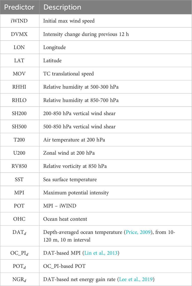
Table 1 List of atmospheric and oceanic potential predictors used to build the machine learning-based RI prediction model.

Besides NGR, this study incorporates other well-established predictors commonly employed in statistical-dynamical models for TC intensity forecasting by various organizations (DeMaria et al., 2005; Knaff et al., 2005; Kim et al., 2018). In this study, we utilized a total of 65 potential predictors, encompassing a diverse range of factors. These include 5 static predictors, 7 atmospheric synoptic predictors, SST, MPI and the POT derived from it, OHC, and 49 predictors based on the DAT. All these predictors are summarized in Table 1. To evaluate the impact of NGR on the ML-based prediction of RI events, our study uses two distinct sets of these predictors. The first set consists of commonly used predictors related to TC intensity change, as identified in numerous statistical models (in Table 1, excluding NGRs). The second set incorporates NGR into the first set in Table 1 (as illustrated in Figure 1).

Figure 1

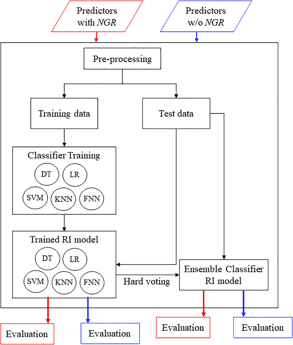
Figure 1 The flowchart of machine learning-based RI prediction model development. The dataset is divided into two parts: the training set and the testing set. The training dataset is used to build the machine learning classifiers and the testing data set is used to evaluate the performance. The ensemble classifier for RI prediction is also constructed and evaluated by using the hard-voting method.

2.3 Implementation of machine learning techniques

In this study, we employ a diverse ensemble of well-known classifiers to predict RI events in the WNP. The ensemble includes a Decision Tree (DT), Logistic Regression (LR), SVM, k-nearest Neighbors (KNN), and Feed Forward Neural Network (FNN). DT serves as a comprehensive data-mining tool, which is adept at generating decision-making rules, identifying patterns, and uncovering knowledge embedded in archived databases (Quinlan, 1987). More specifically, the DT algorithm evaluates the conduciveness of environmental conditions for RI by systematically checking whether specific environmental predictors satisfy the thresholds set by the trained tree model. LR is used to predict a categorical variable such as the class label (Walker and Duncan, 1967). It is an extension of linear regression, where the classification problem is converted into a regression problem by estimating the log (odds) of each class in place of probability itself. The model uses the logistic function to squash the output of a linear equation between 0 and 1, making it interpretable as a probability. This method is prized for its simplicity, interpretability, and effectiveness in various domains. The SVM is designed to discover a hyperplane that best separates the data classes (Cortes and Vapnik, 1995). It achieves this by maximizing the margin between different classes in the feature space. The KNN algorithm makes predictions by storing all training data and identifying the classes of the k closest neighbors to each test sample (Keller et al., 1985). It aims to classify an unknown sample based on the known classifications of its nearest neighbors. Finally, FNN is a straightforward artificial neural network composed of an input layer and an output layer. The flow of crucial input information in FNN moves strictly from its input layer to its output layer, making the model especially well-suited for parameter identification tasks (Zhang et al., 2022). Each of these classifiers brings its own set of strengths to the ensemble, contributing to a more robust and reliable RI prediction for the WNP.

To enhance predictability, we employ a hard-voting ensemble method that combines the predictions of the individual classifiers. In this approach, each classifier ‘votes’ for a class when presented with a test instance. The ensemble then selects the class that receives the majority of votes as its final prediction. By employing this hard-voting scheme, we aim to benefit from the complementary strengths of each classifier, thereby achieving a more robust and accurate model for predicting RI events in the WNP. Given that RI events are not commonly observed, as shown in Table 2, there is a clear class imbalance in our dataset. To effectively address and rectify this imbalance, we made use of the Synthetic Minority Over-sampling Technique, commonly known as SMOTE (Chawla et al., 2011). This method effectively tackles the issue of class imbalance in datasets, which is critical in many ML applications. Generating synthetic data for the minority class and creating new data points between existing ones helps balance the dataset. This balance is crucial for training unbiased models and ensuring they effectively learn the characteristics of all classes. This approach ultimately leads to an enhancement in the overall accuracy and performance of the model, making it more reliable for real-world applications. In this study, Principal Component Analysis (PCA) was applied to the pool of predictors to combat multicollinearity within the model. The integration of PCA into our ML-based classification model brought several advantages. It effectively streamlined the dataset by reducing dimensionality, which helped mitigate issues related to the curse of dimensionality and overfitting. This feature reduction also led to improved computational efficiency. Additionally, by focusing on the primary directions of data variance, PCA successfully filtered out noise and irrelevant information, resulting in a more refined dataset (Tefas and Pitas, 2016). Notably, we only used those principal components that represented at least 99% of the cumulative explained variance as predictors in our model. Given the limited size of our dataset, we employed a 10-fold cross-validation approach, ensuring the selection of the most effective models and preventing overfitting during training. The dataset from 2004 to 2018 was designated for training, while data from 2019 to 2021 was reserved for testing. Within the training data, there were 627 RI cases and 3,388 non-RI cases. Meanwhile, the testing dataset comprised 103 RI cases and 581 non-RI cases, as detailed in Table 2.

Table 2

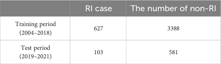
Table 2 The comparison of the number of RI and non-RI cases for training (2004–2018) and test (2019–2021) period in the western North Pacific.

2.4 Evaluating metrics

In the realm of binary classification models, the evaluation of predictor significance is pivotal for model accuracy and interpretability. Among various statistical measures, Cohen’s d is an effective tool for quantifying the discriminative power of predictors. Originally designed to measure the standardized difference between two means in psychological research, Cohen’s d can be adapted to assess how individual predictors differentiate between the two classes of the model, typically labeled positive and negative. By calculating the difference in means of a predictor for each class and dividing it by the pooled standard deviation, Cohen’s d provides a standardized effect size, facilitating direct and quantifiable comparison of the predictor’s impact across different models and datasets. Cohen’s d calculated as:

$$d=\frac{M_1-M_2}{S{D}_{pooled}}$$

where M₁ and M₂ are the means of the predictor values for each of the two classes. SD_pooledis the pooled standard deviation of the predictor values across both classed. It is computed as:

$$S{D}_{pooled}=\sqrt{\frac{(S{D}_1^2\times n_1)+(S{D}_2^2\times n_2)}{n_1+n_2-2}}$$

where SD₁ and SD₂ are the standard deviations for each class, and n₁ and n₂ are the sample sizes. A higher Cohen’s d value indicates greater separation between the classes based on the predictor, signifying its importance in the classification task. Typically, Cohen’s d values around 0.2 are considered small, around 0.5 medium, and 0.8 or higher, large. This gradation helps in pinpointing the predictors with the most significant roles in distinguishing between classes.

In binary forecasts where models predict an RI event or non-RI event for a training and test set, evaluation metrics comprise elements from a confusion matrix that compare observations to model forecasts (Table 3). True Positive (TP) is the number of correct forecasts of RI events, whereas False Positive (FP) is the number of incorrect forecasts. False Negative (FN) is the number where the model did not forecast RI but, RI was observed. True Negative (TN) is the number where the model did not forecast RI and RI was not observed.

Table 3

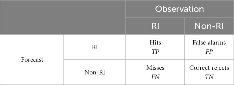
Table 3 Confusion matrix for a binary RI and non-RI classifier.

Accuracy (ACC) is used to measure the overall performance of a binary classifier and is measured as

$$ACC= \frac{TP+TN}{TP+FP+TN+FN}$$

FAR is the number of incorrect forecasts of RI divided by the total number of RI forecasts. FAR is calculated as

$$FAR=\frac{FP}{TP+FP}$$

POD) is the ratio of the correct forecasts of RI occurrences to the actual number of RI occurrences and is calculated as

$$POD=\frac{TP}{TP+FN}$$

Precision measures the accuracy of positive predictions in classification problems. It’s the ratio of the correct forecasts of RI occurrences to the total number of positive predictions (which includes both TP and FP). Precision is calculated as

$$Precision=\frac{TP}{TP+FP}$$

Peirce skill score (PSS), also known as the Hanssen-Kuipers skill score measures skill relative to an unbiased random reference forecast and is calculated as

$$PSS= \frac{(TP\times TN)-(FP\times FN)}{(TP+FN)\times (FP+TN)}$$

The F-1 score is a way of combining the precision and POD of the model, and it is defined as the harmonic mean of the model’s precision and POD. The F-1 score is calculated as

$$F-1 score=2\times \frac{POD\times Precision}{POD+Precision}$$

A perfect forecast model would achieve an ACC, POD, and PSS score of 1 and a FAR score of 0. In general, higher values of ACC, POD, Precision, PSS and F-1 score, coupled with a lower FAR, indicate superior model performance.

3 Results

3.1 Characterization of individual predictors

In this section, we examine the classification performance of potential predictors for RI events before developing a classification model. The mean distribution for RI and non-RI classes for each predictor, the effect size of the mean differences between these classes, and the correlation coefficients with the 24-hour intensity change were analyzed (Table 4; Figures 2, 3). Excluding DAT-based predictors, the ocean temperature and MPI theory-based predictors (SST, MPI, POT, OHC) exhibited the highest Cohen’s d and correlation coefficients. Following these, static predictors such as DVMX and LAT displayed the next highest values of Cohen’s d. Synoptic predictors, apart from wind shear-related predictors (SH200, SH500, U200), generally demonstrated lower predictive performance.

Table 4

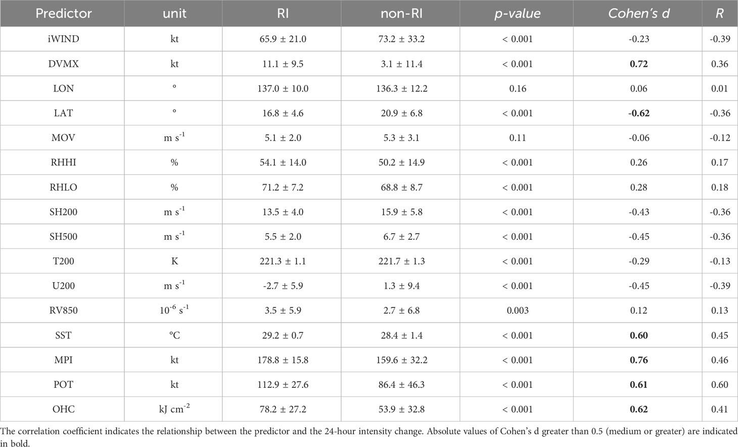
Table 4 Mean distribution of potential predictors for RI and non-RI events, p-value (student t-test) and Cohen’s d of the difference between the two groups.

Figure 2

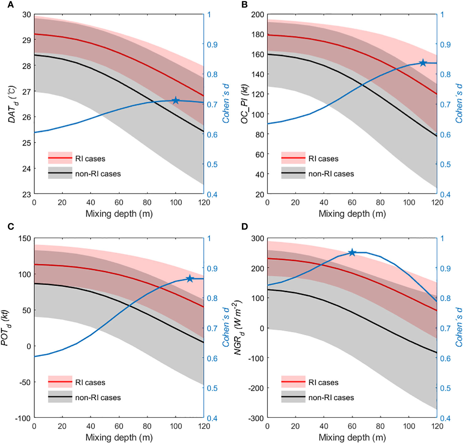
Figure 2 The comparison of the mean distribution of each class for (A) DAT_d, (B) OC_PI_d, (C) POT_d and (D) NGRd. The predictors are based on the computed average ocean temperature from the surface down to a depth of 120 meters (in 10-meter intervals) over the period 2004–2021. The red (black) solid line and shade indicate the mean value and ±1 σ range of RI (non-RI) class, respectively. Cohen’s d values (blue line) show the effect size of mean differences between RI and non-RI classes.

Figure 3

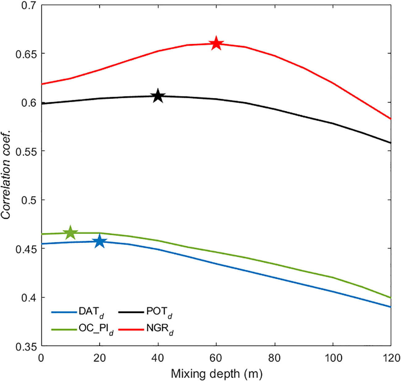
Figure 3 The comparison of the correlation coefficients between depth-averaged temperature-based predictors and 24-hour intensity change. The predictors are based on the computed average ocean temperature from the surface down to a depth of 120 meters (in 10-meter intervals) over the period 2004–2021. Pentagrams represent the location of the maximum correlation coefficient for each group.

DAT-based predictors demonstrated higher Cohen’s d values compared to those derived from traditional SST (Figure 2). For DAT-based predictors, excluding NGR_d, Cohen’s d between the two classes increased progressively with greater mixing depths, peaking at depths of 100-110 meters. NGR_d, in contrast, displayed a steadily increasing Cohen’s d value with depth, reaching a peak at 60 meters and demonstrating a higher Cohen’s d value that overshadowed the other potential predictors. Figure 3 illustrates distinct patterns of correlation for each predictor as a function of mixing depth, indicating that the relationship between predictors and TC intensity change is sensitive to the mixing depth. Notably, NGR_d emerges as a superior predictor, with its maximum correlation coefficient occurring at a mixing depth of 60 meters (Figure 3, red line). This is not only higher than those of other predictors but also aligns with the depth where Cohen’s d—a statistical measure of effect size—reaches its peak (Figure 2D, blue line). The consistency of the NGR_d peak with the maximum of Cohen’s d at 60 meters suggests a strong and possibly causal relationship between DATs of this depth and TC intensification rates, as well as RI events. This underscores the value of NGR_d, based on 60-meter DAT, as a potentially powerful single predictor for anticipating changes in TC intensity, which is crucial for early warning systems and preparedness measures in vulnerable coastal regions.

3.2 Assessment of model predictive performance

As outlined in Figure 4 and Table 5, our study includes a comprehensive summary of the performance metrics — POD, PSS, FAR, Precision, ACC, and F-1 score — for individual ML models. These were evaluated during the training period running from 2014 to 2018. A modest change emerged when we incorporated NGRs into the predictor pools: the metrics of POD, Precision, PSS, F-1 score and ACC generally increased across the models, while the FAR metric correspondingly decreased. The only exception to this was observed in the DT model. This underscores the relevance and value of incorporating NGRs into the feature set, as models with NGRs consistently outperformed those without. Individually, the NGR-based FNN exhibited the highest predictive performance overall, closely followed by the SVM model.

Figure 4

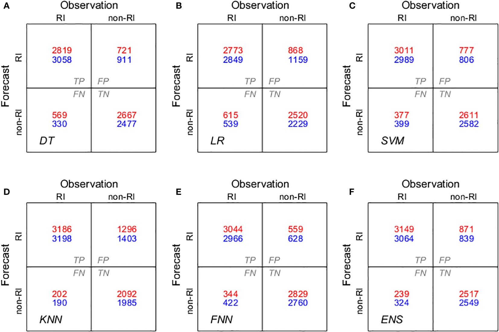
Figure 4 Binary confusion metrics of the developed models during the training period: (A) DT, (B) LR, (C) SVM, (D) KNN, (E) FNN, and (F) hard voting ensemble (ENS) of the above models. The red indicates the NGR-based model’s outcomes, while the blue shows the performance of the non-NGR model.

Table 5

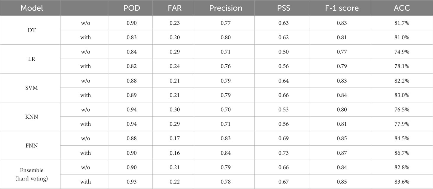
Table 5 Performance metrics for the individual model and ensemble with NGR-based predictors and without NGR-based predictors for the training period (2014–2018).

During the test period of 2019 to 2021, summarized in Figure 5 and Table 6, the favorable impact of NGRs was further corroborated. NGRs-based models once again outperformed their counterparts that lacked this feature. This improvement is related to the increase in the number of samples in TN. NGR-based models detected non-RI cases relatively better (Figure 5). Among the individual models, the NGR-based SVM emerged as the best performer, particularly in terms of PSS. The consistency of this impact across both training and test periods reaffirms the generalizability and reliability of our methodological approach. An interesting point of divergence between the training and test periods was in the performance indicators. In addressing the class imbalance, oversampling was applied during the training phase. However, this method artificially inflates the TP count. The notable increase in POD and a corresponding decrease in FAR during the training period is attributable to the oversampling technique employed. Because oversampling is not performed in the testing phase, the ratio of RI cases decreases significantly compared to the training phase. This results in a relatively large decrease in TP, which in turn inflates FAR. This highlights the distortion in model performance metrics due to the uneven application of oversampling across training and testing datasets.

Figure 5

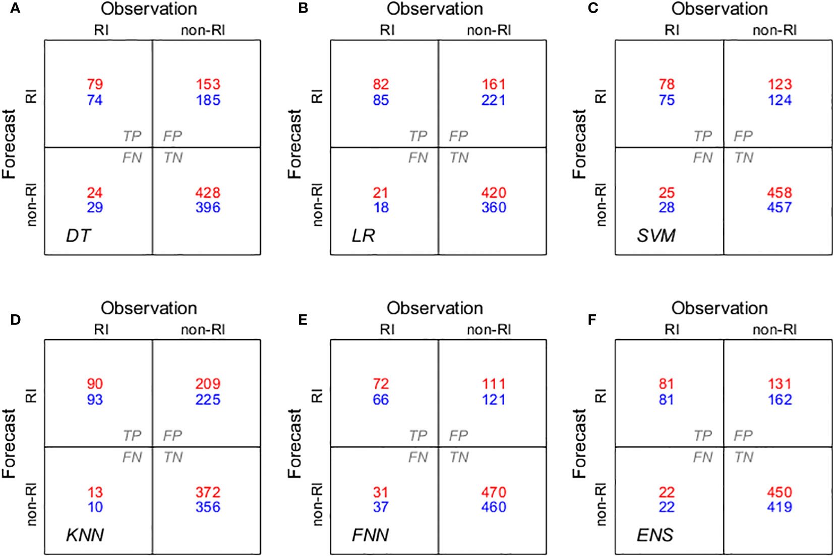
Figure 5 Same as Figure 4, but for test period.

Table 6

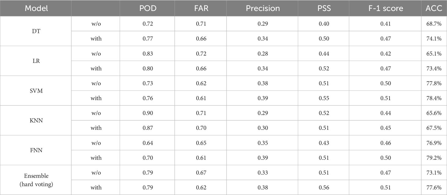
Table 6 Same as Table 5, but for the test period (2019–2021).

To generate an ensemble forecast, we employ a hard-voting method based on the collective performance metrics of five distinct classifiers. Our ensemble performance metrics for the training and test are shown in Table 5 and Table 6, respectively. What becomes evident is that integrating NGRs into our ensemble model substantially augments its predictive capabilities. This improvement is noticeable during the test period. Notably, the PSS and F-1 score saw a 10% increase when NGRs were included in the ensemble model, demonstrating a more skillful forecast (Table 6).

To contextualize our ensemble’s performance, it is useful to compare it with other contemporary ML-based RI forecasting models. Wei et al. (2023) presented a deep learning network model called TCNET, which they compared against two Statistical Hurricane Intensity Prediction Schemes (SHIPS)-based models (COR-SHIPS and LLE-SHIPS), along with other models from Yang (2016); henceforth referred to as Y16) and Kaplan et al. (2015); henceforth referred to as KRD15). Ko et al. (2023) explored the application of a consensus machine learning (CML) model in TC intensity change forecasting and indicated the CML exhibits better performance on RI predictions compared to the operational models such as SHIPS, GFS. Narayanan et al. (2023) proposed a simple deterministic binary classification model based on the co-occurrence of environmental parameters (MCE) to predict an RI event. Their results indicated that MCE shows improved skill over the decision tree and logistic regression models, with more accurate RI predictions in the overall testing dataset. The PSS values for these models, displayed in Figure 6, show that our ensemble model (NGR-ENS), with a PSS of 0.56 and a POD of 0.79, surpasses all these competing models including TCNET (0.48), MCE (0.40) and CML (0.50). TCNET has the lowest FAR (0.43) followed by CML (0.50), LLE-SHIPS (0.56) and NGR-ENS (0.62). This holds even when considering different target periods or datasets. In essence, our ensemble approach fortified by the inclusion of NGRs offers superior predictive accuracy for RI events with an advantage of the noticeably high POD rate and the relatively low FAR rate.

Figure 6

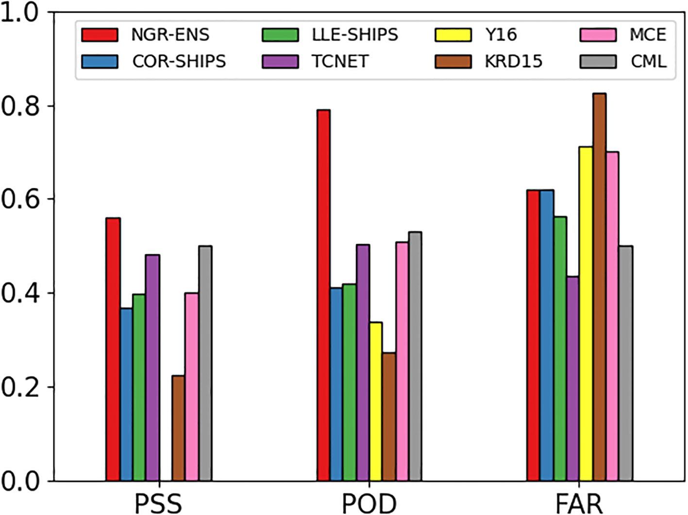
Figure 6 Performance metric values for the COR-SHIPS (blue), LLE-SHIPS (green), TCNET (purple), Y16 (yellow), KRD15 (brown), MCE (pink), CML (gray) models and the comparisons of NGR-ENS (red) model developed in this study.

Lee et al. (2016) suggested that the bimodal distribution of lifetime maximum intensity in TCs can be attributed to two distinct types of TC: those that experience RI (RI storms) and those that do not (non-RI storms). They showed that a significant majority—79%—of major TCs, those classified as category 3 or above, belong to the RI storm. Conversely, only a small fraction—6%—of non-RI storms ever escalate to become major TCs. Therefore, RI prediction performance in major TCs can represent the overall prediction performance. During the test period (2019 –2021), our ensemble model showed noticeable performance improvements when NGR was included as a variable (Table 7). A recent C_d parameterization study showed that C_d decreases after saturating at 33 m s^-1, which leads to an increase in NGR, which can induce RI (Kim et al., 2022). These findings suggest that accurately simulating flux exchanges, especially in storms ranging from categories 1–3, can substantially enhance the model’s ability to predict RI accurately.

Table 7

Table 7 Performance metrics for the ensemble of five prediction models for major TCs during the test period (2019–2021).

4 Conclusions and discussions

In this study, the binary RI prediction model by incorporating the NGR which was derived using the upper ocean thermal structure of pre-storm ocean and a realistic parameterization of sea surface roughness, into the ML models have been developed for the WNP. Five ML experiments were conducted to predict RI classification predictions, using five ML techniques- DT, LR, SVM, KNN, and FNN-trained with widely used predictors. To investigate the impact of NGR on RI prediction, two sets of experiments were conducted for each ML model. In the first set, models were trained only with well-known existing predictors, while in the second set, NGR was also included. For the training period, compared with the traditional predictors, the results with the newly used predictors, NGRs, in this study show improved skill over all the ML models except for DT. For the test period, all the ML models trained with NGRs are, again, better performance with higher POD, PSS, ACC, and lower FAR than the same model but trained without NGRs. An ensemble average of the individual five ML models is constructed based on the hard-voting method. We show that the ensemble ML model produces noteworthy improvements for RI in the WNP. The inclusion of the NGRs input from the predictor pool in the ensemble model enhances RI prediction performance (PSS) by approximately 10% compared to the ensemble model without NGRs. These results suggest that the inclusion of NGR contributes to more accurate statistical-dynamical predictions of RI, corroborating previous findings that the NGR index better estimates changes in TC intensity in the WNP (LEE19).

In our study, we employed PCA to tackle the challenges associated with a high-dimensional dataset, particularly the risk of overfitting. Overfitting could jeopardize both the model’s reliability and its ability to generalize to new data. PCA ameliorated this by compressing the data dimensions while retaining the most important variance, thereby enhancing the model’s reliability. In this study, we checked the performance of the prediction model with and without PCA to confirm the improvement in prediction performance through PCA. During the training period, the application of PCA did not significantly impact the predictive performance of the model. However, during the test period, the model that applied PCA showed approximately 10% higher prediction performance than the model that did not apply it (based on NGR-ENS). Using PCA to reduce model overfitting effectively reduces dimensions while retaining key information and eliminating unnecessary noise. This approach prevents the model from being overly optimized for training data, enhancing its generalization ability. PCA lowers the risk of overfitting seen in high-dimensional data when considering all features, which can lead to better performance on both training and testing data. Thus, PCA plays a crucial role in decreasing model complexity and improving predictive capabilities by capturing essential patterns and structures. However, it is worth noting that PCA comes with limitations, such as reduced interpretability due to the transformation of original variables into principal components. This makes it difficult to make intuitive sense of the model’s features. Additionally, PCA may overlook non-linear relationships between variables, potentially missing out on important data patterns. Despite these drawbacks, the computational efficiency and reduced risk of overfitting achieved through PCA were indispensable for improving our model’s overall reliability and stability.

This study focused on the WNP. To ascertain the broader applicability of these models, they should be trialed in different basins. It is pivotal to understand if the NGR-based approach’s efficacy remains consistent irrespective of region. The current study employs a 10-m intervals depth-based DAT in NGR calculations. A more adaptive approach might involve modulating the depth contingent on real-time TC characteristics like its intensity, speed, latitude, and size. Such dynamism can potentially enhance the precision of the NGR, leading to improved predictions. Apart from NGR, there might be other indices or predictors that can be tested alongside or against the NGR to see which provides the most accurate results. This could lead to a more robust model or a combination of indices for improved RI prediction. The choice of the hard-voting ensemble method was predominantly due to SVM’s characteristics. Yet, diversifying into other ensemble strategies, including weighted voting or stacking, may offer a finer prediction approach.

Understanding time series data often unveils serial dependence, where each data point is potentially influenced by its predecessors. This temporal dependency implies that past observations significantly impact present and future values (Box and Pierce, 1970; Ljung and Box, 1978). Similarly, in spatial data, we observe a spatial dependency, where the characteristics of a specific location may be influenced by its neighboring areas. Traditional ML models typically struggle with these dependencies. They often assume that data points are independent and identically distributed, an assumption that falls short in the context of time series and spatial data. To better handle these types of data, it’s crucial to integrate information about past values in the case of time series (lagged values) and details about neighboring locations in spatial data into the models. This enrichment of the feature set allows the models to acknowledge and utilize these dependencies, enhancing their effectiveness. While advanced deep learning methods, like CNNs and Recurrent Neural Networks (RNNs), provide comprehensive solutions for handling these complexities, simpler adaptations to existing methodologies can also be effective and offer more interpretability. The future of research in this area lies in exploring these strategies to improve the capabilities of models, making them more accurate and reliable in mirroring the dynamics of time series and spatial data. This improvement is particularly relevant for robust and accurate prediction in real-world applications, such as RI prediction. By focusing on these aspects, significant advancements in the robustness and accuracy of RI prediction models are anticipated, enhancing their applicability in practical scenarios.

Data availability statement

TC data can be found on the IBTrACS website (https://www.ncei.noaa.gov/data/international-best-track-archive-for-climate-stewardship-ibtracs/v04r00/access/netcdf/), GFS 6-hourly data at https://www.ncei.noaa.gov/data/global-forecast-system/access/, HYCOM+NCODA data at https://www.hycom.org/dataserver/gofs-3pt1/analysis.

Author contributions

S-HK: Conceptualization, Data curation, Formal analysis, Methodology, Writing – original draft, Writing – review & editing. WL: Conceptualization, Formal analysis, Methodology, Validation, Writing – review & editing. H-WK: Formal analysis, Supervision, Validation, Writing – review & editing. SK: Supervision, Validation, Writing – review & editing.

Funding

The author(s) declare financial support was received for the research, authorship, and/or publication of this article. This research was a part of the project titled “Study on Northwestern Pacific warming and genesis and rapid intensification of typhoon”, funded by the Ministry of Oceans and Fisheries, Korea (20220566). This work was also funded by the Korea Meteorological Administration Research and Development Program “Development of Asian Dust and Haze Monitoring and Prediction Technology” under Grant (KMA2018-00521).

Conflict of interest

The authors declare that the research was conducted in the absence of any commercial or financial relationships that could be construed as a potential conflict of interest.

Publisher’s note

All claims expressed in this article are solely those of the authors and do not necessarily represent those of their affiliated organizations, or those of the publisher, the editors and the reviewers. Any product that may be evaluated in this article, or claim that may be made by its manufacturer, is not guaranteed or endorsed by the publisher.

Supplementary material

The Supplementary Material for this article can be found online at: https://www.frontiersin.org/articles/10.3389/fmars.2023.1296274/full#supplementary-material

References

Balaguru K., Foltz G. R., Leung L. R. (2018). Increasing magnitude of hurricane rapid intensification in the central and eastern tropical Atlantic. Geophys. Res. Lett. 45 (9), 4238–4247. doi: 10.1029/2018GL077597

CrossRef Full Text | Google Scholar

Bender M. A., Ginis I., Tuleya R., Thomas B., Marchok T. (2007). The operational GFDL coupled hurricane–ocean prediction system and a summary of its performance. Monthly Weather Rev. 135 (12), 3965–3989. doi: 10.1175/2007MWR2032.1

CrossRef Full Text | Google Scholar

Biswas M. K., Abarca S., Bernardet L., Ginis I., Grell E., Iacono M., et al. (2018). Hurricane weather research and forecasting (HWRF) Model: 2017 scientific Documentation (Technical Report) (Boulder, CO: National Center for Atmospheric Research and Developmental Testbed Center).

Google Scholar

Box G. E. P., Pierce D. A. (1970). Distribution of residual autocorrelations in autoregressive-integrated moving average time series models. J. Am. Statist. Assoc. 65, 1509–1526. doi: 10.1080/01621459.1970.10481180

CrossRef Full Text | Google Scholar

Chawla N. V., Bowyer K. W., Hall L. O., Kegelmeyer W. P. (2011). SMOTE: Synthetic minority over-sampling technique. J. Artif. Intell. Res. 16, 321–357. doi: 10.1613/jair.953

CrossRef Full Text | Google Scholar

Chen X., Bryan G. H., Hazelton A., Marks F. D., Fitzpatrick P. (2022). Evaluation and improvement of a TKE-based eddy-diffusivity mass-flux (EDMF) planetary boundary layer scheme in hurricane conditions. Weather Forecast. 37 (6), 935–951. doi: 10.1175/WAF-D-21-0168.1

CrossRef Full Text | Google Scholar

Cloud K. A., Reich B. J., Rozoff C. M., Alessandrini S., Lewis W. E., Delle Monache L. (2019). A feed forward neural network based on model output statistics for short-term hurricane intensity prediction. Weather Forecasting 34 (4), 985–997. doi: 10.1175/WAF-D-18-0173.1

CrossRef Full Text | Google Scholar

Cortes C., Vapnik V. (1995). Support-vector networks. Mach. Learn (20), 273–297. doi: 10.1007/BF00994018

CrossRef Full Text | Google Scholar

DeMaria M., Franklin J. L., Onderlinde M. J., Kaplan J. (2021). Operational forecasting of tropical cyclone rapid intensification at the National Hurricane Center. Atmosphere 12 (6), 683. doi: 10.3390/atmos12060683

CrossRef Full Text | Google Scholar

DeMaria M., Kaplan J. (1994). Sea surface temperature and the maximum intensity of Atlantic tropical cyclones. J. Climate 7 (9), 1324–1334. doi: 10.1175/1520-0442(1994)007<1324:SSTATM>2.0.CO;2

CrossRef Full Text | Google Scholar

DeMaria M., Kaplan J. (1999). An updated statistical hurricane intensity prediction scheme (SHIPS) for the Atlantic and eastern North Pacific basins. Weather Forecasting 14 (3), 326–337. doi: 10.1175/1520-0434(1999)014<0326:AUSHIP>2.0.CO;2

CrossRef Full Text | Google Scholar

DeMaria M., Mainelli M., Shay L. K., Knaff J. A., Kaplan J. (2005). Further improvements to the statistical hurricane intensity prediction scheme (SHIPS). Weather Forecast. 20 (4), 531–543. doi: 10.1175/WAF862.1

CrossRef Full Text | Google Scholar

Emanuel K. A. (1986). An air-sea interaction theory for tropical cyclones. Part I: Steady-state maintenance. J. Atmospheric Sci. 43 (6), 585–605. doi: 10.1175/1520-0469(1986)043<0585:AASITF>2.0.CO;2

CrossRef Full Text | Google Scholar

Emanuel K. A. (1988). The maximum intensity of hurricanes. J. Atmos. Sci. 45 (7), 1143–1155. doi: 10.1175/1520-0469(1988)045<1143:TMIOH>2.0.CO;2

CrossRef Full Text | Google Scholar

Emanuel K. A. (1995). Sensitivity of tropical cyclones to surface exchange coefficients and a revised steady-state model incorporating eye dynamics. J. Atmospheric Sci. 52 (22), 3969–3976. doi: 10.1175/1520-0469(1995)052<3969:SOTCTS>2.0.CO;2

CrossRef Full Text | Google Scholar

Feng J., Wang X. (2021). Impact of increasing horizontal and vertical resolution during the HWRF hybrid En Var data assimilation on the analysis and prediction of Hurricane Patricia, (2015). Monthly Weather Rev. 149, 419–441. doi: 10.1175/MWR-D-20-0144.1

CrossRef Full Text | Google Scholar

Gao S., Zhang W., Liu J., Lin I. I., Chiu L. S., Cao K. (2016). Improvements in typhoon intensity change classification by incorporating an ocean coupling potential intensity index into decision trees. Weather Forecasting 31 (1), 95–106. doi: 10.1175/WAF-D-15-0062.1

CrossRef Full Text | Google Scholar

Goldenberg S. B., Gopalakrishnan S. G., Tallapragada V., Quirino T., Marks F. Jr., Trahan S., et al. (2015). The 2012 triply nested, high-resolution operational version of the Hurricane Weather Research and Forecasting Model (HWRF): Track and intensity forecast verifications. Weather Forecasting 30 (3), 710–729. doi: 10.1175/WAF-D-14-00098.1

CrossRef Full Text | Google Scholar

Griffin S. M., Wimmers A., Velden C. S. (2022). Predicting rapid intensification in North Atlantic and eastern North Pacific tropical cyclones using a convolutional neural network. Weather Forecasting 37 (8), 1333–1355. doi: 10.1175/WAF-D-21-0194.1

CrossRef Full Text | Google Scholar

Kaplan J., DeMaria M. (2003). Large-scale characteristics of rapidly intensifying tropical cyclones in the North Atlantic basin. Weather forecasting 18 (6), 1093–1108. doi: 10.1175/1520-0434(2003)018<1093:LCORIT>2.0.CO;2

CrossRef Full Text | Google Scholar

Kaplan J., DeMaria M., Knaff J. A. (2010). A revised tropical cyclone rapid intensification index for the Atlantic and Eastern North Pacific Basins. Weather Forecast. 25 (1), 220–241. doi: 10.1175/2009WAF2222280.1

CrossRef Full Text | Google Scholar

Kaplan J., Rozoff C. M., DeMaria M., Sampson C. R., Kossin J. P., Velden C. S., et al. (2015). Evaluating environmental impacts on tropical cyclone rapid intensification predictability utilizing statistical models. Weather Forecasting 30 (5), 1374–1396. doi: 10.1175/WAF-D-15-0032.1

CrossRef Full Text | Google Scholar

Keller J. M., Gray M. R., Givens J. A. (1985). A fuzzy k-nearest neighbor algorithm. IEEE Trans. systems man cybernetics 4), 580–585. doi: 10.1109/TSMC.1985.6313426

CrossRef Full Text | Google Scholar

Kim H. J., Moon I. J., Oh I. (2022). Comparison of tropical cyclone wind radius estimates between the KMA, RSMC tokyo, and JTWC. Asia-Pac J. Atmos Sci. 58, 563–576. doi: 10.1007/s13143-022-00274-5

CrossRef Full Text | Google Scholar

Kim S. H., Kang H. W., Moon I. J., Kang S. K., Chu P. S. (2022). Effects of the reduced air-sea drag coefficient in high winds on the rapid intensification of tropical cyclones and bimodality of the lifetime maximum intensity. Front. Mar. Sci. 9. doi: 10.3389/fmars.2022.1032888

PubMed Abstract | CrossRef Full Text | Google Scholar

Kim S. H., Moon I. J., Chu P. S. (2018). Statistical–dynamical typhoon intensity predictions in the Western North Pacific using track pattern clustering and ocean coupling predictors. Weather Forecasting 33 (1), 347–365. doi: 10.1175/WAF-D-17-0082.1

CrossRef Full Text | Google Scholar

Klotzbach P. J., Wood K. M., Schreck C. J. III, Bowen S. G., Patricola C. M., Bell M. M. (2022). Trends in global tropical cyclone activity: 1990–2021. Geophys. Res. Lett. 49 (6), e2021GL095774. doi: 10.1029/2021GL095774

CrossRef Full Text | Google Scholar

Knaff J. A., Sampson C. R., DeMaria M. (2005). An operational statistical typhoon intensity prediction scheme for the western North Pacific. Weather Forecasting 20 (4), 688–699. doi: 10.1175/WAF863.1

CrossRef Full Text | Google Scholar

Knutson T., Camargo S. J., Chan J. C., Emanuel K., Ho C. H., Kossin J., et al. (2020). Tropical cyclones and climate change assessment: Part II: Projected response to anthropogenic warming. Bull. Am. Meteorol. Soc. 101 (3), E303–E322. doi: 10.1175/BAMS-D-18-0194.1

CrossRef Full Text | Google Scholar

Ko M. C., Chen X., Kubat M., Copalakrishnan S. (2023). The Development of a consensus machine learning model for hurricane rapid intensification forecasts with hurricane weather research and forecasting (HWRF) data. Weather Forecasting 38, 1253–1270. doi: 10.1175/WAF-D-22-0217.1

CrossRef Full Text | Google Scholar

Kossin J. P., Knapp K. R., Olander T. L., Velden C. S. (2020). Global increase in major tropical cyclone exceedance probability over the past four decades. Proc. Natl. Acad. Sci. 117 (22), 11975–11980. doi: 10.1073/pnas.1920849117

CrossRef Full Text | Google Scholar

Lee W., Kim S. H., Chu P. S., Moon I. J., Soloviev A. V. (2019). An index to better estimate tropical cyclone intensity change in the western North Pacific. Geophys. Res. Lett. 46 (15), 8960–8968. doi: 10.1029/2019GL083273

CrossRef Full Text | Google Scholar

Lee W., Kim S. H., Moon I.-J., Bell M. M., Ginis I. (2022). New parameterization of air-sea exchange coefficients and its impact on intensity prediction under major tropical cyclones. Front. Mar. Sci. 9. doi: 10.3389/fmars.2022.1046511

PubMed Abstract | CrossRef Full Text | Google Scholar

Lee C. Y., Tippett M. K., Sobel A. H., Camargo S. J. (2016). Rapid intensification and the bimodal distribution of tropical cyclone intensity. Nat. Commun. 7, 10625. doi: 10.1038/ncomms10625

PubMed Abstract | CrossRef Full Text | Google Scholar

Li J., Wan Q., Xu D., Huang Y., Zhang X. (2021). An initialization scheme for weak tropical cyclones in the south China sea. J. Meteorol. Res. 35, 358–370. doi: 10.1007/s13351-021-0069-3

CrossRef Full Text | Google Scholar

Li Q., Li Z., Peng Y., Wang X., Li L., Lan H., et al. (2018). Statistical regression scheme for intensity prediction of tropical cyclones in the Northwestern Pacific. Weather Forecasting 33, 1299–1315. doi: 10.1175/WAF-D-18-0001.1

CrossRef Full Text | Google Scholar

Lin I. I., Black P., Price J. F., Yang C. Y., Chen S. S., Lien C. C., et al. (2013). An ocean coupling potential intensity index for tropical cyclones. Geophys. Res. Lett. 40 (9), 1878–1882. doi: 10.1002/grl.50091

CrossRef Full Text | Google Scholar

Liu Q., Zhang X., Tong M., Zhang Z., Liu B., Wang W., et al. (2020). Vortex initialization in the NCEP operational hurricane models. Atmosphere 11, 968. doi: 10.3390/atmos11090968

CrossRef Full Text | Google Scholar

Ljung G., Box G. C. (1978). On a measure of lack of fit in time series models. Biometrica 65, 265–270. doi: 10.1093/biomet/65.2.297

CrossRef Full Text | Google Scholar

Lu X., Davis B., Wang X. (2022). Improving the Assimilation of enhanced atmospheric motion vectors for hurricane intensity predictions with HWRF. Remote Sens. 14, 2040. doi: 10.3390/rs14092040

CrossRef Full Text | Google Scholar

Magnusson L., Majumdar S., Emerton R., Richardson D., Alonso-Balmaseda M., Baugh C., et al. (2021). ECMWF Technical Memorandum No. 888 (European Centre for Medium-Range Weather Forecasts). doi: 10.21957/zzxzzygwv

CrossRef Full Text | Google Scholar

Mercer A., Grimes A. (2017). Atlantic tropical cyclone rapid intensification probabilistic forecasts from an ensemble of machine learning methods. Proc. Comput. Sci. 114, 333–340. doi: 10.1016/j.procs.2017.09.036

CrossRef Full Text | Google Scholar

Murakami H., Wang B., Li T., Kitoh A. (2013). Projected increase in tropical cyclones near Hawaii. Nat. Climate Change 3 (8), 749–754. doi: 10.1038/nclimate1890

CrossRef Full Text | Google Scholar

Narayanan A., Balaguru K., Xu W., Leung L. R. (2023). A new method for predicting hurricane rapid intensification based on co-occurring environmental parameters. Nat. Hazards. doi: 10.1007/s11069-023-06100-z

CrossRef Full Text | Google Scholar

Ooyama K. (1969). Numerical simulation of the life cycle of tropical cyclones. J. Atmospheric Sci. 26 (1), 3–40. doi: 10.1175/1520-0469(1969)026<0003:NSOTLC>2.0.CO;2

CrossRef Full Text | Google Scholar

Price J. F. (2009). Metrics of hurricane-ocean interaction: vertically-integrated or vertically-averaged ocean temperature? Ocean Sci. 5 (3), 351–368. doi: 10.5194/os-5-351-2009

CrossRef Full Text | Google Scholar

Quinlan J. R. (1987). Simplifying decision trees. Int. J. man-machine Stud. 27 (3), 221–234. doi: 10.1016/S0020-7373(87)80053-6

CrossRef Full Text | Google Scholar

Rozoff C. M., Kossin J. P. (2011). New probabilistic forecast models for the prediction of tropical cyclone rapid intensification. Weather Forecasting 26 (5), 677–689. doi: 10.1175/WAF-D-10-05059.1

CrossRef Full Text | Google Scholar

Shaiba H., Hahsler M. (2016). Applying machine learning methods for predicting tropical cyclone rapid intensification events. Res. J. Appl. Sciences Eng. Technol. 13 (8), 638–651. doi: 10.19026/rjaset.13.3050

CrossRef Full Text | Google Scholar

Soloviev A. V., Lukas R., Donelan M. A., Haus B. K., Ginis I. (2014). The air-sea interface and surface stress under tropical cyclones. Sci. Rep. 4, 5306. doi: 10.1038/srep05306

PubMed Abstract | CrossRef Full Text | Google Scholar

Song X., Zhu Y., Peng J., Guan H. (2018). Improving multi-model ensemble forecasts of tropical cyclone intensity using Bayesian model averaging. J. Meteorol. Res. 32 (5), 794–803. doi: 10.1007/s13351-018-7117-7

CrossRef Full Text | Google Scholar

Su H., Wu L., Jiang J. H., Pai R., Liu A., Zhai A. J., et al. (2020). Applying satellite observations of tropical cyclone internal structures to rapid intensification forecast with machine learning. Geophys. Res. Lett. 47 (17), e2020GL089102. doi: 10.1029/2020GL089102

CrossRef Full Text | Google Scholar

Tefas A., Pitas I. (2016). Principal component analysis. Intelligent Syst. 487.

Google Scholar

Walker S. H., Duncan D. B. (1967). Estimation of the probability of an event as a function of several independent variables. Biometrika 54 (1), 167–179.

PubMed Abstract | Google Scholar

Wang S., Toumi R. (2021). Recent tropical cyclone changes inferred from ocean surface temperature cold wakes. Sci. Rep. 11, 22269. doi: 10.1038/s41598-021-01612-9

PubMed Abstract | CrossRef Full Text | Google Scholar

Wang W., Liu B., Zhang Z., Mehra A., Tallapragada V. (2022). Improving low-level wind simulations of tropical cyclones by a regional Hurricane Analysis and Forecast System. Res. Activities Earth Syst. Model. Working Group on Numerical Experimentation, WMO, Geneva, pp. 9–10.

Google Scholar

Wei Y., Yang R., Sun D. (2023). Investigating tropical cyclone rapid intensification with an advanced artificial intelligence system and gridded reanalysis data. Atmosphere 14 (2), 195. doi: 10.3390/atmos14020195

CrossRef Full Text | Google Scholar

Xu W., Balaguru K., August A., Lalo N., Hodas N., DeMaria M., et al. (2021). Deep learning experiments for tropical cyclone intensity forecasts. Weather Forecasting 36 (4), 1453–1470. doi: 10.1175/WAF-D-20-0104.1

CrossRef Full Text | Google Scholar

Yamaguchi M., Owada H., Shimada U., Sawada M., Iriguchi T., Musgrave K. D., et al. (2018). Tropical cyclone intensity prediction in the western North Pacific basin using SHIPS and JMA/GSM. SOLA 14, 138–143. doi: 10.2151/sola.2018-024

CrossRef Full Text | Google Scholar

Yang R. (2016). A systematic classification investigation of rapid intensification of atlantic tropical cyclones with the SHIPS database. Weather Forecasting 31 (2), 495–513. doi: 10.1175/WAF-D-15-0029.1

CrossRef Full Text | Google Scholar

Zhang Y., Zhang Y., Zhou X. (2022). Classification of power quality disturbances using visual attention mechanism and feed-forward neural network. Measurement 188, 110390. doi: 10.1016/j.measurement.2021.110390

CrossRef Full Text | Google Scholar

Zhang Z., Tong M., Sippel J. A., Mehra A., Zhang B., Wu K. (2020). The impact of stochastic physics-based hybrid GSI/EnKF data assimilation on hurricane forecasts using EMC operation hurricane modeling system. Atmosphere 11, 801. doi: 10.3390/atmos11080801

CrossRef Full Text | Google Scholar

Zhang Z., Wang W., Doyle J. J., Maskaitis J., Komaromi W. A., Heming J., et al. (2023). A review of recent advances, (2018-2021) on tropical cyclone intensity change from operational perspectives, Part 1: Dynamical model guidance. Trop. Cyclone Res. Rev. 12 (1), 30–49. doi: 10.1016/j.tcrr.2023.05.004

CrossRef Full Text | Google Scholar