 Hunter P. Hughes
 Donna Surge
 Ian J. Orland
 Michael L. Zettler
 David K. Moss
- 1Earth, Marine and Environmental Sciences, University of North Carolina, Chapel Hill, NC, United States
- 2Department of Geoscience, University of Wisconsin-Madison, Madison, WI, United States
- 3Wisconsin Geological and Natural History Survey, University of Wisconsin-Madison, Madison, WI, United States
- 4Department of Biological Oceanography, Leibniz-Institute for Baltic Sea Research, Rostock, Germany
- 5Sam Houston State University, Environmental and Geosciences, Huntsville, TX, United States
Introduction: Astarte borealis holds great potential as an archive of seasonal paleoclimate, especially due to its long lifespan (several decades to more than a century) and ubiquitous distribution across high northern latitudes. Furthermore, recent work demonstrates that the isotope geochemistry of the aragonite shell is a faithful proxy of environmental conditions. However, the exceedingly slow growth rates of A. borealis in some locations (<0.2mm/year) make it difficult to achieve seasonal resolution using standard micromilling techniques for conventional stable isotope analysis. Moreover, oxygen isotope (δ18O) records from species inhabiting brackish environments are notoriously difficult to use as paleoclimate archives because of the simultaneous variation in temperature and δ18Owater values.
Methods: Here we use secondary ion mass spectrometry (SIMS) to microsample an A. borealis specimen from the southern Baltic Sea, yielding 451 SIMS δ18Oshell values at sub-monthly resolution.
Results: SIMS δ18Oshell values exhibit a quasi-sinusoidal pattern with 24 local maxima and minima coinciding with 24 annual growth increments between March 1977 and the month before specimen collection in May 2001.
Discussion: Age-modeled SIMS δ18Oshell values correlate significantly with both in situ temperature measured from shipborne CTD casts (r2 = 0.52, p<0.001) and sea surface temperature from the ORAS5-SST global reanalysis product for the Baltic Sea region (r2 = 0.42, p<0.001). We observe the strongest correlation between SIMS δ18Oshell values and salinity when both datasets are run through a 36-month LOWESS function (r2 = 0.71, p < 0.001). Similarly, we find that LOWESS-smoothed SIMS δ18Oshell values exhibit a moderate correlation with the LOWESS-smoothed North Atlantic Oscillation (NAO) Index (r2 = 0.46, p<0.001). Change point analysis supports that SIMS δ18Oshell values capture a well-documented regime shift in the NAO circa 1989. We hypothesize that the correlation between the SIMS δ18Oshell time series and the NAO is enhanced by the latter’s influence on the regional covariance of water temperature and δ18Owater values on interannual and longer timescales in the Baltic Sea. These results showcase the potential for SIMS δ18Oshell values in A. borealis shells to provide robust paleoclimate information regarding hydroclimate variability from seasonal to decadal timescales.
1 Introduction
Over the last 30 years and starting with the work of Dettman and Lohmann (1993); Dettman and Lohmann (1995), innovations in microsampling techniques for stable isotope analysis of freshwater to marine organisms with accretionary carbonate hard parts (e.g., bivalves, gastropods, corals, and fish) have spurred discoveries in fields such as paleoclimatology, paleobiology, and archaeology (special issues Schöne and Surge, 2005; Prendergast et al., 2017 and references therein). The ability to microsample some archives at seasonal-scale resolution gave rise to the broader field of isotope sclerochronology, which combines the use of growth patterns with oxygen and stable carbon isotope ratios (δ18O and δ13C, respectively) recorded in carbonate hard parts (Schöne and Surge, 2012; Surge and Schöne, 2015). In bivalves, shell growth patterns (growth lines and increments) are formed due to changes in the rate of carbonate deposition that is, in turn, a response to environmental and biological conditions at several periodicities: daily, tidal, fortnightly, monthly, and annual (Barker, 1964; Stanley, 1966; Pannella and MacClintock, 1968; Clark, 1974; Pannella, 1976; Jones et al., 1983; Goodwin et al., 2001). In effect, growth increments form a shell calendar that can be used to measure time. When combined with shell oxygen isotope (δ18O) ratios, which are a function of growth temperature and δ18O values of ambient water, shell calendars are rich bioarchives of past environments and climate conditions.
The vast majority of studies using high-resolution, seasonal-scale records from fast- and slow-growing bivalves employ micromilling techniques that generate carbonate powder on the order of 10s of micrograms analyzed on conventional isotope ratio mass spectrometers (IRMS). Micromills are typically computer-aided systems equipped with cameras used to digitize sampling paths along growth lines/increments visible in the shell cross-section. Shell growth is fastest in the first few years of life, so microsampling is often restricted to the ontogenetically youngest part of the shell. This approach is easily achieved in fast growing and/or large bivalves (Weidman et al., 1994; Quitmyer et al., 1997; Surge and Walker, 2006; Schöne and Gillikin, 2013; Goodwin et al., 2021). Although this approach can achieve submonthly resolution on fast-growing shells, species that are small, slow growing, and long-lived, like those from the genus Astarte, are potentially untapped resources of paleoclimate information.
Astarte borealis (Schumacher, 1817) is a common constituent of many Arctic and boreal seas, and individuals are reported to live for several decades (Moss et al., 2018; Moss et al., 2021) to over a century (Torres et al., 2011; Reynolds et al., 2022). Such long lifespans are not uncommon for high-latitude species. Moss et al. (2016) document that across Bivalvia there is a tendency for lifespan to increase and growth rate to decrease from low to high latitudes. Such longevity makes this species attractive as a potential bioarchive for reconstructing changes in past and present climate. Based on previous work, A. borealis from the White Sea, Russia, reached 33.5 mm in length and allowed for traditional micromilling techniques (Moss et al., 2018). However, in a subsequent study, Moss et al. (2021) found that A. borealis from the Baltic Sea is smaller than individuals from the White Sea, precluding the use of traditional micromilling techniques. Thus, they employed secondary ion mass spectrometry (SIMS) to allow for a horizontal sampling resolution of 10 μm with a sampled mass of approximately a nanogram, orders of magnitude smaller than traditional micromilling techniques and IRMS analysis. Their study and our study of a 24-year-old A. borealis shell from the Baltic Sea add to the growing body of research that applies SIMS to modern marine/estuarine bivalves (e.g., Dunca et al., 2009; Olson et al., 2012; Vihtakari et al., 2016) and other modern and fossil marine organisms with accretionary carbonate hard parts (e.g., Kozdon et al., 2009; Matta et al., 2013; Linzmeier et al., 2016; Helser et al., 2018; Wycech et al., 2018).
Studies examining A. borealis from the Baltic Sea as paleoclimate archives can greatly improve our understanding of regional-scale climate variability across the North Atlantic. In particular, the Baltic Sea is strongly influenced by large-scale atmospheric circulation (e.g., the NAO), hydroclimate in the catchment area, and restricted water exchange with the North Sea (Lehmann et al., 2011). Although scientific research has focused on NAO decadal variability, physical mechanisms, and external forcings over the last 20-30 years, Pinto and Raible (2012) note that a dearth of long-term, high-resolution archives prior to instrumental observations contributes to uncertainties in our understanding of such regional-scale variability on longer timescales. Therefore, developing a (paleo)climate bioarchive in this region is important to improve our understanding of regional-scale climate variability on long timescales and to reduce uncertainties. Here, using SIMS, we find that δ18Oshell values measured from a 24-year-old A. borealis shell collected alive in 2001 from the Baltic Sea captures a well-documented regime shift in the NAO circa 1989 (Lehmann et al., 2011). Our study thus showcases the potential for SIMS δ18Oshell values in this species to provide robust paleoclimate information regarding hydroclimate variability from seasonal to decadal timescales.
2 Materials and methods
2.1 Shell collection, preparation, and oxygen isotope analysis
Specimen RFP3S-47 was collected alive on 5 May 2001 from 20.9 m depth (54.7967° N, 12.38787° E) using a van Veen grab as part of an earlier benthic ecology study (Zettler, 2002). The aragonitic shell was cut along the maximum axis of growth to expose light and dark growth increments (visible under reflected light; Figure 1A) and set in a 2.5 cm-diameter and 4 mm-thick round epoxy mount alongside grains of the calcite standard UWC-3 (Kozdon et al., 2009; δ18O = 12.49‰ Vienna Standard Mean Ocean Water, VSMOW). Prior to SIMS analysis, the mount was sent to Wagner Petrographic for polishing with successively finer diamond suspension grits, finishing with a 0.05 μm colloidal alumina solution. The polished sample was then sputter coated with gold to a thickness of ~60 nm.
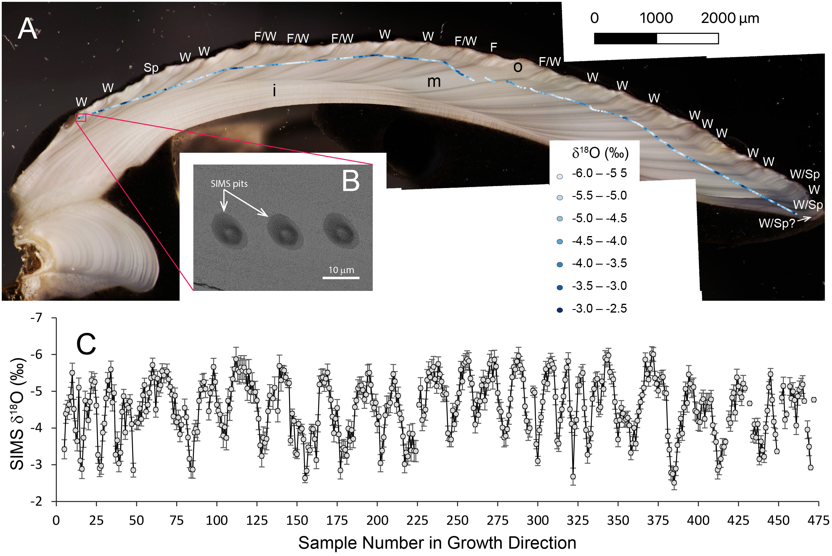
Figure 1 Photomicrograph of shell cross-section, location of SIMS sampling pits, SEM image of SIMS pits, and SIMS δ18Oshell values plotted using Quantum-GIS® software (QGIS.org, 2023). (A) Cross-section of specimen RFP3S-47 cut along the axis of maximum growth (umbo on left, growth margin on right; growth direction from left to right), showing 3 microstructural layers (i, inner layer; m, middle layer; o, outer layer) and light/dark couplets under reflected light hypothesized to represent annual increments. Approximately 22-24 light/dark couplets are visible. Sampling pits are identified in gradational shades of blue circles (enlarged from true size of 10 μm for ease of visibility), representing 0.5‰ intervals of SIMS δ18Oshell values where lighter blues represent lower values and darker blues are higher values. Estimated season of dark increment formation interpreted from the SIMS δ18Oshell time series (see text for details) are labeled as follows: W, winter; Sp, spring; F, Fall. The last dark increment nearest the growth margin does not include a SIMS δ18Oshell value; thus, the designation W/Sp? is estimated using the relative amount of shell growth from the date of harvest. Scale bar = 2000 μm. (B) SEM image of SIMS sampling pits at high resolution (5.5 k magnification) showing examples with no irregularities. Scale bar = 10 μm. (C) SIMS δ18Oshell values sampled along direction of growth (left to right). Gray circles are individual SIMS data points. Bars are standard deviations (2σ). Gaps represent data points removed during quality control.
SIMS analysis was performed at the University of Wisconsin-Madison WiscSIMS laboratory on a Cameca IMS 1280 in August 2018 during the same session as Moss et al. (2021) and following settings described in Wycech et al. (2018). Analysis pits ~10 μm in diameter and ~1 μm deep were sputtered using a 1.0 nA primary beam of 133Cs+. Three Faraday detectors in the double-focusing mass spectrometer simultaneously detected secondary ions of 16O−, 18O−, and 16OH−, with secondary 16O− count rates of ~2.4 Gcps. Values of δ18O are reported in permil (‰) relative to the VPDB (Vienna Pee Dee Belemnite) standard. Precision was determined as 2 times the standard deviation (s.d.) of repeated groups of bracketing measurements on the calcite running standard UWC-3, which averaged ±0.24‰ (2 s.d.) across the analysis session. Measured (raw) δ18O values were corrected to the VPDB scale for each group of 15–20 aragonite sample analyses following a 3-step procedure: 1. The instrumental bias of calcite on the VSMOW (Vienna Standard Mean Ocean Water) scale was calculated using the bracketing measurements of UWC-3. 2. An adjustment for the small difference in instrument bias (0.88‰) between calcite and aragonite analyses was applied based on calibration analyses of the aragonite standard UWArg-7 (δ18O = 19.73‰ VSMOW, Linzmeier et al., 2016) completed at the start of the analysis session. 3. Conversion from the VSMOW to VPDB scales followed procedures outlined in Coplen (1994).
The middle microstructural layer was targeted for SIMS analysis per Moss et al. (2021). SIMS analysis started nearest the umbo and proceeded along growth direction to the growth margin, sampling nearly the entire lifespan of the specimen and yielding 482 SIMS δ18Oshell values. Most of the shell was sampled by manual site selection along growth direction. To maximize machine time by sampling overnight, automated sampling of pre-selected points was implemented to capture the earliest ontogenetic years (40 samples) and the final ~8 light/dark couplets towards the growth margin (160 samples).
SIMS data were subjected to a quality-control protocol. First, analytical metrics of each sample measurement – including secondary ion yield, 16OH−/16O− ratio, and internal variability – were compared to the mean of the bracketing standards. 16OH−/16O− ratios ranged from 0.0129 to 0.0373, with an average of 0.0243 ± 0.0038 (1σ). Analyses were determined as outliers if they exhibited values that were above (below) the third (first) quartile by more than 1.5 times the interquartile range (Tukey, 1977), and were thus excluded from figures and interpretive discussion. This quality control removed 23 of the 482 total analyses (<5%). An additional 8 duplicate samples were removed from figures and interpretive discussion, resulting in 451 total SIMS δ18Oshell values. Next, SIMS pits were imaged by scanning electron microscopy (SEM) to screen for irregular pit shapes, cracks, or inclusions that may bias the δ18O data. For SEM imaging, the epoxy mount was loaded onto an aluminum receiver with double-sided copper tape. Images were taken using a Zeiss Supra 25 FESEM operating at 5.5 kV, using the SE2 detector, 30 μm aperture, and working distances of 12–15 mm (Carl Zeiss Microscopy, LLC, Peabody, MA). SEM images of SIMS analysis pits revealed no irregularities of either pit morphology or aragonite substrate (Figure 1B).
3 Results
3.1 SIMS δ18O values in A. borealis
SIMS δ18Oshell values in specimen RFP3S-47 exhibit a quasi-sinusoidal pattern (Figure 1C), with 24 cycles of local minima (−5.58 ± 0.32‰, 1σ) and maxima (−3.15 ± 0.39‰, 1σ) in agreement with the 24 light/dark couplets of annual growth increments visible under reflected light (Figure 1A). These SIMS δ18O values are comparable to the SIMS δ18O values measured from another Baltic Sea A. borealis specimen in Moss et al. (2021), where the authors noted a negative offset between their SIMS δ18Oshell values relative to coarser resolution IRMS δ18O values measured from the same specimen. Between 9 and 31 SIMS δ18Oshell measurements comprise a full couplet in specimen RFP3S-47, averaging 19 data points per couplet. Most dark increments occur at or near the highest SIMS δ18Oshell values (darker shades of blue circles locating SIMS pits on the shell cross-section in Figure 1A). Assuming one light/dark couplet represents an annual cycle, as is often the case in this species (Moss et al., 2018; Moss et al., 2021), our sampling interval equates to sub-monthly resolution on average (see Section 4.1 for further discussion of age modeling). However, we note that each discrete sample constitutes a 10 μm spot and a ~5 μm space between spots, and thus one-third of the shell along the sampling path is not represented by the samples presented in this study.
3.2 In situ temperature and salinity
Bottom water temperature (Figure 2A) and salinity (Figure 2B) were measured periodically at a location less than 2 km away from our study site (54.79169°N, 13.05831°E) using a calibrated CTD in a previous study (Zettler et al., 2017) between October 1976 and November 2017. The data span the approximate growth years of specimen RFP3S-47 based on counting couplets of light/dark growth increments (1977 to 2001). Prior to 1990, in situ temperature and salinity were measured at approximately seasonal resolution (n = 4 ± 1 per year). During and after 1990, the sampling frequency increased to an average of 7 ± 3 measurements per year. Throughout all years, eight months were sampled frequently, including the warmest (August) and coldest (March) months of the year (Figure 2C). However, there is a general dearth of data during the transitional months of April, June, September, and December.
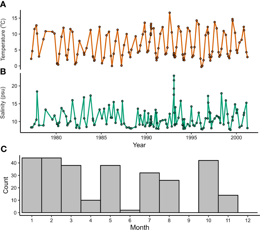
Figure 2 Environmental data measured less than 2 km from where specimen RFP3S-47 was collected (54°47’30.1”N, 13°03’29.9”E). (A, B) Bottom water temperature and salinity measured between 23-32 m depth. (C) Number of measurements taken in each month for all years of CTD data.
On average, bottom water temperatures ranged from 11.46 ± 2.63°C (1σ) in August to 2.28 ± 1.26°C in March, equating to an annual cycle of 9.18°C ± 3.89°C. However, we note that temperatures collected in July, August, and October are statistically indistinguishable from one another (ANOVA; n = 50, p = 0.41). The same is true for temperatures collected in February, March, and April (n = 46, p = 0.83). The highest bottom water temperature observed was 16.69°C on 5 August 1992, while the lowest temperature observed was −0.30°C on 13 February 1996. Bottom water salinity did not vary with the annual cycle. Salinity measurements exhibited a skewed-right distribution with a median value of 9.83 practical salinity units (psu). Significant deviations above average salinity occur frequently and sporadically throughout the sampling period, with a maximum value of 22.85 psu observed on 26 January 1993. Significant deviations below average salinity were lower in magnitude and frequency, with the minimum value of 7.67 psu observed on 7 May 1999.
4 Discussion
In this section, we demonstrate that the SIMS δ18Oshell dataset from specimen RFP3S-47 yields quantitative paleoclimate information, validating SIMS δ18Oshell values in A. borealis as a new climate archive for mid-to-high latitude coastal environments. First, to associate spatial changes in SIMS δ18Oshell values to temporal changes in environmental conditions, we apply an age-model (described in the next section) to the SIMS δ18Oshell data that aligns local δ18O maxima with the coldest winter months (Figure 3). We then correlate the age-modeled SIMS δ18Oshell dataset with in situ temperature and salinity data (Figure 4), as well as with the independent ORAS5 SST dataset (Zuo et al., 2019). These correlation analyses, in conjunction with the age model, show that variations in SIMS δ18Oshell values in specimen RFP3S-47 reflect regional hydroclimate conditions. Finally, we correlate the low-frequency variance component of the SIMS δ18Oshell dataset to interannual shifts in the NAO.
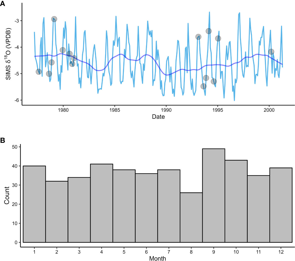
Figure 3 (A) Age-modeled SIMS δ18Oshell data from the (A) borealis specimen. Estimated growth dates are between March 1977 and May 2001. The light blue line is monthly-averaged δ18Oshell values, with gray dots indicating where values were linearly interpolated between bracketing months. The dark blue line represents the data passed through a 36-month LOWESS function. (B) Number of age-modeled growth months for SIMS δ18Oshell data (n = 290) for all growth years (n = 24). Most months (84%) are represented by one or two data points with no bias towards any particular time of year.

Figure 4 Age-modeled SIMS δ18Oshell values compared to in situ salinity measurements and two independent temperature datasets from the Baltic Sea. (A–D) Comparison of SIMS δ18Oshell values with in situ salinity (A, B) and temperature data (C, D) collected from shipboard measurements between October 1988 and May 2001 (Zettler et al., 2017), mean-averaged over seasonal intervals. (E, F) Comparisons of SIMS δ18Oshell values with sea surface temperature estimates for the entire Baltic Sea region extracted from the ORAS5-SST global reanalysis product at monthly resolution (Zuo et al., 2019). The δ18O axes in both (C, E) are inverted to better visualize variations in SIMS δ18Oshell values due to temperature. The dark green, blue, and red lines in (A, C, E) show each dataset passed through a 36-month LOWESS function. The equations in (D, F) are displayed to assess correlation, not as proxy calibrations for absolute temperature reconstruction. Parantheticals in each equation represent the standard error of the regression coefficients.
4.1 Age-modeled SIMS δ18Oshell values
A monthly age model was applied to all δ18Oshell samples throughout the lifespan of specimen RFP3S-47 by aligning the quasi-sinusoidal pattern to the annual cycle of temperature (as recorded by in situ CTD measurements) according to well-established methods (Beck et al., 1992; Klein et al., 1996; Surge et al., 2001). The age model assumes that local δ18Oshell maxima occur during the coldest winter months (January, February, March, and April, according to the ORAS5 SST dataset), with the final data point designated as the month of collection (May 2001). All samples between local maxima were assigned months based on linear interpolation of their position between bracketing maxima, which assumes a linear growth rate within years. Counting couplets of light and dark increments backwards from the collection date provides calendar years for all SIMS δ18Oshell samples. We thus infer relative variations in annual growth rates by examining the number of samples collected in each couplet of light and dark increments (Figure 5). Excluding the year of collection and the earliest growth year (which do not constitute full light/dark increment couplets), between 9 and 31 samples were collected per year, with periods of notably slow growth in the late 1970s and early 1990s. Given each sample constitutes one 10 μm spot and a ~5 μm space between samples, we can approximate an annual growth rate in μm per year (Figure 5, secondary y-axis). However, we caution that precisely quantifying growth rates requires a specific protocol where measurements are made perpendicular to growth lines bounding growth increments along the direction of growth (Schöne et al., 2005) and often the hinge plate is used to avoid any biases imparted by the conchoidal shape of the major growth axis (e.g., Winkelstern et al., 2013; Palmer et al., 2021). Given that calculating annual growth rate was not the primary focus of this study and the sampling scheme used did not follow the necessary protocol for such an analysis, our statistical approach provides a relative estimate of growth rates that compliments the more thorough growth assessments of A. borealis specimens conducted by Moss et al. (2018); Moss et al. (2021).
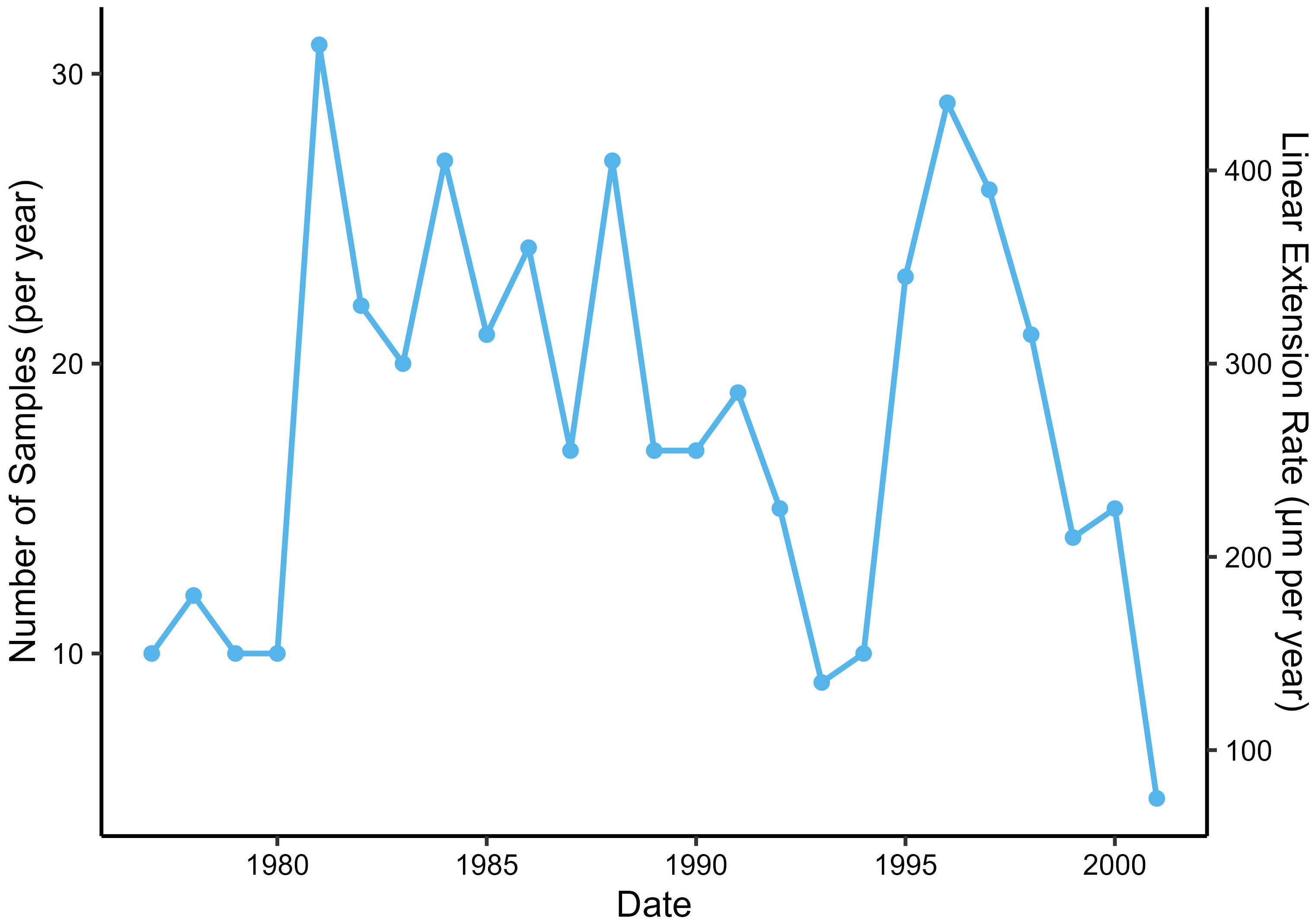
Figure 5 Number of data points sampled from specimen RFP3S-47 for each calendar year between the year of collection (2001) and the earliest ontogenetic year (1977). Years were assigned to each growth increment by counting couplets of light and dark increments backwards from the year of collection.
For specimen RFP3S-47, all 24 local δ18Oshell maxima occur at or near the dark increment, indicating formation during cold months (i.e., late fall, winter, or early spring; Figure 1A). While not a ubiquitous feature for all bivalves across all latitudes, the coincident timing of dark increment formation with δ18Oshell maxima has been observed in other mid- to high-latitude bivalves, including Arctica islandica (Witbaard et al., 1994; Schöne et al., 2004) and Mercenaria mercenaria (Elliot et al., 2003). Fifteen local δ18Oshell maxima occur exactly at the dark increment (i.e., winter); three occur slightly before the dark increment (i.e., late fall); and six occur slightly after the dark increment (i.e., early spring). Once all data points were age modeled, we calculated that each analysis (10 μm spot and ~5 μm space) represents on average 19.5 days.
After the age model was applied, δ18Oshell values were mean-averaged over monthly intervals between March 1977 and April 2001 (Figure 3A). Data points are distributed almost uniformly across months, which is a function of both our high sampling resolution and the inherent assumption of constant growth in our age model (Figure 3B). Out of 290 months in the time series, 141 are represented by one data point, 103 are represented by two data points, 21 are represented by three data points, 9 are represented by four data points, and one is represented by 5 data points. Only 15 months in the time series were unrepresented by any δ18Oshell samples. For these months, δ18Oshell values were linearly interpolated between bracketing months (gray dots, Figure 3A).
Once the data were averaged into monthly intervals, a 36-month locally weighted scatterplot smoothing (LOWESS) function was applied to highlight the low-frequency variance component (dark blue line, Figure 3A). The LOWESS function (Cleveland, 1979) is a non-parametric regression method that replaces each data point in a time series with a weighted average based on a specified window size and the values of the data points in close proximity to the central data point in that window. For the age-modeled SIMS δ18Oshell time series, we applied a 36-point window size (i.e., a 36-month bandwidth), which is the minimum bandwidth required to mitigate any effects due to seasonality. These smoothed data accentuate interannual variability that peaks within the 3-to-4-year bandwidth over the 24-year time series. The magnitude of the interannual oscillations vary widely, with a few anomalous periods exhibiting cycles as large as 0.64 and 0.76‰ (troughs in 1984 and 1990) or as small as 0.05‰ (troughs in 1993 and 1996). Average interannual variability (0.35‰) in the age-modeled SIMS δ18Oshell dataset is an order of magnitude lower than average seasonal variability (2.43‰). However, interannual variability appears to modulate the seasonal cycle, resulting in seasonal amplitudes as large as 3.31‰ (1997) or as low as 1.44‰ (1990).
4.2 Correlating SIMS δ18Oshell values to temperature and salinity
To explore the mechanisms behind the apparent seasonal and interannual variability, age-modeled SIMS δ18Oshell values were compared to salinity and two separate temperature datasets from the Baltic Sea region (Figure 4). Although we have correlated age-modeled SIMS δ18Oshell values to two different temperature datasets, we establish this correlation strictly to assess for mechanisms of seasonal and interannual variability. As discussed in Moss et al. (2021), SIMS δ18Oshell values cannot be used to reconstruct absolute temperatures in A. borealis shells. Offsets between SIMS-measured δ18O and IRMS-measured δ18O values, which are used in temperature calibrations, are reported in a variety of calcite and aragonite biogenic carbonates. The cause of these offsets, commonly <1‰, can be due to a variety of factors (Helser et al., 2018; Wycech et al., 2018), including possible inclusion of water or organic material in the carbonate matrix. Here, we do not attempt to characterize or calibrate the absolute δ18O value from these samples, but instead use the quality-controlled analytical metrics as the basis for our assumption that SIMS faithfully measures relative changes of δ18O values in specimen RFP3S-47.
Further complications associated with reconstructing temperatures from absolute SIMS δ18Oshell values presented here arise from unconstrained δ18Owater values at this location throughout the study period. Although studies have correlated δ18Owater values to salinity in the Baltic Sea (Frohlich et al., 1988; Harwood et al., 2008), the strength of this correlation is likely variable in space and time. However, given that δ18Oshell values are primarily a function of temperature and the δ18O value of ambient water, we demonstrate the utility of the combined signal in assessing modes of seasonal to interannual climate variability in the Baltic Sea region. As a general rule, we define strong correlations as those with an r2 value greater than 0.50 (|r| > 0.70), moderate correlations as those with an r2 value greater than 0.1 (0.3 < |r| < 0.7), and weak correlations as those with an r2 value less than 0.1 (|r| < 0.3).
Salinity and temperature depicted in Figure 4A through 4D were measured simultaneously via shipborne CTD measurements less than two kilometers from our study site, hereafter referred to as in situ salinity and temperature (Zettler et al., 2017; see Section 3.2). Although in situ water data extend back to the earliest estimated growth month for specimen RFP3S-47 (March 1977), the CTD sampling rate is too sparse to support analysis of subannual variance. Therefore, only in situ water data collected between October 1988 and May 2001 were used for comparison to age-modeled SIMS δ18Oshell values. To facilitate comparison, age-modeled SIMS δ18Oshell values and in situ salinity and temperature were mean-averaged into seasonal values (Winter = DJF, Spring = MAM, Summer = JJA, Fall = SON). The temperature dataset depicted in Figures 4E, F was compiled from the ORAS5 SST global reanalysis product (Zuo et al., 2019). The ORAS5 product was chosen above other readily available global SST products primarily for two reasons. First, it is calculated at sufficient spatiotemporal resolution (monthly; 1° x 1°) with reliable data at high latitudes, allowing us to integrate 49 grid-points into a single regional SST estimate for the Baltic Sea (Figure 6). Second, ORAS5 is a data assimilation product that tunes the output of the European Centre for Medium-Range Weather Forecasts’ OCEAN5 system to in situ observations. Thus, it is well-informed by remote and in situ observations, particularly in this dynamic high-latitude coastal region (Carton et al., 2019; Zuo et al., 2019). This is demonstrated by a strong correlation between in situ temperature and ORAS5 SST when both datasets are seasonally averaged (n = 51, r2 = 0.82, p < 0.001). The correlation between SIMS δ18Oshell values and each dataset are as follows: no correlation for in situ salinity (r2 = -0, n = 51, p = 0.99), strong for in situ temperature (r2 = 0.52, n = 51, p < 0.001), and moderate for the ORAS5 dataset (r2 = 0.42, n = 290, p < 0.001).
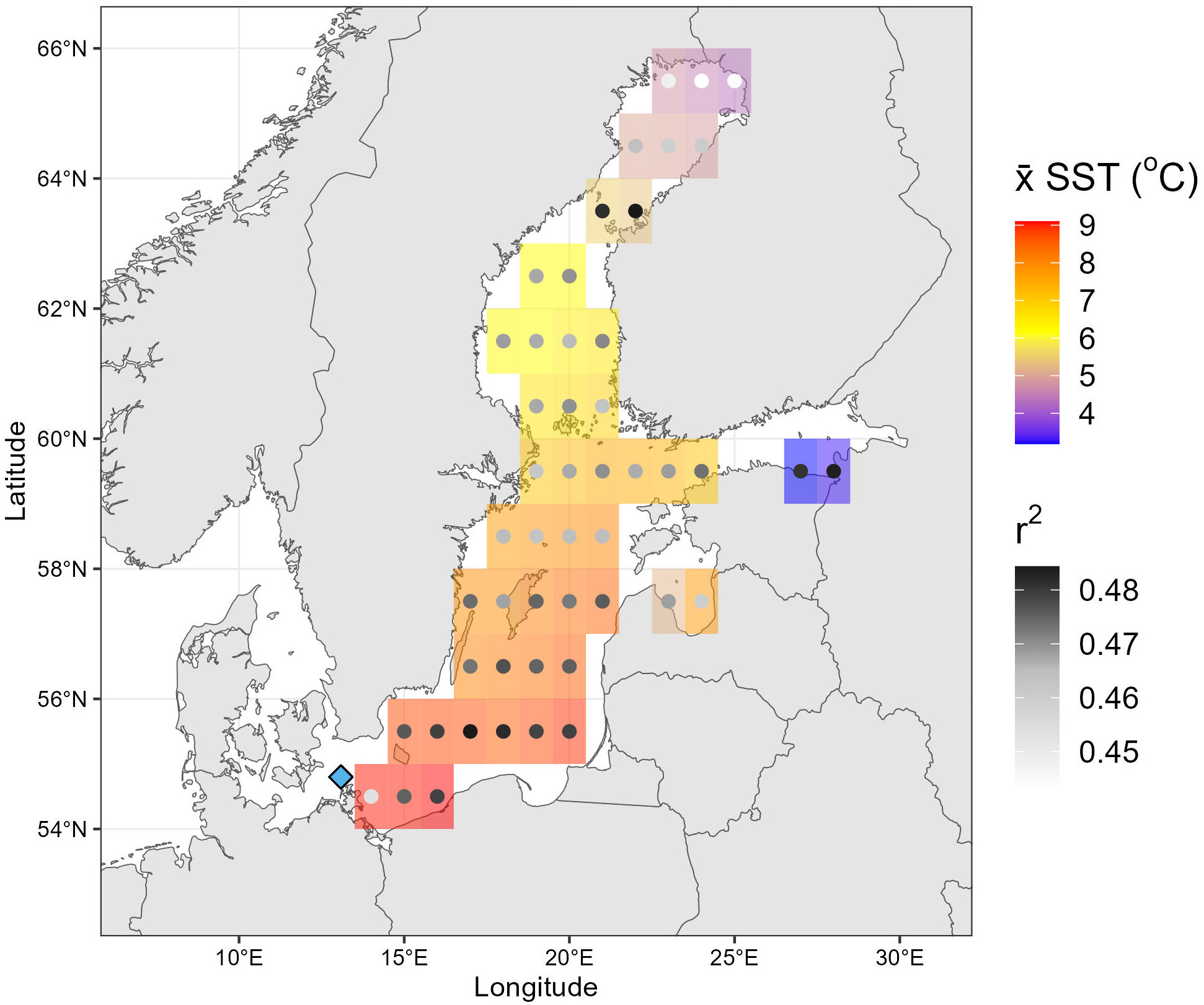
Figure 6 Spatial correlation analysis between the SIMS δ18Oshell data and Baltic Sea SST estimates derived from the ORAS5 SST dataset. Mean SST (x̅SST; shaded region) and the Pearson correlation coefficients (r2; points) are shown for each grid point. The blue diamond marks our study site, where specimen RFP3S-47 was collected. The color of each point denotes the r2 value between age-modeled SIMS δ18Oshell values and SST at that specific location throughout the entire study period (March 1977 to May 2001). The shaded region behind each point indicates the x̅SST over the entire study period.
Both temperature datasets exhibit a moderate-to-strong correlation with age-modeled SIMS δ18Oshell values (Pearson’s correlation coefficient, p < 0.001). Given the assumptions of our age model (aligning local SIMS δ18O maxima to in situ temperature minima), this finding suggests that monthly SIMS δ18Oshell values in specimen RFP3S-47 are varying in part with in situ and regional-scale temperature variability, and that temperatures at ~30m depth in the southwest corner of the Baltic Sea covary significantly with SSTs across the entire Baltic Sea. Furthermore, the standard error of the regression coefficients (parantheticals in regression equations, Figures 4D, F) overlap between the two temperature models, suggesting the relationship between SIMS δ18O and both temperature datasets is similar. However, a Wilcoxon Rank Sum Test (Bauer, 1972) performed on the regression coefficeints from 10,000 bootstrapped resamples suggests that these two equations are statistically distinct (p < 0.001). We also note that the slopes of both SIMS δ18O – temperature equations are substantially lower than those that are typically observed in other bivalves using IRMS (e.g., −0.22‰; Dettman et al., 1999). We postulate that the lower slope of the relationship between SIMS δ18Oshell values in specimen RFP3S-47 to temperature could be attributed to ontogenetic (growth-related) effects, destructive interference of the temperature signal by δ18Owater values, and by potential seasonal growth cessations (stops).
Ontogenetic effects have been observed in many bivalve species, where the degree to which δ18Oshell values capture the full range of seasonal variation decreases with age (Goodwin et al., 2003). However, our results are not consistent with these ontogenetic effects in specimen RFP3S-47, as neither the amplitude of δ18Oshell couplets nor the number of SIMS δ18Oshell measurements constituting each couplet show a secular negative trend. Therefore, we assume that SIMS δ18Oshell values are capturing the same range of the annual cycle through all growth years and thus do not impose any artifacts on interannual variability.
Variable δ18Owater values could reduce the apparent temperature sensitivity in age-modeled SIMS δ18Oshell values if warmer (cooler) temperatures coincide with higher (lower) δ18Owater values. Previous work has shown that δ18Owater values in the Baltic Sea region are tightly coupled with salinity (Frohlich et al., 1988), and thus could be used as a proxy for δ18Owater values. However, the poor correlation between salinity and the age-modeled SIMS δ18Oshell dataset on seasonal timescales indicate that the relationship between the two at our site is complex. Additionally, we find that adding both temperature and salinity as predictor variables for age-modeled SIMS δ18Oshell values does not yield better estimates than temperature alone (r2 = 0.52, p < 0.001). Therefore, we cannot use salinity on seasonal timescales to robustly test whether variations in δ18Owater values are diminishing the temperature sensitivity of SIMS δ18Oshell values. Regardless, we examined the relationship between in situ temperature and salinity to verify if seasonal changes in salinity (used here as a proxy for δ18Owater) could influence the slope of the relationship between SIMS δ18Oshell values and temperature (Figure S1 and Table S1). We find the correlation between in situ salinity and temperature is extremely weak (Figure S1; n = 146, r2 = 0.02, n = 0.14), and there are no significant differences in salinities collected between summer and winter months (Table S1). While it is likely that SIMS δ18Oshell values are influenced by variations in δ18Owater values, the lack of seasonal variation in salinity (serving here as a proxy for δ18Owater) suggests that the influence of δ18Owater variability on SIMS δ18Oshell values is stochastic rather than systematic. Therefore, we find it highly unlikely that δ18Owater variations can explain the reduced slope in the correlation between SIMS δ18Oshell values and temperature.
Seasonal growth cessations (or stops in growth) and slow downs induced by exceeding growth temperature thresholds are a well-documented phenomena in many bivalve species (e.g., Ansell, 1968; Jones and Quitmyer, 1996; Fritz, 2001 and references therein). It is estimated that Baltic Sea A. borealis exhibits an upper temperature threshold between 14 – 17°C and a lower temperature threshold between 0 – 4°C (Oertzen, 1973; Oertzen and Schulz, 1973). Our in situ temperature dataset indicates that specimen RFP3S-47 rarely experienced summer temperatures approaching this upper temperature threshold but regularly experienced winter temperatures in the lower threshold range. Furthermore, other environmental and physiological factors can also influence seasonal growth cessation (see Moss et al., 2018 for an overview). Moss et al. (2021) report that temperature stress during cool months could explain the growth slow downs observed in Baltic Sea A. borealis during that time; however, winter/spring spawning events could not be ruled out as a possibility.
Seasonal growth cessations would manifest as truncated seasonal amplitudes in δ18Oshell values and, thus, a reduced slope in the correlation between SIMS δ18Oshell values and temperature. To test if seasonal growth cessations were occuring, we conducted two separate statistical analyses. First, if growth cessations were occuring in the winter months, we would expect less variance in SIMS δ18Oshell values during winter months (DJFM = December, January, February, March) than in summer months (JJAS = June, July, August, September). However, we find no significant difference in variance between winter and summer SIMS δ18Oshell values (n = 193, p = 0.58). For the second analysis, we compared the correlation between in situ temperature and SIMS δ18Oshell values collected between summer and winter months. We expect that, if growth cessations were occurring during the cold season, winter SIMS δ18O values would exhibit a weaker correlation with temperature than summer values. However, results are sensitive to which temperature dataset is used. Using the seasonally averaged in situ temperature dataset, we find no significant correlation between SIMS δ18Oshell values and in situ temperatures for neither winter months (n = 24, r2 < 0.01, p = 0.95) nor summer months (n = 24, r2 = 0.08, p = 0.17). Using the ORAS5 SST dataset, we find a stronger correlation between temperature and winter SIMS δ18Oshell values (n = 97, r2 = 0.36, p < 0.001) than summer values (n = 96, r2 = 0.03, p = 0.07). However, we would expect this stronger correlation due to increased turnover of the Baltic Sea in the winter months, and thus specimen RFP3S-47 at ~30m depth would likely experience temperatures more similar to Baltic Sea SSTs during the cold season. The inconclusive statistical analyses conducted here, and the difficulty with determining growth cessations via visual inspection, means we cannot rule out that growth cessations are reducing the slope in the correlation between temperature and SIMS δ18Oshell values.
Age-modeled SIMS δ18Oshell values exhibit the greatest interannual variability of all datasets presented in this study, with apparent oscillations occurring every three to four years. Although interannual variability is an order of magnitude smaller than annual variability in the SIMS δ18Oshell dataset, and interannual variability makes up an even smaller component of the environmental datasets, we find that correlating the interannual components of each dataset yields different results than correlating the monthly- and seasonally-averaged datasets. First, seasonal SIMS δ18Oshell values and in situ salinity are strongly correlated when both datasets are passed through a 36-month LOWESS function (r2 = 0.71, n = 51, p < 0.001). The correlation between seasonal SIMS δ18O and in situ temperature actually decreases when we execute the same comparison (r2 = 0.05, n = 51, p = 0.13), and this same decrease is observed to a lesser extent when comparing the smoothed monthly SIMS δ18O data and ORAS5 SSTs (r2 = 0.29, n = 290, p < 0.001). These analyses suggest that, while temperature imposes a strong seasonal effect on δ18Oshell values, salinity is predominantly driving interannual variability.
4.3 SIMS δ18Oshell values and the NAO
Given the strong influence of temperature and salinity on the SIMS δ18Oshell values at different timescales, we suggest that δ18Oshell values in A. borealis from the Baltic Sea may be used to reflect changes in the NAO. The NAO imposes a strong effect on regional temperatures and hydrology as one of the leading modes of interannual climate variability in northern Europe (Hurrell, 1995; Jones et al., 2003). The Baltic Sea is particularly sensitive to the NAO, with stronger (weaker) westerlies bringing increased (decreased) storminess and warmer (colder) winters to the region during the positive (negative) phase (Hurrell, 1995; Lehmann et al., 2011). Because the NAO exhibits a temporal periodicity of approximately 3–4 years, we hypothesize that NAO-related climate changes would work to simultaneously increase SST while decreasing δ18Owater values (and vice versa), effects that would compound to increase the amplitude of the interannual δ18Oshell response of A. borealis in the Baltic Sea.
To test this hypothesis, we compared the age-modeled SIMS δ18Oshell dataset from specimen RFP3S-47 to the NAO index for the entire study period (Figure 7A). Here, the NAO index is defined as the normalized difference in sea level pressure between Iceland and the Azores (Rogers, 1984; Hurrell, 1995). Additionally, to determine if SIMS δ18Oshell values could track significant changes in the NAO, we conducted a change point analysis on both monthly datasets using the pruned exact linear time (PELT) method (Killick et al., 2012), which is the optimal method for finding exact solutions in change point detection (Truong et al., 2020). These change points are shown in Figure 7A as blue diamonds on the δ18O time series and black diamonds on the NAO time series. Although the two datasets are uncorrelated at monthly intervals (r2 = 0.002, p = 0.49), they are moderately inversely correlated when each monthly dataset are passed through a 36-month LOWESS function (r2 = 0.46, n = 290, p < 0.001; Figure 7A). This change in correlation between monthly and interannual timescales observed between SIMS δ18Oshell values and the NAO is very similar to the change in correlation observed between SIMS δ18O and salinity. However, we note that the correlation between SIMS δ18Oshell values and the NAO is supported by a much larger sample size due to the higher resolution (monthly vs. seasonal) from which the smoothed data were derived.
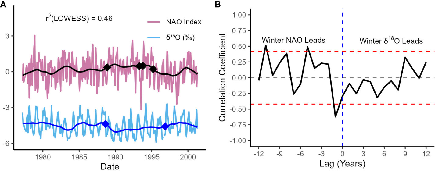
Figure 7 SIMS δ18Oshell values compared to the North Atlantic Oscillation (NAO). (A) Age-modeled SIMS δ18Oshell values (blue) and the NAO Index (purple), defined as the normalized difference in sea-level pressures between Iceland and the Azores. The bold blue and black lines represent each dataset passed through a 36-month LOWESS function. Diamonds indicate change points in each monthly time series, identified using a PELT change point detection method. (B) Lagged correlation analysis between winter (DJFM) SIMS δ18Oshell values and the NAO Index. The x-axis values represent the number of years that the NAO lags SIMS δ18Oshell values. The red-dotted lines (r = ± 0.42) indicate the point at which the correlation becomes significant at the 95% confidence level (Hu et al., 2017).
The strength of the correlation between the smoothed SIMS δ18Oshell dataset and the NAO is such that SIMS δ18Oshell values track a documented regime shift in the NAO circa 1989 (Figure 7A; first black/blue diamonds), where the overall trend in the NAO shifts towards more negative values while winter NAO values remain largely positive (Lehmann et al., 2011). Moreover, the 1989 regime shift is visually striking, particularly in both LOWESS-smoothed time series. The other change point in the SIMS δ18O time series (circa 1996) occurs within three years of a cluster of change points in the NAO time series, which are associated with a pronounced negative excursion (1994) and an interannual shift towards more negative values (1995). All these latter change points are detected nearly within a 36-month window of each other, which lends further support to our conclusion that δ18Oshell values covary with the NAO on interannual timescales.
The significant correlation on interannual timescales between the NAO index and the SIMS δ18Oshell dataset suggests that positive (negative) phases of the NAO generally bring warmer (cooler) and wetter (dryer) conditions to the Baltic Sea. This finding is consistent with previous studies analyzing modeled and observed temperature and salinity data from the Baltic Sea (Hänninen et al., 2000; Lehmann et al., 2011). In summary, warmer winter SSTs are associated with positive phases of the NAO, as stronger westerly winds bring milder winters and excess precipitation to the region (Hurrell, 1995; Lehmann et al., 2011). Negative phases of the NAO are associated with weaker westerly winds, more extreme winters, and less precipitation in northern Europe (Dickson and Brander, 1993). Additionally, pulses of saline water from the North Sea through the Danish Straits are more likely to occur during a negative NAO phase (Schinke and Matthäus, 1998). Thus, opposite phases of the NAO propagate conditions where temperature and freshwater flux reinforce one another on interannual timescales, likely amplifying the environmental signal recorded in the SIMS δ18Oshell dataset.
To evaluate the mechanisms behind the correlation between the NAO Index and the SIMS δ18Oshell dataset, particularly during winter when the NAO exhibits the greatest regional impact, we conducted a lagged correlation analysis between winter values (DJFM) from both datasets (Figure 7B). We find that winter values from each dataset are moderately correlated when winter NAO leads winter δ18Oshell values by one year (r2 = 0.39, n = 23, p = 0.002). The significant lagged correlation between winter SIMS δ18Oshell values and the NAO could be attributed to the stepwise hydrologic response observed across the Baltic Sea region to freshwater forcing from the NAO. Freshwater runoff into the Baltic Sea lags the NAO index by a few months, with salinity lagging further behind freshwater runoff within one year (Hänninen et al., 2000). The spread in these lag times is largely due to the broad range of residence times (hours to years) that water exhibits across the Baltic Sea region, both in the Baltic Sea itself and in its various watersheds (Ehlin, 1981; Bergström and Carlsson, 1994; Hänninen et al., 2000). Given that our site is located in the Arkona basin subregion near the mouth of the Baltic Sea, we hypothesize that the SIMS δ18Oshell dataset is capturing an integrated signal of freshwater flux derived from melting snow and ice, the volume of which is largely controlled by the state of previous years’ NAO. This hydroclimatic link between the NAO and SIMS δ18Oshell values on interannual timescales is further supported by the significant correlation between SIMS δ18Oshell values and in situ salinity when both datasets are binned annually and salinity leads by one-year (Figure S2; n = 23, r2 = 0.29, p = 0.007). We observe that the lagged correlation analysis conducted specifically on winter δ18Oshell values and the NAO index exhibits a higher coefficient of determination than the lagged correlation analysis conducted between annually binned δ18Oshell values and salinity. We postulate this could be due to: (a) the coarser sampling resolution in the in situ salinity dataset precluding a winter-only comparison with SIMS δ18Oshell values, and (b) the influence of the NAO index on both temperature and δ18Owater.
5 Conclusions
This study presents the first multidecadal δ18O time series generated from an A. borealis shell using SIMS. At sub-monthly resolution, we find that the SIMS δ18Oshell time series is significantly correlated to in situ temperatures at the mouth of the Baltic Sea (r2 = >0.52), as well as regional SST across the Baltic Sea based on ORAS5 SST estimates (r2 = 0.42). The strongest correlation emerges when comparing the interannual components of the SIMS δ18Oshell dataset and salinity (r2 = 0.71). We observe a moderate correlation between the interannual components of the SIMS δ18Oshell dataset and the NAO Index (r2 = 0.46), where SIMS δ18Oshell values capture a well-documented regime shift circa 1989 (Lehmann et al., 2011). We hypothesize that this coupling emerges as a result of NAO-related climate effects creating constructive interference between SST and δ18Owater values at the southern margin of the Baltic Sea on interannual timescales, thereby imposing a strong environmental signal onto the SIMS δ18Oshell dataset. The integrated hydroclimate signal captured at our site by the SIMS δ18Oshell dataset is further supported by a significant correlation between binned DJFM winter δ18Oshell values with the previous years’ winter NAO Index (r2 = 0.39). Our analyses indicate that SIMS δ18Oshell values in A. borealis from the Baltic Sea are a potentially rich source of paleoclimate information, with capabilities of reconstructing the mid-to-high latitude component of the NAO during the Holocene at sub-monthly resolution over decadal timescales.
Data availability statement
The original contributions presented in the study are included in the article/Supplementary Material. Further inquiries can be directed to the corresponding author.
Author contributions
HH: Conceptualization, Formal Analysis, Visualization, Writing – original draft, Writing – review & editing. DS: Conceptualization, Funding acquisition, Investigation, Project administration, Visualization, Writing – original draft, Writing – review & editing. IO: Data curation, Investigation, Visualization, Writing – review & editing. MZ: Investigation, Writing – review & editing. DM: Investigation, Writing – review & editing.
Funding
The author(s) declare financial support was received for the research, authorship, and/or publication of this article. Funding for this study was provided by the US National Science Foundation (NSF) to Surge (#EAR-1656974). The WiscSIMS Laboratory is supported by the US NSF (Grant #EAR-1355590 and EAR-1658823). Long-term environmental data for Figures 2A, B were obtained within the framework of the German Baltic Sea Monitoring financed by the Federal Maritime and Hydrographic Agency (BSH) and carried out by the Leibniz Institute for Baltic Sea Research (IOW).
Acknowledgments
Dr. Jonathan Lees is gratefully acknowledged for his helpful suggestions towards analyzing temporal variations in the SIMS δ18Oshell dataset. We also thank Garrett Braniecki for helpful insights into analyzing growth variations in specimen RFP3S-47. Comments from three reviewers helped improve this manuscript and were greatly appreciated.
Conflict of interest
The authors declare that the research was conducted in the absence of any commercial or financial relationships that could be construed as a potential conflict of interest.
Publisher’s note
All claims expressed in this article are solely those of the authors and do not necessarily represent those of their affiliated organizations, or those of the publisher, the editors and the reviewers. Any product that may be evaluated in this article, or claim that may be made by its manufacturer, is not guaranteed or endorsed by the publisher.
Supplementary material
The Supplementary Material for this article can be found online at: https://www.frontiersin.org/articles/10.3389/fmars.2023.1293823/full#supplementary-material
References
Ansell A. D. (1968). The Rate of Growth of the Hard Clam Mercenaria mercenaria L) throughout the Geographical Range. ICES J. Mar. Sci. 31, 364–409. doi: 10.1093/icesjms/31.3.364
Bauer D. F. (1972). Constructing confidence sets using rank statistics. J. Am. Stat. Assoc. 67, 687–690. doi: 10.1080/01621459.1972.10481279
Beck J. W., Edwards R. L., Ito E., Taylor F. W., Recy J., Rougerie F., et al. (1992). Sea-surface temperature from coral skeletal strontium/calcium ratios. Science 257, 644–647. doi: 10.1126/science.257.5070.644
Carton J. A., Penny S. G., Kalnay E. (2019). Temperature and salinity variability in the SODA3, ECCO4r3, and ORAS5 ocean reanalyses 1993–2015. J. Clim. 32, 2277–2293. doi: 10.1175/JCLI-D-18-0605.1
Clark G. R. (1974). Growth lines in invertebrate skeletons. Ann. Rev. Earth Planet Sci. 2, 77–99. doi: 10.1146/annurev.ea.02.050174.000453
Cleveland W. S. (1979). Robust locally weighted regression and smoothing scatterplots. J. Am. Stat. Assoc. 74, 829–836. doi: 10.1080/01621459.1979.10481038
Coplen T. B. (1994). Reporting of stable hydrogen, carbon, and oxygen isotopic abundances (Technical Report). Pure Appl. Chem. 66, 273–276. doi: 10.1351/pac199466020273
Dettman D. L., Lohmann K. C. (1993). Seasonal change in Paleogene surface water δ18O: Fresh-water bivalves of Western North America. Eds. Swart P. K., Lohmann K. C., Mckenzie J., Savin S. (Washington, DC: American Geophysical Union), 153–163.
Dettman D. L., Lohmann K. C. (1995). Microsampling carbonates for stable isotope and minor element analysis: physical separation of samples on a 20 micrometer scale. J. Sed. Res. 65A, 566–569. doi: 10.1306/D426813F-2B26-11D7-8648000102C1865D
Dettman D. L., Reische A. K., Lohmann K. C. (1999). Controls on the stable isotope composition of seasonal growth bands in aragonitic fresh-water bivalves (unionidae). Geochim. Cosmochim. Acta 63, 1049–1057. doi: 10.1016/S0016-7037(99)00020-4
Dickson R. R., Brander K. M. (1993). Effects of a changing windfield on cod stocks of the North Atlantic. Fish. Oceanogr. 2, 124–153. doi: 10.1111/j.1365-2419.1993.tb00130.x
Dunca E., Mutvei H., Göransson P., Mörth C.-M., Schöne B. R., Whitehouse M. J., et al. (2009). Using ocean quahog (Arctica islandica) shells to reconstruct palaeoenvironment in Öresund, Kattegat and Skagerrak, Sweden. Int. J. Earth Sci. 98, 3–17. doi: 10.1007/s00531-008-0348-6
Ehlin U. (1981). “Hydrology of the Baltic Sea,” in Elsevier Oceanography Series. Ed. Voipio A. (Amsterdam: Elsevier).
Elliot M., Demenocal P. B., Linsley B. K., Howe S. S. (2003). Environmental controls on the stable isotopic composition of Mercenaria mercenaria: Potential application to paleoenvironmental studies. Geochem. Geophys. Geosyst. 4, 1–16. doi: 10.1029/2002GC000425
Fritz L. W. (2001). “Chapter 2 Shell structure and age determination,” in Developments in Aquaculture and Fisheries Science. Eds. Kraeuter J. N., Castagna M. (Amsterdam: Elsevier).
Frohlich K., Grabczak J., Rozanski K. (1988). Deuterium and oxygen-18 in the Baltic Sea. Chem. Geol. 72, 77–83. doi: 10.1016/0168-9622(88)90038-3
Goodwin D. H., Flessa K. W., Schöne B. R., Dettman D. L. (2001). Cross-calibration of daily growth increments, stable isotope variation, and temperature in the Gulf of California bivalve Mollusk Chione Cortezi: implications for paleoenvironmental analysis. PALAIOS 16 (4), 387–398. doi: 10.1669/0883-1351(2001)016<0387:CCODGI>2.0.CO;2
Goodwin D. H., Gillikin D. P., Jorn E. N., Fratian M. C., Wanamaker A. D. (2021). Comparing contemporary biogeochemical archives from Mercenaria mercenaria and Crassostrea virginica: Insights on paleoenvironmental reconstructions. Palaeogeogr. Palaeocl. 562, 110110. doi: 10.1016/j.palaeo.2020.110110
Goodwin D. H., Schöne B. R., Dettman D. L. (2003). Resolution and fidelity of oxygen isotopes as paleotemperature proxies in bivalve Mollusk shells: models and observations. PALAIOS 18, 110–125. doi: 10.1669/0883-1351(2003)18<110:RAFOOI>2.0.CO;2
Hänninen J., Vuorinen I., Hjelt P. (2000). Climatic factors in the Atlantic control the oceanographic and ecological changes in the Baltic Sea. Limnol. Oceanogr. 45, 703–710. doi: 10.4319/lo.2000.45.3.0703
Harwood A. J. P., Dennis P. F., Marca A. D., Pilling G. M., Millner R. S. (2008). The oxygen isotope composition of water masses within the North Sea. Estuar. Coast. 78, 353–359. doi: 10.1016/j.ecss.2007.12.010
Helser T. E., Kastelle C. R., Mckay J. L., Orland I. J., Kozdon R., Valley J. W. (2018). Evaluation of micromilling/conventional isotope ratio mass spectrometry and secondary ion mass spectrometry of δ18O values in fish otoliths for sclerochronology. Rapid Commun. Mass. Sp. 32, 1781–1790. doi: 10.1002/rcm.8231
Hu J., Emile-Geay J., Partin J. (2017). Correlation-based interpretations of paleoclimate data–where statistics meet past climates. Earth Planet. Sc. Lett. 459, 362–371. doi: 10.1016/j.epsl.2016.11.048
Hurrell J. (1995). Decadal trends in the North Atlantic oscillation: regional temperatures and precipitation. Science 269, 676–679. doi: 10.1126/science.269.5224.676
Jones P. D., Osborn T. J., Briffa K. R. (2003). Pressure-based measures of the north Atlantic oscillation (NAO): A comparison and an assessment of changes in the strength of the NAO and in its influence on surface climate parameters. North Atlantic Oscillation: Climatic Significance Environ. Impact. 134, 51–62. doi: 10.1029/134GM03
Jones D. S., Quitmyer I. R. (1996). Marking time with bivalve shells: oxygen isotopes and season of annual increment formation. PALAIOS 11, 340–346. doi: 10.2307/3515244
Jones D. S., Williams D. F., Arthur M. A. (1983). Growth history and ecology of the Atlantic surf clam, Spisula solidissima (Dillwyn), as revealed by stable isotopes and annual shell increments. J. Exp. Mar. Biol. Ecol. 73, 225–242. doi: 10.1016/0022-0981(83)90049-7
Killick R., Fearnhead P., Eckley I. A. (2012). Optimal detection of changepoints with a linear computational cost. J. Am. Stat. Assoc. 107, 1590–1598. doi: 10.1080/01621459.2012.737745
Klein R. T., Lohmann K. C., Thayer C. W. (1996). Bivalve skeletons record sea-surface temperature and δ18O via Mg/Ca and 18O/16O ratios. Geology 24, 415–418. doi: 10.1130/0091-7613(1996)024<0415:BSRSST>2.3.CO;2
Kozdon R., Ushikubo T., Kita N. T., Spicuzza M., Valley J. W. (2009). Intratest oxygen isotope variability in the planktonic foraminifer N. pachyderma: Real vs. apparent vital effects by ion microprobe. Chem. Geol. 258, 327–337. doi: 10.1016/j.chemgeo.2008.10.032
Lehmann A., Getzlaff K., Harlaß J. (2011). Detailed assessment of climate variability in the Baltic Sea area for the period 1958 to 2009. Clim. Res. 46, 185–196. doi: 10.3354/cr00876
Linzmeier B. J., Kozdon R., Peters S. E., Valley J. W. (2016). Oxygen isotope variability within nautilus shell growth bands. PloS One 11, e0153890. doi: 10.1371/journal.pone.0153890
Matta M. E., Orland I. J., Ushikubo T., Helser T. E., Black B. A., Valley J. W. (2013). Otolith oxygen isotopes measured by high-precision secondary ion mass spectrometry reflect life history of a yellowfin sole (Limanda aspera). Rapid Commun. Mass. Sp. 27, 691–699. doi: 10.1002/rcm.6502
Moss D. K., Ivany L. C., Judd E. J., Cummings P. W., Bearden C. E., Kim W.-J., et al. (2016). Lifespan, growth rate, and body size across latitude in marine Bivalvia, with implications for Phanerozoic evolution. Proc. R. Soc. Lond. 283 (1836), 20161364. doi: 10.1098/rspb.2016.1364
Moss D. K., Surge D., Khaitov V. (2018). Lifespan and growth of Astarte borealis (Bivalvia) from Kandalaksha Gulf, White Sea, Russia. Polar Biol. 41, 1359–1369. doi: 10.1007/s00300-018-2290-9
Moss D. K., Surge D., Zettler M. L., Orland I. J., Burnette A., Fancher A. (2021). Age and growth of Astarte borealis (Bivalvia) from the Southwestern Baltic Sea using secondary ion mass spectrometry. Mar. Biol. 168, 133. doi: 10.1007/s00227-021-03935-7
Oertzen J. (1973). Abiotic potency and physiological resistance of shallow and deep water bivalves. Oikos Suppl. 15, 261–266.
Oertzen J., Schulz S. (1973). Beitrag zur geographischen Verbreitung und ökologischen Rxistenz von Bivahriern der Ostsee. Beitr. Meereskd. 32, 75–88.
Olson I. C., Kozdon R., Valley J. W., Gilbert P. U. P. A. (2012). Mollusk shell nacre ultrastructure correlates with environmental temperature and pressure. J. Am. Chem. Soc 134, 7351–7358. doi: 10.1021/ja210808s
Palmer K. L., Moss D. K., Surge D., Turek S. (2021). Life history patterns of modern and fossil Mercenaria spp. from warm vs. cold climates. Palaeogeogr. Palaeocl. 566, 110227. doi: 10.1016/j.palaeo.2021.110227
Pannella G. (1976). Tidal growth patterns in recent and fossil mollusc bivalve shells: a tool for the reconstruction of paleotides. Sci. Nat. 63, 539–543. doi: 10.1007/BF00622786
Pannella G., MacClintock C. (1968). Biological and environmental rhythms reflected in Molluscan shell growth. Memoir (The Paleontological Society) 2, 64–80.
Pinto J. G., Raible C. C. (2012). Past and recent changes in the North Atlantic oscillation. WIREs Clim. Change 3, 79–90. doi: 10.1002/wcc.150
Prendergast A. L., Versteegh E., Schöne B. R. (2017). New research on the development of high-resolution palaeoenvironmental proxies from geochemical properties of biogenic carbonates. Palaeogeogr. Palaeocl. 484, 1–6. doi: 10.1016/j.palaeo.2017.05.032
QGIS.org (2023). QGIS Geographic Information System (QGIS Association). Available at: http://www.qgis.org.
Quitmyer I. R., Jones D. S., Arnold W. S. (1997). The sclerochronology of hard clams,Mercenariaspp., from the south-Eastern U.S.A.: A method of elucidating the zooarchaeological records of seasonal resource procurement and seasonality in prehistoric shell middens. J. Archaeol. Sci. 24, 825–840. doi: 10.1006/jasc.1996.0163
Reynolds D. J., Von Biela V. R., Dunton K. H., Douglas D. C., Black B. A. (2022). Sclerochronological records of environmental variability and bivalve growth in the Pacific Arctic. Prog. Oceanogr. 206, 102864. doi: 10.1016/j.pocean.2022.102864
Rogers J. C. (1984). The association between the north Atlantic oscillation and the southern oscillation in the northern hemisphere. Mon. Weather Rev. 112, 1999–2015. doi: 10.1175/1520-0493(1984)112<1999:TABTNA>2.0.CO;2
Schinke H., Matthäus W. (1998). On the causes of major Baltic inflows —an analysis of long time series. Cont. Shelf Res. 18, 67–97. doi: 10.1016/S0278-4343(97)00071-X
Schöne B. R., Fiebig J., Pfeiffer M., Gleβ R., Hickson J., Johnson A. L. A., et al. (2005). Climate records from a Bivalved Methuselah (Arctica islandica, Mollusca; Iceland). Palaeogeogr. Palaeocl. 228, 130–148. doi: 10.1016/j.palaeo.2005.03.049
Schöne B. R., Freyre Castro A. D., Fiebig J., Houk S. D., Oschmann W., Kröncke I. (2004). Sea surface water temperatures over the period 1884–1983 reconstructed from oxygen isotope ratios of a bivalve mollusk shell (Arctica Islandica, southern North Sea). Paleoceanogr. Paleoclimatol. 212, 215–232. doi: 10.1016/j.palaeo.2004.05.024
Schöne B. R., Gillikin D. P. (2013). Unraveling environmental histories from skeletal diaries — Advances in sclerochronology. Palaeogeogr. Palaeocl. 373, 1–5. doi: 10.1016/j.palaeo.2012.11.026
Schöne B. R., Surge D. (2005). Looking back over skeletal diaries — High-resolution environmental reconstructions from accretionary hard parts of aquatic organisms. Paleoceanogr. Paleoclimatol. 228, 1–3. doi: 10.1016/j.palaeo.2005.03.043
Schöne B. R., Surge D. (2012). “Bivalve schlerochronology and geochemistry,” in Part N, Bivalvia, Revised. Eds. Seldon P., Hardesty J., Carter J. G., Kansas L. (Lawrence, Kansas: Paleontological Institute).
Schumacher C.-F. (1817). Essai d'un nouveau système des habitations des vers testacés: avec XXII planches (Copenhagen: Imprimeire de M. le directeur Schultz).
Stanley S. M. (1966). Paleoecology and diagenesis of key Largo Limestone, Florida. AAPG Bull. 50, 1927–1947. doi: 10.1306/5d25b6a9-16c1-11d7-8645000102c1865d
Surge D., Lohmann K. C., Dettman D. L. (2001). Controls on isotopic chemistry of the American oyster, Crassostrea virginica: implications for growth patterns. Palaeogeogr. Palaeocl. 172, 283–296. doi: 10.1016/S0031-0182(01)00303-0
Surge D. M., Schöne B. R. (2015). “Bivalve sclerochronology,” in Encyclopedia of scientific dating methods. Eds. Jack Rink W., Thompson J. (Berlin-Heidelberg: SpringerNetherlands).
Surge D., Walker K. J. (2006). Geochemical variation in microstructural shell layers of the southern quahog (Mercenaria campechiensis): Implications for reconstructing seasonality. Palaeogeogr. Palaeocl. 237, 182–190. doi: 10.1016/j.palaeo.2005.11.016
Torres M. E., Zima D., Falkner K. K., Macdonald R. W., O'brien M., Schöne B. R., et al. (2011). Hydrographic changes in nares strait (Canadian Arctic Archipelago) in recent decades based on δ18O profiles of bivalve shells. Arctic 64, 45–58. doi: 10.14430/arctic4079
Truong C., Oudre L., Vayatis N. (2020). Selective review of offline change point detection methods. Signal Process. 167, 107299. doi: 10.1016/j.sigpro.2019.107299
Tukey J. W. (1977). “Exploratory data analysis,” in Reading. Ed. Addison-Wesley M. A. (Reading: Massachusetts).
Vihtakari M., Renaud P. E., Clarke L. J., Whitehouse M. J., Hop H., Carroll M. L., et al. (2016). Decoding the oxygen isotope signal for seasonal growth patterns in Arctic bivalves. Palaeogeogr. Palaeocl. 446, 263–283. doi: 10.1016/j.palaeo.2016.01.008
Weidman C. R., Jones G. A., Kyger (1994). The long-lived mollusc Arctica islandica: A new paleoceanographic tool for the reconstruction of bottom temperatures for the continental shelves of the northern North Atlantic Ocean. J. Geophys. Res-Oceans 99, 18305–18314. doi: 10.1029/94JC01882
Winkelstern I., Surge D., Hudley J. W. (2013). Multiproxy sclerochronological evidence for plio-pleistocene regional warmth: United States mid-Atlantic coastal plain. PALAIOS 28, 649–660. doi: 10.2110/palo.2013.p13-010r
Witbaard R., Jenness M. I., van der Borg K., Ganssen G. (1994). Verification of annual growth increments in Arctica islandica L. from the North Sea by means of oxygen and carbon isotopes. Neth. J. Sea. Res. 33, 91–101. doi: 10.1016/0077-7579(94)90054-X
Wycech J. B., Kelly D. C., Kozdon R., Orland I. J., Spero H. J., Valley J. W. (2018). Comparison of δ18O analyses on individual planktic foraminifer (Orbulina Universa) shells by SIMS and gas-source mass spectrometry. Chem. Geol. 483, 119–130. doi: 10.1016/j.chemgeo.2018.02.028
Zettler M. L. (2002). Ecological and morphological features of the bivalve Astarte borealis (Schumacher 1817) in the Baltic Sea near its geographical range. J. Shellfish Res. 21, 33–40.
Zettler M. L., Friedland R., Gogina M., Darr A. (2017). Variation in benthic long-term data of transitional waters: Is interpretation more than speculation? PLoS One 12, e0175746. doi: 10.1371/journal.pone.0175746
Keywords: Bivalvia, secondary ion mass spectrometry, oxygen isotope ratios, North Atlantic oscillation, paleoclimate
Citation: Hughes HP, Surge D, Orland IJ, Zettler ML and Moss DK (2023) Seasonal SIMS δ18O record in Astarte borealis from the Baltic Sea tracks a modern regime shift in the NAO. Front. Mar. Sci. 10:1293823. doi: 10.3389/fmars.2023.1293823
Received: 13 September 2023; Accepted: 23 November 2023;
Published: 06 December 2023.
Edited by:
Tsuyoshi Watanabe, Hokkaido University, JapanReviewed by:
Kotaro Shirai, The University of Tokyo, JapanBenjamin Linzmeier, University of South Alabama, United States
Steffen Hetzinger, Christian-Albrechts-Universität zu Kiel, Germany
Copyright © 2023 Hughes, Surge, Orland, Zettler and Moss. This is an open-access article distributed under the terms of the Creative Commons Attribution License (CC BY). The use, distribution or reproduction in other forums is permitted, provided the original author(s) and the copyright owner(s) are credited and that the original publication in this journal is cited, in accordance with accepted academic practice. No use, distribution or reproduction is permitted which does not comply with these terms.
*Correspondence: Hunter P. Hughes, aHBodWdoZXNAZW1haWwudW5jLmVkdQ==