 Yuxia Jia
 Yankun Gong2
 Zheen Zhang
- 1School of Mathematical Sciences, Ocean University of China, Qingdao, China
- 2State Key Laboratory of Tropical Oceanography, South China Sea Institute of Oceanology, Chinese Academy of Sciences, Guangzhou, China
- 3College of Oceanic and Atmospheric Sciences, Ocean University of China, Qingdao, China
- 4Key Laboratory of Environmental Protection Technology on Water Transport, Ministry of Transport, Tianjin Research Institute for Water Transport Engineering, Ministry of Transport (M.O.T), Tianjin, China
Satellite images show that the oblique internal solitary wave-wave interactions frequently occur in the South China Sea, especially in the periphery of Dongsha Island. Depending on the amplitudes and angles of initial oblique waves, theoretical works illustrated that the evolution pattern falls into different regimes characterised by the respective four-fold augmentation of wave amplitudes (relative to the initial waves) and occurrence of Mach stem waves in the interaction region. Nevertheless, these results were based on the reduced theories rooted from the primitive Navier-Stokes equations and the disparities induced by these simplifications with the scenarios in realistic ocean are still unclear. To fill this research gap, three-dimensional numerical simulations in the South China Sea are used to evaluate the oblique internal solitary wave-wave interactions. It is found that transformations between mode-1 and mode-2 waves occur near the Dongsha Island when two waves obliquely collide, together with a small portion of energy is converted into higher modes, most of which is dissipated locally due to their unstable vertical structures. This conclusion has been seldom reported in previous studies (if any). These oblique interactions are essentially nonlinear and impacted by the dynamical factors, such as varying depth, background current, etc., exhibiting complicated variations of waveforms and energy, which, further, enhance the mixing at local sites in the mechanism of both shear and convective instabilities indicated by the Richardson number.
1 Introduction
Internal waves are sub-mesoscale processes that occur in stratified seawater and widely distribute in the oceans, especially in continental shelves or marginal seas (Zheng et al., 2020). Many studies have explored the generation and distribution of internal waves (Chen et al., 2011; Guo et al., 2011; Guo and Chen, 2014). Internal solitary waves (ISWs) have been detected in many regions of the World’s oceans through in-situ observations and satellite images and have attracted considerable attention over the past few decades because of their ubiquity (Helfrich and Melville, 2006; Jia et al., 2018; Jin et al., 2021). ISWs originating from different locations may meet during propagation and thus wave-wave interactions occur. Wang and Pawlowicz (2012) took advantage of observations in George Strait and classify the interactions of ISWs into seven categories based on the mathematical solution of Miles’ theory, of which the two types of oblique intersections producing Mach stem and oblique intersections for general interactions have attracted more attention (Xue et al., 2014; Magalhaes et al., 2021; Yuan and Wang, 2022).
The South China Sea has a complex topography with large gradients of variability, especially the presence of the Luzon Strait, which makes it one of the hot-spot areas for internal waves (Liu et al., 2006; Du et al., 2008). Barotropic tides in the Luzon Strait interact with the seafloor topography to generate (quasi) linear internal tides, which propagate in different directions away from the generating source. Affected by the ocean background environment, these internal waves become more nonlinear and wavefronts steepen, result in evolving into ISWs. The presence of ISWs begin to be observed in west of the Luzon Strait due to nonlinear effects (Hsu and Liu, 2000; Ramp et al., 2004; Klymak et al., 2006). Most of ISWs are confined to the range of latitude 20°N-22°N. After being generated, ISWs can propagate over long distances. When they propagate to complex terrain like continental slopes and shelves, part of them will be unstable and others will be refracted and diffracted (Chao et al., 2006), leading to interactions between ISWs. The internal waves from different sources usually propagate in different directions, which further promotes the occurrence of wave-wave interactions. Satellite images have captured the occurrence of multiple wave-wave interactions near Dongsha Island (Figure 1).
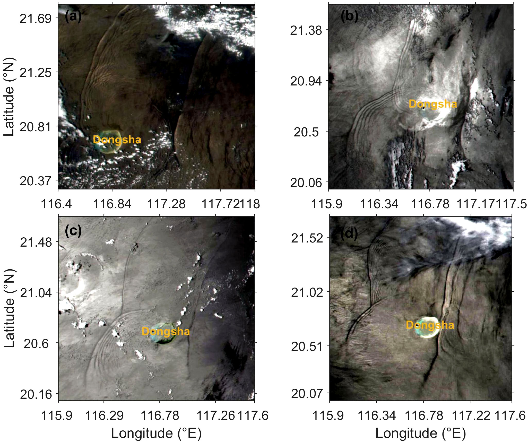
Figure 1 Satellite images exhibit the phenomenon of wave interactions near Dongsha Island. (A–D) are satellite images on 20 April 2019, 16 May 2020, 24 May 2021, 22 July 2021, respectively.
In recent years, more and more studies have begun to focus on the interactions between ISWs and these studies mostly rely on theoretical analysis or satellite images. For example, Hsu and Liu (2000) analyse several hundred satellite images from 1993 to 1999 and find that ISWs occur complex wave-wave interactions after refraction by the topography on the west of Dongsha Island, and one of the obvious features is the phase shift and wavelength change after wave-wave interactions. Chen et al. (2011) find that oblique wave-wave interactions between two ISWs can induce a third ISW through satellite remote sensing images of the South China Sea, and further use the ‘quasi-3D’ Kadomtsev-Petviashvili (KP) equation to provide an explanation on this phenomenon. Differences in the initial amplitude and angle of the incident wave lead to different evolutionary paths and amplitude distributions of the wave-wave interactions, which theoretically predicts the possibility of ‘Mach stem’ (the amplitude of which can be up to four times of the initial amplitude, reflecting the characteristic of a strong nonlinearity) in a typical oceanic background, and emphasises the modulation of the shallow topography (Yuan and Wang, 2022). Elevated amplitudes have a significant impact on the biology of the oceans as well as on the use of industrial technologies such as oil drilling platforms.
Internal waves contain huge amount of energy, derived from tides, surface winds and geostrophic circulation (Egbert and Ray, 2000). ISWs are an important medium for the propagation of energy and momentum in the upper and deeper oceans. Resonance occurs between the ISWs in the oblique wave-wave interactions and their structural stability is weakened. The energy stored in the ISWs is transferred to smaller scale motions, and is eventually dissipated through turbulence (Whalen et al., 2020). Breaking and dissipation are the final stage of the evolution of internal waves, as well as the process of turbulence generation and energy dissipation of conversion of mechanical energy into internal energy, accompanied by enhanced mixing. There are some articles that study mixing caused by internal waves (Xu et al., 2012; Chang et al., 2021). Mixing breaks up the stable stratification of the ocean and triggers the transport of water, heat, nutrients, etc. in the ocean, which is critical to the global energy cycle and the survival of marine organisms (Caldwell and Mourn, 1995). Mixing caused by internal waves can control the processes and outcomes of climate and is also an important link in the energy cycle (Whalen et al., 2020). Shear instability and convective instability is an important generation mechanism of mixing, which can be measured by the Richardson number (Ri). When Ri< 1/4, shear instability dominates, 1/4< Ri< 1, both shear and convective instabilities contribute to enhanced mixing, while Ri > 1, convective instability dominates (Chang, 2021; Ivey et al., 2021; Mashayek et al., 2022). Despite the significance of mixing for ocean circulation, few studies have investigated the relationship between mixing and wave-wave interactions.
Early studies on the oblique wave-wave interactions of ISWs in the South China Sea are mostly based on numerical analyses and summaries of patterns from satellite remote sensing images (Cai and Xie, 2010; Yuan et al., 2018; Yuan et al., 2023). Although there are few systematic studies of wave-wave interactions in the South China Sea under realistic oceanic environment, the related work has been carried out in other seas. For example, Shimizu and Nakayama (2017) used the MITgcm (Massachusetts Institute of Technology General Circulation Model) ocean model results to study the oblique wave-wave interactions between ISWs in the Andaman Sea, and consider the influence of the Coriolis effect caused by the rotation of the Earth. The research aim of this paper is to use the three-dimensional MITgcm model to investigate the oblique wave-wave interactions between ISWs in the northern South China Sea (near Dongsha Island) under realistic ocean conditions, and the impact of this nonlinear interactions on energy dissipation and mixing.
The rest of the paper is organised as follows: Section 2 describes the model setup and theoretical methods, while Section 3 presents the results, including the validation of the model, the variation of waveforms and amplitudes, energy transfer between the first and second modes, as well as the impact on energy dissipation and mixing during wave-wave interactions. Finally, we discuss and conclude in Section 4.
2 Methodology
2.1 Model setup
The South China Sea is known as one of the areas where internal waves are widespread and most of them are caused by tides. In order to study the oblique wave-wave interactions and their impacts in the South China Sea, we carry out a three-dimensional high-resolution simulation of the South China Sea using the MITgcm model, which uses the non-hydrostatic approximation. The simulated area is 115°E-122.5°E, 17.7°N-22.4°N (Figure 2). We use a Cartesian coordinate system in the horizontal directions and z-coordinate in the vertical direction. Since the propagation direction of internal waves in the northern South China Sea is mostly westward or north-westward (Guo et al., 2021) and save resources as much as possible on the basis of satisfying the accuracy, the grid resolution is set to be 500m in the x-direction (East-West direction) and 1000m in the y-direction (North-South direction). In the vertical direction, we use non-uniform grids with a dense grids in the upper ocean and sparse grids in the deep ocean. There are 147 layers in the vertical direction, and the total water depth of the model is set to be 5200m. The layer depth gradually transitions from 1m near the surface to 300m near the bottom. The total number of grid points is 1485×504×147. The topographic data is selected from the GEBCO2020 dataset with a resolution of 1/120°×1/120° (Figure 2), which is interpolated onto the selected grid. To ensure the stability of the model, the minimum water depth of the model is set to 10 m. The viscosity coefficients in the horizontal and vertical directions are uniformly 1.0×10⁻³ m2/s and 1.0×10⁻⁶ m2/s, respectively. The Nonlocal K-Profile Parameterization (KPP) scheme of Large et al. (1994) is used for vertical mixing.
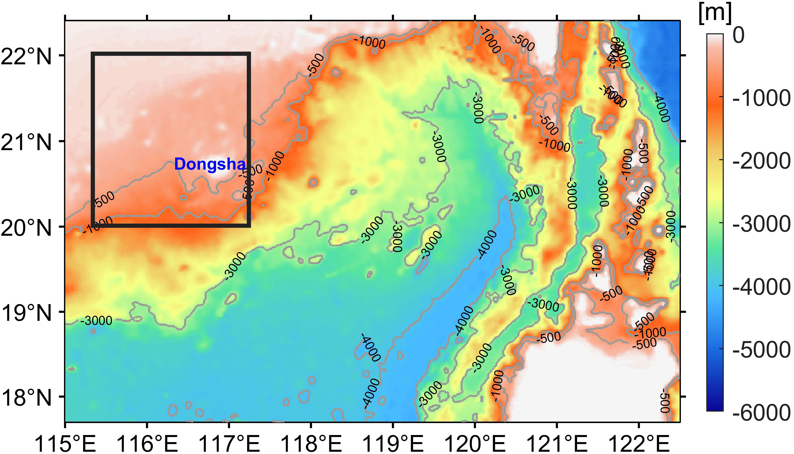
Figure 2 The topography of the simulated area, in which the dark rectangular frame is the major region to study the oblique wave-wave interactions.
Based on Huang et al. (2008), the generation of ISWs exhibits seasonal variation with more occurrences in the northern South China Sea during summer. This is due to the stronger vertical stratification in summer, which favors the westward propagation of the internal waves in the Luzon Strait. So we choose to simulate the South China Sea from 13 May to 29 May 2021. Temperature and salinity data are selected from the World Ocean Atlas 2018 (WOA18) dataset and set to be horizontally homogeneous in the model. Since the monthly averaged data provided in this dataset are limited to the above 1500m of the ocean, in the upper 1500m, we choose the monthly averaged data for May, and we use the seasonal average data below 1500m. The initial temperature and salinity data are shown in Figure 3. Based on the initial temperature and salinity data, the buoyancy frequency is further calculated, where ρ refers to density and can be obtained from the density equation of seawater and z is the vertical coordinate pointing upwards, represents the average density in the vertical direction and g is the gravity acceleration choosing to be 9.8m/s2 here. Since the internal waves in the South China Sea are mostly tide-induced, eight constituents of barotropic tides (M2, S2, N2, K2, K1, O1, P1, and Q1) are selected to drive the model at the four boundaries and the data are derived from the Oregon State University TOPEX/Poseidon Solution (TPXO8-atlas data). In order to avoid the reflection of internal waves affecting the experimental results, we set 20 layers of sponge boundary layer on each of the four boundaries, with the thickness of 10 km in the East-West direction and 20 km in the North-South direction.
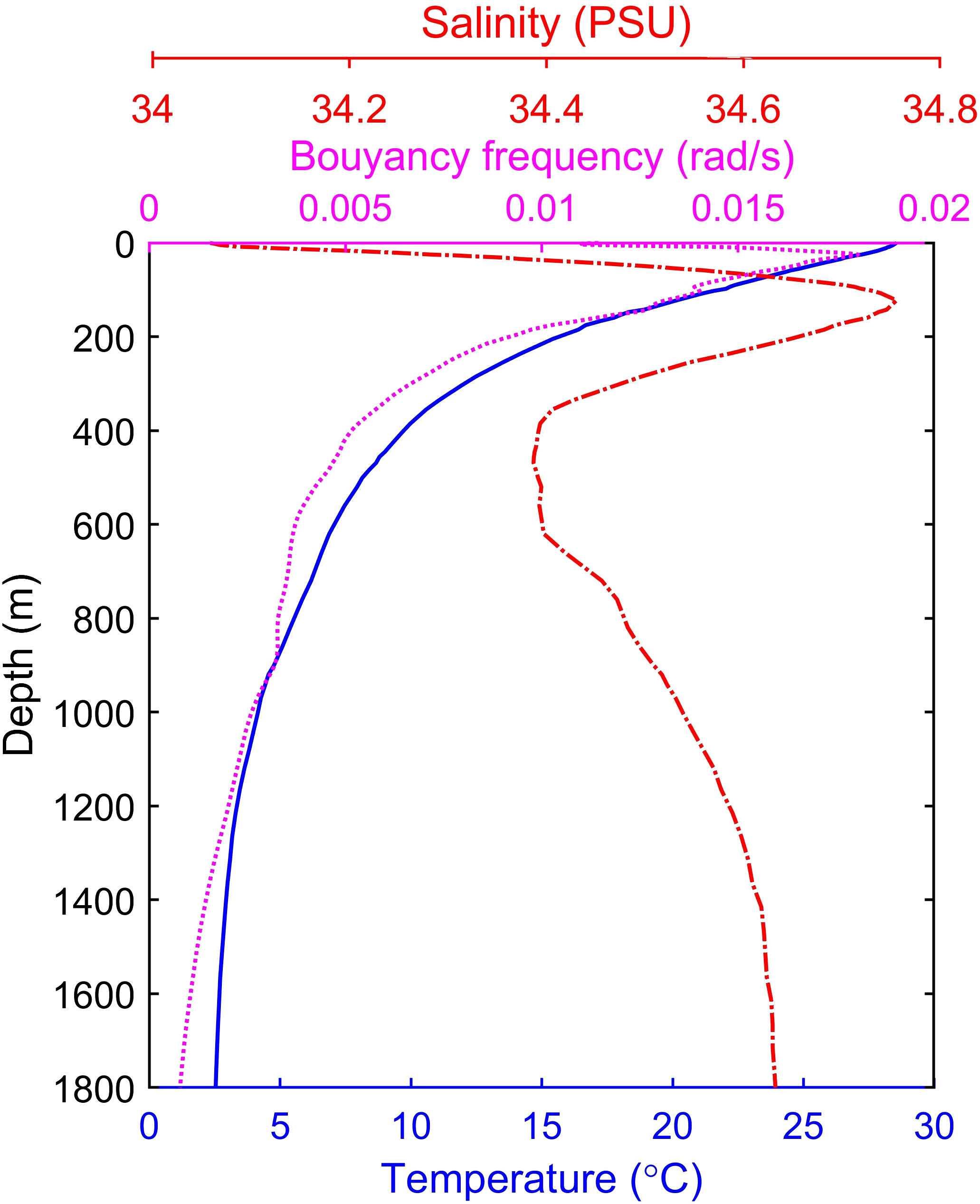
Figure 3 Vertical profiles of initial temperature, salinity, and buoyancy frequency in the simulated region. The blue solid line, red dashed line, and purple dotted line represents temperature, salinity, and buoyancy frequency, respectively.
2.2 Theoretical methods
The theory of oblique wave-wave interactions focuses on the amplitude of two incident waves as well as their intersection regions. So in order to study the oblique internal solitary wave-wave interactions in the South China Sea, the variations of amplitudes are important. According to Yuan et al. (2018), considering the Boussinesq approximation and rigid lid approximation in oceanography, when the background flow is absent, we can obtain the amplitude based on the temperature, salinity, and velocity data output by the model where the subscript n represents the mode number, for example, n = 1 represents mode-1 waves while n = 2 mode-2 waves. Λn,cn,ϕn represent the amplitude, phase speed, mode function of a fixed mode, respectively. h,u are the water depth and particle velocity along the wave propagation direction, respectively. z is the vertical coordinate pointing upwards. cn and ϕn can be obtained by solving the following modal equation
where the subscript z represents a second-order derivatives with respect to z. The Boussinesq approximation is again applied and since the modal function is orthogonal to the weighting function N2, the domain integrated available potential energy (APE) for each mode is
where Pn represents the potential energy of different modes and the ρ0 is background density field. The domain-integrated kinetic energy (KE) for each mode simplifies to
where un and wn are velocity components in each internal wave mode. As in the long-wave limit used here un >> wn. So the total energy for each mode is En = 2Kn = 2Pn. Note that Equations (3, 4) are based on the assumption of inviscid and frictionless fluid, thus the effects of bottom friction and viscosity are ignored.
In stratified oceans, the Osborn model can be used to quantify turbulent mixing rate (Osborn, 1980),
where Kρ,N,ϵ,γ represent the mixing rate, buoyancy frequency, turbulent kinetic energy dissipation rate and mixing coefficient, respectively. Many studies have shown that the mixing coefficient γ will change with marine environment. Based on the in-situ observation in the South China Sea (Lu et al., 2009), γ = 0.11 is used in this article. Then the turbulent kinetic energy dissipation rate ϵ with velocity shears can be given by
where u and v represent the eastward and northward components of the velocity field, respectively. S represents the vertical velocity shear and ν is the kinematic viscosity of seawater, which is taken as 10−6m2/s here. In addition, the Ri can quantify and judge the mechanism of mixing and can be defined by
3 Results
3.1 Model validation
3.1.1 Barotropic tidal validation
To validate the model, we set up a standard experiment with a homogeneous temperature and salinity field across the field (initial temperature set to 5°C and salinity to 34 psu) using hydrostatic approximation. The simulation duration increases to 120 days and other conditions keep consistent with the experiments mentioned in Section 2.1. Based on the output results of the standard experiment, we select the fluctuations of sea surface from day 16 to day 120 and carry out harmonic analysis using the T-Tide toolkit to obtain the amplitude and phase of tidal components, then compare them with the corresponding amplitude and phase from the TPXO8 dataset. As the M2 and K1 components are relatively powerful among all tidal constituents (Guo and Chen, 2014), we show the comparison of M2 and K1 components between the model results and TPXO8 data.The comparison results are shown in Figure 4, where the cotidal chart of semidiurnal tide M2 from the MITgcm model is generally consistent with that from TPXO8 in terms of amplitude. However, there is a slight difference in the comparison of the amplitude of K1, which is slightly larger obtained from the model. It may be due to the fact that the bathymetry and resolution used by the model are different from TPXO8. The phases of M2 and K1 obtained from the model are the same as that of TPXO8. Overall, the results simulated by the model are basically consistent with TPXO8, indicating the validity of model.
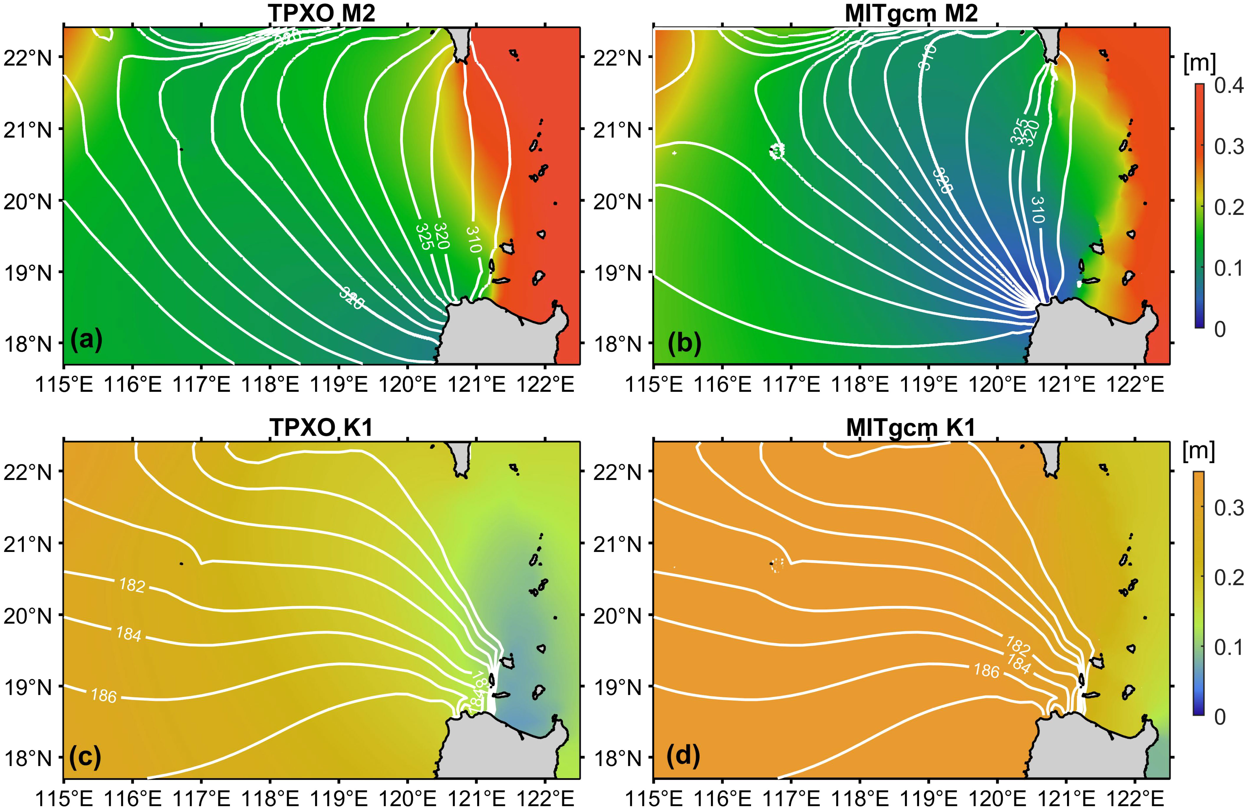
Figure 4 Cotidal chart for M2 and K1 in the simulated area based on TPXO (A, C) and MITgcm (B, D) results, where the colors indicate the amplitude and white solid lines represent the phase.
3.1.2 Satellite image validation
The ISWs can cause the sea surface to converge or diverge, so as to adjust the roughness of the sea surface, which can be recognised as alternating dark and bright ripples on the satellite images. So the basic information of ISWs can be obtained from the satellite images (Liu et al., 1998). Therefore, we can validate the model from the two-dimensional perspective by comparing the satellite data with the model results. Sea surface height gradient (SSHG) can portray the spatial position of internal waves in two-dimensional perspective, and the formula for SSHG is
where ζ is the sea surface height (with respect to the stationary sea surface as the origin and upward as the positive direction). Based on the results output by the model, it is easy to calculate SSHG (Equation 9) at different moments. In this article, the horizontal distributions of SSHG on 19 May 2021 are selected to show the consistency with the satellite images in Figure 5.
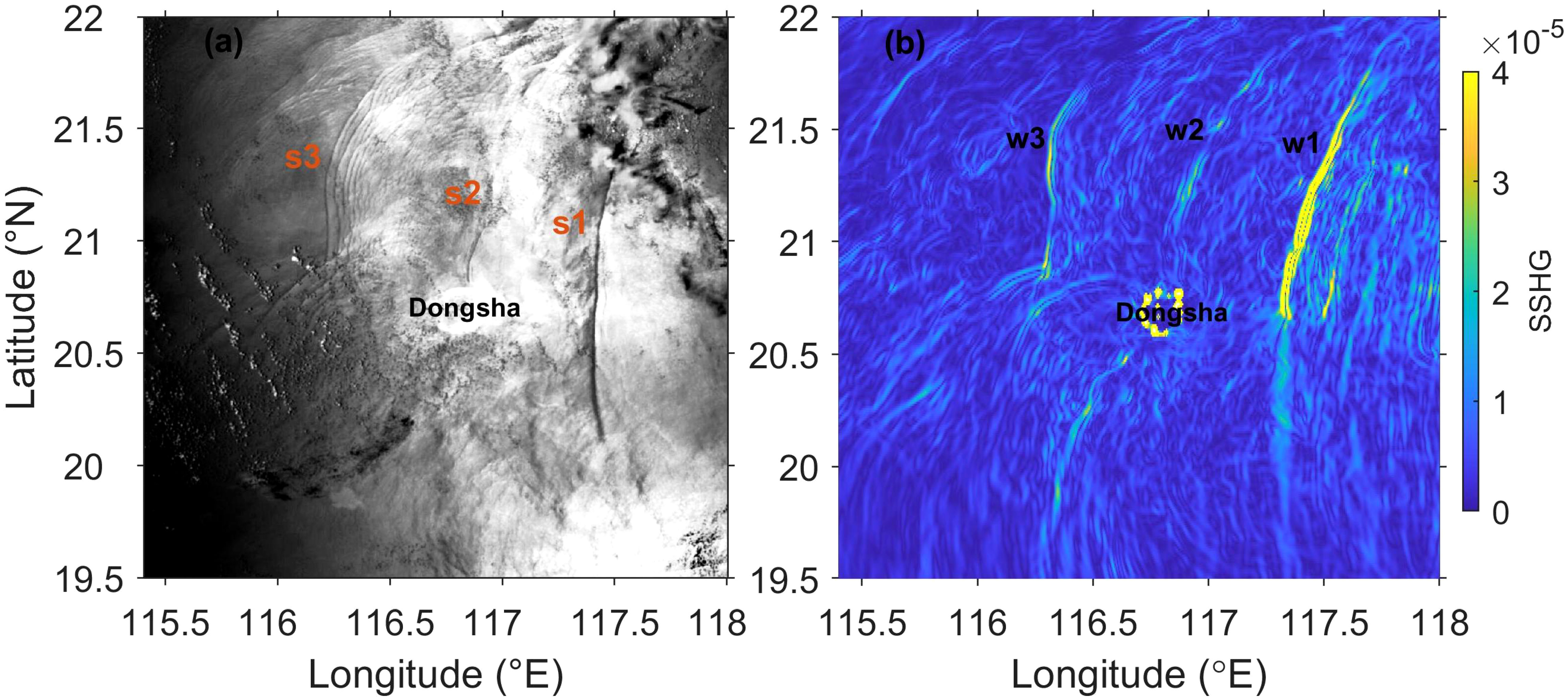
Figure 5 (A) shows a satellite image (Dongsha Island marked in black label) and (B) shows the distribution of SSHG on 19 May 2021. s1,s2,s3 are three ISWs at different locations in (A) and w1, w2, w3 are three ISWs in (B).
According to Figure 5B, there are three relatively large ISWs labeled as w1, w2 and w3 between 116°E and 117.5°E. The first one is located around 117.4°E labeled as w1, which corresponds to the white line on the satellite image around 117.4°E labeled as s1. There is a slight error. The value of SSHG on the south side of wave crest line (about south of 20.7°N) decreases, while a clear white line exists at the same position in the satellite image. The second one is the wave field located on the north and south sides of Dongsha Island labeled as w2, corresponding to the white line on the north side of Dongsha Island in the satellite image labeled as s2. The third one is a crossed X-shaped wave train located on the west side of Dongsha Island (around 116.2°E) labeled as w3, corresponding to the intersecting white lines around 116.2°E in the satellite image labeled as s3. Compared with the real ocean, the MITgcm model lacks factors such as background circulation in our work, so the model results differ slightly from satellite image. The model results are in good agreement with the satellite images in general, which indicates the validity of the model.
3.2 Variation of amplitude and energy
Most of the ISWs in the northern South China Sea originate from the Luzon Strait. During the westward propagation of ISWs, they may encounter the continental shelf and other shallow water terrains such as the Dongsha Island. Due to the change of environmental factors such as depth, stratification etc., the reflection and diffraction of ISWs occur, resulting in complex intersection between wave crest lines. Although the oblique intersection between ISWs is complex in the northern South China Sea, which makes it difficult to study the oblique wave-wave interactions between two undisturbed ISWs, we find a prominent ISWs interaction near the west side of Dongsha Island (116.23°E, 20.64°N) based on model results. The intensity of this wave is large, which makes the interference of other internal waves with this crossed ISW relatively small. In order to study the propagation process of the above mentioned crossed wave, we plot the distribution diagrams of SSHG at different moments based on the model output, and put several typical moments together to observe the evolution of this ISWs more intuitively.
The westward propagating ISW in the northern South China Sea diffracts when passing Dongsha Island at time 188h. After diffraction, the ISW begins to cross at 116.59°E (Figure 6A), and the crossed ISW continues to propagate westward (Figure 6B). We can see that the value of the SSHG in the centre of the crossed point increases during propagation (Figure 6C), and then the ISW maintains this pattern and gradually shifts to the southwest. In the final stage of propagation, the energy cannot maintain the existing state of ISW, which gradually breaks up until it disappears due to the dissipation and bottom friction (Figure 6D). From the figure of the ISW evolution, we can observe that the value of the crossed section of this ISW is increasing, these two leading waves render the oblique wave-wave interactions.
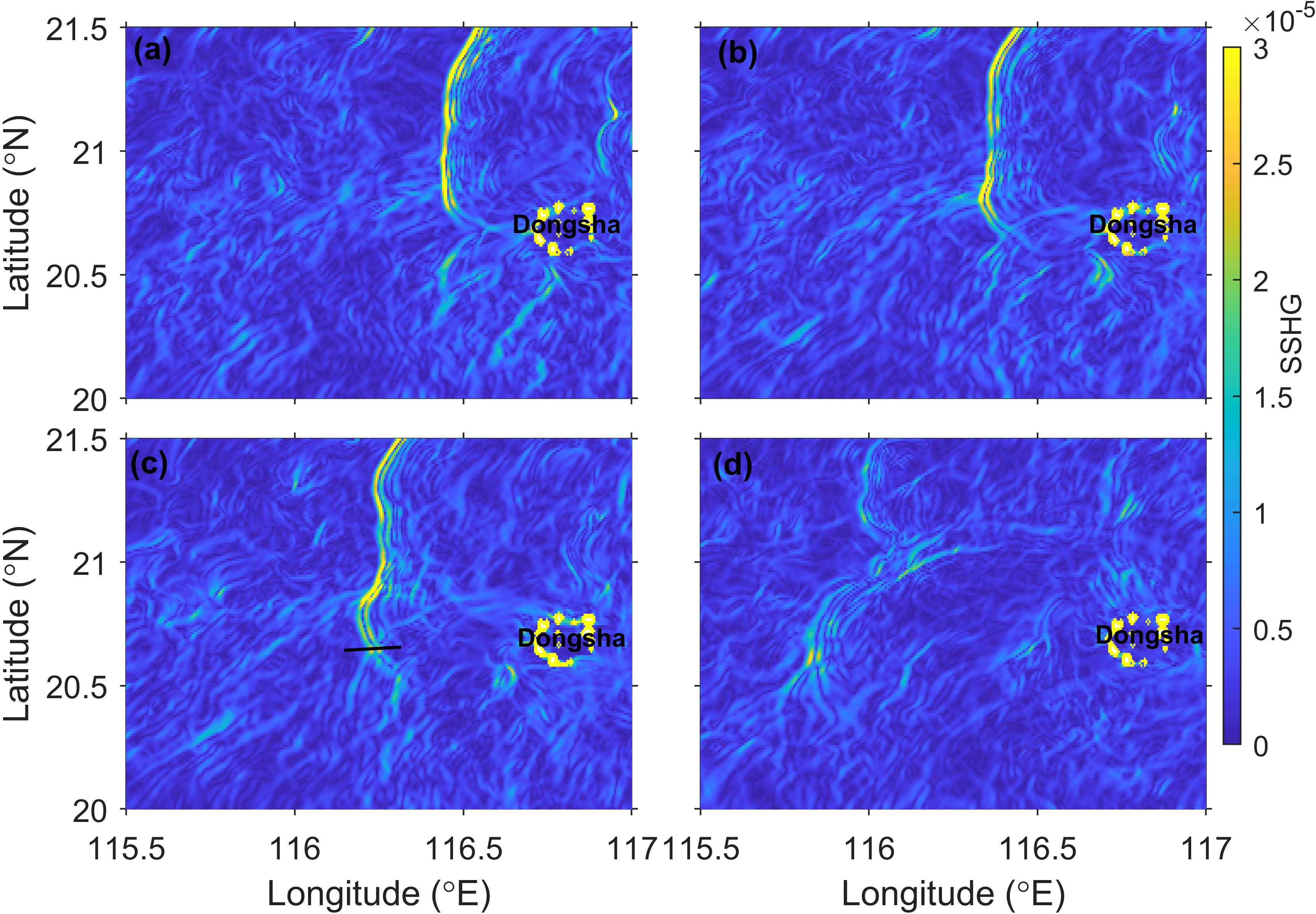
Figure 6 (A–D) show the distribution of SSHG at time 198h, 200h, 202.5h and 209h, respectively. The position of the dark solid line in (C) is the profile for calculating the amplitude of the crossed ISW, energy dissipation rate, mixing rate and Richardson number at time 202.5h.
The distribution of SSHG is mainly the result of ocean surface fluctuations, which can only indirectly reflect the variations in the vertical structure of ISWs within the ocean interior, while the oblique wave-wave interactions theory focuses on the amplitude changes in the wave crossed section. In order to better reveal the variations of the amplitude, we calculate the amplitude of the central region of the crossed section. The whole oblique interactions between ISWs lasts for 11h. Firstly, a suitable section is determined based on the wave direction at each moment, then we calculate the amplitude on the section at each moment (with a time interval of 30 minutes) using the temperature, salinity, and particle velocity output by the model and plot the amplitude change curve based on Equation (1) (Figure 7).
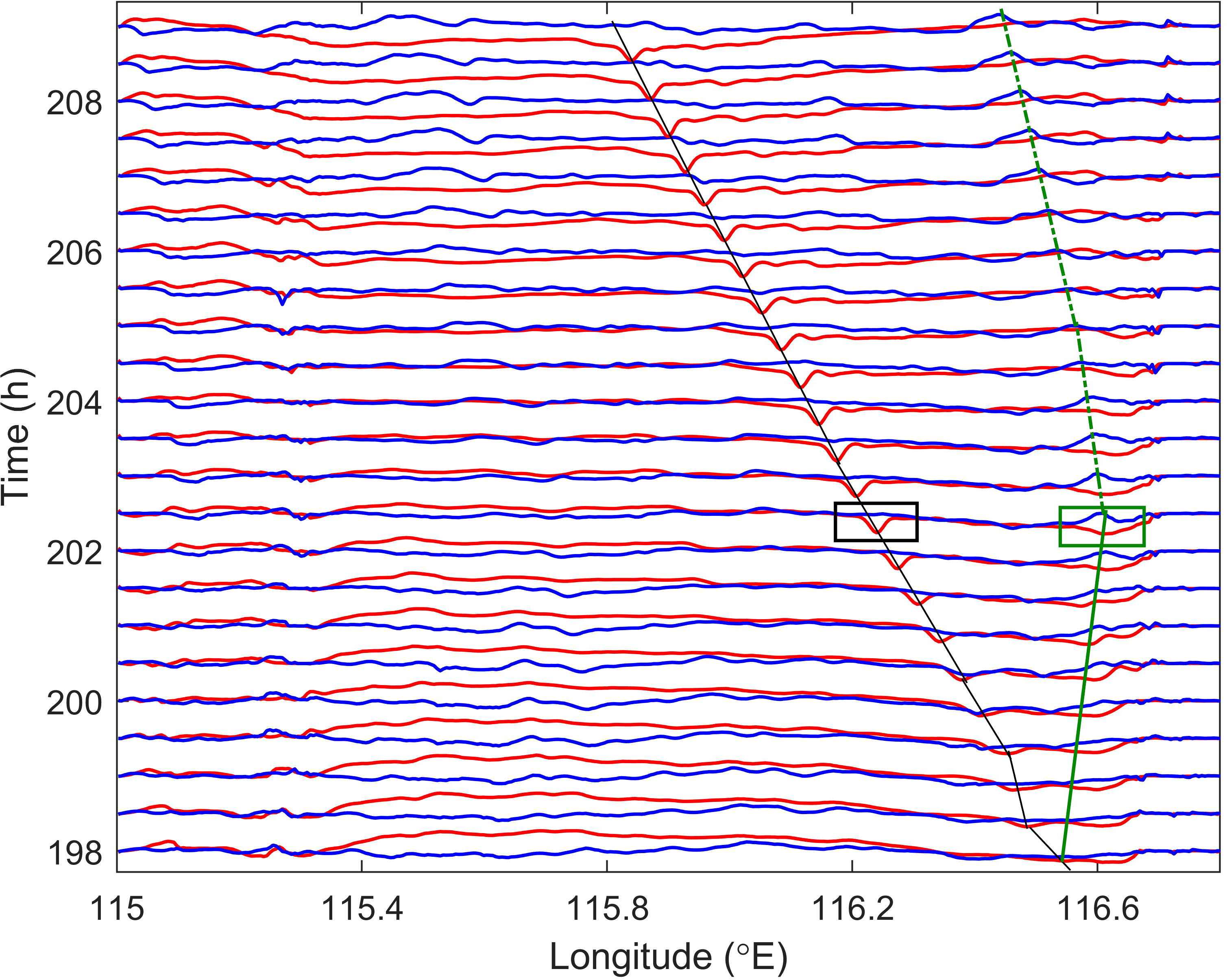
Figure 7 Time series of amplitude along the intersection line as shown in Figure 6. The red and blue solid lines are the amplitude of the first and second mode, respectively. The black and green solid lines represent the propagation paths of the first mode and second mode waves, respectively, while the green dashed line represents the propagation path of the second mode wave after being reflected by Dongsha Island. The black and green rectangles represent the areas that are selected for calculating the energy of the first and second mode waves, respectively.
Wave-wave interactions occur after the ISWs cross, and as can be seen from Figure 7, mode transformation and waveform changes take place during this nonlinear interactions. The main wave of the first mode continues to propagate westward, while the main wave of the second mode propagates in the opposite direction to the first mode after its generation. The second mode main wave is reflected when encounter the obstruction of Dongsha Island in the process of propagation, and then it shifs to propagate westward. In order to validate the accuracy of main wave of the first and second mode, we calculate the theoretical phase speed and numerical phase speed by Equation (2) through modal decomposition and their locations at different moments, respectively. And then we compare two kinds of speed (Figure 8). During the initial stage of wave-wave interactions, there is a significant difference between theoretical speed and numerical speed, especially for the first mode. This could be attributed to that Equation (2) used to calculate the theoretical phase speed is an reduction of the primary Navier-Stokes equations, which leads to differences between the theories and numerical results. Though the differences still exist in the later stage of wave-wave interactions, the agreement between the theoretical and numerical values is relatively better compared to the earlier stage.
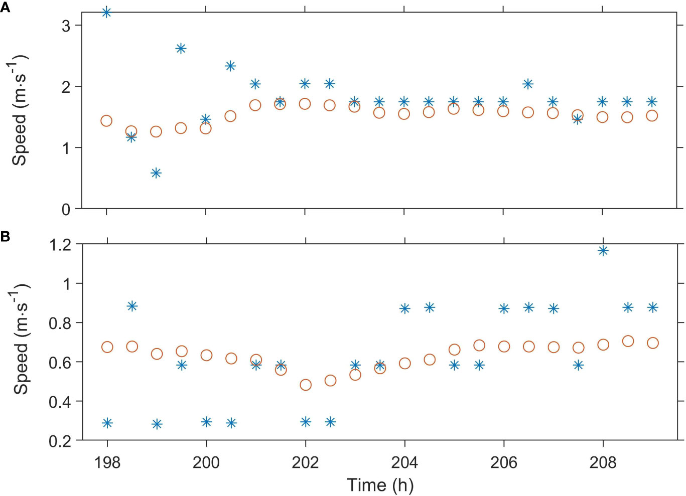
Figure 8 (A, B) represent the variations of phase speed of the first and second mode wave, respectively. The red circles represent the theoretical phase speed of the first and second mode wave, and the blue asterisks represent the numerical speed of the first and second mode wave.
The amplitudes of ISWs are closely related to their energy. Therefore, we calculate the energy of the first and second mode main waves at different times using Equations (3, 4) (Figure 9). The black and green rectangles in Figure 7 indicate the regions where the energy of the main waves is calculated. The positions of the two rectangles change with the variation of the main wave positions at different monments, but the sizes of rectangles remain constant. It can be observed that the energy of the first mode main wave is basically in the trend of first increasing and then decreasing, see Figure 9. The nonlinear enhancement leads to an increase in the amplitude of intersection region at the beginning of the wave-wave interactions and the energy also grows. As the nonlinear interactions progresses, the energy of the first mode is converted to the second mode, and the energy is also dissipated due to bottom friction and viscosity. Therefore, after time t = 202h, overall, the energy of the first mode is in a trend of decreasing. The energy of the second mode main wave also generally follows a trend of initially increasing and then decreasing. Due to the wave-wave interactions, the energy of the first mode is converted to the second mode, resulting in an increase in the energy of the second mode. However, during the propagation of the second mode main wave, energy is dissipated on account of bottom friction and other factors, leading to the continuous decrease in energy.
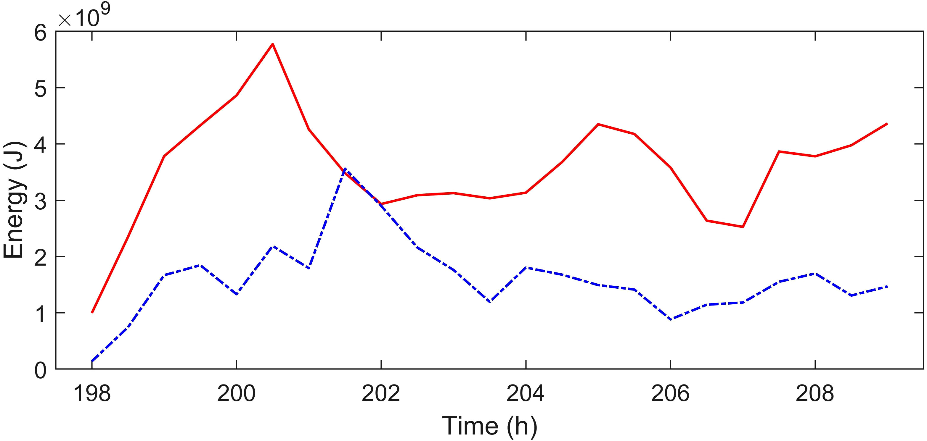
Figure 9 Energy variations of the first and second mode main waves. The red solid line and the blue dashed line represent the energy of the first and second mode main waves, respectively.
3.3 The increase of energy dissipation rate and mixing rate
Mixing in marginal seas plays an important role in global ocean circulation and heat transport. The South China Sea is one of the largest marginal seas in the Pacific Ocean, characterised by complex seabed topography and strong tidal currents. Turbulent mixing is also one of the main pathways for energy transport in the global ocean. The crossed ISW propagates to around 116.24°E at time 202.5h. The profile (marked by the solid black line in Figure 7C) at 20.64°N is selected, and the turbulent kinetic energy dissipation rate, mixing rate, Ri are calculated on this profile at time 202.5h through Equations (5–8) (Figure 10).
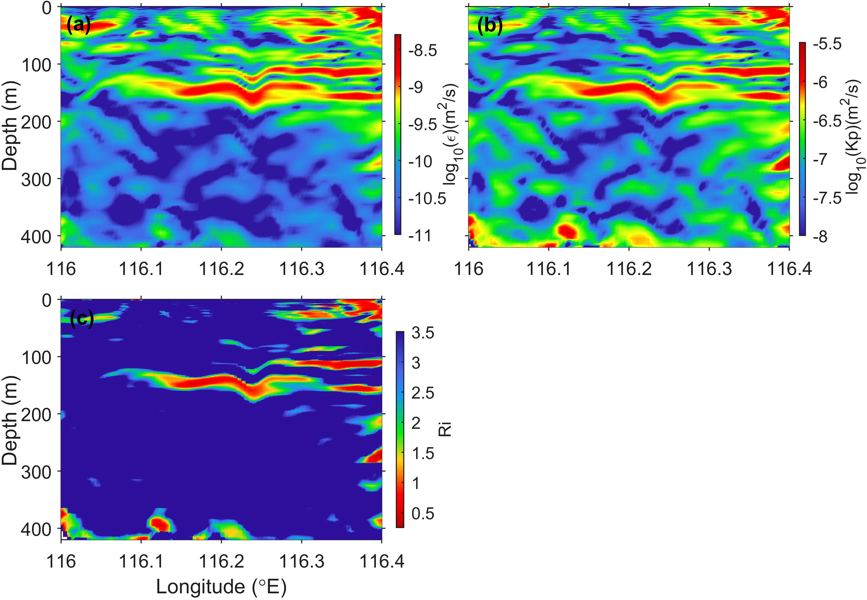
Figure 10 (A–C) show the variation of energy dissipation rate, mixing rate and Richardson number of the 20.64°N profile at time 202.5h, respectively.
By means of Figure 10A, it can be seen that the turbulent kinetic energy dissipation rate in certain areas near 116.24°E is significantly enhanced compared to the surrounding regions, with an increase of approximately one to two orders of magnitude. The increase of turbulent kinetic energy dissipation rate may be caused by the following reasons: Firstly, based on two-dimensional distribution of SSHG, it is noted that the wave is propagating near 116.24°E at time 202.5h. Consequently, some of the energy is dissipated by the bottom friction, which leads to an increase in the dissipation rate. Secondly, it is found that there existes the generation of the second mode ISW in the process of wave-wave interactions by observing the change of amplitude. The amplitude is closely related to the energy variation, so another part of the energy is converted into higher mode ISW. However, due to the highly unstable structure of the high mode ISW, it is prone to be unstable, leading to an increase in the local dissipation rate.
Internal waves inherently contain a huge amount of energy. The interactions between ISWs and steep topography or between the ISWs can transfer their energy into small scale motions (Garrett and St. Laurent, 2002). Eventually, these waves break up and generate turbulence, leading to an increase in mixing rate. We investigate the mixing rate on the 20.64°N profile at time 202.5h (Figure 10B). It is found that there is an obvious increase in the mixing rate around 116.24°E, and different peaks of mixing rate enhancement occur at different depths. At time 202.5h, the ISW propagates near 116.24°E. Because the nonlinear interactions occurs during the propagation of ISWs, which leads to nonlinear enhancement. When the nonlinear enhancement reaches a certain level, it will cause the internal wave field unstable and then the vertical shear instability enhances. According to previous studies (Vlasenko and Hutter, 2002; Lamb, 2003), both shear instability and convective instability are important factors contributing to the increase in mixing rate. The relationship between shear instability and convective instability is complex. The Ri on the profile 20.64°N is calculated at time 202.5h in this article (Figure 10C). Ri is found to be roughly 0.25 < Ri < 1 in regions of elevated mixing rates, which suggests that the enhanced mixing is the result of both shear instability and convective instability. In addition, it is also possible that high mode ISW generate during the wave-wave interactions, but the structure of high mode ISW is prone to be unstable, which ultimately leads to higher mixing rates.
4 Discussion and conclusions
A high-resolution three-dimensional MITgcm model is used to investigate the oblique wave-wave interactions between ISWs in the South China Sea (near Dongsha Island) in this article. The findings regarding the wave-wave interactions and their impact on energy dissipation and mixing are discussed on the west side of Dongsha Island. Furthermore, the mechanism of mixing rate enhancement is also explored. Firstly, SSHG is calculated based on the model results at each moment and it is observed that a large number of crossed ISWs exist near the Dongsha Island. And according to previous studies, a considerable number of remote sensing satellite images have captured the phenomena of wave crest line intersection near Dongsha Island, which all indicates the occurrence of wave-wave interactions.
A prominent crossed ISW emerge on the west side of Dongsha Island without any other strong waves in its periphery. The amplitude of this ISW is calculated using the temperature and salinity output by the model. The calculation results show that mode transformation and waveform changes occur in the whole process of wave-wave interactions. To verify the precision of the first and second mode main waves, we calculate the theoretical and numerical phase speeds of the two main waves using mode decomposition and their locations at different times. In the initial stage of wave-wave interactions, there is a significant difference between the theoretical and numerical phase speeds. However, in the later stage of wave-wave interactions, although some differences still persisted, the agreement between them improved compared to the earlier stage. In addition, we also calculate the energy of main wave of the first and second mode, and the analysis reveals that the energy of these two modes exhibits a general trend of initially increasing and then decreasing over time. The increase in the amplitude of first mode is attributed to the enhancement of nonlinear and the energy of ISWs is closely related to the amplitude, so the energy of the first mode is constantly increasing. Because of the mode transformation during wave-wave interactions, the energy of the first mode is converted to the second mode, resulting in a decrease in the energy of first mode and an increase in the energy of second mode. Furthermore, the energy of first mode and second mode tends to decrease eventually due to dissipation partly caused by bottom friction.
We calculate the energy dissipation rate, mixing rate, and Ri on the profile 20.64°N at time 202.5h and find that both the energy dissipation rate and mixing rate increase around 116.24°E. The increase in dissipation rate is consistent with the occurrence of ISWs’ oblique interactions. Additionally, the wave-wave interactions causes that the energy of the first mode is converted into higher mode ISW. However, these higher mode ISW has unstable structures and are prone to breaking, leading to the increase in energy dissipation rate and mixing rates. When the oblique wave-wave interactions occur, the nonlinearity is enhanced and the amplitude is augmented, causing the internal wave field to become unstable, as suggested by the mixing rate and Ri. The results reveal that the region where mixing rate increase corresponds to 1/4< Ri< 1. Therefore, both shear instability and convective instability contribute to the increase in mixing rates.
In conclusion, the three-dimensional numerical model is used to simulate the oblique internal solitary wave-wave interactions in this work, which expands the understanding of wave-wave interactions in realistic ocean. In addition, this study further elaborates the impact of wave-wave interactions on mixing. Note that mixing can lead to the transport of nutrients in the vertical direction and indeed, Wu et al. (2023) showed that the asymmetric distribution of chlorophyll-a near the Dongsha Atoll is enhanced by internal waves, which suggests the potential importance of internal wave-wave interactions on biological processes. Nevertheless, this work still leaves some problems to be solved further. Here the conclusions are based on the numerical simulations and if available, the in-situ observational data would provide deep insights to verify the conclusions in this paper. More importantly, the region considered in this paper is not large enough to incorporate the shallow region of the Western South China Sea, where abounds small-scale topographic features and it has a possibility to generate internal solitary waves (Bai et al., 2023) intermittently, which means internal solitary wave-wave interactions could also frequently occur in this region, which would be of interest to do further study.
Data availability statement
The original contributions presented in the study are included in the article/supplementary materials, further inquiries can be directed to the corresponding author.
Author contributions
YJ: Data curation, Software, Visualization, Writing – original draft. YG: Data curation, Resources, Validation, Writing – review & editing. ZZ: Conceptualization, Data curation, Formal analysis, Resources, Validation, Writing – review & editing. CY: Conceptualization, Funding acquisition, Methodology, Supervision, Writing – review & editing. PZ: Writing – review & editing.
Funding
The author(s) declare financial support was received for the research, authorship, and/or publication of this article. This work was supported by the National Natural Science Foundation of China (Nos. 42006016, 42006154), the Fundamental Research Funds for the Central Universities (202265005, 202264007), the key program of the National Natural Science Foundation of China (91958206), the State Key Laboratory of Tropical Oceanography, South China Sea Institute of Oceanology, Chinese Academy of Sciences (Project No. LTO2303), the Natural Science Foundation of Shandong Province (ZR2020QD063).
Acknowledgments
The authors would like to thank the reviewers for their valuable suggestions on the manuscript.
Conflict of interest
The authors declare that the research was conducted in the absence of any commercial or financial relationships that could be construed as a potential conflict of interest.
Publisher’s note
All claims expressed in this article are solely those of the authors and do not necessarily represent those of their affiliated organizations, or those of the publisher, the editors and the reviewers. Any product that may be evaluated in this article, or claim that may be made by its manufacturer, is not guaranteed or endorsed by the publisher.
References
Bai X., Lamb K. G., Liu Z., Hu J. (2023). Intermittent generation of internal solitary-like waves on the Northern shelf of the South China Sea. Geophysical Res. Lett. 50, e2022GL102502. doi: 10.1029/2022GL102502
Cai S., Xie J. (2010). A propagation model for the internal solitary waves in the Northern South China Sea. J. Geophysical Res. 115, C12074. doi: 10.1029/2010JC006341
Caldwell D. R., Mourn J. N. (1995). Turbulence and mixing in the ocean. Rev. Geophysics 33, 1385–1394. doi: 10.1029/95RG00123
Chang M.-H. (2021). Marginal instability within internal solitary waves. Geophysical Res. Lett. 48, e2021GL092616. doi: 10.1029/2021GL092616
Chang M., Cheng Y., Yang Y. J., Jan S., Ramp S. R., Reeder D. B., et al. (2021). Direct measurements reveal instabilities and turbulence within large amplitude internal solitary waves beneath the ocean. Commun. Earth Environ. 2, 15. doi: 10.1038/s43247-020-00083-6
Chao S.-Y., Shaw P.-T., Hsu M.-K., Yang Y.-J. (2006). Reflection and diffraction of internal solitary waves by a circular island. J. Oceanogr. 62, 811–823. doi: 10.1007/s10872-006-0100-4
Chen G.-Y., Liu C.-T., Wang Y.-H., Hsu M.-K. (2011). Interaction and generation of long-crested internal solitary waves in the South China Sea. J. Geophysical Res.: Oceans 116, C06013. doi: 10.1029/2010JC006392
Du T., Tseng Y.-H., Yan X.-H. (2008). Impacts of tidal currents and kuroshio intrusion on the generation of nonlinear internal waves in Luzon strait. J. Geophysical Res. 113, C08015. doi: 10.1029/2007JC004294
Egbert G. D., Ray R. D. (2000). Significant dissipation of tidal energy in the deep ocean inferred from satellite altimeter data. Nature 405, 775–778. doi: 10.1038/35015531
Garrett C., St. Laurent L. (2002). Aspects of deep ocean mixing. J. Oceanogr. 58, 11–24. doi: 10.1023/A:1015816515476
Guo Z., Cao A., Wang S. (2021). Influence of remote internal tides on the locally generated internal tides upon the continental slope in the South China Sea. J. Mar. Sci. Eng. 9, 1268. doi: 10.3390/jmse9111268
Guo C., Chen X. (2014). A review of internal solitary wave dynamics in the Northern South China Sea. Prog. Oceanogr. 121, 7–23. doi: 10.1016/j.pocean.2013.04.002
Guo C., Chen X., Vlasenko V., Stashchuk N. (2011). Numerical investigation of internal solitary waves from the Luzon strait: Generation process, mechanism and three-dimensional effects. Ocean Model. 38, 203–216. doi: 10.1016/j.ocemod.2011.03.002
Helfrich K. R., Melville W. K. (2006). Long nonlinear internal waves. Annu. Rev. Fluid Mech. 38, 395–425. doi: 10.1146/annurev.fluid.38.050304.092129
Hsu M.-K., Liu A. K. (2000). Nonlinear internal waves in the South China Sea. Can. J. Remote Sens. 26, 72–81. doi: 10.1080/07038992.2000.10874757
Huang W., Johannessen J., Alpers W., Yang J., Gan X. (2008). “Spatial and temporal variations of internal wave sea surface signatures in the Northern South China Sea studied by spaceborne sar imagery,” in Lacoste H., Ouwehand L editors. Advances in SAR Oceanography from ENVISAT and ERS missions (Frascati, Italy: ESA ESRIN).
Ivey G. N., Bluteau C. E., Gayen B., Jones N. L., Sohail T. (2021). Roles of shear and convection in driving mixing in the ocean. Geophysical Res. Lett. 48, e2020GL089455. doi: 10.1029/2020GL089455
Jia T., Liang J., Li X.-M., Sha J. (2018). Sar observation and numerical simulation of internal solitary wave refraction and reconnection behind the dongsha atoll. J. Geophysical Res.: Oceans 123, 74–89. doi: 10.1002/2017JC013389
Jin G., Lai Z., Shang X. (2021). Numerical study on the spatial and temporal characteristics of nonlinear internal wave energy in the Northern South China Sea. Deep Sea Res. Part I: Oceanographic Res. Pap. 178, 103640. doi: 10.1016/j.dsr.2021.103640
Klymak J. M., Pinkel R., Liu C.-T., Liu A. K., David L. (2006). Prototypical solitons in the South China Sea. Geophysical Res. Lett. 33, L11607. doi: 10.1029/2006GL025932
Lamb K. G. (2003). Shoaling solitary internal waves: on a criterion for the formation of waves with trapped cores. J. Fluid Mechanics 478, 81–100. doi: 10.1017/S0022112002003269
Large W. G., McWilliams J. C., Doney S. C. (1994). Oceanic vertical mixing: A review and a model with a nonlocal boundary layer parameterization. Rev. Geophysics 32, 363–403. doi: 10.1029/94RG01872
Liu A. K., Chang Y. S., Hsu M.-K., Liang N. K. (1998). Evolution of nonlinear internal waves in the East and South China Seas. J. Geophysical Res.: Oceans 103, 7995–8008. doi: 10.1029/97JC01918
Liu C.-T., Pinkel R., Klymak J., Hsu M.-K., Chen H.-W., Villanoy C. (2006). Nonlinear internal waves from the Luzon strait. Eos Trans. Am. Geophysical Union 87, 449–451. doi: 10.1029/2006EO420002
Lu Z., Chen G., Xie X., Xu X., Shang X. (2009). The research of the micro-scale characteristic of the ocean mixing in the Northern South China Sea in the summer. Prog. Nat. Sci. 19, 647–663.
Magalhaes J., Pires A., da Silva J., Buijsman M., Oliveira P. (2021). Using sar imagery to survey internal solitary wave interactions: A case study off the Western Iberian shelf. Continental Shelf Res. 220, 104396. doi: 10.1016/j.csr.2021.104396
Mashayek A., Baker L., Cael B., Caulfield C. (2022). A marginal stability paradigm for shear-induced diapycnal turbulent mixing in the ocean. Geophysical Res. Lett. 49, e2021GL095715. doi: 10.1029/2021GL095715
Osborn T. (1980). Estimates of the local rate of vertical diffusion from dissipation measurements. J. Phys. Oceanogr. 10, 83–89. doi: 10.1175/1520-0485(1980)010<0083:EOTLRO>2.0.CO;2
Ramp S. R., Tang T. Y., Duda T. F., Lynch J. F., Liu A. K., Chiu C.-S., et al. (2004). Internal solitons in the Northeastern South China Sea. part i: Sources and deep water propagation. IEEE J. Oceanic Eng. 29, 1157–1181. doi: 10.1109/JOE.2004.840839
Shimizu K., Nakayama K. (2017). Effects of topography and Earth’s rotation on the oblique interaction of internal solitary-like waves in the Andaman Sea. J. Geophysical Res.: Oceans 122, 7449–7465. doi: 10.1002/2017jc012888
Vlasenko V., Hutter K. (2002). Numerical experiments on the breaking of solitary internal wavesover a slope–shelf topography. J. Phys. Oceanogr. 32, 1779–1793. doi: 10.1175/1520-0485(2002)032<1779:NEOTBO>2.0.CO;2
Wang C., Pawlowicz R. (2012). Oblique wave-wave interactions of nonlinear near-surface internal waves in the strait of Georgia. J. Geophysical Res.: Oceans 117, C06031. doi: 10.1029/2012JC008022
Whalen C. B., De Lavergne C., Naveira Garabato A. C., Klymak J. M., MacKinnon J. A., Sheen K. L. (2020). Internal wave-driven mixing: Governing processes and consequences for climate. Nat. Rev. Earth Environ. 1, 606–621. doi: 10.1038/s43017-020-0097-z
Wu M., Xue H., Chai F. (2023). Asymmetric chlorophyll responses enhanced by internal waves near the Dongsha Atoll in the South China Sea. J. Oceanol. Limnol. 41, 418–426. doi: 10.1007/s00343-022-1434-5
Xu J., Xie J., Chen Z., Cai S., Long X. (2012). Enhanced mixing induced by internal solitary waves in the South China Sea. Continental Shelf Res. 49, 34–43. doi: 10.1016/j.csr.2012.09.010
Xue J., Graber H. C., Romeiser R., Lund B. (2014). Understanding internal wave–wave interaction patterns observed in satellite images of the Mid-atlantic bight. IEEE Trans. Geosci. Remote Sens. 52, 3211–3219. doi: 10.1109/TGRS.2013.2271777
Yuan C., Grimshaw R., Johnson E. (2018). The evolution of second mode internal solitary waves over variable topography. J. Fluid Mechanics 836, 238–259. doi: 10.1017/jfm.2017.812
Yuan C., Pan L., Gao Z., Wang Z. (2023). Combined effect of topography and rotation on oblique internal solitary wave-wave interactions. J. Geophysical Res.: Oceans 128, e2023JC019634. doi: 10.1029/2023JC019634
Yuan C., Wang Z. (2022). On diffraction and oblique interactions of horizontally two-dimensional internal solitary waves. J. Fluid Mechanics 936, A20. doi: 10.1017/jfm.2022.60
Keywords: South China Sea, internal solitary waves, oblique wave-wave interactions, mode transformations, mixing
Citation: Jia Y, Gong Y, Zhang Z, Yuan C and Zheng P (2024) Three-dimensional numerical simulations of oblique internal solitary wave-wave interactions in the South China Sea. Front. Mar. Sci. 10:1292078. doi: 10.3389/fmars.2023.1292078
Received: 10 September 2023; Accepted: 04 December 2023;
Published: 03 January 2024.
Edited by:
Zhiyu Liu, Xiamen University, ChinaReviewed by:
Junde Li, Hohai University, ChinaAlessandro Stocchino, Hong Kong Polytechnic University, Hong Kong SAR, China
Copyright © 2024 Jia, Gong, Zhang, Yuan and Zheng. This is an open-access article distributed under the terms of the Creative Commons Attribution License (CC BY). The use, distribution or reproduction in other forums is permitted, provided the original author(s) and the copyright owner(s) are credited and that the original publication in this journal is cited, in accordance with accepted academic practice. No use, distribution or reproduction is permitted which does not comply with these terms.
*Correspondence: Chunxin Yuan, eXVhbmNodW54aW5Ab3VjLmVkdS5jbg==