An experimental study on monitoring of marine sediment transport by using a 3D sediment trap

The observation and analysis of sediment transport in oceans is an important means for the protection of the marine environment, resource development, construction engineering, and element cycling. However, traditional methods of observing sediment transport are either limited by the range of the instruments used or their own observational attributes, such that they cannot be used to accurately detect and analyze the process of transport of marine sediment. A 3D sediment trap has been proposed to compensate for the shortcomings of the various monitoring tools in our team, but no mature method for the analytical inversion of the data obtained from this device has been developed to date. In this paper, we developed analytical methods to invert sediment transport processes using corrected capture efficiency, sample inversion, and transport flux analysis. Through an annular flume test, we measured the turbidity, pressure, and particle size of the water stream and substituted them into the proposed analytical equations, thus verifying the applicability of the analytical methods. We used the slice experiment of the time series of the sediment samples, to determine the validity of the sample inversion, and establish the relationship between the particle size and concentration of the captured samples. We performed restoration tests on the process of sediment transport to establish a set of methods of flux analysis based on the velocity and turbidity of flow. And finally corrected for capture efficiency by particle size. The combination of analytical methods and 3D sediment trap could provide technological support for investigating the evolution of the sea, ecological cycle, and marine engineering.

1 Introduction

Sedimentary marine particles play an important role in facilitating an appropriate spatial distribution of marine pollutants, the circulation of marine substances, the mechanism of marine biochemical activity, and the transport of various nutrient salts owing to their large surface area (Wen et al., 2016). They thus have a significant impact on marine ecosystems, construction engineering, the stratigraphic evolution of the seafloor, elemental cycling, and resource development (Liu et al., 2023).

The mechanism of transport of marine sediments is influenced by a variety of factors in the oceanographic environment, including tides, intra-ocean waves, turbidity currents, sand wave migration, and this leads to continual changes in their location and state of storage (Lowe, 1982; Nelson et al., 1995; Peng et al., 2018; Reeder et al., 2011; Jia et al., 2019). This mechanism is also influenced by the physical and chemical properties of the sedimentary particles as well as the nature of the boundary layer of the seafloor (Yu et al., 2022). These factors cause the overall process of transport of marine sediment to become complex and variable (Li and Xu, 2013). Moreover, while such extreme oceanic phenomena as storm surges, tsunamis, and turbidity currents are infrequent, they play a decisive role in controlling the transport of marine sediments, and carry a large amount of sedimentary particles when they occur (Liu et al., 2020; Liu et al., 2022). This can significantly erode the shoreline, affect the transport of highly concentrated mudflows on the seafloor, and can even lead to their long-distance migration (Nittrouer, 1999; Horton et al., 2009; Niu et al., 2020). It is difficult to accurately observe the process of sediment transport under the influence of these dynamic factors because the changes in it are rapid and complex (Jiang et al., 2014). This makes it challenging to investigate the mechanisms of transport of marine sediments (Yang et al., 2011).

Commonly used methods of observing sediment transport at present include in-situ monitoring by using acousto-optical sensors and the in-situ capture of samples of moored sediments. Methods of analyzing the transport of marine sediment include monitoring its macroscopic trends by using satellite remote-sensing data and using numerical simulations to examine the paths of its transport. In-situ monitoring by using acousto-optical sensors can yield time-series data on particular attributes of sediment transport for analysis, including the concentration of suspended sand, its rate of flow, and the grain size (Mikkelsen, 2002; Navratil et al., 2011). However, acousto-optical observations are usually limited to the monitoring of one element without considering the compounding effects of other influential factors, and thus lose their observational capability in certain environments such that they cannot be used to accurately analyze the nature of particulate matter during transport (Ogston et al., 2000; Tananaev et al., 2016). Anchored sediment traps include sediment traps with a neutral buoyancy, sitting bottom observation type, which can collect the sedimented sediments, but limited to the capture of vertical sediment deposition, ignoring the lateral transport process, and can only analyze the captured samples in the laboratory at a later stage, on-site analysis is not possible (Iseki, 1981; Estapa et al., 2020). Some researchers have proposed differential pressure-nudging mass samplers and gleaming traps to capture laterally transported sediments, but these methods involve only simple trapping, i.e., they do not record patterns of temporal response, and rely on the sample resolution obtained in the laboratory (Kraus, 1987; Helley and Smith, 1971). Satellite remote sensing and numerical simulations can be used to examine the paths of sediment transport and modes of diffusion, and offer advantages in terms of observations at the macroscopic scale. However, the large-scale transport of suspended sediments is concentrated on the upper surface of the water body, where this makes it difficult to accurately determine the transport of sediments, and to identify changes in the states of particles and gradations in the transport process (Liu et al., 2004; Zhan et al., 2019).

It is clear from the above that the means of monitoring changes in sediment transport are limited either by the range of the instruments used or differences in the attributes of monitoring of the methods applied to this end. This makes it difficult to directly and continuously monitor multiple parameters and invert the process of sediment transport in the environment, and leads to the failure to represent the entire process of the transport and evolution of the sediment. This in turn hinders systematic scientific research on the transport of marine sediment.

A team from the Ocean University of China recently proposed a 3D temporally sequenced sediment trap that is different from the traditional, vertical sediment trap. It contains four main parts: lateral sediment trap tubes, a module to monitor the marine environment, a control module, and a platform frame, as shown in Figure 1 (Liu et al., 2022).

FIGURE 1

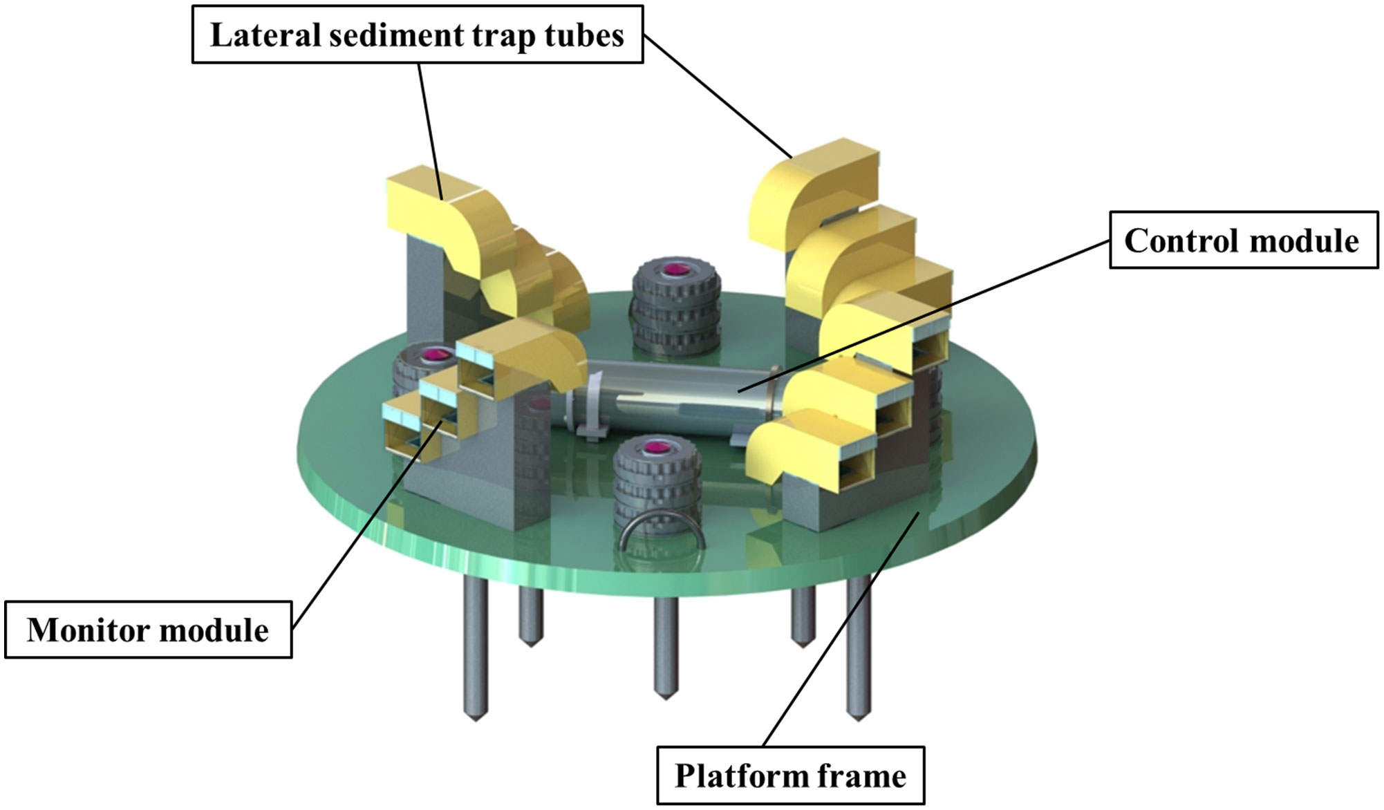
Figure 1 Structure of the 3D monitoring capture device.

The above-mentioned device solves the problem of an insufficient range of observations of highly concentrated fluxes in transport, and can be used to obtain synchronous data on the transported sediment samples. This information can then be used to analyze the factors controlling the transport of the sediment, the typical characteristics of the particles, and changes in the contents of pollutants in different states of the ocean (especially in extreme states, such as storm surges). It provides an accurate means of observing sediment transport, the mechanism of the oceanic carbon cycle, the geo-evolutionary marine mechanism, and the relation between seabed mining and the geological environment in the dynamic domain of the ocean (Bloesch, 1994; Buesseler et al., 2007; Cao et al., 2020; Fan and Xiao, 2021). However, no mature method for the analytical inversion of the data obtained from this device has been developed to date.

To provide an accurate method for the analytical inversion of the above-mentioned trap, the authors of this paper propose a multi-level method to analyze sediment transport based on the inversion of the captured samples, velocity of flow, analysis of the flux in turbidity, and corrected efficiency of capture. We validated and optimized the proposed method based on the results of multi-stage indoor velocity-controlled flume tests. The work here provides a means of reducing the high-resolution 3D time series of the process of transport of sediments.

2 Materials and methods

2.1 Experimental setup

Indoor experiments were carried out by using an annular, multi-stage, velocity-controlled flume to investigate the efficiency of capture of the 3D sediment trap by simulating sediment transport under regular conditions of the marine environment. The entire tank was composed of acrylic material to ensure its transparency, strength and chemical stability. It contained a module to control velocity, a sedimentation module, and an erosion module. The tank is shown in Figure 2. The overall dimensions of the flume, L×W×H, are 180 cm×110 cm×50 cm. There is an internal velocity control module, which can control the flow rate between 0 and 50 cm/s; an internal settling module, with dimensions of 50 cm×40 cm×50 cm; and an erosion soil tank, with dimensions of 50 cm×40 cm×50 cm, as shown in Figure 2A.

FIGURE 2

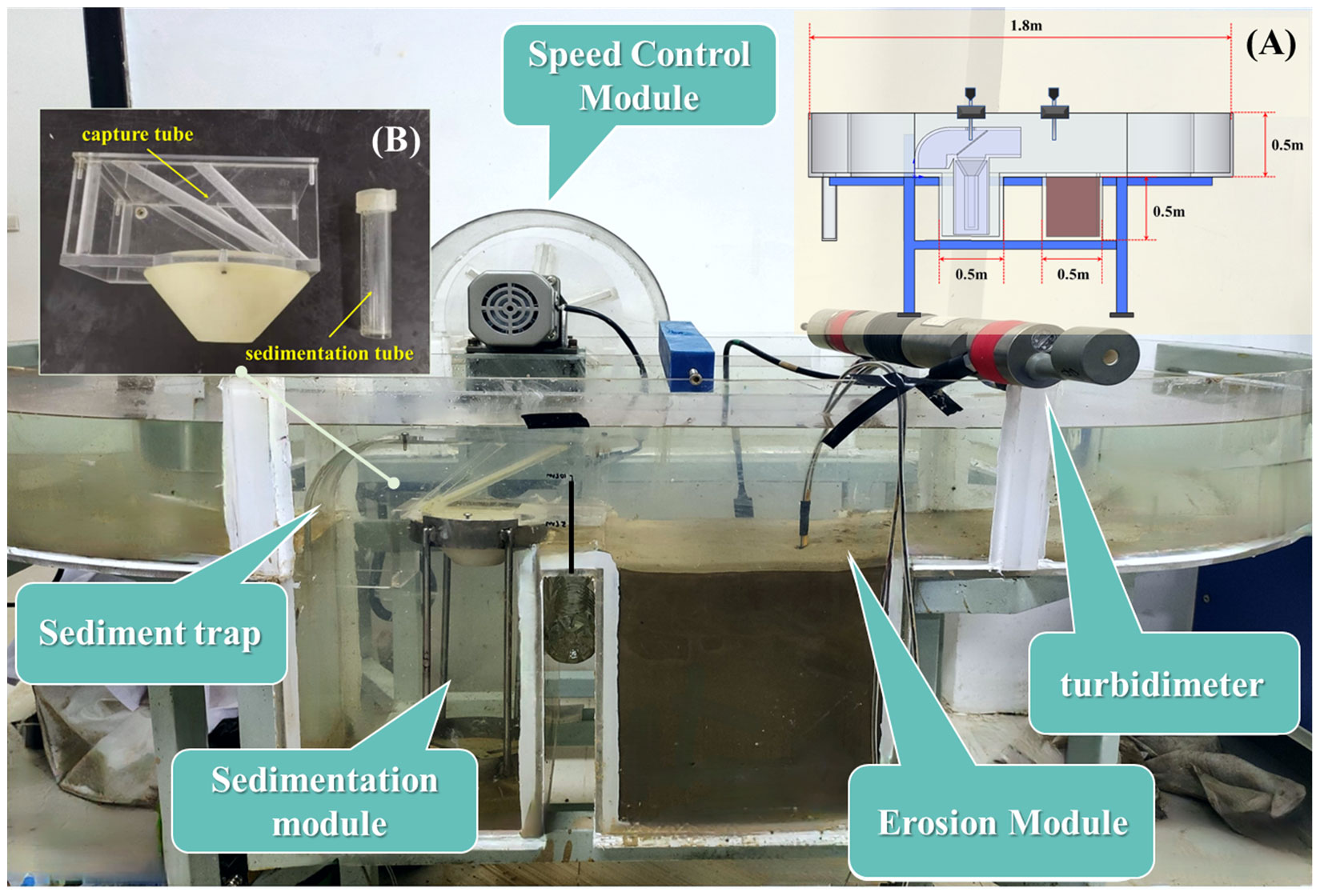
Figure 2 Multistage speed control sink.

The module to control velocity was connected with a motor rod to control the fluid-driving paddles to generate the flow of water by adjusting the frequency of the motor. It could control the rate of horizontal flow of the fluid in the entire flume in the range of 0–50 cm/s, with smooth transitions in velocity to yield scenarios of sediment transport. The outlet of this module was equipped with a closed barrier to ensure that the flow of water was stable in the flume during operation.

Sedimentation set the capture tube placement tank, to reduce the vertical distance between the capture tube and the bottom of the empty tank, so that the sediment settles here. The depth of water could be used to ensure that the capture tube was always in the effective range of capture of the sediment.

The erosion module consisted of an erosion flume that was used to simulate the pattern of initiation of the sediment on the seabed, and enabled the transport of its particles in the entire capture flume. The erosion flume was filled with particles of a test soil of a specific grade, and particles of the sediment were initiated, suspended, pushed, and settled after the liquefaction of the seabed in the simulated environment in the flume. The erosion flume contained a standard scale on the outside, which made it easy to observe the cumulative change in particles of the sediment during the process of initiation of the liquefied soil particles on the seabed. It provided an objective reference to adjust the degree of consolidation and rate of flow of the fluid in soil in a timely manner according to the status of the suspension.

A cohesionless chalky sandy soil conforming to ISO standards was selected for the experiment. We used soil particles with six sets of grain sizes: 0–0.1 mm, 0.1–0.3 mm, 0.3–0.5 mm, 0.5–1 mm, 1–2 mm, and 2–3 mm. All granular soils were configured in equal quantities.

Sediment initiation is complex in nature, and any sediment particle on the seabed surface is random in size, shape and relative position. Some scholars have developed a threshold criterion to determine the threshold condition, among which the most widely used is the Shields curve that can reflect the critical shear and particle characteristics under the critical starting condition of sediment, which was proposed by Shields through a series of tests in the 1930s. The theoretically obtained Shields curve represents the relationship between the Shields parameter and the Reynolds number, and the value of the critical Shields parameter is expressed as a function of the Reynolds number of a particle:

$\begin{array}{ll}R{e}_{*}=\frac{u_{*}d}{v}& \text{(2-1)}\end{array}$

where $R{e}_{*}$ is the Reynolds number of the particle and u_* is the shear velocity.

The Shields curve was fitted to a curve based on measured data and previous supplements (Kramer, 1935). This data set shows considerable dispersion, forming a narrow band rather than a well-defined curve. The inconvenience of the original Shields curve is that the critical shear stress appears on both the transverse and longitudinal axes at the same time as the velocity. Therefore the critical shear stress cannot be determined directly from the raw Shields curve, but needs to be calculated iteratively. Qin proposed a calculation method that can be screened based on the starting equations for individual grain sizes of inhomogeneous silt sand (Qin, 1993), determining the test conditions as shown in Table 1, Eq:

TABLE 1

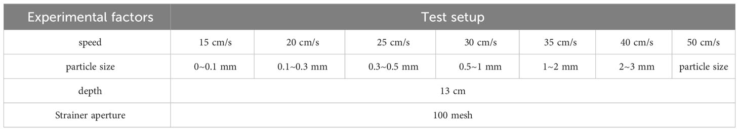
Table 1 Control table for experimental variables.

$\begin{array}{ll}\frac{U_c}{\sqrt{\frac{{\gamma }_s-\gamma }{\gamma }gD}}=0.963\sqrt{0.67+\frac{D_m}{D}}{\left(\frac{h}{D_{90}}\right)}^{1/6}& \text{(2-2)}\end{array}$

Where D_m is the average particle size, D is the particle size, h is the water depth, ${\gamma }_s$ is the particle sediment bulk weight, $\gamma$ is the clear water bulk weight, and U_c is the starting flow rate of the sediment particles.

2.2 Materials

We independently designed and processed the capture tube for the lateral sediment as the main test object, as shown in Figure 2B. The mouth of the capture tube had dimensions of 8 cm × 8 cm. We explored different height-to-diameter ratios of the capture tube, and concluded that the efficiency of capture was the highest it was set to 1:5. We designed an internal sediment strainer to accommodate angles of inclination of 30° and 45°. The flow was less likely to be blocked during the transport of sediment at a high concentration the angle of inclination was 45°, and the intercepted sediment could conveniently fall into the settling tube (Wang et al., 2022). We chose a screen on the premise of reducing the aperture. The difference between the rate of flow inside the capture tube and that outside it gradually increased, and the efficiency of capture decreased once the aperture had increased. We used a 100-mesh screen for interception.

We conducted flume tests by changing the rate of flow, turbidity, concentration, and particle size to explore the Inversion methods based on captured samples, flux analysis method based on the flow rate and turbidity, and determining factors affecting capture efficiency, the analytic inversion method above is shown in Figure 3. When the sediment-carrying fluid passed through the trap tube, the screen in the latter intercepted particles of the sediment with sizes larger than the aperture of the screen. They sank along the capture screen into the settling tube under the action of the inclined screen, and were collected as sediment samples as they settled under the force of gravity of the sediment itself. We used different sequences of samples to develop a method to invert the time series of the sediment based on timed slice unit, formulated a multi-level method to analyze the flux in the lateral transport of the sediment based on the velocity of flow and turbidity, and established a 3D method to analyze the inversion of the sediment by determining the efficiency of capture of the trap.

FIGURE 3

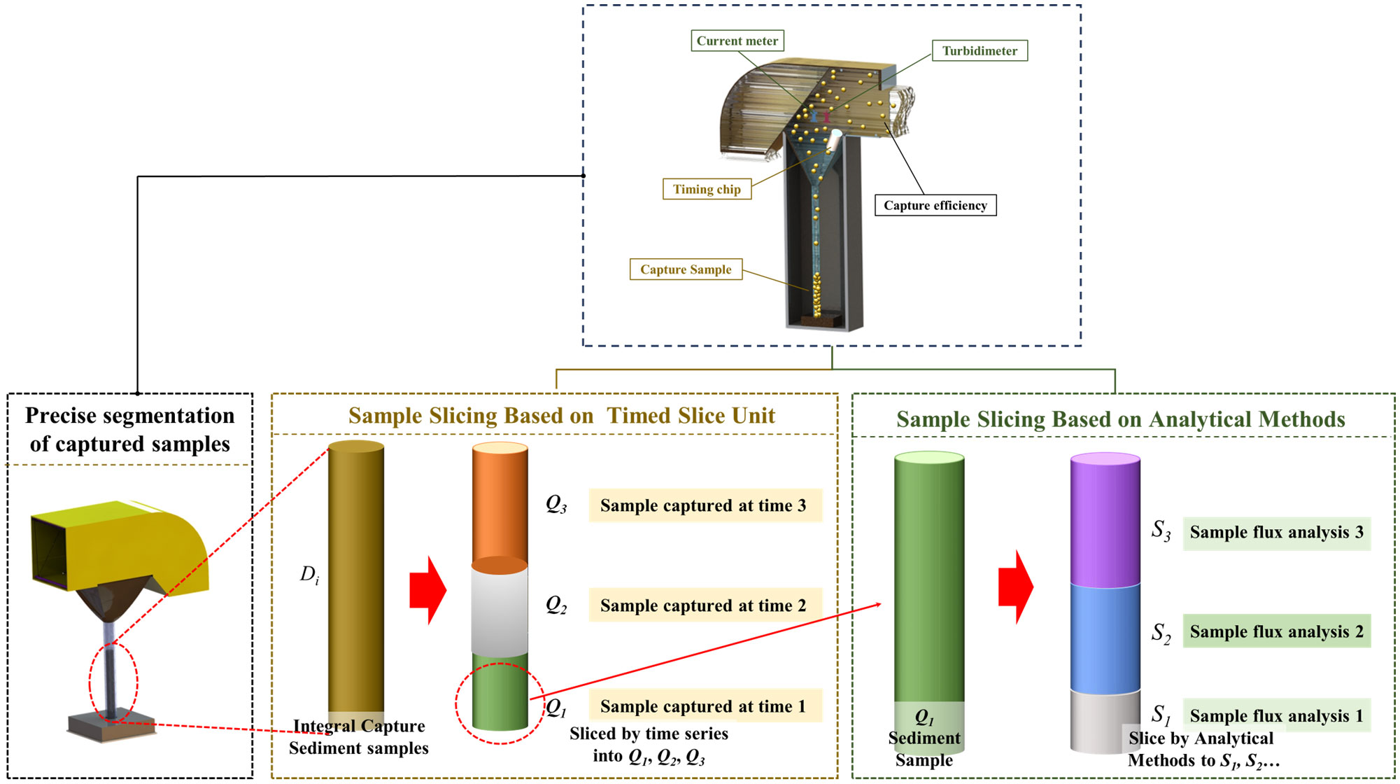
Figure 3 Analysis and inversion methods for sediment traps.

The time series-based method for the inversion of the sediment samples through the timed slice unit was developed by using the captured sediment and examining its properties in each period during its transport. The time was started after each directional slice unit had been ejected, where this occurred at preset intervals inside the capture tube. The slice segmented the sediment samples. Each segment of the column samples was segmented according to time as $Q_1$, $Q_2$, $Q_3$, and so on, and corresponded to the process of transport. This enabled the analytical inversion of the properties of the sediment samples in the time series.

We analytically sliced the collected sediment samples in the time domain to develop a method of analysis based on the rate of flow and turbidity to observe and invert the changes in the flux of the process of transport. A turbidimeter and a flowmeter were installed inside the trap, to continuously monitor the concentration of the sediment SSC_(d,i) and the velocity of flow V_c(d,i). The sediment sample $Q_1$ was further segmented into S₁, S₂, and S₃ according to the nature of the particles or the environment. The velocity of flow inside the device, the concentration of suspended sand in the trap, and the sediment captured by it were analyzed by using an analytical method of sectioning in the time domain. We also used the above data to establish analytical relationships among the velocity of flow along different directions, the turbidity d, and the flux in sediment transport Q_(d,t) over time t. We then used these relationships to analyze each segment of the column and correlate it with the external spatiotemporal conditions. We subsequently analyzed the spatiotemporal sequences of fluxes in the transport of the sediment.

Three-dimensional sediment traps are similar to vertical sediment traps, and their efficiency of capture is likewise influenced by the particle concentration, interval of particle sizes, trap Reynolds number, and rate of fluid flow (Kitheka et al., 2005; McLachlan et al., 2017). We conducted a preliminary investigation into the relationship between the sizes of the captured particulate matter and the overall capture at different rates of flow through flume tests, in order to complement the method of analytical inversion.

The instruments used in the test include a flow meter, a turbidimeter, and a manometer. Among them, LS300-A portable tachometer, the tachometer for the water flushing rotor handheld, range of 0.01 ~ 400 cm/s, real-time display of data, the sensor using fiber-optic light guide, the sampling time of 1 ~ 999 s, independent of the nature of the liquid, the temperature of the influence of the water, suitable for the laboratory tank test.

Canada RBR company’s XR-620CTDTu temperature salt depth multi-parameter water quality monitor, can measure including turbidity and other parameters, and will record the data in real time, the range of 0 ~ 1500 FTU, sampling frequency of 3 s, can be used in narrow waters, accuracy of 0.1 FTU, can be measured continuously for more than 24 h, suitable for laboratory tank experiments.

OCEAN SEVEN 310 CTD multi-parameter water quality meter, can measure the turbidity and other parameters, and will record the data in real time, the range of 0~2500FTU, sampling frequency of 3 s, accuracy of 0.1 FTU, can continue to measure for more than 24 h, suitable for laboratory tank experiments.

Xi’an Wei-Zheng Electronics Technology Company’s CYY2 manometer can realize the measurement of pressure difference in water and record the data in real time. The range of the manometer is 0~5 kPa, and it can measure all kinds of mixed pressures with an accuracy of 0.1% FS, and the sampling frequency can be up to 0.02 s. It can continue to measure for more than 24 h, and it is suitable for the water tank experiments in the laboratory.

The turbidimeter and the manometer used in the tests needed to be calibrated. Conversion relationship between turbidity and suspended sand concentration was obtained by calibration experiments as shown in Figures 4A, B, through the fitting of the two relationship were:

FIGURE 4

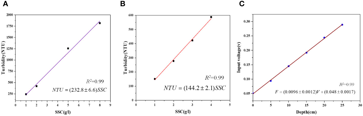
Figure 4 Equipment calibration. (A) Turbidimeter A calibration. (B) Turbidimeter B calibration. (C) Calibration of manometers.

$\begin{array}{ll}NTU=(232.8\pm 6.6)SSC,R^2=0.99& \text{(2-3)}\end{array}$

$\begin{array}{ll}NTU=(144.2\pm 2.1)SSC,R^2=0.99& \text{(2-4)}\end{array}$

The method to calibrate the relationship of conversion between the pressure and voltage was applied by using the pressure at the conventional depth of water, as shown in Figure 4C, and was fitted by:

$\begin{array}{ll}F=(0.0096\pm 0.0012)V+(0.048\pm 0.0017),R^2=0.99& \text{(2-5)}\end{array}$

where F is the force and V represents the voltage.

The pressure due to the depth of water was entered into the formula $P={\displaystyle {\int }_{k_0}^{k_i}\rho g{h}_k}\times S_{(k)}$ to obtain the pressure and voltage, and to thus complete the calibration of the pressure gauge. The pressure due to the depth of the water was used in the formula to derive the correspondence between the pressure and voltage to complete the calibration of the manometer.

2.3 Experimental process

Three types of experiments were conducted in the flume to test the proposed method of sample inversion (A), the method of determining the resolution of flux (B), and the method to determine the efficiency of capture (C). The experimental design is shown in Table 2.

TABLE 2

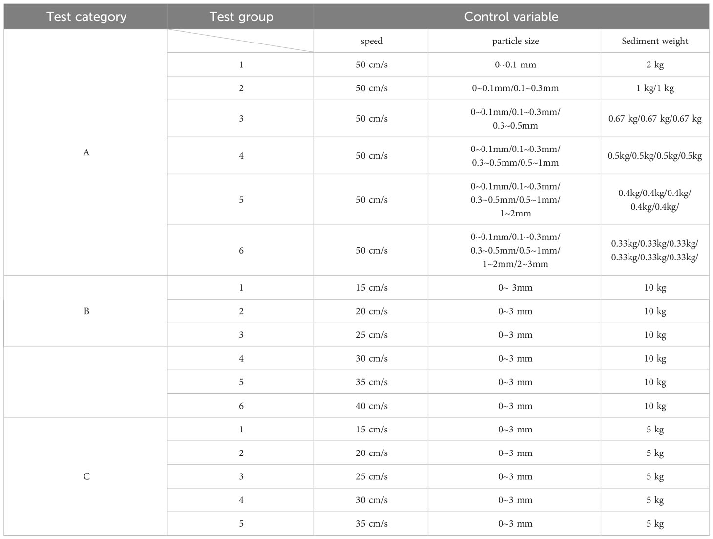
Table 2 Test element setup.

Class A tests were conducted on the captured samples, which were divided into six groups. Each group was assigned a particle size and weight during the test. The same aliquot quantity of particles of different sizes was added to the tank in the experimental groups. The module to control the velocity of flow was then activated to set the rate of flow at the center of the capture tube in the tank to 50 cm/s. The mouth of the capture tube needed to be blocked during its activation to prevent the particles from entering it, and was then opened to capture the particles once they had been flowing for a certain period. We ensured that the settled particles were blocked from the mouth of the trap after 10 min, and cut the fine tube and analyzed the samples to ensure the convergence of their total volume and completeness and once the particles deposited in the trap had completely settled. The tubes were sealed at both ends after each test, and the particulate matter at each level was weighed to determine its mass fraction after all tests had been completed.

Class B tests were used to explored the fluxes in sediment transport, as shown in Figure 5. A flowmeter was installed at the inlet of the capture tube to measure the real-time rate of flow into it. Because some particulate matter particles will simply ignore the filter, the turbidity that actually affects the capture needs to be subtracted from the portion that cannot be captured, so wo turbidimeters were installed at the outlet and the inlet of the capture tube, and the difference between their measurements at the same time was used to calculate the relationship between the actual turbidity under the effect of the interception by the filter screen. A manometer was installed at the bottom of the settling tube inside the capture tube to measure the particulate matter in real time. Owing to the small diameter of the capture tube, the internal capture screen, and the design of the end of the bending structure, the relationship between the velocities of flow inside and outside the capture tube was initially given by using the equation for the correspondence between internal and external flow rates for substitution (Liu et al., 2022). However, we needed to consider the role of the filtering screen as well. Because there was a certain delay in the accumulation of sedimentary particulate matter in the settling tube, it is necessary to be in the static period of time and then read the manometer, to get an accurate sedimentation of particulate matter in the settling tube.

FIGURE 5

Figure 5 Sink Test Scene Layout Diagram.

We installed aperture screens of different sizes, and installed two flowmeters at the same horizontal height inside and outside the capture tube to determine the correspondence between the velocities of internal and external flows. We then added the sediment particles, and activated the module to control the velocity of flow to regulate it at six rates at the mouth of the capture tube. The latter was kept closed from when the module was activated until the rate of flow became constant in each case. When a relatively constant state of turbidity had been reached, the capture tube was opened for 30 min to capture particles of the sediment, and the starting and ending times of the process were recorded. The turbidity was determined based on the difference in measurements between the turbidimeters corresponding to the two time points. The mouth of the capture tube was closed at the end of each period of collection, and readings of the pressure gauge were recorded after a certain period when its value no longer changed. Three sets of parallel control tests were set-up at each value of the rate of flow to obtain three sets of sample values. They were then weighed and correlated with the measured turbidities at the different rates of flow.

Type C tests were conducted to investigate the efficiency of capture. They were divided into five groups, each of which involved adjusting the rate of flow during the test. Particles of all sizes were added to the flume at different initial rates of flow while keeping the capture tube closed during the start-up process. Following stabilization, the capture tube was opened to capture the particles for the same duration for each group. Once the test was stopped, an equal mass of samples was selected from each sampling tube, the particles of each group of sediments were sieved, and the overall particulate matter was weighed against the particulate matter beyond the range of capture to derive the percentage of anomalous particulate matter under each rate of flow. This provided information on the factors influencing the efficiency of capture.

3 Results

3.1 Sediment capture

The collected thin tubes obtained after each cut were arranged at fixed time intervals to obtain six sets of columnar thin tube samples at different time intervals. The particulate fractions used in each period were compared with the samples captured in the corresponding fine tubes during the test. The particles were weighed after having been dried, and were screened to obtain the fraction of particle sizes of each group. The sample resolutions thus obtained are shown in Table 3. The range of particle sizes under each rate of flow as well as the weights of abnormal particles are listed in Table 4.

TABLE 3

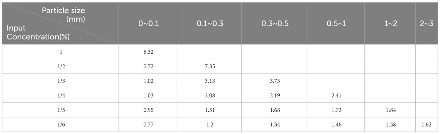
Table 3 Sample timing slicing results.

TABLE 4

Table 4 Capture efficiency probe test results.

3.2 Sediment transport

The correspondences between the internal and external rates of flow when using screen apertures of different sizes as determined by the tests are shown in Figure 6. The correspondences obtained after fitting were:

FIGURE 6

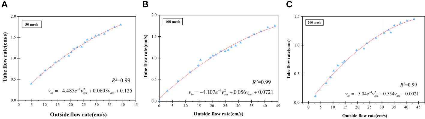
Figure 6 Correspondence between internal and external flow rates. (A) Relationship between internal and external flow rates at 50mesh. (B) Relationship between internal and external flow rates at 100mesh. (C) Relationship between internal and external flow rates at 200mesh.

$\begin{array}{ll}{v}_{in}=-4.485e^{-4}{v}_{out}^2+0.0603v_{out}+0.125,R^2=0.99& \text{(3-1)}\end{array}$

$\begin{array}{ll}{v}_{in}=-4.107e^{-4}{v}_{out}^2+0.056v_{out}+0.0721,R^2=0.99& \text{(3-2)}\end{array}$

$\begin{array}{ll}{v}_{in}=-5.04e^{-4}{v}_{out}^2+0.554v_{out}-0.0021,R^2=0.99& \text{(3-3)}\end{array}$

where $v_{in}$ is the internal flow rate and v_out is the external flow rate.

The turbidities corresponding to the different rates of flow are shown in Figure 7. The average turbidities were 0.15 g/L at a rate of flow of 15 cm/s, 0.28 g/L at 20 cm/s, 0.6 g/L at 25 cm/s, 0.66 g/L at 30 cm/s, 0.7 g/L at 35 cm/s, and 0.82 g/L at a rate of flow of 40 cm/s.

FIGURE 7

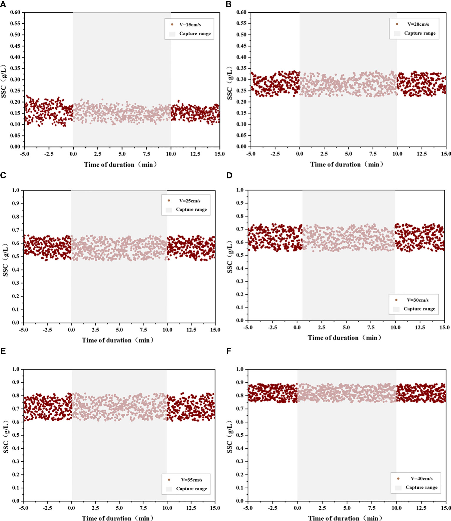
Figure 7 Relationship between turbidity and flow rate. (A) Turbidity change at 15cm/s. (B) Turbidity change at 20cm/s. (C) Turbidity change at 25cm/s. (D) Turbidity change at 30cm/s. (E) Turbidity change at 35cm/s. (F) Turbidity change at 40cm/s.

The results of measurements of the manometers corresponding to the collection of sediments at different rates of flow are shown in Table 5.

TABLE 5

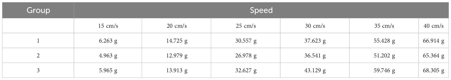
Table 5 Capture collection results.

4 Discussion

4.1 Sample inversion

The data were organized according to the amount of particulate matter captured for each particle size as a percentage of the total amount captured, as shown in Figure 8. It is clear from it that the particle gradation of the captured particulate matter was the same as that of the granular soil configured in the recirculating water tank during the same time period of the test. The grade of the particulate matter obtained from each group of captured particles was approximately equal to that of the input particulate matter, where this verifies that the nature of the particulate matter during sediment transport could be accurately inverted in the time series by using the proposed method of columnar sample slicing inside the capture tube. This provides scientific support for determining the properties of particulate matter during sediment transport. This conclusion is similar to that of the method of sample inversion based on a vertical time series of sediment traps (Chen and Jin, 2013).

FIGURE 8

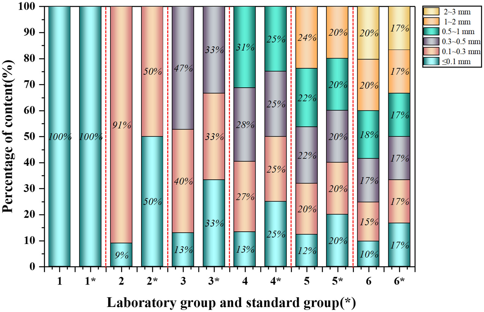
Figure 8 Sample Timing Slicing Analysis.

As the concentration and size of the input particulate matter changed, it was necessary to set-up $m=f(d,c)$ to explore the relationship among particle concentration, particle size, and particle capture under a constant rate of flow. We wrote code in Python to this end, and then used MATLAB to determine the bivariate function based on the relationship between the density and size of the particles as follows:

$\begin{array}{ll}m=29.283+3.505d+1.029c-4.998e^{0.038d+2.853}+4.638e^{-0.001c+2.512},R^2=0.93& \text{(4-1)}\end{array}$

The above formula shows that in the amount of particulate matter captured in the transverse capture tube changed under the influence of the density and size of the particles, such that there was a correspondence among these three variables. This formula is limited to an environment of steady flow, and further research is needed to establish an expression to capture this relationship in more complex environments (Holmedal et al., 2013).

4.2 Transport flux analysis

We introduce a correction factor for the screen of the capture tube to examine the relationship between the internal and external rates of flow, $r_v=\frac{v_{in}}{v_{out}}$. This equation was derived from the results of fitting shown in Figure 6:

$\begin{array}{ll}{r}_v=\{\begin{array}{l}-4.485e^{-4}{v}_{out}+0.0603+\raisebox{1ex}{$0.125$}\!\left/ \!\raisebox{-1ex}{$v_{out}$}\right.,n=50\\ -4.107e^{-4}{v}_{out}+0.056+\raisebox{1ex}{$0.0721$}\!\left/ \!\raisebox{-1ex}{$v_{out}$}\right.,n=100\\ -5.04e^{-4}{v}_{out}+0.554-\raisebox{1ex}{$0.0021$}\!\left/ \!\raisebox{-1ex}{$v_{in}$}\right.,n=200\end{array}& \text{(4-2)}\end{array}$

We used the generalized analytical expression for the turbidity of flow and flux of suspended sand (Haohao et al., 2019) to established an analytical equation based on the effects of variations in the flow field, difference in turbidity, and interception of particles by the screen:

$\begin{array}{ll}{Q}_{(d,t)}=\frac{r_v{\displaystyle {\int }_{i=t-T}^t{V}_{out(d,t)}\times \text{Δ}SS{C}_{(d,t)}}dt}{S\times T}& \text{(4-3)}\end{array}$

where d is the direction of sediment transport, t is the moment, T(s) is the time interval, S(m) is the area of the capture tube opening, SSC is the turbidity, and r_v(m/s) is the filter correction factor.

The data from the turbidimeter and flowmeter were compared with the values derived from the conversion by using the computational manometer, and the resulting relationship between the data is shown in Figure 9. It is evident from it that the theoretical values calculated based on the analytical formulae for the fluxes in the velocity of flow and turbidity satisfactorily corresponded to the actual values converted by the manometer, with a correspondence of $m_a=1.024m_t+0.003m_t^2,R^2=0.99$.

FIGURE 9

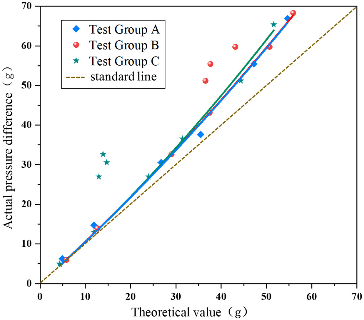
Figure 9 Correspondence between theoretical and actual values.

We used the flume test to analyze the fluxes in sediment transport over a certain period while using the rate of flow, turbidity and time as variables. The total amount of captured sediment with variations in the rate of flow and turbidity verifies the accuracy of the proposed method. This also provides scientific data on the environmental factors influencing sediment transport. This conclusion corresponds to the relationship of flux at a scale of the size of a single grain (Liu et al., 2022).

Following the confirmation of the applicability of the proposed method to analyze changes in turbidity with the rate of flow, further investigation revealed that the theoretical values calculated from the analytical equations did not have a completely linear relationship with the actually values of the captured particles converted by the manometers. Instead, the actual difference in pressure increased with the theoretical difference in it. This can be attributed to the failure to consider the variations in the internal and external turbidities, differences in correspondence between the internal and external rates of flow in case of different particle sizes, and sedimentation during the movement of the fluid carrying the sediments that caused it to move in the vertical direction, such that the fluid perpendicular to the direction of capture generated turbulence inside the capture tube. This caused a small part of the deposited particulate matter to be blocked by the walls of the capture tube. It was then flushed into the capture tube by the horizontally oriented fluid.

4.3 Efficiency of capture

The results of correlations among the rates of flow, intervals of particle size, and occupancy ratios are shown in Figure 10. The left axis represents the interval range of captured grain size, the right axis represents the percentage of abnormal grain size, and the yellow line represents the region of normal grain size.

FIGURE 10

Figure 10 Captured particle size distribution and percentage of anomalies. .

Figure 10 shows that the percentage of abnormally sized particles gradually increased and the efficiency of capture decreased with the increase in the velocity of flow, but this trend gradually decreased in intensity until the percentage of abnormally sized particles began to decrease in the range of velocities of flow of 30–35 cm/s.

The transverse sediment capture efficiency exploration test was carried out through the flume test, and equal mass particles were captured with the flow rate as the variable, and the anomalous change rule of captured particle size with the change of flow rate was found, which explains the effect of flow rate on the capture efficiency. This finding corresponds to that concerning the change in the efficiency of capture under the influence of vertical capture tubes (Butman, 1986).

The variations in particles of anomalous sizes might have been influenced by several factors, which need to be explored in subsequent research in the area. When particles of the sediment were intercepted by the screen in the transverse capture tube during their transport, some of the particles attached to the surface of the screen under the action of inflowing water. This led to small sediment particles being captured by the screen once the diameter of the aperture had been reduced. As the sediment particles began to move, the initial conditions of large particles were more complicated than those of small particles, and this led to the former having a higher viscosity than the latter in the initial process (Taki, 2000). When the sediment-carrying fluid flowed through the 3D trapping device, the flow field changed due to the structure of the device. Smaller particles of the sediment had a tendency to escape along other directions due to disturbances in fluid flow.

4.4 Study limitations

Three-dimensional sediment traps can realize in situ long-term monitoring of sediment transport, and can be applied to inlet, estuary, deep sea and other field monitoring areas. In this paper, we have investigated the effects of particle size and obtained some results, but due to the limitations of the experimental conditions, the study has not taken into account factors such as particle consolidation, hydrodynamic effects, device structure, and filter obstruction. There are still many known influencing factors that need to be investigated. In the future, we will carry out experimental investigations on the influencing factors on the capture efficiency of vertical sediment traps, establish the relationship between various influencing factors and transverse capture tubes, provide scientific guarantee for the design of transverse capture and the correction of capture efficiency, and improve the accuracy and feasibility of the capture of sediment traps through the continuous correction of various influencing factors.

5 Conclusions

Three-dimensional sediment traps can be used to examine the nature of particles of marine sediments as well as changes induced in them by the environment during their transport. They can thus overcome the limitations of traditional means of the indirect estimation of fluxes in the sediment, and the ambiguity of observations of the process of transport. This method thus provides technological support for investigating the geological evolution of the sea, its ecological cycle, fluxes in the marine carbon content, marine engineering, and environmental monitoring during seafloor mining. However, the method to analytically invert the traps during sediment transport is still not sufficiently mature, and thus cannot be applied to in-situ observations. In this paper, we used a 3D sediment trap to proposed methods of sample inversion and the analysis of fluxes in sediment transport, and corrected the efficiency of capture. We validated and optimized the proposed method based on multi-stage, indoor velocity-controlled flume tests. The following conclusions can be drawn from this study:

1. We used the capture and resolution of samples of transported sediments to validate the inversion of the properties of sedimentary particles based on a cut-off value. We also determined the response-related relationship between sediment capture, and the size and density of the sedimentary particles based on the results of the cut-off value.

2. We compared measurements of the velocity of flow, turbidity, and difference in pressure of the transported sediments with theoretical formulae for flux analysis proposed here. The results verified their applicability.

3. We identified the relationships among the rate of flow, particle size, and efficiency of capture based on experiments on the lateral capture tube. This provides a scheme for optimizing the accuracy of the method of trap analysis.

Data availability statement

The original contributions presented in the study are included in the article/supplementary material. Further inquiries can be directed to the corresponding author.

Author contributions

LG: Conceptualization, Data curation, Formal Analysis, Funding acquisition, Investigation, Methodology, Project administration, Software, Supervision, Validation, Visualization, Writing – original draft. ZF: Conceptualization, Data curation, Formal Analysis, Funding acquisition, Investigation, Methodology, Project administration, Software, Supervision, Validation, Visualization, Writing – original draft, Resources, Writing – review & editing. TL: Conceptualization, Software, Writing – review & editing. ZX: Methodology, Project administration, Writing – review & editing. XL: Methodology, Project administration, Writing – original draft. XY: Investigation, Project administration, Writing – review & editing.

Funding

The author(s) declare financial support was received for the research, authorship, and/or publication of this article. This research is financially supported by the Laoshan Laboratory (No. LSKJ202203504); National Natural Science Foundation of China (No. 42176057); National Natural Science Foundation of China (NSFC) (U2006213); National Natural Science Foundation of China (42277138).

Acknowledgments

The authors would like to thank Chen Liu who participated in Generating formulas and Yusen Zhu in output image.

Conflict of interest

The authors declare that the research was conducted in the absence of any commercial or financial relationships that could be construed as a potential conflict of interest.

Publisher’s note

All claims expressed in this article are solely those of the authors and do not necessarily represent those of their affiliated organizations, or those of the publisher, the editors and the reviewers. Any product that may be evaluated in this article, or claim that may be made by its manufacturer, is not guaranteed or endorsed by the publisher.

References

Bloesch J. (1994). A review of methods used to measure sediment resuspension. Hydrobiologia 284 (1), 13–18. doi: 10.1007/bf00005728

CrossRef Full Text | Google Scholar

Buesseler K. O., Antia A. N., Chen M., Fowler S. W., Gardner W. D., Gustafsson O., et al. (2007). An assessment of the use of sediment traps for estimating upper ocean particle fluxes. J. Mar. Res. 65 (3), 345–416. doi: 10.1357/002224007781567621

CrossRef Full Text | Google Scholar

Butman A. C. (1986). Sediment trap biases in turbulent flows: Results from a laboratory flume study. J. Mar. Res. 44, 3, 645–693. doi: 10.1357/002224086788403051

CrossRef Full Text | Google Scholar

Cao Z., Wang D., Zhang Z., Zhou K., Dai M. (2020). Seasonal dynamics and export of biogenic silica in the upper water column of a large marginal sea, the northern south china sea. Prog. Oceanogr 188, 102421.

Google Scholar

Chen L. M., Jin Z. D. (2013). A review of sediment trap techniques and their applications for understanding of settling particle in lakes and oceans. J. Earth Environ.

Google Scholar

Estapa M., Valdes J., Tradd K., Sugar J., Buesseler K. (2020). The neutrally buoyant sediment trap: two decades of progress. J. Atmos. Ocean. Technol. 37 (6).

Google Scholar

Fan J. D., Xiao Z. H. (2021). Analysis of spatial correlation network of china's green innovation. J. Cleaner Prod. 299 (2), 126815. doi: 10.1016/j.jclepro.2021.126815

CrossRef Full Text | Google Scholar

Helley E. J., Smith W. (1971). Development and calibration of a pressure-difference bedload sampler; US department of the interior, geological survey, water resources division. doi: 10.3133/ofr73108

CrossRef Full Text | Google Scholar

Holmedal L. E., Johari J., Myrhaug D. (2013). The seabed boundary layer beneath waves opposing and following a current. Continental Shelf Res. 65, 27–44. doi: 10.1016/j.csr.2013.06.004

CrossRef Full Text | Google Scholar

Horton B. P., Rossi V., Hawkes A. D. (2009). The sedimentary record of the 2005 hurricane season from the Mississippi and Alabama coastlines. Quaternary Int. 195, 15–30. doi: 10.1016/j.quaint.2008.03.004

CrossRef Full Text | Google Scholar

Iseki K. (1981). Vertical transport of particulate organic matter in the deep bering sea and gulf of Alaska[J]. J. Oceanogr. Soc. Japan 37 (3), 101–110. doi: 10.1007/BF02308094

CrossRef Full Text | Google Scholar

Jia Y. G., Tian Z. C., Shi X. F., Liu J. P., Chen J. X., Liu X. L., et al. (2019). Deep-sea sediment resuspension by internal solitary waves in the northern South China sea (vol 9, 12137, 2019). Sci. Rep. 9, 1. doi: 10.1038/s41598-019-53956-y

PubMed Abstract | CrossRef Full Text | Google Scholar

Jiang C. B., Wu Z. Y., Jie C., Liu J. (2014). Review of sediment transport and beach profile changes under storm surge. J. Changsha Univ. Sci. Technol. (Nat. Sci.) 11 (1). doi: 1672-9331(2014)01-0001-09

Google Scholar

Kitheka J. U., Obiero M., Nthenge P. (2005). River discharge, sediment transport and exchange in the tana estuary, kenya. Estuar. Coast. Shelf Sci. 63 (3), 455–468. doi: 10.1016/j.ecss.2004.11.011

CrossRef Full Text | Google Scholar

Kramer H. (1935). Sand mixtures and sand movements in fluvial models. Transaction ASCE 100, 798–878. doi: 10.1061/TACEAT.0004653

CrossRef Full Text | Google Scholar

Kraus N. C. (1987). Application of portable traps for obtaining point measurements of sediment transport rates in the surf zone. J. Coast. Res. 3 (2), 139–152. doi: 10.2307/4297270

CrossRef Full Text | Google Scholar

Liu J. P., Milliman J. D., Gao S., Cheng P. (2004). Holocene development of the yellow river's subaqueous delta, North Yellow Sea. Mar. Geol. 209, 45–67. doi: 10.1016/j.margeo.2004.06.009

CrossRef Full Text | Google Scholar

Liu T., Fei Z. H., Guo L., Zhang J. R., Zhang S. T., Zhang Y. (2022). Newly designed and experimental test of the sediment trap for horizontal transport flux. Sensors 22 (11), 16. doi: 10.3390/s22114137

CrossRef Full Text | Google Scholar

Liu X. L., Lu Y., Yu H. Y., Ma L. K., Li X. Y., Li W. J., et al. (2022). In-situ observation of storm-induced wave-supported fluid mud occurrence in the subaqueous Yellow River delta. J. Geophysical Research: Oceans 127 (7), e2021JC018190. doi: 10.1029/2021JC018190

CrossRef Full Text | Google Scholar

Liu X. L., Wang Y. Y., Zhang H., Guo X. S. (2023). Susceptibility of typical marine geological disasters: an overview. Geoenvironmental disaster 10, 10. doi: 10.1186/s40677-023-00237-6

CrossRef Full Text | Google Scholar

Liu X. L., Zhang H., Zheng J. W., Guo L., Jia Y. G., Bian C. W., et al. (2020). Critical role of wave-seabed interactions in the extensive erosion of Yellow River estuarine sediments. Mar. Geology 426, 106208. doi: 10.1016/j.margeo.2020.106208

CrossRef Full Text | Google Scholar

Lowe D. R. (1982). Sediment gravity flows; II, depositional models with special reference to the deposits of high-density turbidity currents. J. Sediment. Res. 52 (1), 279–297. doi: 10.1306/212F7F31-2B24-11D7-8648000102C1865D

CrossRef Full Text | Google Scholar

McLachlan R. L., Ogston A. S., Allison M. A. (2017). Implications of tidally-varying bed stress and intermittent estuarine stratification on fine-sediment dynamics through the Mekong’s tidal river to estuarine reach. Cont. Shelf Res. 147, 27–37.

Google Scholar

Mikkelsen O. A. (2002). Examples of spatial and temporal variations of some fine-grained suspended particle characteristics in two Danish coastal water bodies. Oceanologica Acta 25 (1), 39–49. doi: 10.1016/S0399-1784(01)01175-6

CrossRef Full Text | Google Scholar

Navratil O., Esteves M., Legout C., Gratiot N., Nemery J., Willmore S., et al. (2011). Global uncertainty analysis of suspended sediment monitoring using turbidimeter in a small mountainous river catchment. J. Hydrol. 398 (3-4), 246–259.

Google Scholar

Nelson J. M., Shreve R. L., McLean S. R., Drake T. G. (1995). Role of near-bed turbulence structure in bed-load transport and bed form mechanics. Water Resour. Res. 31 (8), 2071–2086. doi: 10.1029/95wr00976

CrossRef Full Text | Google Scholar

Nittrouer C. A. (1999). STRATAFORM: overview of its design and synthesis of its results. Mar. Geology 154 (1-4), 3–12. doi: 10.1016/s0025-3227(98)00128-5

CrossRef Full Text | Google Scholar

Niu J. W., Xu J. S., Li G. X., Dong P., Shi J. H., Qiao L. L. (2020). Swell-dominated sediment re-suspension in a silty coastal seabed. Estuar. Coast. Shelf Sci. 242, 9. doi: 10.1016/j.ecss.2020.106845

CrossRef Full Text | Google Scholar

Ogston A. S., Cacchione D. A., Sternberg R. W., Kineke G. C. (2000). Observations of storm and river flood-driven sediment transport on the northern California continental shelf. Continental Shelf Res. 20 (16), 2141–2162. doi: 10.1016/s0278-4343(00)00065-0

CrossRef Full Text | Google Scholar

Peng Y., Steel R. J., Rossi V. M., Olariu C. (2018). Mixed-energy process interactions read from a compound-clinoform delta (paleo–orinoco delta, trinidad): preservation of river and tide signals by mud-induced wave damping. J. Sedimentary Res. 88 (1), 75–90. doi: 10.2110/jsr.2018.3

CrossRef Full Text | Google Scholar

Qin R. Y. (1993). Bed load transport of non-uniform sand mixture. J. Sediment Res. doi: 10.1080/02626667.2019.1615621

CrossRef Full Text | Google Scholar

Reeder D. B., Ma B. B., Yang Y. J. (2011). Very large subaqueous sand dunes on the upper continental slope in the South China Sea generated by episodic, shoaling deep-water internal solitary waves. Mar. Geology 279 (1-4), 12–18. doi: 10.1016/j.margeo.2010.10.009

CrossRef Full Text | Google Scholar

Taki K. (2000). Critical shear stress for cohesive sediment transport 3, 6, 53–61. doi: 10.1016/S1568-2692(00)80112-6

CrossRef Full Text | Google Scholar

Tananaev N. I., Makarieva O. M., Lebedeva L. S. (2016). Trends in annual and extreme flows in the Lena River basin, Northern Eurasia[J]. Geophys. Res. Lett. 43 (20). doi: 10.1002/2016GL070796

CrossRef Full Text | Google Scholar

Wang C., Guo L., Zhang S. T., Fei Z. H., Xue G., Yang X. Q., et al. (2022). The numerical investigation of the performance of a newly designed sediment trap for horizontal transport flux. Sensors 22 (19), 16. doi: 10.3390/s22197262

CrossRef Full Text | Google Scholar

Wen M., Shan H., Zhang S., Guo L., Liu X., Jia Y. (2016). Resuspension of sediments along the bottom boundary layer:a review. Mar. Geology Quaternary Geology 36 (1), 177–188. doi: 10.16562/j.cnki.0256-1492.2016.01.018

CrossRef Full Text | Google Scholar

Yang Z. S., Ji Y. J., Bi N. S., Lei K., Wang H. J. (2011). Sediment transport off the Huanghe (Yellow River) delta and in the adjacent Bohai Sea in winter and seasonal comparison. Estuar. Coast. Shelf Sci. 93 (3), 173–181. doi: 10.1016/j.ecss.2010.06.005

CrossRef Full Text | Google Scholar

Yu H. Y., Liu X. L., Lu Y., Li W. J., Gao H., Wu R. Y., et al. (2022). Characteristics of the sediment gravity flow triggered by wave-induced liquefaction on a sloping silty seabed: An experimental investigation. Front. Earth Sci. 10. doi: 10.3389/feart.2022.909605

PubMed Abstract | CrossRef Full Text | Google Scholar

Zhan W., Wu J., Wei X., Tang S., Zhan H. (2019). Spatio-temporal variation of the suspended sediment concentration in the Pearl River Estuary observed by MODIS during 2003–2015. Cont. Shelf Res. 172, 22–32. doi: 10.1016/j.csr.2018.11.007

CrossRef Full Text | Google Scholar