RFI mitigation for 2D Synthetic Aperture Interferometric Radiometers using combined theoretical and machine learning technique

Synthetic Aperture Interferometric Radiometer (SAIR) as one of the most advanced instruments for Sea Surface Salinity (SSS) observation, has been in service on SMOS mission for years and is planned on the Chinese Ocean Salinity Satellite in the near future. However, a lot of Radio Frequency Interference (RFI) emissions are found in SMOS views, which contaminate the brightness temperature measurements of the SAIR instrument, and further impede the retrieval of SSS fields. Concerning SAIR’s operating mode, this study proposes an RFI mitigation method comprising two algorithms for co- and cross-polarization, respectively. First, RFI signatures are identified based on a series of thresholds defined by radiation theory, and then mitigated through a simple machine learning technique of Support Vector Regression (SVR), leveraging either SAIR’s multi-angle measurements or sea surface roughness descriptors, depending on the specific polarization mode. Finally, the outputs of all polarizations are merged and written back to the Level 1C brightness temperature product as the final result. Using the proposed method, the notable outliers arose from RFI contamination are attenuated, and the variation of standard deviations over nearby snapshots is smoothed, as expected on a homogeneous ocean. Furthermore, with the official L2OS software implementing the SSS retrieval procedure from the rewritten Level 1C brightness temperatures, the data re-gain of SSS fields is achieved in some places that are not attainable for the current SMOS Level 2 SSS products, with a reasonable error compared to WOA2009 SSS, confirming the validity of the proposed method. Hopefully, this work could provide a practical solution to current and future SAIR observing predicaments.

1 Introduction

Ocean salinity is one of the most critical hydrological parameters. Studying its distribution and variation is important for understanding water mass circulation and air-sea interactions (Li et al., 2016). Around the world, there have been three Earth observation satellites for ocean salinity, named SMOS, Aquarius/SAC-D and SMAP. However, Aquarius/SAC-D ended its operation in 2015 (Lagerloef et al., 2008; Brown et al., 2015), and SMAP specializes in the measurement of soil moisture rather than ocean salinity (Entekhabi et al., 2009). That leaves SMOS the most potent satellite for current SSS (Sea Surface Salinity) remote sensing, and its only valid sensor MIRAS (Microwave Imaging Radiometer using Aperture Synthesis), as an instance of SAIR (Synthetic Aperture Interferometric Radiometer), the paradigm of the future SSS observation instrument.

The novelty of SAIR lies in the application of the Synthetic Aperture technique, which was initially used in SAR (Synthetic Aperture Radar) to achieve high spatial resolution and is now playing a broader role in other domains, such as the underwater SAS (Synthetic Aperture Sonar) (Yang, 2023; Zhang et al., 2023) and the discussed SAIR. The envision of SAIR was proposed early in 1983 (Levine and Good, 1983), but not until 2009 the realization of MIRAS did the technique find its way into supporting SSS observation (Font et al., 2001), mainly because the optimal bandwidth for the task is L-band, a relatively low frequency that would otherwise adopt an oversized real aperture. Inspired by the performance of MIRAS, China is now anticipating a new Chinese Ocean Salinity Satellite in 2024 carrying a similar SAIR payload called IMR (Interferometric Microwave Radiometer) (Li et al., 2022).

The preferable L-band (between 1400 and 1427 MHz) allocated for SSS remote sensing is reserved and should have been protected from artificial emissions according to provision No.5.340 of RR (Radio Regulations) of ITU-R (the International Telecommunication Union Radiocommunications Sector) (Oliva et al., 2016). Unfortunately, SMOS images have shown a large amount of RFI (Radio Frequency Interference) emissions around the world. Although most of them are on lands, the side lobes or “tails” of the impulse response could extend over significant parts of oceans, making the observed sea surface brightness temperatures untruthful, and the retrieved SSS inaccurate or even corrupted (Camps et al., 2010; Skou et al., 2010; Johnson and Aksoy, 2011), especially in coastal waters where the socio-economic interests are significant.

This manuscript first briefly reviews the existing studies on RFI detection for SMOS mission. Nevertheless, the previous researches either simply flagged the contamination and brutally discarded the associated measurements, leading to massive data loss and the collapse of SSS inversion. Or the specific implementation involving the entire signal flow chain was so complicated that only suitable for case study instead of batch processing. Therefore, despite all the efforts, the overall condition remains severe, and doable techniques for the observed data recovery from RFI contaminated scenarios are still inadequate.

In this paper, a pragmatic RFI detection and mitigation method is proposed based on the radiation theory, combined with the unique operating pattern of 2D SAIR instruments, as well as machine learning techniques. The approach is easily implemented and reliable in canceling or at least attenuating RFI impacts on brightness temperature measurements, thus facilitating the re-acquisition of ocean salinity fields in contaminated areas where the current satellite salinity products are not available. The method is validated on brightness temperatures in the angular and space domains, in addition to the variation of standard deviations over neighboring oceans. Furthermore, it is corroborated by the actual data gain on the SSS fields retrieved from the altered brightness temperatures leveraging SMOS official L2OS Operational Processor Software, with an acceptable data accuracy compared to the World Ocean Atlas 2009 (WOA2009) SSS. We hope this study could serve as a ready-to-use solution for the current SMOS mission and a reference for the Chinese Ocean Salinity Satellite in the near future.

2 Related works

Many researchers have been studying RFI detection and attenuation of its impact on Earth observations since the SMOS mission was launched. In general, two categories of methods established on two stages of the signal flow have been developed, one is on the so-called “visibilities” of SMOS Level 1A products, and the other is on the brightness temperatures organized in Level 1B or Level 1C products.

In the first case, (Anterrie, 2011) was among the earliest to evidence RFI on the complex visibilities and to give an initial quantification. He later modeled RFI regarding brightness temperatures and ground locations to achieve mitigation by minimizing a local criterion (Anterrieu et al., 2016). (Castro et al., 2013) introduced the sun effect cancellation technique to RFI mitigation of small-to-moderate emissions when no strong unresolved sources existed. (Camps et al., 2014) applied the beam- and null-steering techniques to interpret the synthetic aperture array as a real aperture and simulated RFI by padding zeroes in the source position, but the method may be troublesome to implement due to its strict dependency on the accuracy of RFI localization. Some works have been dedicated to the geolocation matter. For example, (Soldo et al., 2014) tried to create a synthetic signal simulating the visibility of an RFI emission and then subtract it from the measured visibility, but the exact signal recreation is hardly achievable. (Park et al., 2016) has discussed MUltiple SIgnal Classification direction-of-arrival estimations for RFI detection. (Jin et al., 2022b) provided a finer accuracy by noticing the difference on multiple snapshots on the premise that the location of RFI sources remains unchanged, and further addressed the low to moderate contamination cases based on the point-ripple characteristic of RFI sources (Jin et al., 2022a). The above methods of tacking RFI in the very early stage of the signal processing chain, while theoretically feasible, are very likely to propagate errors through the data flow, leading to exacerbated inaccuracies on the retrieved SSS.

The actual implementation for the second category of approaches is more practical and viable when the target is the brightness temperature maps in SMOS Level 1B or Level 1C products. (Camps et al., 2011) has illustrated two RFI detection and mitigation algorithms for dual- and full-polarization modes respectively, using some thresholds to differentiate contaminated measurements, which set the tone for follow-up studies. The SMOS team has been presenting general overviews of the RFI situation and developing algorithms established on nominal thresholds, so as to detect coordinates of RFI sources that can then be provided to national authorities (Oliva et al., 2012; Daganzo-Eusebio et al., 2013; Oliva et al., 2013; Oliva et al., 2016), as their interest is to switch off the illegal emitters directly and thoroughly. (Soldo et al., 2015) applied two adaptive thresholds determining high brightness temperatures and high gradients to localize RFI sources on the snapshot level. (Kristensen et al., 2012) described the potential of the third and fourth Stokes parameters to detect RFI, and (Misra and Ruf, 2012) proposed detecting in the angular domain. In addition, (Xu et al., 2022) proposed an RFI quantitative measurement indicating the probability or intensity of the contamination. However, these methods provided no instructions on how to attenuate RFI impacts. In general, methods based on brightness temperature maps are more effective in pinpointing RFI sources and thus as proof for international cooperation, but not adequate to mitigate the contamination on satellite measurements in the presence of existing RFI sources without massive data loss.

3 Preliminaries

3.1 Theoretical description

The sensor MIRAS (Microwave Imaging Radiometer using Aperture Synthesis) onboard SMOS (Soil Moisture and Ocean Salinity) and the resemblant IMR (Interferometric Microwave Radiometer) on the projected Chinese Ocean Salinity Satellite both adopt a Y-shaped antenna array consisting of three deployable arms. For MIRAS, 69 antennas are equally distributed over the three arms (McMullan et al., 2008), and IMR has 56 antennas settled (Li et al., 2022). The interferometric measurement of SAIR instruments, termed visibility, is the complex cross-correlation between signals collected by two antennas with overlapping fields of view. Since the time delay from a given geographical point to the two antennas provides an exponential term relative to the antenna spacing, the visibility of the pair of antennas is equivalent to the Fourier transform of the brightness temperature (Corbella et al., 2009). Accordingly, the brightness temperature can be reconstructed from the visibility by some inverse procedure.

By definition, the brightness temperature Tb is the function of SST (Sea Surface Temperature) and the surface emissivity e in the specified spectral band, i.e., L-band in the case of SSS measuring (Equation 1),

$\begin{array}{ll}Tb=e\times SST& \text{(Eq. 1)}\end{array}$

Assuming thermodynamical equilibrium and applying the Kirchhoff laws, the emissivity e is equal to the residual after subtracting the reflectivity R (Equation 2),

$\begin{array}{ll}e=1-R& \text{(Eq. 2)}\end{array}$

Based on the Fresnel reflection laws, reflectivity R is defined with the seawater dielectric constant ϵ and the incidence angle θ (Equations 3 and 4),

$\begin{array}{ll}{R}^h={\left|\frac{\cos \theta -\sqrt{ϵ-{\sin }^2\theta }}{\cos \theta +\sqrt{ϵ-{\sin }^2\theta }}\right|}^2& \text{(Eq. 3)}\end{array}$

$\begin{array}{ll}{R}^v={\left|\frac{ϵ\cos \theta -\sqrt{ϵ-{\sin }^2\theta }}{ϵ\cos \theta +\sqrt{ϵ-{\sin }^2\theta }}\right|}^2& \text{(Eq. 4)}\end{array}$

Therefore Tb^h and Tb^v for a flat sea surface can be expressed as(SMOS, 2023c) (Equations 5 and 6),

$\begin{array}{ll}T{b}_{(\theta ,SST,SSS)}^h=(1-R_{(\theta ,ϵ)}^h)·SST& \text{(Eq. 5)}\end{array}$

$\begin{array}{ll}T{b}_{(\theta ,SST,SSS)}^v=(1-R_{(\theta ,ϵ)}^v)·SST& \text{(Eq. 6)}\end{array}$

For a smooth sea surface, the seawater dielectric constant ϵ depends on the temperature and salinity of the water. In fact, the computation of ϵ is straightforward and sufficiently accurate, using for example the Klein and Swift model (Klein and Swift, 1977) proposed early in 1977. In the real world, however, the sea surface can never be perfectly flat, with roughness at different scales created by wind waves and swells, as well as their interactions, resulting in slight modification on the reflectivity R from Fresnel equations. In such circumstances, the brightness temperature should be the sum of two terms, one from the completely flat sea as described above, and the other is the incremental brightness temperature due to the surface roughness $\overline{P_{rough}}$ (Equation 7).

$\begin{array}{ll}Tb=T{b}_{flat}(SSS,SST,\theta )+T{b}_{rough}(SSS,SST,\theta ,\overline{P_{rough}})& \text{(Eq. 7)}\end{array}$

3.2 Operating pattern

For better performance of the SAIR instrument on SSS observation, perhaps the most profound design for MIRAS, and so inherited by IMR, is the multi-angle measuring approach. This means each geographical point will be observed from over a wide range of incidence angles, thus providing a series of brightness temperature measurements relative to various incidence angles for a single point.

As for the operating mode, IMR is planned to operate in full polarization (Li et al., 2022), and MIRAS has already been in full polarization after September 2010. That said, four polarization modes, HH, VV, VH, HV, are interlacedly and alternatively activated, with the integration time τ = 1.2s (Figure 1) (Martin-Neira et al., 2002). In this frame, the four Stokes parameters T_xx, T_yy, Re{T_xy} and Im{T_xy} are obtained during four switching intervals, and can be modified as below (SMOS, 2023c) (Equation 8).

Figure 1

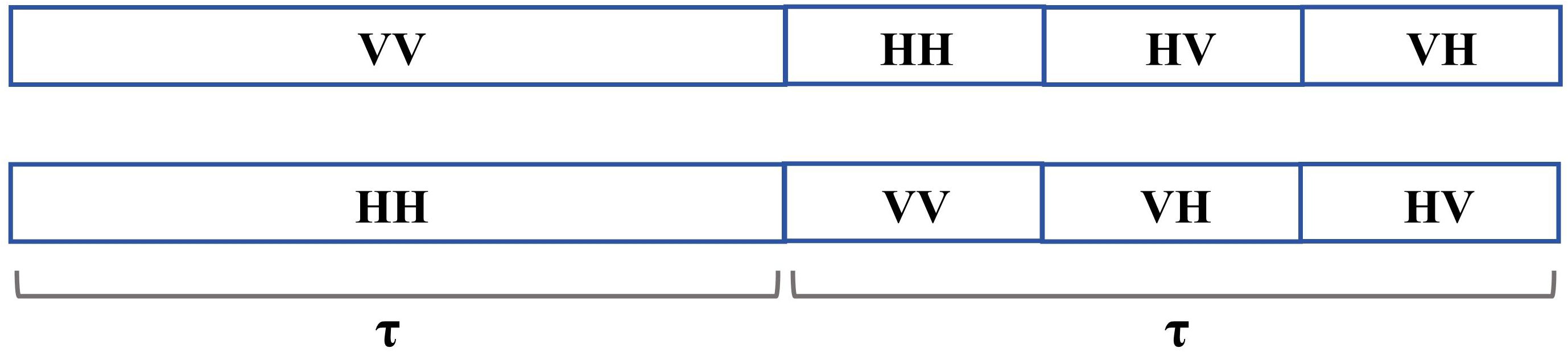
Figure 1 Full polarization. MIRAS polarimetric mode-switching sequences with interlacing and alternating polarization.

$\begin{array}{ll}\left\{\begin{array}{c}A1\\ A2\\ A3\\ A4\end{array}\right\}=\frac{{\lambda }^2}{KB\eta }\left|\begin{array}{c}{\langle \left|E_h\right|\rangle }^2\\ {\langle \left|E_u\right|\rangle }^2\\ 2\mathrm{Re}\langle \left|E_u{E}_h^{\ast }\right|\rangle \\ 2\mathrm{Im}\langle \left|E_u{E}_h^{\ast }\right|\rangle \end{array}\right|=\left\{\begin{array}{c}Txx\\ Tyy\\ 2\mathrm{Re}(Txy)\\ 2\mathrm{Im}(Txy)\end{array}\right\}& \text{(Eq. 8)}\end{array}$

Where λ is the radiometer’s wavelength, K is the Boltzmann constant, B is the bandwidth, and η is the medium impedance (air). E_h and E_v are the two orthogonal components of the plane wave.

4 Materials

While a majority of RFI sources are located on continents, they may inevitably be distributed over oceans, such as from wireless devices if not properly filtered (Oliva et al., 2012). In addition, an even greater threat comes from very strong RFI emissions on coastal lands, which could cause broad and extensive contamination on nearshore waters (Oliva et al., 2016). As a consequence, these waters often suffer from severe interference, hampering measurements of sea surface brightness temperatures and thus the retrieval of SSS fields.

As China’s territorial and adjacent waters, the Bohai Sea, Yellow Sea, East China Sea and South China Sea are hard hit by RFI contamination associated with massive socioeconomic activities and heavy marine transportation tasks. Under such circumstances, ocean salinity observation by remote sensing satellites is so greatly impeded that large areas are discarded in the current SMOS Level 2 SSS products, and even bigger losses after data quality control in Level 3 and Level 4 products. Therefore, this study takes these areas within the range of 4^°N −42^°N, 105^°E −130^°E as the object to inspect the proposed RFI detection and mitigation method, but should note that the approach is not restricted to any specific region. Figure 2 displays SMOS daily global Level 3 Sea Surface Salinity maps from two reprocessed organizations, BEC (Barcelona Expert Center) (BEC, 2023) and CATDS (Centre Aval de Traitement des Donn Données SMOS) (CATDS, 2023), both with blanks in the region of interest (red boxes), indicating the corruption of SSS retrieval due to strong RFI presence.

Figure 2

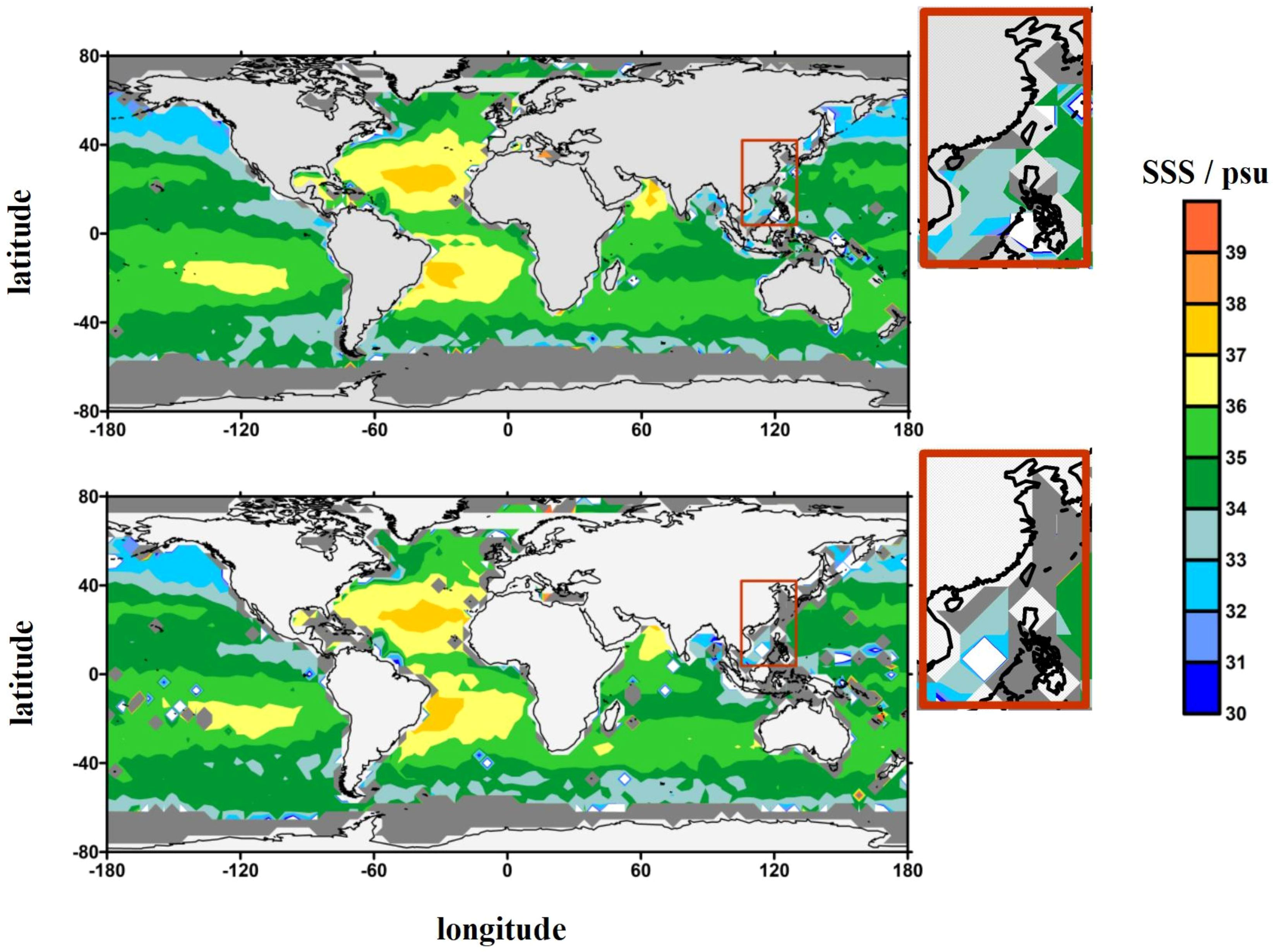
Figure 2 Global Level 3 SSS products. The region of interest (4^°N − 42^°N,105^°E − 130^°E) is marked with a red box on global maps and zoomed in next to them. Light gray represents lands and dark gray represents blanked areas where the measured brightness temperatures are unqualified for ocean salinity retrieval. Level 3 SSS products are provided by two reprocessed teams. The upper one is from BEC-Barcelona Expert Center, Spain, and the bottom one is from CATDS - Centre Aval de Traitement des Données SMOS, France.

As the only 2D SAIR in-service at the moment, SMOS MIRAS provides Level 1C products containing multi-angle brightness temperature measurements, Level 2 Ocean Salinity (OS) products comprising SSS fields, and Auxiliary ECMWF products storing the geophysical parameters from European Centre for Medium-Range Weather Forecasts (ECMWF), all openly available through ESA SMOS Online Dissemination Service (SMOS, 2023a), each per SMOS half-orbit (satellite pass). In addition, the restricted AUX SSS products referring to Sea Surface Salinity monthly mean values imported from World Ocean Atlas 2009 (WOA2009) are also accessible upon request to the SMOS team. Table 1 lists the descriptions of the products used in this study.

Table 1

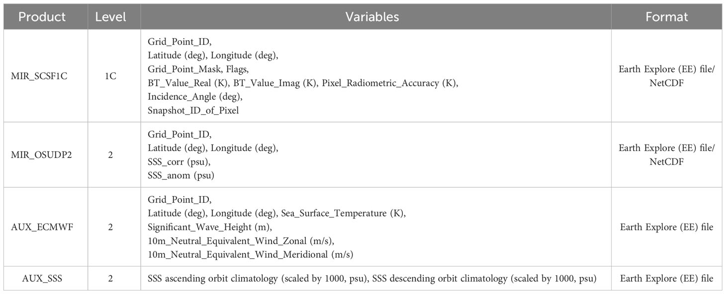
Table 1 The SMOS products used in the study.

5 Methodology

In light of the actual performance of MIRAS and the pre-simulation of IMR, both SAIR instruments should operate in full polarization mode, including the co-polarization HH and VV, and the cross-polarization HV and VH. From the hardware point of view, the co-polarization sets all three arms of the instrument to the same polarization, H or V. While with the cross-polarization, one of the three arms will be polarized in a different direction from the others. For HV-polarization, one arm is in H and the others in V, and the opposite for VH-polarization. The divergent hardware behaviors lead to differences in the satellite’s Level 1C brightness temperature fields. The co-polarization HH and VV generate real values whose imaginary part is zero, while the cross-polarization HV and VH produce complex brightness temperatures comprising both real and imaginary parts. Therefore, two algorithms are developed separately to accommodate the characteristics of co- and cross-polarization, respectively, with each subdivided into RFI detection and RFI mitigation phases. Figure 3 demonstrates the overall processing flow of the proposed method, and the following will explain every step in detail.

Figure 3

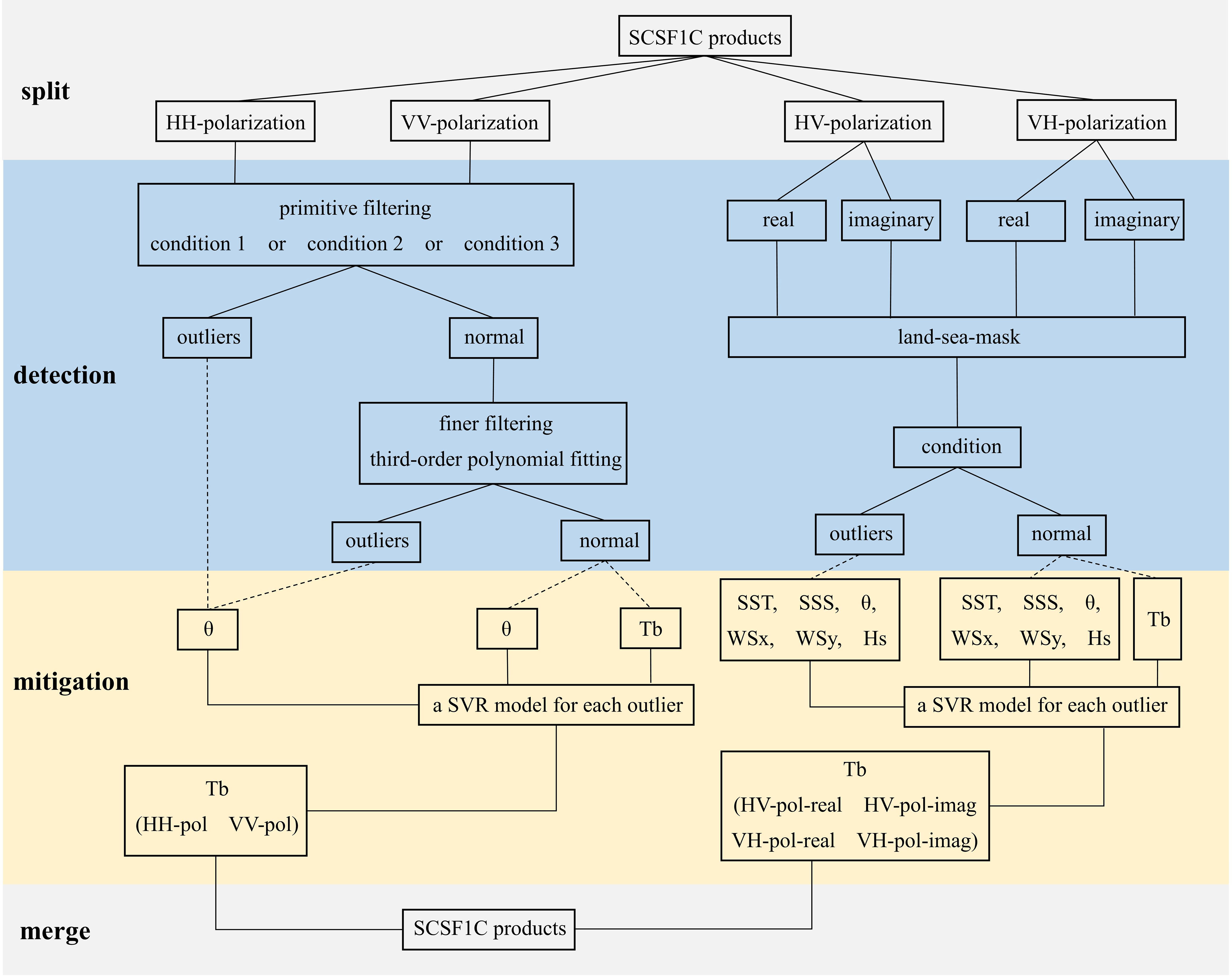
Figure 3 Processing flow of the proposed method. The solid line is the real processing flow. The dashed line represents the parameters in the lower end are related to each item of the upper end, and these parameters are extracted from AUX ECMWF or AUX_SSS products.

5.1 Co-polarization

5.1.1 RFI detection

The RFI detection for co-polarization consists of two hierarchical filtering stages, including a primitive one applied on the half-orbit level (a satellite pass) and the finer one conducted on every grid point successively. In the stage of primitive filtering, the measurement will be flagged as an outlier when the observed brightness temperature meets one of the following conditions:

1. Tb_observe > 330K

2. Tb_{observe <} 50K

3. |Tb_observe − Tb_model| > 60K where Tb_model = Tb_flat + Tb_rough, of which the first term Tb_flat can be directly calculated by Equations 3–6, with the seawater dielectric constant ϵ deduced from the Klein and Swift model (see Supplementary Material for coefficients). The second term Tb_rough is hardly obtained with sufficient precision by any physical model, but it can be concluded that in most cases it should not exceed 10K (SMOS, 2023c).

The underlying logic of these conditions is that the observed Tb_observe should not be beyond or below the maximum or minimum brightness temperature of any blackbody, nor should it exceed the theoretical Tb_model for that particular grid over a certain value. For the first condition, some studies (Oliva et al., 2013; Soldo et al., 2015) may have chosen 350K as the upper limit that could possibly be emitted from the earth, but we consider dropping to 330K (≈ 57^°C) to be more rigorous yet spare enough since our focus is only on oceans. The second condition chooses 50K as a rather relaxed threshold, for nothing on the earth can be this cold, and the measurements must be problematic for some reason. As for the third condition, (ARGANS, 2023b) takes a threshold of 50K to determine any anomalies. We raise it to 60K to accommodate contributions from roughness which are not involved in computing Tb_model.

Then proceed to the finer filtering stage which is conducted on the grid level, that is, for each polarization and at every incidence angle of the specific point, to determine which measurements are contaminated. This is done by constructing the angular domain relationship credited to the multi-angle idiosyncrasy of the SAIR instrument. A trend is found that the series of brightness temperatures referring to the same grid point under the same polarization typically present as a smooth curve with respect to the incidence angles. And some studies believe that this angular connection of one grid point from a sequence of observations is even more deterministic than the interior relationship between adjacent points in the space domain (Misra and Ruf, 2012). Under this premise, a measurement signifying RFI contamination should behave as an outlier that deviates from the regular trend.

Therefore, the finer filtering procedure deals with every grid point successively. First, all measurements of the concerned grid are collected. When the remained measurements after the primitive filtering stage still exceed the number 6, a third-order polynomial for observed brightness temperatures versus incidence angles is created using a least squares estimation with iterative weight updating method. Then compute the difference from each measurement to the fitted curve, and the outliers will be flagged if the deviation reaches more than three times the average. Note that a minimal number 6 for the valid measurements is necessary to establish a legitimate polynomial, given that some measurements are washed out and the number could be drastically reduced in the primitive filtering stage.

In the process of data fitting, the least squares estimation has been commonly used. Nevertheless, the method could be easily biased in the presence of outliers as the function may be dragged toward the extreme values. Therefore, a more robust optimization technique of iterative weight updating is developed in the study. The algorithm is performed with initial weights w⁽ⁿ⁾ of equal value w_i = 1 imposed on every brightness temperature measurement. Then the third-order polynomial f is fitted to find the relationship between brightness temperatures y⁽ⁿ⁾ and incidence angles x⁽ⁿ⁾. The residuals r⁽ⁿ⁾ are iteratively computed by minimizing the penalty function P associated with the weighted distance of each measurement from the fitted curve. During the process, the weights w⁽ⁿ⁾ are updated in correlation with the residuals r⁽ⁿ⁾, and the new curve f is reconstructed until finally P converges. With this technique, the measurements far from the fitted curve will be ultimately attributed smaller weight than those close to the curve, hence alleviating the misleading of outliers. Table 2 is the pseudocode of the least squares estimation with iterative weight updating algorithm.

Table 2

Table 2 Least squares estimation with iterative weight updating method.

5.1.2 RFI mitigation

After searching out the outliers signifying contamination on brightness temperature measurements, two facts must be taken into consideration for RFI mitigation. Firstly, the RFI impacts and natural sea surface brightness temperatures are intertwined as a whole. Secondly, the location, intensity, and exact cause of RFI emissions are not known a priori. These remind us that RFI cancellation is hardly achieved by differentiating and subtracting the artificial components, but instead, modifying the brightness temperature values overall may be a wiser solution.

The angular domain relationship is exploited again for its innate reliability. At this point, the task translates into a regression problem that requires alteration on the detected brightness temperature outliers while assuming the other measurements are permissive. One thing important is to distinguish between two regression cases in the RFI detection and mitigation phases. In the detection phase, a third-order polynomial function is fitted to determine the outliers indicating RFI presence, and this function, although optimized by weights updating, is comprehensibly under-fitted for the problem, without changing the nature of a finite polynomial. As a matter of fact, the under-fitting is intentional because the goal at then is to identify extreme outliers, and a too-accurate estimation might have incorrectly excluded some tolerable deviations as well. Contrary to that, the regression at the mitigation phase needs to be as precise as possible, only then can the contaminated measurements be restored to the expected natural sea surface brightness temperatures cleaned from the RFI impacts.

Based on the above analysis, choosing an accurate and appropriate regression estimation is the ultimate goal for RFI mitigation. Machine learning, as a means of artificial intelligence, is a subject that studies data self-learning ability and provides an abundant collection of statistical and numerical algorithms for classification and regression problems. Among them, SVM (support vector machine) is particularly outstanding when only a small number of samples are available (Vapnik and Lerner, 1963). Conceptually, SVM maps nonlinear vectors, through a nonlinear transformation called kernel function, into a high-dimensional feature space where a linear decision surface can be constructed (Cortes and Vapnik, 1995). The initial proposed SVM was mainly used for classification as to find the optimal hyperplane, SVR (Support Vector Regression) inherited the idea and extended it to solve regression problems (Drucker et al., 1997). In addition to its sufficient applicability for small-sample cases, another advantage of SVR is its robustness in the presence of outliers, making it the best choice for our task. Since the SVR theory is mature enough and the technique has been developed and widely used for decades. In this work, we directly draw on the SVR function imported from the sklearn library based on the LIBSVM toolbox (Chang and Lin, 2011) with the default kernel RBF (Radial Basis Function) applied. In the mitigation procedure, an SVR model will be built for each and every grid point with sufficient measurements (> 6). The inputs to the model are incidence angles for that grid, while the expected outputs are valid brightness temperatures in the absence of outliers. Finally, all these abnormal measurements detected in primitive and finer filters will be recalculated according to their corresponding SVR model as the rightful sea surface brightness temperatures.

5.2 Cross-polarization

5.2.1 RFI Detection

For cross-polarization HV and VH, the situation is quite different from that of co-polarization. Under these modes, the Level 1C brightness temperature fields are filled with both real and imaginary parts rather than only real values as in co-polarization. In other words, the third Stokes parameter A3 and the fourth Stokes parameter A4 (respectively corresponding to the real and imaginary parts of brightness temperature fields as explained in Section Preliminary), instead of the co-polarized A1 or A2, are the measuring results of SAIR instruments.

Mechanically interpreted, the third Stokes parameter A3 is the difference between linear polarization components oriented at +45° and -45°, and the fourth Stokes parameter A4 is the difference between left-hand and right-hand circularly polarized brightness temperatures (SMOS, 2023c). Both are expected to be negligible at the frequency of L-band over natural objects, especially in the AFFOV (Alias-Free Field of View) of the SMOS snapshot preserved in Level 1C products (Camps et al., 2011). In contrast, artificial sources often produce significantly larger A3 and A4 values, since the emitters generally are not aligned with the polarimetric axes of the sensor, which gives hints for RFI detection under cross-polarization. This study follows the nominal setting in (ARGANS, 2023b) and assigns the threshold as ±50 K to identify the irregular outliers in A3 and A4 measurements, on both real and imaginary parts, and for HV- and VH- polarization separately. The detection is performed at the snapshot level for the convenience of the subsequent mitigation phase.

5.2.2 RFI mitigation

As with co-polarization, the main idea for mitigating RFI impacts on observations in cross-polarization is also to bring the irregular A3 and A4 back to the normal range, whether in real or imaginary parts, provided that most measurements are acceptable. Therefore, the SVR model, as an efficient and accurate regression tool, is applied again but with a much different structure and setting from in co-polarization.

The mitigation procedure is also carried out within each snapshot as in the detection phase. And like in co-polarization, for every detected outlier will build an independent SVR model for its mitigation. First, the closest 121 (11 × 11) points around the outlier associated grid point are collected, as long as these points are not on lands or coastal lines determined by a land-sea mask. Then, several pre-selected parameters are used in order to construct the SVR model, and the regression ground-truths are measurements in the absence of any outlier.

The selection of the input parameters is based on Radiation Theories. As introduced in Section Preliminary, under ideal conditions, the brightness temperature is a function of SSS (Sea Surface Salinity), SST (Sea Surface Temperature), and satellite incidence angle θ, when the polarization P and the radiation frequency f are determined. However, the real sea state is rarely perfectly flat, and the practical brightness temperature is the sum of that from the completely flat sea and an additional fraction due to sea surface roughness, as expressed in the Equation 7.

For the acquisition of Tb_rough, the SMOS team has put forward three algorithms with reference to three roughness models, namely, the two-scale model, the modified SSA/SPM (Small Slope Approximation/Small Perturbation Method), and the empirical model (SMOS, 2023c). For all these three models, although the detailed computations are varied, the used parameters $\overline{P_{rough}}$ (of Equation 7) for the roughness effect of sea surface are reasonably coincident, with WSx (10 m neutral equivalent wind zonal component) and WSy (10 m neutral equivalent wind meridional component) as the primary parameters, and possibly complemented with Hs (significant wave height), Ω (inverse wave age) and MSQS (mean square slope of waves) in some models. In order to avoid redundancy, the Pearson correlation is tested between Hs, Ω and MSQS. The results show that the correlation coefficients of any two of them are close to 1. Therefore, only Hs is picked as one of the input parameters for SVR models. Table 3 illustrates the parameters prepared for constructing the SVR model.

Table 3

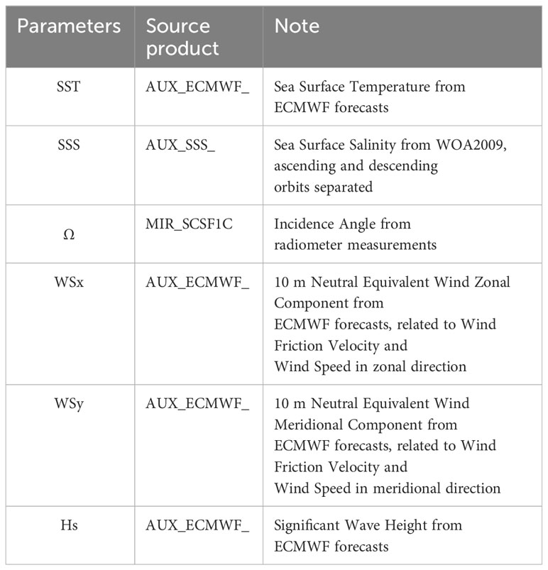
Table 3 Parameters used in constructing the SVR model.

6 Validation

6.1 Depiction in angular domain

The RFI mitigation results for co-polarization are straightforward in the angular domain, suggesting that the measured brightness temperature outliers should be pulled back to a reasonable range after the mitigation process. In Figure 4, the observed brightness temperatures for one grid point in a satellite pass are plotted, where three and four measurements are determined as being RFI contaminated for HH- and VV-polarization, respectively. Using the proposed method, these outliers are regressed to be notably close to, yet not entirely fall on the fitted polynomial, because of the different regression approaches in the detection and mitigation phases. In addition, the mitigated results are not necessarily on the same side of the fitted curve as the original contaminated measurements, such as the one for HH-polarization at the incidence angle of around 50^°. The observed measurement is much below the fitted polynomial, while the mitigated result is slightly above it.

Figure 4

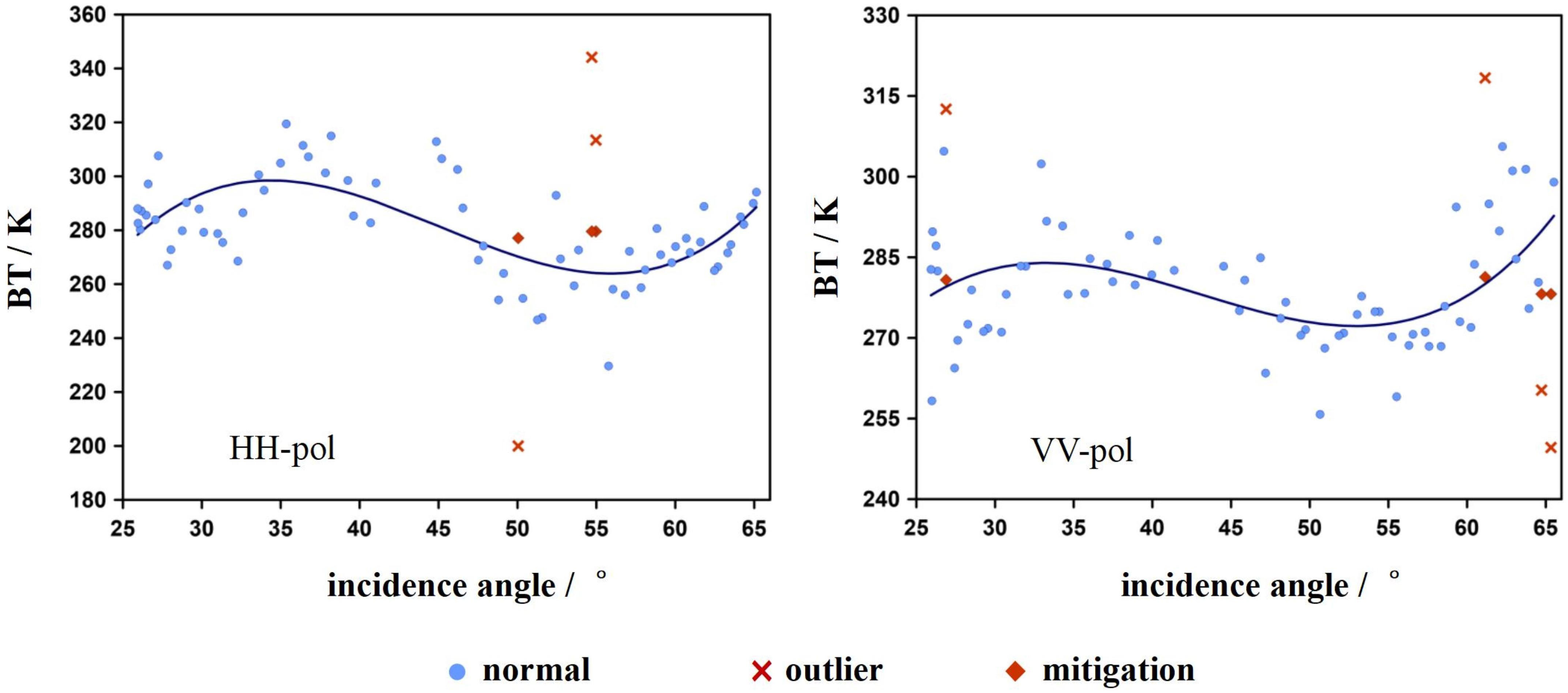
Figure 4 RFI mitigation results in the angular domain. For one grid point (Grid Point ID 4065028) in a satellite descending pass (July 1st, 2018, 09:53:20 to 10:46:34). The left and the right sub-figures are for HH- and VV-polarization, respectively. Blue circles are brightness temperature measurements in the normal range, from which the blue line representing the third-order polynomial is constructed. Red crosses are outliers, and red diamonds are their corresponding mitigation results using the SVR regression.

6.2 Depiction in space domain

Figures 5–7 displays the brightness temperature maps of three SMOS snapshots before and after the RFI mitigation process. These three snapshots are spatially close and are selected to comprise all polarization modes. The terrestrial area in the mitigated results is blanked out since it is outside the scope of this study, while in the original observed maps are retained to show the exact location of RFI emission sources on lands.

Figure 5

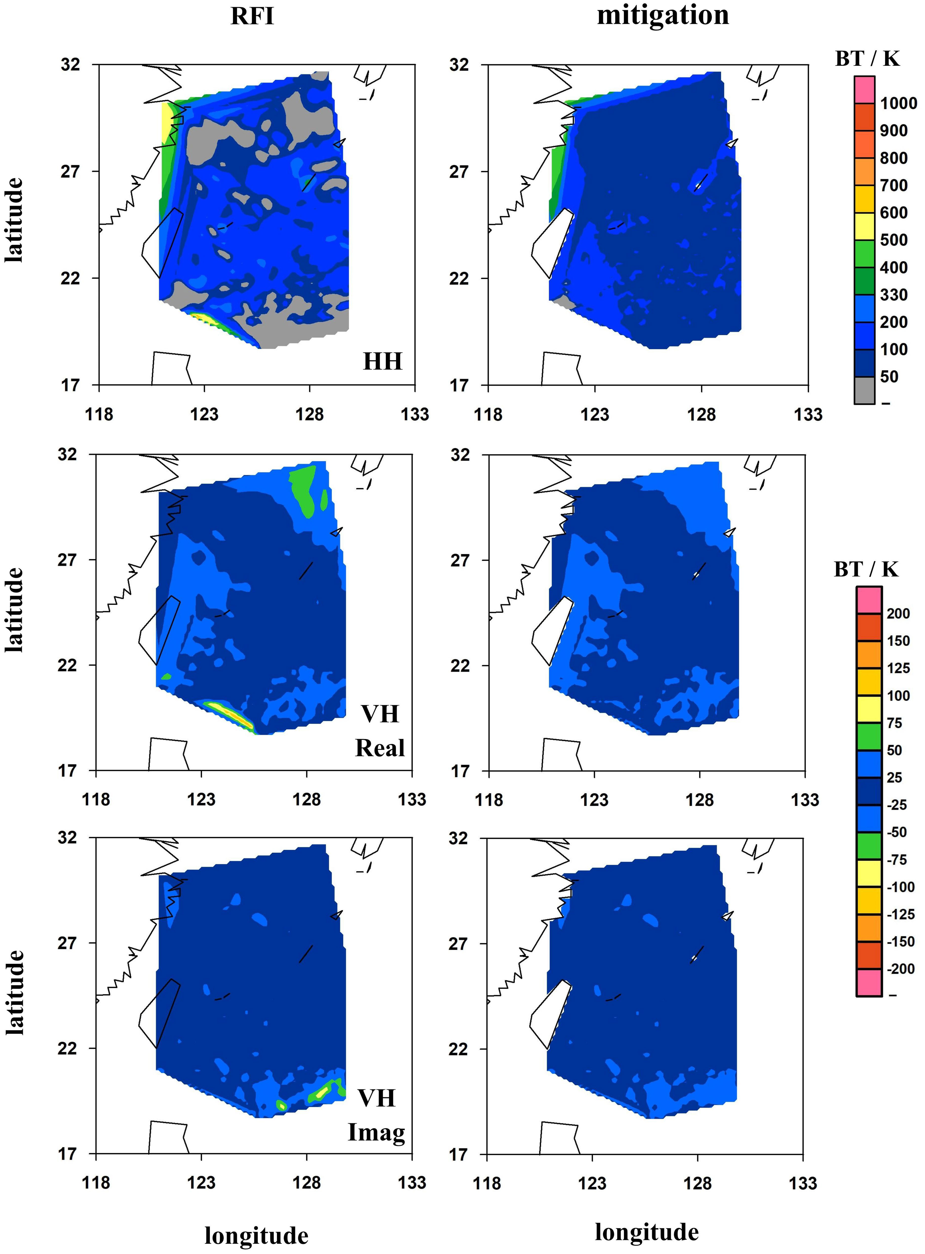
Figure 5 RFI mitigation results in the space domain. For Snapshot ID 455250354 in a satellite ascending pass (July 1st, 2018, 20:43:45 to 21:37:03), the polarization modes include HH- and VH- polarization. Sub-figures on the left and right columns are the satellite observed brightness temperatures and the mitigated results, respectively.

Figure 6

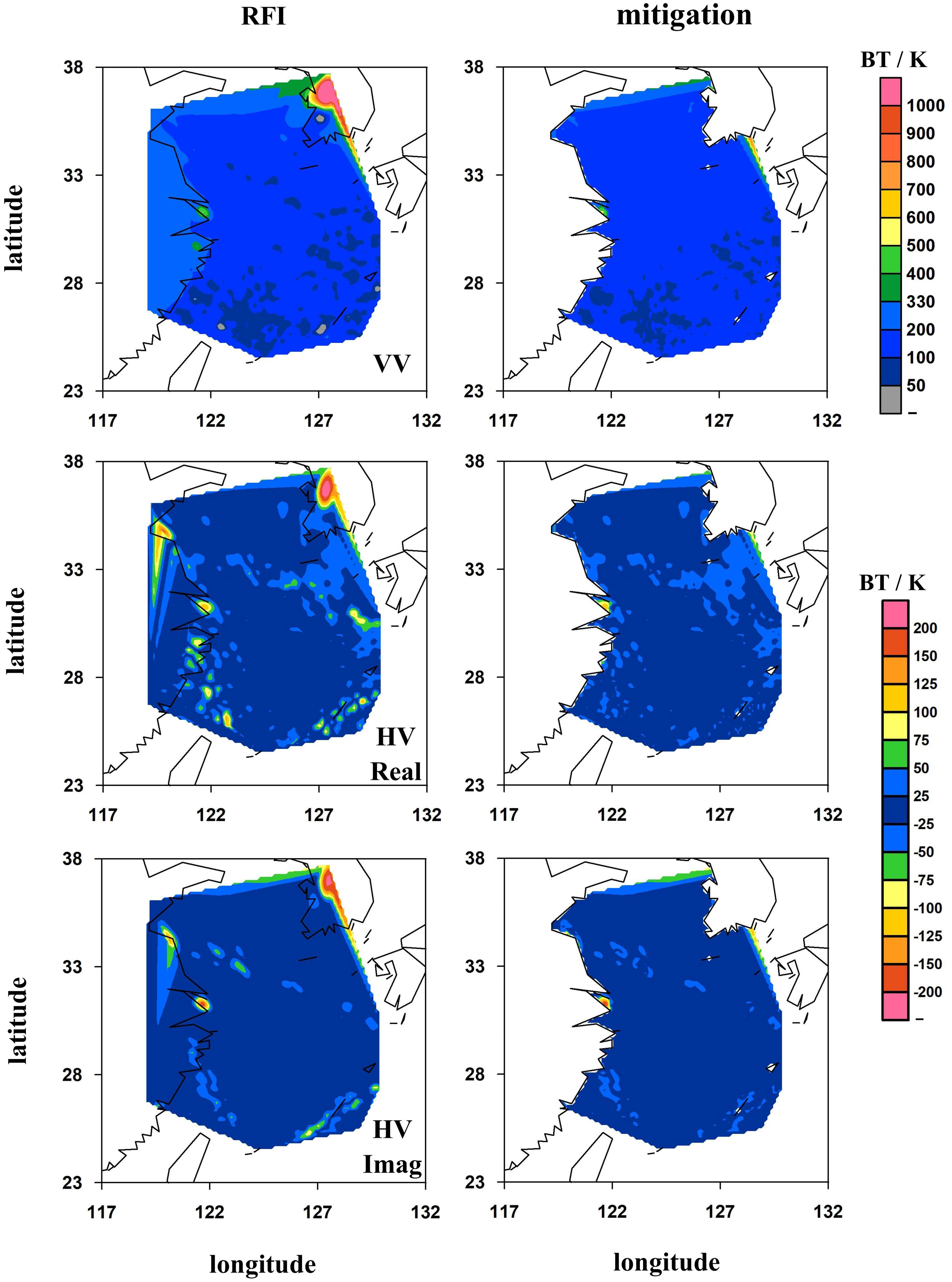
Figure 6 RFI mitigation results in the space domain. For Snapshot ID 455250453 in a satellite ascending pass (July 1st, 2018, 20:43:45 to 21:37:03), the polarization modes include VV- and HV- polarization. Sub-figures on the left and right columns are the satellite observed brightness temperatures and the mitigated results, respectively.

Figure 7

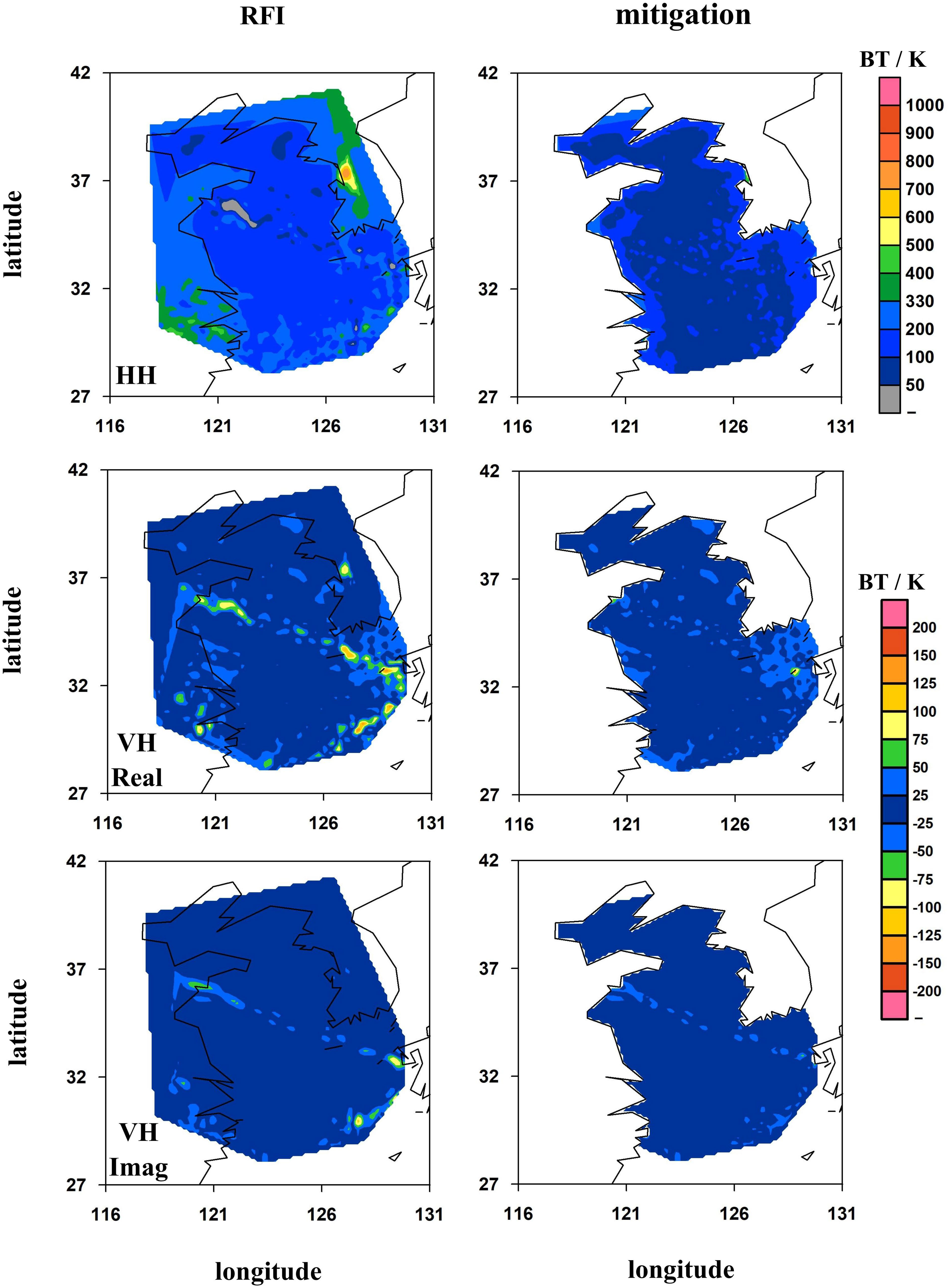
Figure 7 RFI mitigation results in the space domain. For Snapshot ID 455250513 in a satellite ascending pass (July 1st, 2018, 20:43:45 to 21:37:03), the polarization modes include HH- and VH- polarization. Sub-figures on the left and right columns are the satellite observed brightness temperatures and the mitigated results, respectively.

For the first snapshot (ID 455250354, Figure 5), when operated in HH-polarization, a number of observed brightness temperatures are less than 50 K and even negative, instead of positive, as differentiated in gray color. This is obviously illegitimate and is likely the effect of the side lobes of the intermittent RFI emissions, that only occur in some intervals of the switching sequence (Camps et al., 2011). As for the exact RFI source location, the coastal area of Zhejiang province is noteworthy and its mitigation is encouraging as the negative values are well eliminated, despite that a few of them are still visible in the lower left and that some high brightness temperatures remain in the upper left of the snapshot, indicating that the measurements for these grid points are too scarce (< 6) for the proposed algorithm to be implemented. However, this is understandable considering these grids are near the boundary of the discussed satellite pass, where the measurements are inherently much less than in the center of the track. In the case of the VH-polarization, the mitigation performance is commendable when compared with the original measurements in that the abnormally high values are successfully suppressed.

For the second snapshot ((ID 455250453, Figure 6), the mitigation results are also promising. Although along coastlines such as Hangzhou Bay, Zhejiang Province, some severe RFI impacts are inevitably retained, primarily because the seaboard itself is contaminated so hard, and partly for the same reason as in the first snapshot, that the area happens to be on the boundary of the discussed satellite pass. In any case, the consequence is that the remaining measurements are insufficient to construct a regression for RFI mitigation. Fortunately, this does not detract from the fact that RFI impacts on the majority of oceans have indeed been significantly attenuated, both in terms of co-polarization and cross-polarization.

For the third snapshot (ID 455250513, Figure 7), the situation is similar to that of the second snapshot, the RFI effects have been significantly suppressed on oceans. One notable feature of RFI impacts presented in cross-polarization, which also appears in the second snapshot, is the radiation pattern of the contamination signature, like the abnormal “line” from areas of Jiaozhou Bay, Shandong province and Haizhou Bay, Jiangsu province, extends all the way to southern Japan. This is a typical pattern of side lodes or “tails” of the impulse response of the RFI emission. In other words, this radiated contamination “line” is caused by the same RFI source that is possibly located in the coastal region of Shandong and Jiangsu province, China. After mitigation, the apparent outliers on this “line”, although still visible, have been successfully smoothed to the normal range and could be considered free of RFI contamination.

6.3 Standard deviation over the ocean

It is intrinsic that the standard deviation of brightness temperature measurements in one snapshot should not be too high, and that over adjacent snapshots should be relatively close, since the sea surface is a rather homogeneous radiating body, if there is no RFI present in the region. Figure 8 shows the variation of standard deviations of all snapshots containing a certain grid point, that is to say, these snapshots are not too far apart geographically. However, before RFI mitigation, as shown in blue filling of Figure 8, some peaks arise both in co-polarization and in cross-polarization real and imaginary parts, signifying the impacts of RFI contamination. After the mitigation process, these peaks are successfully reduced and smoothed to a reasonable range as expected. This smoothing should not just brutally flatten the curve but still follow the original trend as Figure 8 depicts. Moreover, it can be seen that some of the standard deviations after the mitigation are still at the same level as the original measurements, which suggests that these snapshots are initially clean from RFI impacts and therefore remain unchanged during the mitigation process. Also note that the Y-axis of the cross-polarization imaginary part is narrower than the others, indicating the relatively insensitive of the fourth Stokes parameter A4 to RFI contamination, yet the peaks on it can also be diminished successfully.

Figure 8

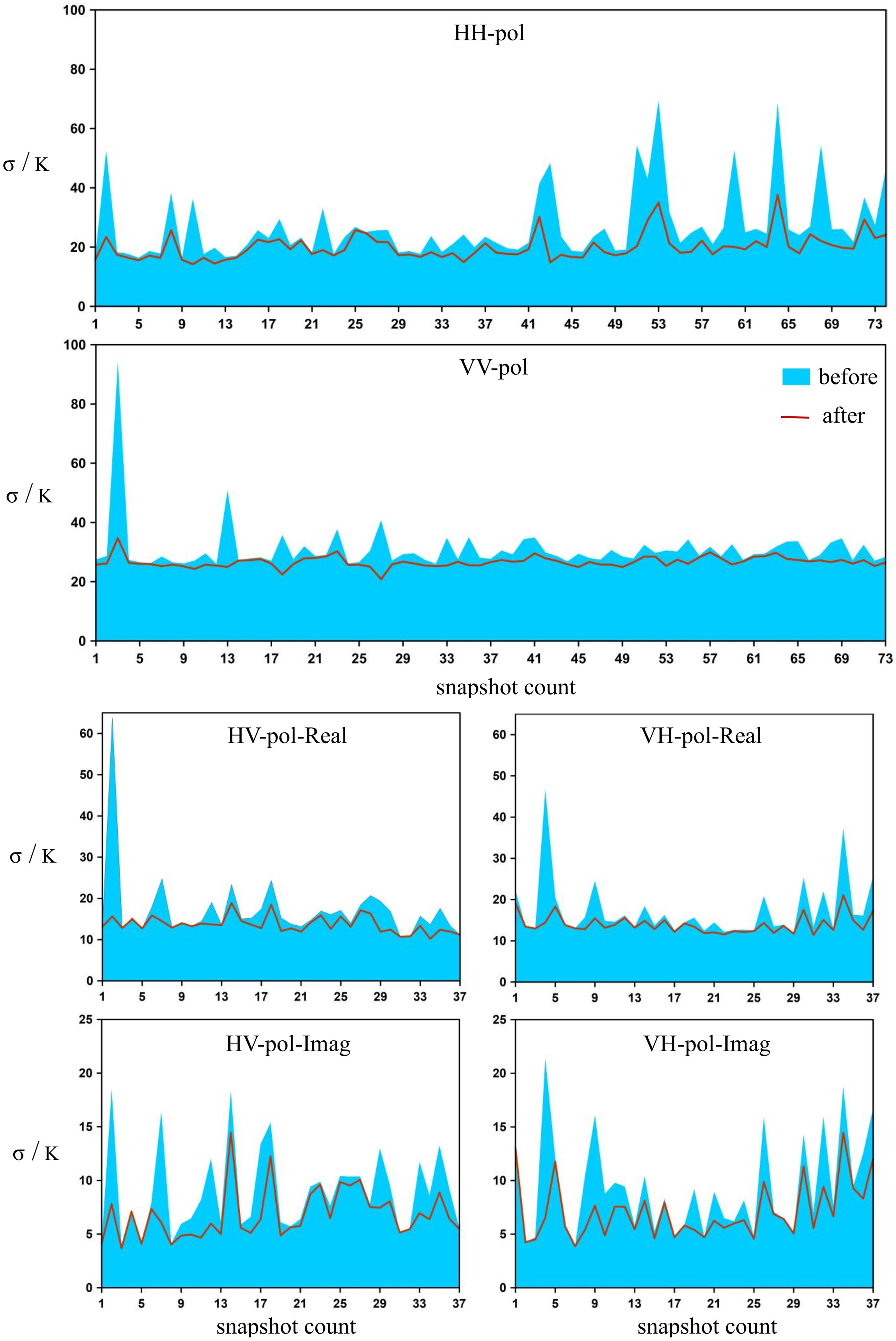
Figure 8 Standard deviations of brightness temperatures for all snapshots containing a grid point. For one grid point (Grid Point ID 4093241) in a satellite ascending pass (July 1st, 2018, 20:43:45 to 21:37:03), there are a total of 147 snapshots containing it, each of which may in one or two polarization, resulting in 74 HH-polarization, 73 VV-polarization, 37 HV-polarization and 37 VH-polarization snapshots, respectively. The blue filling is the standard deviation of the observed brightness temperatures in the snapshot, and the red line is of the mitigated results.

6.4 Retrieved SSS

Perhaps the most intuitive and convincing evidence for the proposed method is to see after the brightness temperatures have been mitigated from RFI impacts, whether the retrieved SSS actually recovers some areas that are unattainable with the current SMOS OSUDP2 SSS products. To inspect this, the SMOS L2OS Operational Processor Software developed by (ARGANS, 2023a) authorized by the SMOS team is utilized to implement a formal retrieval procedure from the altered brightness temperatures to the SSS data. Although our method is viable for measurements of any SAIR instrument, the current L2OS version 6.62 software is not compatible with the latest SMOS SCSF1C version 724 products, so the retrieval procedure is carried out on several SCSF1C version 620 products stored previously.

SMOS SCSF1C product is in a format of combined XML schema and binary Data Block, with different data types for each record. With the help of the SMOS Data Viewer software (SMOS, 2023b) and the product specification document (SMOS, 2023d), the data organization approach is carefully examined to ensure the altered brightness temperatures can be written back to the SCSF1C product in compliance with the original format. Then the ocean salinity retrieval procedure is executed separately from the rewritten SCSF1C brightness temperatures to the new OSUDP2 SSS, and from the original SCSF1C brightness temperatures to the old OSUDP2 SSS, by the L2OS software restricted on the 64 bits LINUX Operating System. During this process, Sea Surface Salinity Anomaly is automatically calculated with reference to the WOA2009 SSS (Sea Surface Salinity Anomaly = retrieved SSS - WOA2009 SSS) and written into the SSS_anom fields of the OSUDP2 products. Figure 9 briefly depicts the process.

Figure 9

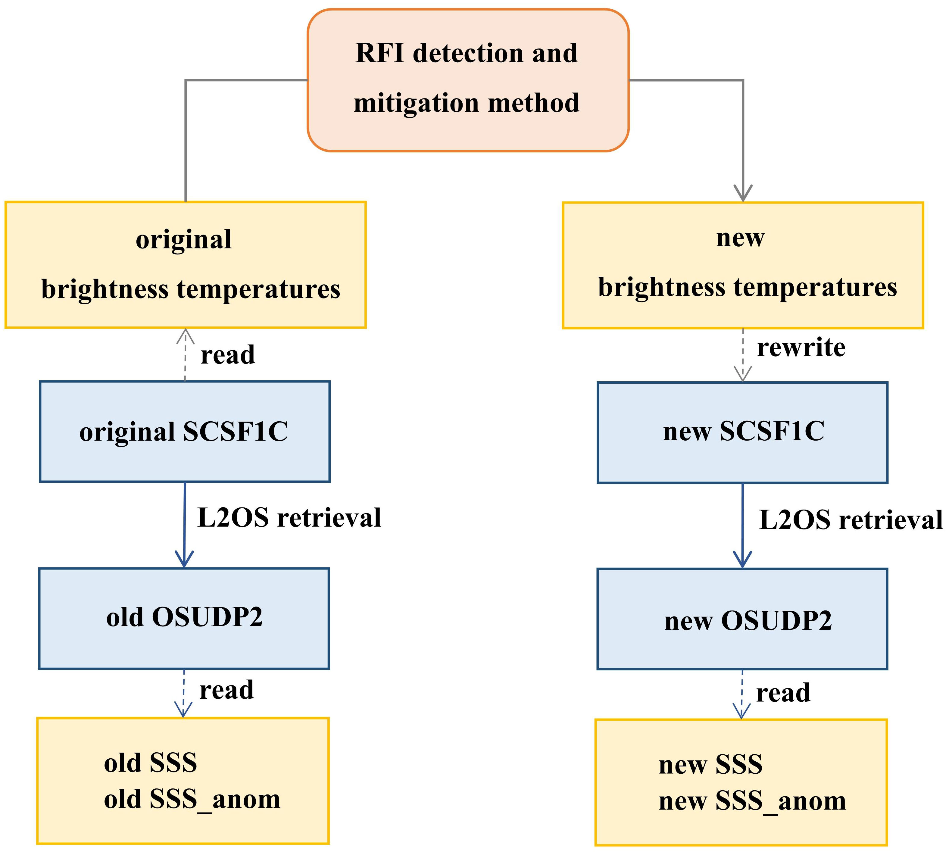
Figure 9 Ocean salinity map generation process. From the original SCSF1C product can the original brightness temperatures be read out. Using the proposed RFI detection and mitigation method, the original brightness temperatures are changed to new brightness temperatures, which should be free of RFI contamination. Then, these new brightness temperatures are rewritten into the new SCSF1C product, thus completing the preparation phase before the SSS retrieval process. With the official L2OS software, the new SCSF1C product will retrieve the new OSUDP2 product, and the original SCSF1C product generates the old OSUDP2 product. Finally, the SSS and SSS anom fields are read out from the new and old OSUDP2 products.

Figure 10 shows the new OSUDP2 SSS retrieved from our rewritten SCSF1C, the old OSUDP2 SSS retrieved from the original SCSF1C, and their SSS_anom from the WOA2009 SSS, respectively. It is apparent that the new OSUDP2 has achieved the re-acquisition of SSS fields in some places inaccessible with the old OSUDP2 products. In addition, from the SSS_anom fields, acceptable errors can be obtained for these re-gained SSS compared to WOA2009 SSS, with the exception of the coastlines, where the errors are extremely high. The proposed method fails in seaboard mainly because it itself as the RFI emission source can hardly have enough valid measurements for correction. Therefore, the ultimate solution to RFI contamination, either on oceans or continents, is to shut down the emission sources once and for all. Nevertheless, even in adjacent oceans not far from the mainland like the East China Sea and South China Sea, the proposed method helps reconstruct the SSS field, confirming its effectiveness in RFI mitigation.

Figure 10

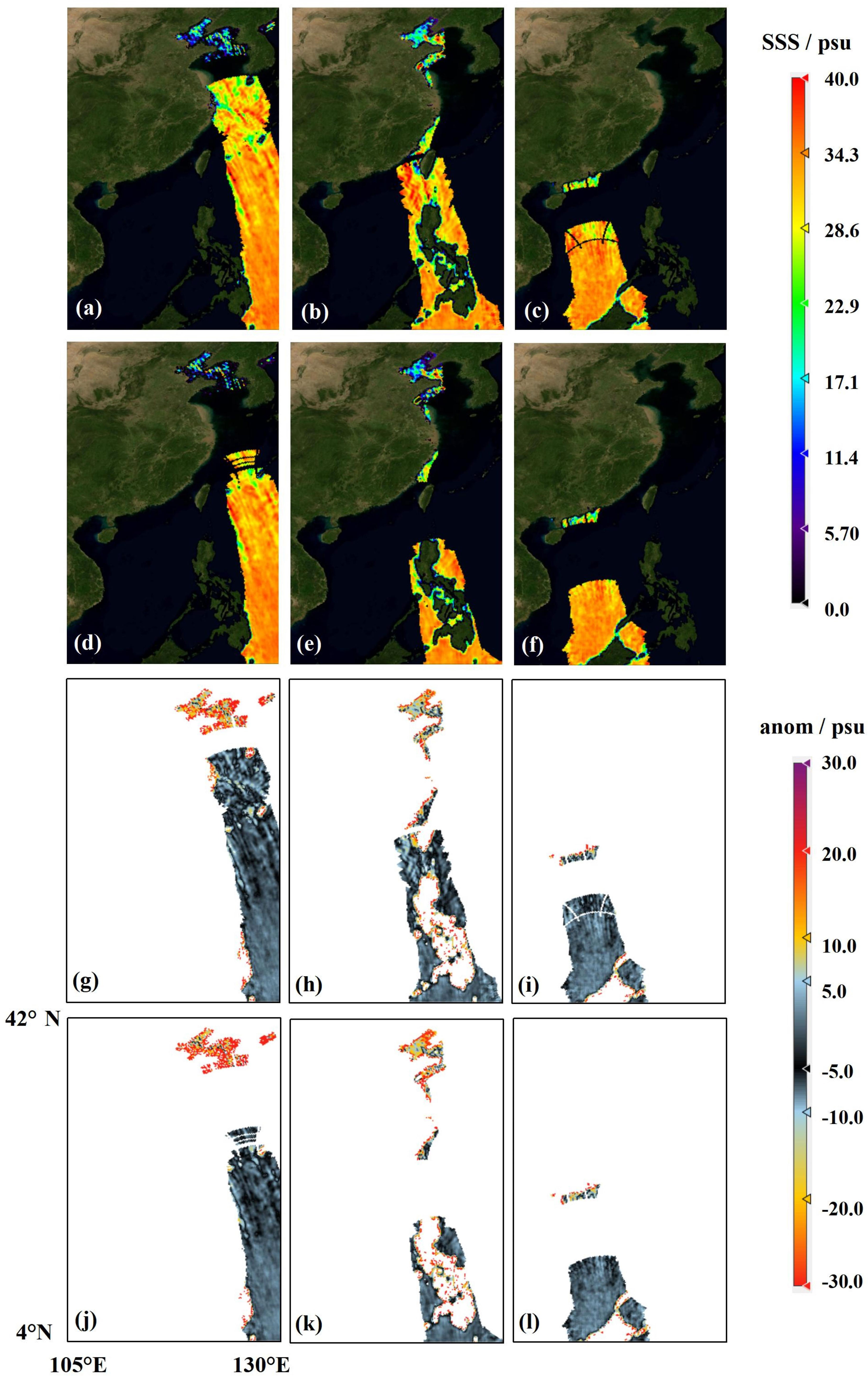
Figure 10 Retrieved SSS from new brightness temperatures after RFI mitigation, and that from original brightness temperatures, as well as their differences from WOA2009 SSS. Rows from top to bottom are: (A–C) retrieved SSS from new brightness temperatures after RFI mitigation by the proposed method; (D–F) retrieved SSS from original brightness temperatures; (G–I) SSS_anom between (A–C) and WOA2009 SSS, respectively; (J–L) SSS_anom between (D–F) and WOA2009 SSS, respectively. Columns from left to right, the corresponding satellite passes are taken from: (A, D, G, J) July 1st, 2018, 20:43:45 to 21:37:03; (B, E, H, K) July 8th, 2018, 21:11:18 to 22:04:38; (C, F, I, L) July 20th, 2018, 21:44:14 to 22:37:35. All sub-figures are zoomed in to only the region of interest (4^°N −42^°N,105^°E−130^°E) and directly exported from the SNAP-SMOS Toolbox (ESA/ESRIN, 2023).

7 Conclusion

Satellite remote sensing by 2D SAIR instrument is a new trend in acquiring Sea Surface Salinity data, with the first realization of MIRAS aboard SMOS mission and further investigation on IMR of the Chinese Ocean Salinity Satellite under development. However, the allocated frequency of the L-band for SSS observation is subject to Radio Frequency Interference from a large number of illegal emitters on lands, whose impacts may reach the nearby oceans through side lobes of the impulse response, which severely contaminate sea surface brightness temperature measurements, leading to unavailable or inaccurate SSS fields. Under the circumstances, this study establishes a practical and feasible RFI detection and mitigation method on the foundation of the radiation theory and the specialty of the SAIR instrument, combined with a simple machine learning technique of the SVR model. The goal is to eliminate or attenuate RFI impacts on measured brightness temperatures and therefore improve the quality of the retrieved SSS products, regardless of the intensity, precise location, or the underlying cause of RFI emissions. The proposed method is validated on brightness temperatures in the angular and space domain, with the outliers being pulled back to the normal range. Also, the variation of standard deviations in neighboring snapshots is smoothed over the ocean after the mitigation process is implemented. Furthermore, with the official L2OS software, the retrieved SSS from the altered brightness temperatures have succeeded in re-acquiring data in some unattainable places for the current OSUDP2 SSS products, with an acceptable SSS accuracy compared to WOA2009 SSS. We hope this work could provide a practical solution to the predicament of SAIR observations, including the ongoing SMOS mission, the Chinese Ocean Salinity Satellite due in 2024, or other satellites in the future.

Data availability statement

The original contributions presented in the study are included in the article/Supplementary Material. Further inquiries can be directed to the corresponding author.

Author contributions

MX: Methodology, Validation, Writing – original draft. HL: Conceptualization, Investigation, Project administration, Writing – review & editing. XY: Conceptualization, Writing – review & editing.

Funding

The author(s) declare financial support was received for the research, authorship, and/or publication of this article. This research was supported by the National Program on Global Change and Air-Sea Interaction (Phase II)-Parameterization assessment for interactions of the ocean dynamic system.

Acknowledgments

The authors would like to thank Piesat Information Technology Co., Ltd for their valuable advice. We also gratefully acknowledge the SMOS team and European Space Agency, Centre Aval de Traitement des Donn Données SMOS, Barcelona Expert Center, for providing materials and data in this article.

Conflict of interest

The authors declare that the research was conducted in the absence of any commercial or financial relationships that could be construed as a potential conflict of interest.

Publisher’s note

All claims expressed in this article are solely those of the authors and do not necessarily represent those of their affiliated organizations, or those of the publisher, the editors and the reviewers. Any product that may be evaluated in this article, or claim that may be made by its manufacturer, is not guaranteed or endorsed by the publisher.

Supplementary material

The Supplementary Material for this article can be found online at: https://www.frontiersin.org/articles/10.3389/fmars.2023.1290383/full#supplementary-material

References

Anterrie E. (2011). On the detection and quantification of rfi in l1a signals provided by smos. IEEE Trans. Geosci. Remote Sens. 49, 76–84. doi: 10.1109/TGRS.2011.2136350

CrossRef Full Text | Google Scholar

Anterrieu E., Khazaal A., Cabot F., Kerr Y. (2016). Geolocation of rfi sources with sub-kilometric accuracy from smos interferometric data. Remote Sens. Environ. 180, 76–84.

Google Scholar

ARGANS (2023a). Smos l2 os operational processor software release document, so-rn-arg-gs-0019. Available at: https://smos.argans.co.uk/.

Google Scholar

ARGANS (2023b). Tuning l2os rfi detection, so-tn-arg-gs-0076. Available at: https://smos.argans.co.uk/.

Google Scholar

BEC (2023). The global smos sss v2.0 produced at bec is freely available through its data visualization and distribution service. Available at: http://bec.icm.csic.es/bec-ftp-service/.

Google Scholar

Brown D., Gran R., Buis A. (2015). International spacecraft carrying nasa’s aquarius ends operations - nasa. Available at: https://www.nasa.gov/press-release/international-spacecraft-carrying-nasa-s-aquarius-instrument-ends-operations/.

Google Scholar

Camps A., Gourrion J., Tarongí J. M., Gutierréz A., Barbosa J., Castro R. (2010). “Rfi analysis in smos imagery,” in 2010 IEEE International Geoscience and Remote Sensing Symposium, Honolulu, HI, USA. 2007–2010. doi: 10.1109/IGARSS.2010.5654268

CrossRef Full Text | Google Scholar

Camps A., Gourrion J., Tarongí J., Vall-llossera M., Gutierrez A., Barbosa J., et al. (2011). Radiofrequency interference detection and mitigation algorithms for synthetic aperture radiometers. Algorithms 4, 155–182. doi: 10.3390/a4030155

CrossRef Full Text | Google Scholar

Camps A., Park H., Gonzalez-Gambau V. (2014). “An imaging algorithm for synthetic aperture interferometric radiometers with built-in rfi mitigation,” in 2014 13th Specialist Meeting on Microwave Radiometry and Remote Sensing of the Environment (MicroRad), Pasadena, CA, USA. 39–43. doi: 10.1109/MicroRad.2014.6878904

CrossRef Full Text | Google Scholar

Castro R., Gutierrez A., Barbosa J. (2013). A first set of techniques to detect radio frequency interferences and mitigate their impact on smos data. IEEE Trans. Geosci. Remote Sens. 50, 1440–1447. doi: 10.1109/TGRS.2011.2179304

CrossRef Full Text | Google Scholar

CATDS (2023). Catds-pdc l3os 3g - debiased gaussian average daily salinity field product from smos satellite. doi: 10.12770/9c97fb5c-d7d5-4bc2-a5c7-57944026cd60

CrossRef Full Text | Google Scholar

Chang C., Lin C. (2011). Libsvm: a library for support vector machines. ACM Trans. Intelligent Syst. Technol. 2, 1–27. doi: 10.1145/1961189.1961199

CrossRef Full Text | Google Scholar

Corbella I., Torres F., Camps A., Duffo N., Vall-llossera M. (2009). Brightness-temperature retrieval methods in synthetic aperture radiometers. IEEE Trans. Geosci. Remote Sens. 47, 285–294. doi: 10.1109/TGRS.2008.2002911

CrossRef Full Text | Google Scholar

Cortes C., Vapnik V. (1995). Support-vector networks. Mach. Learn. 20, 273–297. doi: 10.1007/BF00994018

CrossRef Full Text | Google Scholar

Daganzo-Eusebio E., Oliva R., Kerr Y. H., Nieto S., Richaume P., Mecklenburg S. M. (2013). Smos radiometer in the 1400-1427-mhz passive band: impact of the rfi environment and approach to its mitigation and cancellation. IEEE Trans. Geosci. Remote Sens. 51, 4999–5007. doi: 10.1109/TGRS.2013.2259179

CrossRef Full Text | Google Scholar

Drucker H., Burges C., Kaufman L., Smola A., V Vapnik V. (1997). Support vector regression machines. Adv. Neural Inf. Process. Syst. 9, 155–161.

Google Scholar

Entekhabi D., Njoku E., O’Neill P. (2009). “The soil moisture active and passive mission (smap): science and applications,” in 2009 IEEE Radar Conference, Pasadena, CA, USA. 1–3. doi: 10.1109/RADAR.2009.4977030

CrossRef Full Text | Google Scholar

ESA/ESRIN (2023). Smos toolbox. Available at: https://earth.esa.int/eogateway/tools/smos-toolbox.

Google Scholar

Font J., Kerr Y. H., Srokosz M. A., Etcheto J., Lagerloef G. S., Camps A., et al. (2001). “Smos: a satellite mission to measure ocean surface salinity,” in Atmospheric Propagation, Adaptive Systems, and Laser Radar Technology for Remote Sensing. Eds. Gonglewski J. D., Kamerman G. W., Kohnle A., Schreiber U., Werner C. H. (The name of the publisher), 207–214. doi: 10.1117/12.413825

CrossRef Full Text | Google Scholar

Jin R., Lu H., Chen L., Gao Y., Li Q. (2022a). Low- and moderate-level rfi detection using point-source ripple for synthetic aperture interferomentric radiometer. IEEE Trans. Geosci. Remote Sens. 60, 1–13. doi: 10.1109/TGRS.2022.3168984

CrossRef Full Text | Google Scholar

Jin R., Wu L., Li Q., Lu H., Feng L. (2022b). Geolocation of rfis by multiple snapshot difference method for synthetic aperture interferomentric radiometer. IEEE Trans. Geosci. Remote Sens. 60, 1–12. doi: 10.1109/TGRS.2020.3045088

CrossRef Full Text | Google Scholar

Johnson J. T., Aksoy M. (2011). “Studies of radio frequency interference in smos observations,” in 2011 IEEE International Geoscience and Remote Sensing Symposium, Vancouver, BC, Canada. 4210–4212. doi: 10.1109/IGARSS.2011.6050159

CrossRef Full Text | Google Scholar

Klein L., Swift C. (1977). An improved model for the dielectric constant of sea water at microwave frequencies. IEEE Trans. Antennas Propagation 25, 104–111. doi: 10.1109/TAP.1977

CrossRef Full Text | Google Scholar

Kristensen S. S., Balling J. E., Skou N., Søbjærg S. S. (2012). “Rfi detection in smos data using 3rd and 4th stokes parameters,” in 2012 12th Specialist Meeting on Microwave Radiometry and Remote Sensing of the Environment (MicroRad), Rome, Italy. 1–4. doi: 10.1109/MicroRad.2012.6185254

CrossRef Full Text | Google Scholar

Lagerloef G., Colomb F. R., LeVine D., Wentz F., Yueh S., Ruf C., et al. (2008). The aquarius/sac-d mission: designed to meet the salinity remote-sensing challenge. Oceanography 21, 68–81. doi: 10.5670/oceanog.2008.68

CrossRef Full Text | Google Scholar

Levine D. M., Good J. C. (1983). Aperture synthesis for microwave radiometers in space, technical memorandum tm-85033 (Greenbelt, Maryland: NASA Goddard Space Flight Center).

Google Scholar

Li Y., Yin X., Zhou W., Lin M., Liu H., Li Y. (2022). Performance simulation of the payload imr and micap onboard the chinese ocean salinity satellite. IEEE Trans. Geosci. Remote Sens. 60, 1–16. doi: 10.1109/TGRS.2021.3111026

CrossRef Full Text | Google Scholar

Li C., Zhao H., Li H., Lv K. (2016). Statistical models of sea surface salinity in the south China sea based on smos satellite data. IEEE J. Selected Topics Appl. Earth Observations Remote Sens. 9, 2658–2664. doi: 10.1109/JSTARS.2016.2537318

CrossRef Full Text | Google Scholar

Martin-Neira M., Ribo S., Martin-Polegre A. J. (2002). Polarimetric mode of miras. IEEE Trans. Geosci. Remote Sens. 40, 1755–1768. doi: 10.1109/TGRS.2002.802489

CrossRef Full Text | Google Scholar

McMullan K. D., Brown M. A., Martin-Neira M., Rits W., Ekholm S., Marti J., et al. (2008). “Smos: the payload,” in IEEE Transactions on Geoscience and Remote Sensing, Vol. 46. 594–605. doi: 10.1109/TGRS.2007

CrossRef Full Text | Google Scholar

Misra S., Ruf C. S. (2012). Analysis of radio frequency interference detection algorithms in the angular domain for smos. IEEE Trans. Geosci. Remote Sens. 50, 1448–1457. doi: 10.1109/TGRS.2011.2176949

CrossRef Full Text | Google Scholar

Oliva R., Daganzo E., Kerr Y. H., Mecklenburg S., Nieto S., Richaume P., et al. (2012). Smos radio frequency interference scenario: status and actions taken to improve the rfi environment in the 1400-1427-mhz passive band. IEEE Trans. Geosci. Remote Sens. 50, 1427–1439. doi: 10.1109/TGRS.2012.2182775

CrossRef Full Text | Google Scholar

Oliva R., Daganzo E., Richaume P., Kerr Y., Cabot F., Soldo Y., et al. (2016). Status of radio frequency interference (rfi) in the 1400-1427 mhz passive band based on six years of smos mission. Remote Sens. Environ. 180, 64–75. doi: 10.1016/j.rse.2016.01.013

CrossRef Full Text | Google Scholar

Oliva R., Nieto S., Félix-Redondo F. (2013). Rfi detection algorithm: accurate geolocation of the interfering sources in smos images. IEEE Trans. Geosci. Remote Sens. 51, 4993–4998. doi: 10.1109/TGRS.2013.2262721

CrossRef Full Text | Google Scholar

Park H., González-Gambau V., Camps A., Vall-llossera M. (2016). Improved music-based smos rfi sources detection and geolocation algorithm. IEEE Trans. Geosci. Remote Sens. 54, 1311–1322. doi: 10.1109/TGRS.2015.2477435

CrossRef Full Text | Google Scholar

Skou N., Balling J. E., Søbjærg S. S., Kristensen S. S. (2010). “Surveys and analysis of rfi in the smos context,” in 2010 IEEE International Geoscience and Remote Sensing Symposium, Honolulu, HI, USA. 2011–2014. doi: 10.1109/IGARSS.2010.5649838

CrossRef Full Text | Google Scholar

SMOS (2023a). Esa smos online dissemination. Available at: https://smos-diss.eo.esa.int/oads/access/collection.

Google Scholar

SMOS (2023b). Smos data viewer. Available at: https://earth.esa.int/eogateway/tools/smos-data-viewer.

Google Scholar

SMOS (2023c). Smos l2 os algorithm theoretical baseline document (atbd) so-tn-arg-gs-0007. Available at: https://earth.esa.int/eogateway/documents/20142/37627/SMOS-L2OS-ATBD.pdf.

Google Scholar

SMOS (2023d). Smos level1 and auxiliary data products specifications, so-tn-idr-gs-0005. Available at: https://earth.esa.int/eogateway/catalog/smos-science-products.

Google Scholar

Soldo Y., Cabot F., Khazaal A., Miernecki M., Słomińska E., Kerr R. F. Y. H. (2015). Localization of rfi sources for the smos mission: a means for assessing smos pointing performance. IEEE J. Selected Topics Appl. Earth Observations Remote Sens. 8, 617–627. doi: 10.1109/JSTARS

CrossRef Full Text | Google Scholar

Soldo Y., Khazaal A., Cabot F., Richaume P., Anterrieu E., Kerr Y. (2014). Mitigation of rfis for smos: a distributed approach. IEEE Trans. Geosci. Remote Sens. 52, 7470–7479. doi: 10.1109/TGRS.2014.2312988

CrossRef Full Text | Google Scholar

Vapnik V. N., Lerner A. (1963). Pattern recognition using generalized portrait method. Automation Remote Control 24, 774–780.

Google Scholar

Xu M., Li H., Chen H., Yin X. (2022). Quantitative measurement of radio frequency interference for smos mission. Remote Sens. 14. doi: 10.3390/rs14071669

CrossRef Full Text | Google Scholar

Yang P. (2023). An imaging algorithm for high-resolution imaging sonar system. Multimedia Tools Appl. doi: 10.1109/JSTARS.2016.2537318

CrossRef Full Text | Google Scholar

Zhang X., Yang P., Sun H. (2023). An omega-k algorithm for multireceiver synthetic aperture sonar. Electron. Lett. 59, 1–3. doi: 10.1049/ell2.12859

CrossRef Full Text | Google Scholar