 Maitane Pérez-Cebrecos
 Xabier Berrojalbiz1
 Urtzi Izagirre
 Irrintzi Ibarrola
- 1FEMB Research Group, Department of Genetics, Physical Anthropology and Animal Physiology, Faculty of Science and Technology, University of the Basque Country (UPV/EHU), Leioa, Spain
- 2Research Centre for Experimental Marine Biology and Biotechnology (PiE – UPV/EHU), University of the Basque Country (UPV/EHU), Plentzia, Spain
- 3BCTA Research Group, Department of Zoology and Animal Cell Biology, Faculty of Science and Technology, University of the Basque Country (UPV/EHU), Leioa, Spain
Understanding how allometric exponents vary in the different biologically determined patterns turns out to be fundamental for the development of a unifying hypothesis that intends to explain most of the variation among taxa and physiological states. The aims of this study were (i) to analyze the scaling exponents of oxygen consumption at different metabolic rates in Mytilus galloprovincialis according to different seasons, habitat, and acclimation to laboratory conditions and (ii) to examine the variation in shell morphology depending on habitat or seasonal environmental hazards. The allometric exponent for standard metabolic rate (b value) did not vary across seasons or tide level, presenting a consistent value of 0.644. However, the mass-specific standard oxygen consumption (a value), i.e. metabolic level, was lower in intertidal mussels (subtidal mussels: a = - 1.364; intertidal mussels: a = - 1.634). The allometric exponent for routine metabolic rate changed significantly with tide level: lower allometric exponents for intertidal mussels (b = 0.673) than for subtidal mussels (b = 0.871). This differential response did not change for at least two months after the environmental cue was removed. We suggest that this is the result of intertidal mussels investing fundamentally in surface-dependent organs (gill and shell), with the exception of the slightly higher values obtained in May as a likely consequence of gonadal tissue development. Subtidal mussels, on the contrary, are probably in constant demand for volume-related resources, which makes them consistently obtain an allometric exponent of around 0.87.
1 Introduction
Studying the factors that influence respiratory metabolism is essential because it can affect a wide range of activities and their interpretation at different levels of the biological hierarchy. One of the most important physiological factors affecting metabolism is body size. Within specific taxonomic groups, R –metabolic rate– often varies closely with M –body mass–, following a power function that can be described as:
where a is the scaling coefficient (or proportionality constant) and b is the scaling exponent (or logarithmic slope). This relationship has been a source of discussion considering that even though a reasonable variation both within and among taxa is acknowledged for b value, it is unknown if these variations are deviations from a general law, or whether there is no such law (Agutter and Wheatley, 2004). The so-called ‘3/4-power law’, was proposed by Kleiber (1932), who noted a value of 0.75 for the scaling exponent of birds and mammals. Hemmingsen (1960) also revealed a value of around 0.75 for a heterogeneous bunch of poikilotherms. Since then, a scaling exponent of 0.75 has been assumed for virtually all organisms (e.g., Brown et al., 2004), despite the activity or metabolic level, giving the impression of a common underlying mechanistic origin (Savage et al., 2004). However, due to the broad assumptions of the law and the ample amount of examples in which the b value deviates from 0.75 (see Glazier, 2005), it has suffered harsh criticism (e.g., Bokma, 2004; Suarez et al., 2004; Glazier, 2005; Muller-Landau et al., 2006; White et al., 2006; Glazier, 2008; Glazier, 2009; Glazier, 2010; White, 2011; Carey et al., 2013), and it seems to be no longer acceptable (Glazier, 2022b).
In the face of controversy, alternative models have been proposed to explain the variety of metabolic scaling relationships observed (reviewed in da Silva et al., 2006; O’Connor et al., 2007) often evolving towards covering theoretical models that embrace not only physical factors, but also the influence of biological regulation, various abiotic and biotic ecological factors, and evolutionary optimization (Glazier, 2022b). Although some theoretical approaches include the effects of body shape, (e.g. Hirst et al., 2014; Glazier, 2015) and cellular model of growth (e.g. Kozlowski et al., 2003; Kozlowski et al., 2020; Glazier, 2022a), to date, only the metabolic-level boundaries (MLB) hypothesis proposed by Glazier (2005; 2010, 2014) seems to explain not only most of the variation among taxa but also amongst physiological states. The MLB hypothesis describes how the observed values of b often fall between the theorized boundary values of 0.667 and 1. It explains how b varies when supply exceeds metabolic demand and when metabolic demand exceeds supply. The fluctuation of the scaling exponent between those end values might depend on metabolic rate, activity and ecological factors (Glazier, 2010). Therefore, testing is still required for some answers to be cleared up. For instance, it would be necessary to analyze which ecological factors affect not only the overall metabolic level but also the metabolic scaling exponent.
Sessile organisms, such as mussels, that inhabit temperate zones with tidal regimes may turn out to be suitable for the analysis of the aforementioned hypothesis, since although they belong to the same species, they live under different biological realities (Nicastro et al., 2010). Descendant mussels of the same spawning event can end up inhabiting either the subtidal zone or different zones along the intertidal. This vertical zonation of the mussel communities is especially relevant not only due to the different set of challenges that each zone subdues the mussels to; but also because, as long as they are sessile, they cannot move to evade the environmental stresses. In fact, high intertidal organisms are regularly exposed to large variations and steep gradients of environmental factors, such as temperature, food availability, humidity and salinity, besides the short-term and severe decrease in available oxygen that becomes more extreme higher up the shore (Mandic and Regan, 2018; McArley et al., 2019). So much so, that life in the intertidal for bivalves involves a wide range of adaptation responses such as reduced water loss, increased thermal resistance, etc. (see Leeuwis and Gamperl, 2022 for a comprehensive review).
Those same mussels affected by tide regimes are also influenced by seasons, which could also have an effect on the scaling values. Indeed, Mytilus ssp. have developed physiological regulations that modify its metabolism to cope with these ecological fluctuations (Bayne et al., 1988). Moreover, most of the measurements that aim to understand these variations are performed in the laboratory, creating the need to understand to what extent the scaling values vary when working under laboratory conditions. In addition, understanding how allometric exponents vary in those biologically determined patterns turns out to be fundamental for the standardization of growth models in bioenergetics. For the Mytilus genre, few studies have analyzed the metabolic size scaling variation (Winter, 1978; Bayne and Newell, 1983; Sprung, 1984; Hawkins et al., 1990; Arranz et al., 2016; Ibarrola et al., 2022) and even less have differentiated between standard and routine metabolic rates. This is especially relevant for M. galloprovincialis, the size standardization of which is based on values reported for related species of the same genre, mostly M. edulis (Anestis et al., 2010; Tamayo et al., 2016; Prieto et al., 2020) and occasionally M. chilensis (Sarà and Pusceddu, 2008). It has never been accomplished to our knowledge a systematic study of the metabolic size scaling of M. galloprovincialis that analyses the variation of the scaling exponents according to not only activity level but also to variable outside environmental factors.
When thorough analysis of allometric scaling is pursued in mussels, the shell dimensions need to be examined, since they are known to vary with regard to environmental factors and specific life-habitats (e.g. Steffani and Branch, 2003; Babarro and Carrington, 2011). Moreover, because the integrity of the shell determines survival, shell-form is subject to strong selection pressure, making it a fundamental evolutionary driving force. Although shells protect mussels against abiotic and biotic factors (Burnett and Belk, 2018), shell traits can also shift with body size, an endogenous parameter analyzed for some mollusks (e.g. Franz, 1993; Tokeshi et al., 2000; Alunno-Bruscia et al., 2001; Cordero-Rivera et al., 2022), but seldom considered specifically for M. galloprovincialis. Shells can also be used to explore intraspecific variations in different environments, as shell shape may also have an effect on shell performance (Fitzer et al., 2015).
In the present investigation, we analyzed the growth allometry of oxygen consumption at different metabolic rates in Mytilus galloprovincialis according to different seasons, habitat and acclimation to laboratory conditions. The influence of season and habitat on the condition index, shell density and the scaling relationship of shell dimensions was also examined. It was hypothesized that (1) scaling exponents of oxygen consumption at different metabolic rates are modified by season, habitat and acclimation time, and (2) shell-morphology differs in a way that reduces the different environmental hazards imposed by habitat or season. The findings are not only useful for mussel energetics, but provide insight into the scaling relationships of Mytilus galloprovincialis in the light of ecology, lifestyle and other extrinsic factors with reference to recent literature.
2 Materials and methods
2.1 Mussel collection and experimental setup
2.1.1 Season and tidal-regime experiment
Two samplings were made to collect M. galloprovincialis mussels from the sheltered rocky shore of Plentzia (Biscay, Spain, 43° 24’ N; 2° 56’ W) (Figure 1), coinciding with the fall (November 2021) and spring (May 2022) seasons. Water temperature was around 15.5 °C in both seasons and the phytoplankton concentration similar (Bilbao et al., 2021) In each sampling, mussels were collected at low tide (spring tides) from the intertidal (n = 30) and subtidal (n = 30) tide zones, covering the broadest size-range possible: 21.6 – 67.0 mm and 22.4 – 65 mm for the intertidal and subtidal tide regimes in November; 20.6 – 68.3 mm and 21.8 – 66.0 mm for the intertidal and subtidal mussels in May. Therefore, four different experimental groups emerge from the combination of the tidal regime (subtidal –S– vs. intertidal –I–) and sampling date (November –N– vs. May –M–): SN, IN, SM and IM.
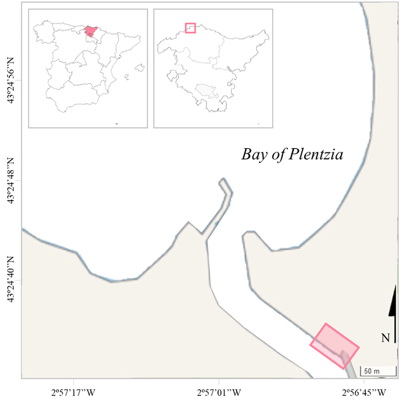
Figure 1 Sampling point in the Bay of Plentzia in Biscay (North of Spain).
Mussels were transferred to the laboratory in air-exposed wet containers. On both occasions, the procedure followed identical protocols: intertidal and subtidal mussels were placed in two different tanks (50 L) at constant seawater salinity (33 PSU) and temperature (16 °C). The next day upon arrival, the routine oxygen consumption of each individual was measured, while the standard oxygen consumption was recorded after 7 days of fasting. This period was established to be sufficient for mussels to minimize any energy cost derived from digestion processes (Prieto et al., 2018).
2.1.2 Acclimation experiment
To understand the effects that acclimation to laboratory conditions might have on the metabolism of both tidal regimes, all mussels collected in November were kept in the laboratory for a period of 2 months individualized in independent chambers. Two tanks (50 L) were used for subtidal and intertidal mussels, respectively, maintained under constant seawater salinity (33 PSU) and temperature (16 °C). The seawater was pump directly from a 12 000 L reservoir of natural seawater that is filtered through a biological filter and three subsequent fiberglass filters (100, 10 and 1 µm) before going into the recirculating water system in the laboratory. Constant food was supplied in the form of a combination of own-cultured Isochrysis galbana strain BMCC1 microalgae (Basque Microalgae Culture Collection from University of the Basque Country), and a commercial mixture (Shellfish Diet 1800®) of five marine microalgae (Isochrysis sp., Pavlova sp., Tetraselmis sp., Thalassiosira weissflogii and Thalassiosira pseudonana) constantly dosed at 20000 part · mL−1. The concentration was kept stable by frequently checking with a Coulter Multisizer 3 and homogeneity ensured with air circulation. The tanks were cleaned and seawater renewed twice a week. No mortality events were recorded during the acclimation period. After the 2-month acclimation period to continuous immersion and feeding in the laboratory, routine and standard metabolic rates were again measured. For each tidal regime, two different data sets were obtained: an initial determination corresponding to the field conditions (F) and a final determination after maintenance in the laboratory (L). Consequently, four different experimental groups were obtained in this second experiment: SF, IF, SL, and IL.
2.2 Oxygen consumption
2.2.1 Routine oxygen consumption (VO2R: mL O2·h-1)
Mussels were introduced into chambers ranging from 50 to 250 ml (according to mussel size) sealed with LDO oxygen probes connected to oxymeters (HATCH HQ40d) for the determination of routine oxygen consumption. The oxygen consumption rates were calculated from the decrease in oxygen concentration in the chambers recorded during 3-4 h, or until the values decreased 20-30% of the initial baseline, every 5-10 minutes. A control chamber was used to check the stability of the oxygen concentration.
2.2.2 Standard oxygen consumption (VO2S: mL O2 · h-1)
Standard oxygen consumption was recorded likewise, except for the 7-day fasting period in which mussels were subdued before measurements were made.
2.3 Gill surface area (GA: mm2 · g-1)
Gill surface-area measurements were only recorded for the mussels collected in May, as the mussels collected in November may not reflect field values after two months of acclimation in the laboratory. After the physiological experiments were concluded, all individuals were carefully dissected. A photograph of the internal tissues was taken with a digital camera and the surface-area of the gills of each individual was calculated using ImageJ software (Abràmoff et al., 2004). A rule was placed next to the mussel when taking the photograph for size correction. The data shown correspond to one side of the demibranch.
2.4 Shell dimensions
Biometry and shell surface-area were calculated for all 30 mussels of each tidal regime in both experiments. In the case of the acclimation experiment, both measurements were taken on arrival in the laboratory and after 2 months of maintenance. The anterior-posterior (length), dorso-ventral (height) and lateral axis (width) of the shell were measured to the nearest 0.01 mm using digital dial calipers. The shell surface-area (mm2) was obtained applying a formula resembling an ellipsoid-like shape proposed by Reimer and Tedengren, 1996:
where L, H and W are respectively the length (mm), width (mm) and height (mm).
2.5 Condition index
After both samplings, once physiological measurements were completed, the whole flesh of each animal was dissected and desiccated (24 hrs. 100 °C) to obtain the flesh dry weight (FDW). The dry weight of the shell (SDW: mg) was obtained after the flesh residues were carefully removed from the surface of the completely air-dried shell. The shells were weighed on a 0.01 mg accuracy balance, just as the live weight of the entire animal. Condition index was computed according to Davenport and Chen (1987):
where TDW represents the total dry weight of the mussel computed as FDW + SDW.
2.6 Statistical analysis
Data were evaluated for normality and homoscedasticity using Shapiro-Wilk and Levene tests, respectively, prior to data analysis. Normal distribution of the residuals was checked by Normal P-P plots and the independence of the observations tested by Durbin-Watson tests.
Linear ordinary least squares regression analyzes were performed to determine the values of the scaling exponents (b) and the coefficients (a) for each regression. Regressions were computed with log-transformed data of routine and standard oxygen consumption (VO2R and VO2S), live weight, gill surface area shell length, shell surface-area and shell dry weight. Not-logarithmically transformed data of shell width, shell height and shell length were also fitted to linear regressions. Significant differences in scaling exponents and coefficients between regressions corresponding to each experimental group were tested using covariance procedures (ANCOVA) described by Zar (1999); briefly, if the null hypothesis (H0: equal slopes b1 = b2 = b3… = bk) was rejected, multiple comparison t-test was performed to determine the significant differences between each pair of slopes. If H0 was accepted, a common slope (bc) was computed and the null hypothesis of equal intercepts (a1 = a2 = a3… = ak) was subsequently tested. If intercepts were not different, a common intercept (ac) and common regression were computed. Multiple comparison t-test was performed to determine the significant differences between each pair of elevations, in case they were different.
Data resulting from each experiment was also assessed by multiple regression analysis (after observation independence and normality of residuals were checked) to sequentially identify the explanatory variables that were most closely associated with routine oxygen consumption and standard oxygen consumption (dependent variables). For the seasonality experiment, the explanatory variables were live weight (numeric), season (dummy variable; May = 0, November = 1), tide (dummy variable; subtidal = 0, intertidal = 1), 2-way interactions (live weight x season; live weight x tide; season x tide) and 3-way interaction. For the acclimation experiment, the explanatory variables were live weight (numeric), time (dummy variable; Field = 0, Laboratory = 1), tide (dummy variable; subtidal = 0, intertidal = 1), 2-way interactions (live weight x time; live weight x tide; time x tide) and 3-way interaction.
The effect of season and tide factors on shell surface-area and condition index was analyzed with two-way factor ANOVA. Statistical analyzes were performed using IBM SPSS Statistics for Windows, Version 28.0 (IBM Corp, 2021).
3 Results
3.1 Season and tidal-regime experiment
3.1.1 Routine oxygen consumption (VO2R)
The data of routine oxygen consumption for each experimental group plotted as a function of their respective live weight can be found in Figure 2A. The resulting equations are summarized in Figure 2A on the top right. Statistical comparisons between the four regression lines showed that the slopes differed from each other (Figure 2A). The allometric exponent of the subtidal mussels was consistently higher than the allometric exponent of the intertidal ones, notwithstanding the month. However, the slope of the intertidal population in November was significantly the lowest compared to the other three. The general equation relating routine oxygen consumption with live weight (W) and tide in the multiple regression analysis was the following (mean value ± SD):
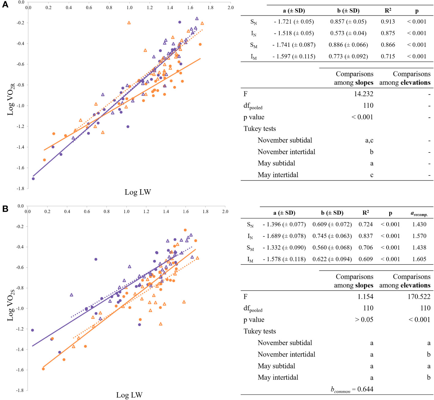
Figure 2 Regression lines for the allometric relationships of the form Y = a · Xb. (A) log- transformed routine oxygen consumption vs. log-transformed weight; (B) log-transformed standard oxygen consumption vs. log-transformed weight. On the top right of each figure, the allometric relationship is shown according to the expression: Y = a · LWb, where LW is live weight. In case of a common b-value, the recomputed a-values are also shown. On the bottom right, ANCOVA and post hoc tests. Shared letters (a, b or c) indicate no significant differences (p < 0.05). Purple and orange symbols distinguish tide levels (subtidal, intertidal), circles and triangles seasons (November, May). SN: purple circles; IN: orange circles; SM: purple triangles; IM: orange triangles.
Replacing the dummy variables, the following regression models arose for subtidal (0) and intertidal (1) mussels taking together the values for November and May:
The regression analysis of the model obtained the highest statistical significance (R2 = 0.829, F = 186.426 and p < 0.001).
3.1.2 Standard oxygen consumption (VO2S)
Data on standard oxygen consumption for each experimental group plotted as a function of their respective live weight can be found in Figure 2B. On the top right of Figure 2B, the resulting equations of such regressions are shown. For VO2S, no significant differences were found between slopes, therefore a common mass exponent (bc = 0.644) was computed. However, mass-specific standard oxygen consumption was significantly lower in intertidal mussels and, therefore, ANCOVA showed significant differences in intercepts between tide levels (Figure 2B).
3.1.3 Shell dimensions
Width vs. length. The individual shell widths for each mussel group have been plotted in Figure 3A as a function of their respective shell lengths. The resulting equations are shown on the top right of Figure 3A. No significant differences were found among slopes and a common allometric exponent (bc) of 0.393 was obtained (Figure 3A, bottom right). Intercepts were significantly higher in intertidal mussels, regardless of the season (Figure 3A, bottom right).
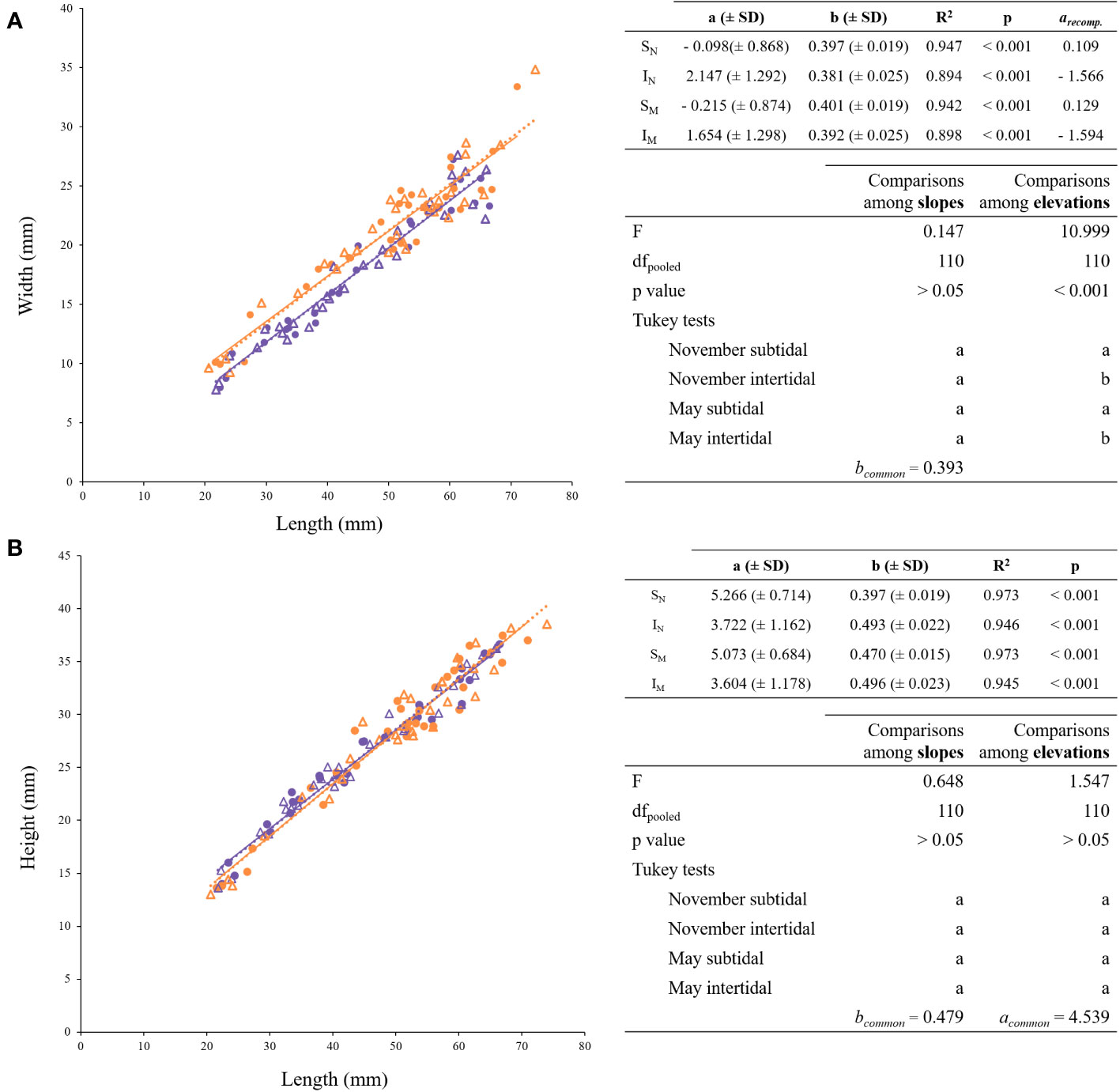
Figure 3 Regression lines for the allometric relationships of the form Y = bX - a (A) Shell width (mm) vs. Shell length (mm); (B) Shell height (mm) vs. Shell length (mm). On the top right of each figure, the allometric relationship for the shell dimension against individual length is shown. In case of a common b-value, the recomputed a-values are also shown (arecomp.). On the bottom right, ANCOVA and post hoc tests. Shared letters (a, b or c) indicate no significant differences (p< 0.05). Purple and orange symbols distinguish tide levels (Subtidal, Intertidal), circles and triangles seasons (November, May). SN: purple circles; IN: orange circles; SM: purple triangles; IM: orange triangles.
Height vs. length. The individual shell heights for each mussel group have been plotted in Figure 3B as a function of the respective shell length. No significant differences were found between slopes or intercepts, giving rise to a common regression (R2 = 0.959; p < 0.001; F = 2687.46) with an allometric exponent (bc) of 0.479 (± 0.009) and a common intercept (ac) of 4.539 (± 0.457). The common regression exponent values are shown on the bottom right table of Figure 3B.
SDW vs. length. The individual shell dry weights for each mussel group have been plotted in Figure 4A as a function of their respective shell lengths. The resulting equations are shown on the top right of Figure 4A. No significant differences were found among slopes and a common allometric exponent (bc) of 2.531 was obtained (Figure 4A, bottom right). Intercepts were significantly higher in intertidal mussels, regardless of the season (Figure 4A, bottom right).
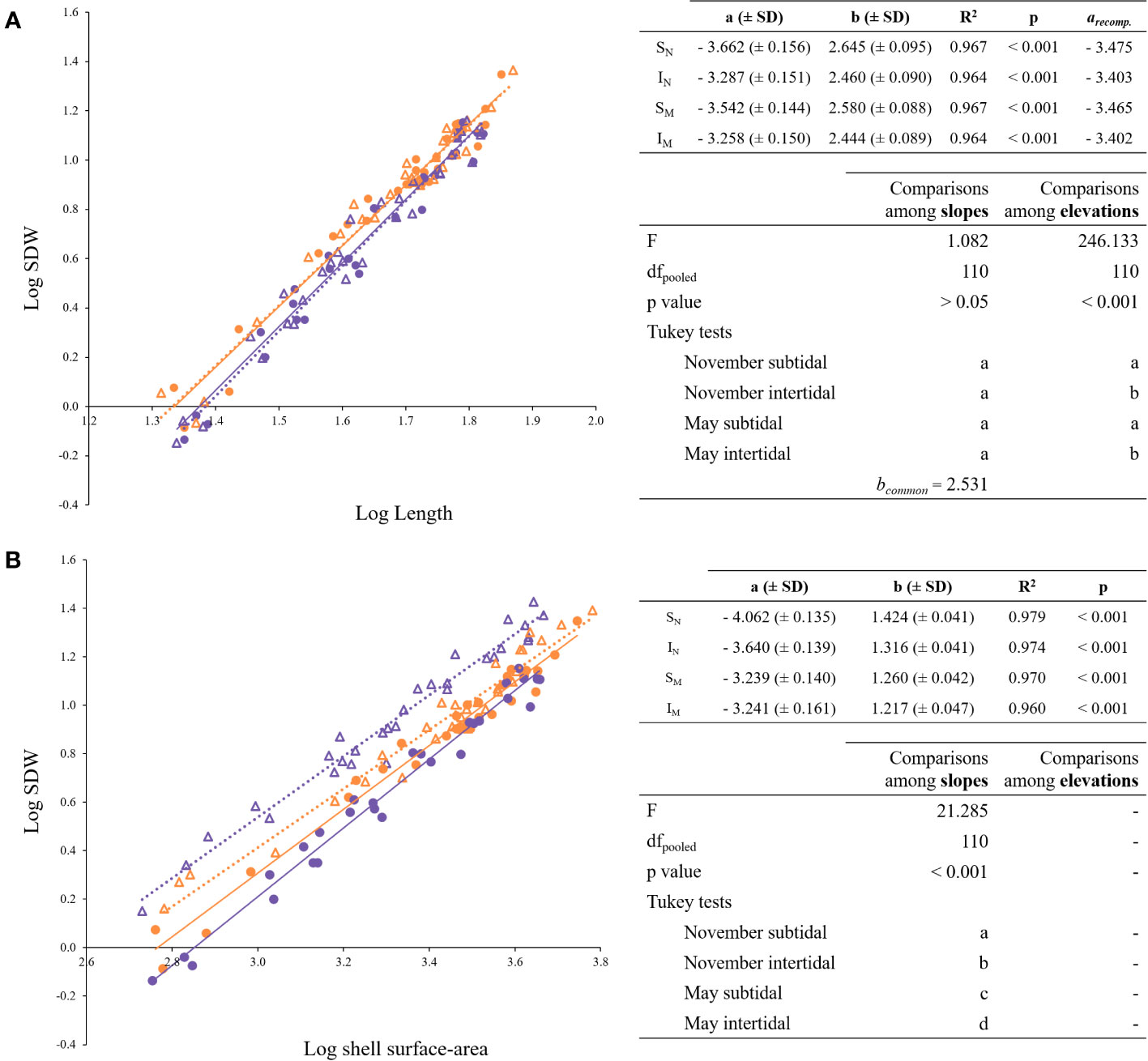
Figure 4 Regression lines for the allometric relationships of the form Y = a · Xb. (A) Log- transformed shell dry weight (SDW) vs. log-transformed shell length; (B) log-transformed shell dry weight (SDW) vs. log-transformed shell surface-area. On the top right of each figure, the allometric relationships are shown. On the bottom right, ANCOVA and post hoc tests. Shared letters (a, b or c) indicate no significant differences (p< 0.05). Purple and orange symbols distinguish tide levels (subtidal, intertidal), circles and triangles seasons (November, May). SN: purple circles; IN: orange circles; SM: purple triangles; IM: orange triangles.
SDW vs. surface-area. The individual shell dry weights for each mussel group have been plotted in Figure 4B as a function of their respective shell surface-areas. The b value corresponds to the effect that size exerts on the relationship between the two variables, whereas the a value represent what could be considered the density of the shell. The resulting equations are shown on the top right of Figure 4B. Each slope differed significantly from each other (Figure 4B, bottom right), being the differences between mussel groups smaller as the size increases. Also the intercepts indicate that the density of the shell is virtually the same in the intertidal mussels regardless of the season (for a common shell surface-area of 3.3: the a value for IM is 0.777 and for IN is 0.703). However, the shell density of subtidal individuals increases over a 30% in May compared to November (for a common shell surface-area of 3.3: the a value for SM is 0.916 and for SN is 0.636).
3.1.4 Condition index
Subtidal mussels from both seasons had around 30% higher CI (Figure 5), according to the Tukey test. The two-way ANOVA showed tide level as the only factor significantly affecting CI values (Figure 5, top right).
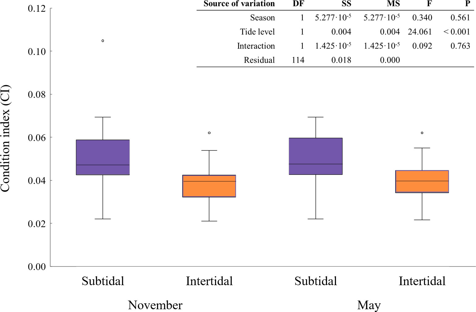
Figure 5 CI of subtidal and intertidal mussels for November and May. Shared letters indicate absence of statistical differences. On the top, the two-way factor ANOVA testing significant effects of season and tide level.
3.1.5 Gill surface-area
Figure 6 shows the relationship between gill-surface area and shell length in subtidal and intertidal mussels. The ANCOVA analysis showed no differences between slopes (t = 0.103, df = 1, 54; p > 0.05), with a bc value of 1.955. However, the intercept of intertidal mussels was higher compared to the subtidal mussels (t = 3.125, df = 1, 54; p < 0.001).
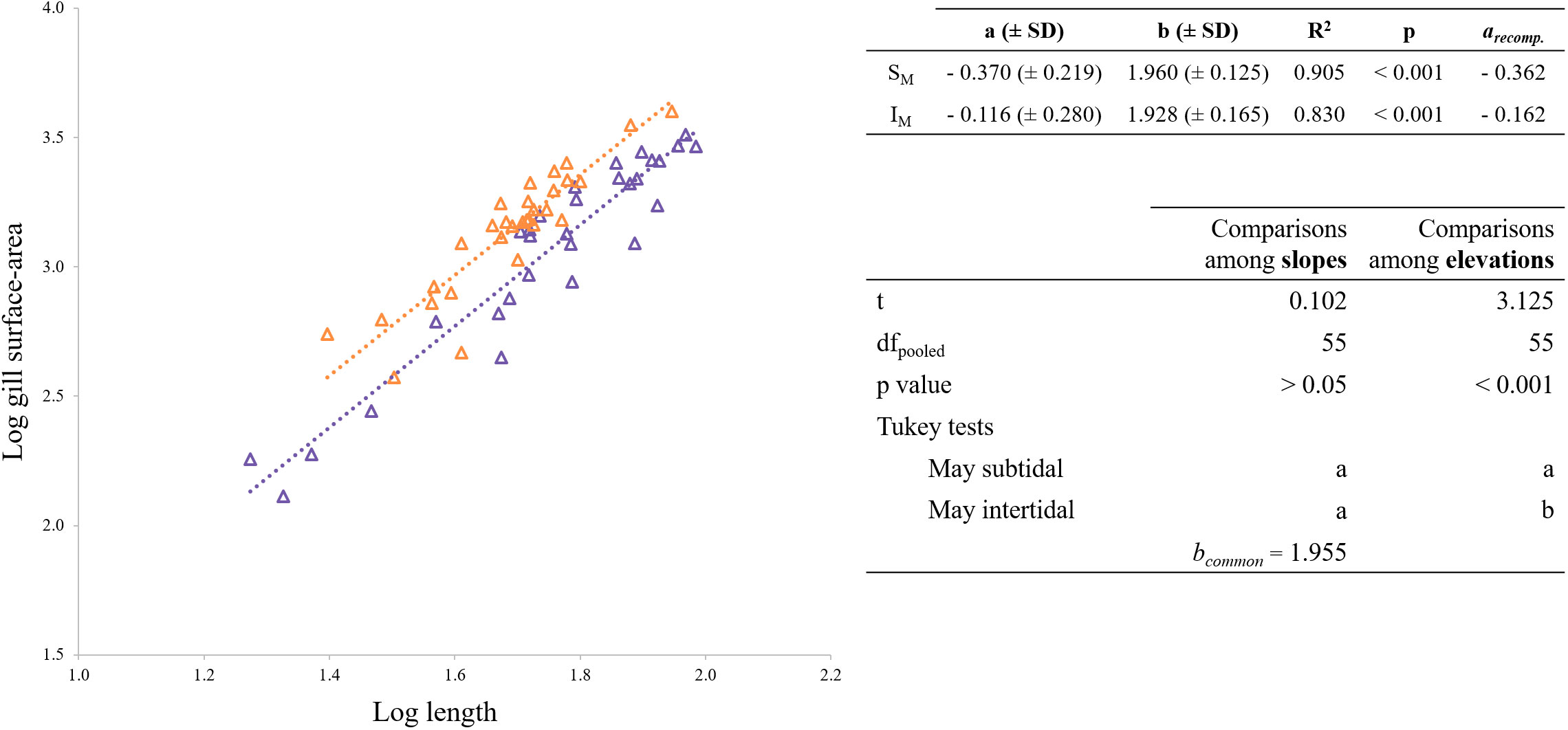
Figure 6 Regression lines for the allometric relationships of the form Y = a · Xb for gill-surface area against shell length. On the top right, the allometric relationship for the gill-surface area against individual length is shown. On the bottom right, ANCOVA and post hoc tests. Shared letters (a, b or c) indicate no significant differences (p< 0.05). Purple and orange symbols indicate values for subtidal and intertidal mussels, respectively.
3.2 Acclimation experiment
3.2.1 Routine oxygen consumption (VO2R)
Routine oxygen consumptions for each mussel group are plotted as a function of their respective live weight in Figure 7A and the resulting equations are summarized on the bottom right of the figure. The slopes of routine oxygen consumption and live weight differed from each other: intertidal mussels had lower allometric exponents, regardless of whether mussels were acclimated or not to laboratory conditions. Multiple regression analysis showed that live weight and tide explained 82% of the variation in routine oxygen consumption. The resulting general equation was the following (mean value ± SD):
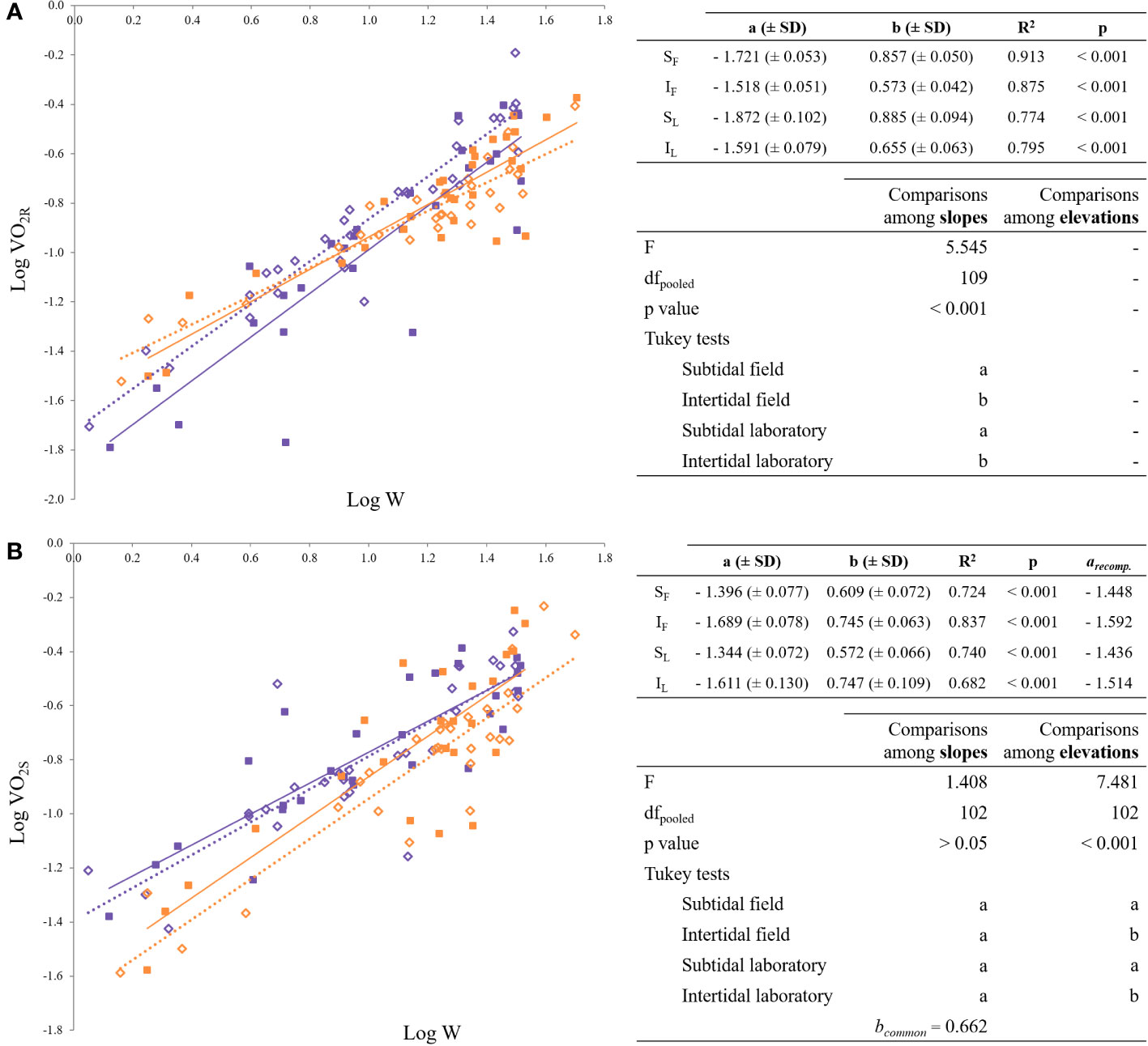
Figure 7 Regression lines for the allometric relationships of the form Y = a · Xb. (A) log- transformed routine oxygen consumption vs. log-transformed weight; (B) log-transformed standard oxygen consumption vs. log-transformed weight. Purple and orange rectangles distinguish tide levels (subtidal, intertidal); squares and diamonds distinguish acclimation time (field, lab). SF: purple diamonds; IF: orange diamonds; SL: purple squares; IL: orange squares.
Replacing the dummy variables, the following regression models arose for subtidal (0) and intertidal (1) mussels:
The regression analysis of the model obtained the highest statistical significance (R2 = 0.820, F = 171.944 and p < 0.001).
3.2.2 Standard oxygen consumption (VO2S)
The standard oxygen consumption data for each experimental group plotted as a function of their respective live weight can be found in Figure 7B. On the top right of Figure 7B, the resulting equations of such regressions are shown. For VO2S, the regression slopes were not significantly different (bc = 0.662), but the intercepts differed between the tide levels, with lower values for intertidal mussels (Figure 7B - bottom right).
4 Discussion
The broad intraspecific variability of the allometric mass-exponents of metabolic rate is a biological phenomenon not yet fully understood (e.g. Glazier, 2018; Hatton et al., 2019; Escala, 2022; White et al., 2022). The present experiment was designed to specifically analyze the range of variation of metabolic rate scaling values in a Mytilus galloprovincialis population covering a wide range of environmental conditions, including habitat differences (subtidal vs. intertidal) seasonal differences (May vs. November) and activity levels (standard vs. routine). The results reveal that the scaling values of the metabolic rate in mussels vary significantly from 0.56 to 0.88, with complex interactions of ecological and physiological factors.
The determination of individual values of standard and routine metabolic rates, a distinction hardly addressed for bivalve mollusks, has allowed us to confirm that the level of metabolic activity influences the value of the allometric exponent. That the activity development promotes higher b values has been suggested in the MLB hypothesis (Glazier, 2005; Glazier, 2008; Glazier, 2009; Glazier, 2010, Glazier, 2014) and reported in lobsters (Jensen et al., 2013) and chitons (Carey et al., 2013). When the activity level increases, the metabolic rate will become increasingly dominated by the energy demand of the tissues participating in the activity. For sessile organisms such as mussels, the activity refers primarily to the metabolic activity carried out by the organs participating in the food acquisition, digestion, assimilation and storage (Parry, 1983) as well as growth, development or reproduction (Glazier, 2005).
Interestingly, however, the effect of the level of activity recorded in this study differs significantly between subtidal and intertidal mussels. In subtidal mussels, the shift from standard to routine state promotes a significant increase of the scaling exponent from 0.64 to values of around 0.87, whereas changes in activity level did not exert significant changes in the metabolic scaling exponents of intertidal mussels. In contrast to our findings, Arranz et al. (2016) found no significant differences between size-scaling exponents of standard and routine metabolic rates in M. galloprovincialis, recording a common scaling exponent of 0.715 for both subtidal and intertidal specimens. It is noteworthy that the value reported by Arranz et al. (2016) falls in the middle of the range established in the present study for standard metabolic rate (bcommon = 0.644) and for routine metabolic rate of subtidal mussels (b = 0.875). Although there is a methodological difference in the oxygen consumption measurement between these two studies (group measurements in Arranz et al. (2016), vs. individual measurements here), the divergence of results suggests that the impact that the habitat exerts can considerably differ between sites. In fact, tidal level effects were reported by Marsden et al. (2012) when metabolic scaling exponents of different gastropod species were compared, suggesting that the effects imposed by habitat might be more general, affecting more species than M. galloprovincialis. Adaptation to the intertidal habitat involves the development of physiological mechanisms to overcome the daily cyclic periods of air exposure that promote desiccation, thermal stress and severe restrictions in food and oxygen supply. Intertidal mussels differ from subtidal mussels in their ability to survive hypoxia (Tagliarolo et al., 2012), desiccation (Babarro and De Zwaan, 2008) and thermal stress (Williams and Somero, 1996). Cross-transplantation experiments have shown that despite the considerable plasticity of physiological processes, metabolic differences between mussels of different habitats persist even after long periods of transplantation (Freites et al., 2002; Connor and Gracey, 2012; Gracey and Connor, 2016; Toone et al., 2023). This suggests the existence of fixed genetic differences between mussels of both origins. The possible existence of a selection process for the genotypes best suited to survive in the intertidal has, in fact, been raised in limpets by Clark et al. (2018), who showed that intertidal individuals expressed a distinctive and persistent genetic profile even after 9 months of transplantation. These set of genuine differences between subtidal and intertidal animals is coherent with the differences found herein that allow us to stablish a cause-effect relationship between habitats and scaling exponents.
In the present set of experiments, we have found significant differences between subtidal and intertidal mussels in relevant physiological and metabolic parameters that may contribute to the differential scaling of metabolic rates:
1. The level of standard metabolic rate depends on the origin of the mussels. Intertidal specimens consume approximately 26% less oxygen than subtidal mussels, regardless of the season or the acclimation. Furthermore, although intertidal mussels increased their standard oxygen consumption during acclimation to continuous immersion in the laboratory, habitat-linked differences persisted even after two months. Similar differences in Arranz et al. (2016) were attributed to an alleged higher gametogenic activity of subtidal mussels. This factor does not appear to contribute to the inter-habitat differences recorded here in metabolic rate, since in our study the differences were also reported in November, a season characterized by a resting gonadal phase in this mussel population (Azpeitia et al., 2017). Alternatively, lower standard metabolic rates in intertidal mussels could be related to daily oxygen deprivation during low tide. Although the anaerobic contribution cannot be overlooked (Gleason et al., 2017), hypometabolism is the usual strategy for coping with hypoxia in intertidal mollusks (Leeuwis and Gamperl, 2022), since the ATP amount supplied by anaerobic metabolism is rather small (Sokolova and Pörtner, 2001) and the “debt” accrued during low tide must be “paid” at high tide (Bayne, 1976).
2. The condition index recorded for mussels of different origins indicates that intertidal specimens have approximately 23% less flesh content than subtidal mussels. The values and differences recorded are consistent with previous studies (Arranz et al., 2016; Clark et al., 2018) and probably reflects habitat-linked growth-rate differences: (i) longer feeding periods of subtidal mussels, (ii) the use that intertidal mussels often do of energy storage to make up for food-shortage (Freites et al., 2002) and even (iii) a greater investment in shell (the present study –see below– and Beadman et al., 2003).
3. The energy investment of subtidal and intertidal mussels is allocated differently towards the different corporal fractions. The present experiment has shown that intertidal mussels have a larger gill-surface area for a given shell-length compared to their subtidal counterparts. Computation of the gill-surface area per flesh dry weight (mm2/mg dry flesh) shows that intertidal mussels have a 22% greater gill-surface area per FDW than subtidal mussels in November. In May, that difference increases up to a 29%. Thus, intertidal mussels selectively invest more in the production of the main organ involved in food acquisition, a worthy investment when faster growth is pursued (Pérez-Cebrecos et al., 2022). Despite habitat-linked differences, the gill-surface area increases proportionally to shell length in both cases with a scaling exponent of 1.955, which is very similar to that measured by Jones et al. (1992) for M. edulis (~ 2.06). Besides the gill, intertidal mussels also seem to invest specifically more in the shell-tissue, since the shell was systematically heavier notwithstanding the season when compared to subtidal mussels. Calculations from equations relating SDW with shell-length for subtidal and intertidal mussels show that for a common shell length of 40 mm, shell weight is 15 to 18% higher in intertidal mussels compared to subtidal individuals.
4. The shape and density of the shells differ between habitats. Intertidal mussels had an almost 7% greater gap (i.e. width) within the shells compared to subtidal mussels, which exhibited flatter shells. These proportions did not change as the mussels grew larger or across seasons, suggesting that the shell phenotype is beneficial for small and large mussels, and at any time of the year. In mollusks, shell dimensions are affected by environmental conditions (Clark et al., 2020). Babarro and Carrington (2013) reported lower and wider shells for exposed sites as a mechanism against wave dislodgement. Steffani and Branch (2003) also found lower shells at the exposed site, but this time narrower. In the present study, mussels were sampled from the same sheltered area of the rocky shore, and yet the gap within the shells differs greatly. However, shell height (i.e. narrower or wider) did not vary between tide-levels, which was also reported for sheltered sites in Babarro et al. (2020). A greater gap within the shells could contribute to mitigate desiccation and heat stress in intertidal mussels as described for limpets (Harley et al., 2009; Nuñez et al., 2018), and even to avoid hypoxia. A larger gap enables the enlargement of the air-pocket reserve during low tide, a typical strategy for having a source of oxygen. In limpets, for instance, a taller-shell ecotype has been described as a better way to survive hypoxia (Weihe and Abele, 2008).
The shell density also varies depending on the habitat. A change in the mean shell density can be explained either as a variation in the shell composition and/or a change in the shell thickness. The shell density variation of 30% in subtidal mussels might reflect a change in those two factors, indeed. On the one hand, November 2021 was especially rainy, with massive precipitations (Euskalmet (Agencia Vasca de Metereología), 2021) that predictably lowered the salinity of the estuary. Low salinity leads to low pH, making the layers of calcite and aragonite increase and decrease, respectively (Fitzer et al., 2015), implying a decrease in shell density. On the other hand, shell-thickening is a protective strategy: a higher shell density here recorded for intertidal mussels in May suggest that intertidal individuals invest more energy in protective tissues, since a thicker shell not only allows for increased mechanical protection, but it has also been reported to avoid heat stress (Harley et al., 2009) and desiccation (Staikou, 1999). The advantages that a denser and more convex shell confers to intertidal mussels seem to justify the greater investment in shell tissue described above.
If a primary outcome is to be gathered from the discussion above is that environmental conditions imposed by the habitat (subtidal versus intertidal) significantly affect phenotypic traits that can affect the size-scaling of metabolic rate such as i) the level of metabolic activity, ii) the growth rates and iii) the pattern of energy investment in the different body fractions, modifying not only the relative proportions of certain tissues, but even the morphology, shape and thickness of the organisms. These physiologic and anatomic factors provide a frame to understand the differences in the metabolic scaling that we have recorded in this population between intertidal and subtidal specimens. Intertidal animals showed manifestly lower scaling exponents and metabolic levels than subtidal mussels (closer to 2/3), a response that remained unchanged for at least two months after the environmental cue was removed. Compared to subtidal mussels, intertidal mussels have a lower metabolic activity and higher mass-proportion of tissues growing in a two-dimensional matrix: the gill and the shell. Thus, the scaling of routine oxygen consumption is mainly limited by fluxes of resources across surfaces imposing a scaling exponent closer to 2/3. A more exhaustive analysis of the allometric tendencies of intertidal mussels reinforces that notion. Although not statistically significant, a tendency to increase the b-exponent towards values closer to 1 in May could stem from the increasing energetic demands imposed by gonadal production, which promotes the thickening of the mantle (volume related resource requirements). In fact, this tendency of b-shifting in intertidal mussels resembles the findings of Iglesias and Navarro (1991) in Cerastoderma edule, in which a multiple regression analysis relating routine oxygen consumption with body weight and reproductive condition showed that b value shifts from 0.646 in the periods of sexual inactivity to 0.746 during seasons of reproductive activity. In contrast, in subtidal mussels the significant increase in the scaling value of metabolic rate in the transition from standard to routine states arises from their relatively (i) higher growth rates and metabolic levels and (ii) lower proportions of surface-related resource requirements due to the relatively lower investment in two-dimensional tissues such as shell and gills.
Data availability statement
The datasets presented in this study can be found in online repositories. The names of the repository/repositories and accession number(s) can be found below: Marine Data Archive repository: https://rb.gy/s9lf4.
Ethics statement
The manuscript presents research on animals that do not require ethical approval for their study.
Author contributions
MP-C: Conceptualization, Data curation, Investigation, Methodology, Writing – original draft. XB: Data curation, Investigation, Methodology, Writing – original draft. UI: Conceptualization, Formal Analysis, Funding acquisition, Project administration, Supervision, Validation, Writing – review & editing. II: Conceptualization, Formal Analysis, Funding acquisition, Project administration, Supervision, Validation, Writing – review & editing.
Funding
The author(s) declare financial support was received for the research, authorship, and/or publication of this article. This work was supported by the Basque Government through Consolidated Research Groups fellowship (CBET group, IT810-b) and through the predoctoral fellowship of MP-C.
Conflict of interest
The authors declare that the research was conducted in the absence of any commercial or financial relationships that could be construed as a potential conflict of interest.
Publisher’s note
All claims expressed in this article are solely those of the authors and do not necessarily represent those of their affiliated organizations, or those of the publisher, the editors and the reviewers. Any product that may be evaluated in this article, or claim that may be made by its manufacturer, is not guaranteed or endorsed by the publisher.
References
Abràmoff M. D., Magalhães P. J., Ram S. J. (2004). Image processing with ImageJ. Biophotonics. Int. 11 (7), 36–42. doi: 10.1038/nmeth.2089
Agutter P. S., Wheatley D. N. (2004). Metabolic scaling: consensus or controversy? Theor. Biol. Med. Model. 1, 1–11. doi: 10.1186/1742-4682-1-13
Alunno-Bruscia M., Bourget E., Fréchette M. (2001). Shell allometry and length-mass-density relationship for Mytilus edulis in an experimental food-regulated situation. Mar. Ecol. Prog. Ser. 219, 177–188. doi: 10.3354/meps219177
Anestis A., Pörtner H. O., Karagiannis D., Angelidis P., Staikou A., Michaelidis B. (2010). Response of Mytilus galloprovincialis (L.) to increasing seawater temperature and to marteliosis: metabolic and physiological parameters. Comp. Biochem. Physiol. Part A. Mol. Integr. Physiol. 156 (1), 57–66. doi: 10.1016/j.cbpa.2009.12.018
Arranz K., Labarta U., Fernández-Reiriz M. J., Navarro E. (2016). Allometric size- scaling of biometric growth parameters and metabolic and excretion rates. A comparative study of intertidal and subtidal populations of mussels (Mytilus galloprovincialis). Hydrobiologia 772, 261–275. doi: 10.1007/s10750-016-2672-3
Azpeitia K., Ortiz-Zarragoitia M., Revilla M., Mendiola D. (2017). Variability of the reproductive cycle in estuarine and coastal populations of the mussel Mytilus galloprovincialis Lmk. from the bay of Biscay (Basque Country). Int. Aquat. Res. 9 (4), 329–350. doi: 10.1007/s40071-017-0180-3
Babarro J. M., Carrington E. (2011). Byssus secretion of Mytilus galloprovincialis: effect of site at macro-and micro-geographical scales within ría de Vigo (NW Spain). Mar. Ecol. Prog. Ser. 435, 125–140. doi: 10.3354/meps09200
Babarro J. M., Carrington E. (2013). Attachment strength of the mussel Mytilus galloprovincialis: effect of habitat and body size. J. Exp. Mar. Biol. Ecol. 443, 188–196. doi: 10.1016/j.jembe.2013.02.035
Babarro J. M. F., De Zwaan A. (2008). Anaerobic survival potential of four bivalves from different habitats. A comparative survey. Comp. Biochem. Physiol. Part A. Mol. Integr. Physiol. 151 (1), 108–113. doi: 10.1016/j.cbpa.2008.06.006
Babarro J. M., Filgueira R., Padín X. A., Longa Portabales M. A. (2020). A novel index of the performance of Mytilus galloprovincialis to improve commercial exploitation in aquaculture. Front. Mar. Sci. 7. doi: 10.3389/fmars.2020.00719
Bayne B. L. (1976). Marine mussels: their ecology and physiology (Plymouth, UK: Cambridge University Press).
Bayne B. L., Hawkins A. J. S., Navarro E. (1988). Feeding and digestion in suspension-feeding bivalve molluscs: the relevance of physiological compensations. Am. Zool. 28 (1), 147–159. doi: 10.1093/icb/28.1.147
Bayne B. L., Newell R. C. (1983). “Physiological energetics of marine molluscs,” in The Mollusca (Plymouth, UK: Academic Press), 407–515.
Beadman H., Caldow R., Kaiser M., Willows R. (2003). How to toughen up your mussels: using mussel shell morphological plasticity to reduce predation losses. Mar. Biol. 142, 487–494. doi: 10.1007/s00227-002-0977-4
Bilbao J., Muñiz O., Rodríguez J. G., Revilla M., Laza-Martínez A., Seoane S. (2021). Assessment of a sheltered euhaline area of the southeastern Bay of Biscay to sustain bivalve production in terms of phytoplankton community composition. Oceanologia 63 (1), 12–26. doi: 10.1016/j.oceano.2020.08.007
Bokma F. (2004). Evidence against universal metabolic allometry. Funct. Ecol. 18 (2), 184–187. doi: 10.2307/3599357
Brown J. H., Gillooly J. F., Allen A. P., Savage V. M., West G. B. (2004). Toward a metabolic theory of ecology. Ecol 85 (7), 1771–1789. doi: 10.1890/03-9000
Burnett N. P., Belk A. (2018). Compressive strength of Mytilus californianus shell is time-dependent and can influence the potential foraging strategies of predators. Mar. Biol. 165, 1–9. doi: 10.1007/s00227-018-3298-y
Carey N., Sigwart J. D., Richards J. G. (2013). Economies of scaling: more evidence that allometry of metabolism is linked to activity, metabolic rate and habitat. J. Exp. Mar. Biol. Ecol. 439, 7–14. doi: 10.1016/j.jembe.2012.10.013
Clark M. S., Peck L. S., Arivalagan J., Backeljau T., Berland S., Cardoso J. C., et al. (2020). Deciphering mollusc shell production: the roles of genetic mechanisms through to ecology, aquaculture and biomimetics. Biol. Rev. 95 (6), 1812–1837. doi: 10.1111/brv.12640
Clark M. S., Thorne M. A., King M., Hipperson H., Hoffman J. I., Peck L. S. (2018). Life in the intertidal: cellular responses, methylation and epigenetics. Funct. Ecol. 32 (8), 1982–1994. doi: 10.1111/1365-2435.13077
Connor K. M., Gracey A. Y. (2012). High-resolution analysis of metabolic cycles in the intertidal mussel Mytilus californianus. Am. J. Physiol. Regul. Integr. Comp. Physiol. 302 (1), R103–R111. doi: 10.1152/ajpregu.00453.2011
Cordero-Rivera A., Ondina P., Outeiro A., Amaro R., San Miguel E. (2022). Allometry in the freshwater Pearl mussel (Margaritifera margaritifera L.): mussels tend to grow flatter at higher water speed. Malacologia 64 (2), 257–267. doi: 10.4002/040.064.0208
da Silva J. K. L., Garcia G. J., Barbosa L. A. (2006). Allometric scaling laws of metabolism. Phys. Life Rev. 3 (4), 229–261. doi: 10.1016/j.plrev.2006.08.001
Davenport J., Chen X. (1987). A comparison of methods for the assessment of condition in the mussel (Mytilus edulis l.). J. Molluscan. Stud. 53 (3), 293–297. doi: 10.1093/MOLLUS/53.3.293
Escala A. (2022). Universal relation for life-span energy consumption in living organisms: insights for the origin of aging. Sci. Rep. 12, 2407. doi: 10.1038/s41598-022-06390-6
Euskalmet (Agencia Vasca de Metereología). (2021). Data from: informe metereológico, noviembre 2021. departamento de seguridad del gobierno vasco. Available at: https://shorturl.at/cds59
Fitzer S. C., Zhu W., Tanner K. E., Phoenix V. R., Kamenos N. A., Cusack M. (2015). Ocean acidification alters the material properties of Mytilus edulis shells. J. R. Soc Interface 12 (103), 20141227. doi: 10.1098/rsif.2014.1227
Franz D. R. (1993). Allometry of shell and body weight in relation to shore level in the intertidal bivalve Geukensia demissa (Bivalvia: Mytilidae). J. Exp. Mar. Biol. Ecol. 174 (2), 193–207. doi: 10.1016/0022-0981(93)90017-I
Freites L., Labarta U., Fernández-Reiriz M. J. (2002). Evolution of fatty acid profiles of subtidal and rocky shore mussel seed (Mytilus galloprovincialis, Lmk.). Influence of environmental parameters. J. Exp. Mar. Biol. Ecol. 268 (2), 185–204. doi: 10.1016/S0022-0981(01)00377-X
Glazier D. S. (2005). Beyond the ‘3/4-power law’: variation in the intra-and interspecific scaling of metabolic rate in animals. Biol. Rev. 80 (4), 611–662. doi: 10.1017/S1464793105006834
Glazier D. S. (2008). Effects of metabolic level on the body size scaling of metabolic rate in birds and mammals. Proc. R. Soc B: Biol. Sci. 275 (1641), 1405–1410. doi: 10.1098/rspb.2008.0118
Glazier D. S. (2009). Activity affects intraspecific body-size scaling of metabolic rate in ectothermic animals. J. Comp. Physiol. B: Biochem. Syst. Environ. Physiol. 179, 821–828. doi: 10.1007/s00360-009-0363-3
Glazier D. S. (2010). A unifying explanation for diverse metabolic scaling in animals and plants. Biol. Rev. 85 (1), 111–138. doi: 10.1111/j.1469-185X.2009.00095.x
Glazier D. S. (2014). Metabolic scaling in complex living systems. Systems 2 (4), 451–540. doi: 10.3390/systems2040451
Glazier D. S. (2015). Is metabolic rate a universal ‘pacemaker’ for biological processes? Biol. Rev. 90 (2), 377–407. doi: 10.1111/brv.12115
Glazier D. S. (2018). Rediscovering and reviving old observations and explanations of metabolic scaling in living systems. Systems 6 (1), 4. doi: 10.3390/systems6010004
Glazier D. S. (2022a). How metabolic rate relates to cell size. Biol 11 (8), 1106. doi: 10.3390/biology11081106
Glazier D. S. (2022b). Variable metabolic scaling breaks the law: from ‘Newtonian’ to ‘Darwinian’ approaches. Proc. R. Soc B: Biol. Sci. 289 (1985), 20221605. doi: 10.1098/rspb.2022.1605
Gleason L. U., Miller L. P., Winnikoff J. R., Somero G. N., Yancey P. H., Bratz D., et al. (2017). Thermal history and gape of individual Mytilus californianus correlate with oxidative damage and thermoprotective osmolytes. J. Exp. Biol. 220 (22), 4292–4304. doi: 10.1242/jeb.168450
Gracey A. Y., Connor K. (2016). Transcriptional and metabolomic characterization of spontaneous metabolic cycles in Mytilus californianus under subtidal conditions. Mar. Genom. 30, 35–41. doi: 10.1016/j.margen.2016.07.004
Harley C. D., Denny M. W., Mach K. J., Miller L. P. (2009). Thermal stress and morphological adaptations in limpets. Funct. Ecol. 23, 292–301. doi: 10.1111/j.1365-2435.2008.01496.x
Hatton I. A., Dobson A. P., Storch D., Galbraith E. D., Loreau M. (2019). Linking scaling laws across eukaryotes. PNaS 116 (43), 21616–21622. doi: 10.1073/pnas.1900492116
Hawkins A. J. S., Navarro E., Iglesias J. I. P. (1990). Comparative allometries of gut-passage time, gut content and metabolic faecal loss in Mytilus edulis and Cerastoderma edule. Mar. Biol. 105, 197–204. doi: 10.1007/BF01344287
Hemmingsen A. M. (1960). Energy metabolism as related to body size and respiratory surfaces, and its evolution. Rep. Steno. Mem. Hosp. Nord. Insulin. Lab. 9, 3–110.
Hirst A. G., Glazier D. S., Atkinson D. (2014). Body shape shifting during growth permits tests that distinguish between competing geometric theories of metabolic scaling. Ecol. Lett. 17 (10), 1274–1281. doi: 10.1111/ele.12334
Ibarrola I., Arranz K., Markaide P., Navarro E. (2022). Metabolic size scaling reflects growth performance effects on age-size relationships in mussels (Mytilus galloprovincialis). PloS One 17 (9), e0268053. doi: 10.1371/journal.pone.0268053
Iglesias J. I. P., Navarro E. (1991). Energetics of growth and reproduction in cockles (Cerastoderma edule): seasonal and age-dependent variations. Mar. Biol. 111, 359–368. doi: 10.1007/BF01319407
Jensen M. A., Fitzgibbon Q. P., Carter C. G., Adams L. R. (2013). Effect of body mass and activity on the metabolic rate and ammonia-n excretion of the spiny lobster Sagmariasus verreauxi during ontogeny. Comp. Biochem. Physiol. Part A. Mol. Integr. Physiol. 166 (1), 191–198. doi: 10.1016/j.cbpa.2013.06.003
Jones H. D., Richards O. G., Southern T. A. (1992). Gill dimensions, water pumping rate and body size in the mussel Mytilus edulis. J. Exp. Mar. Biol. Ecol. 155 (2), 213–237. doi: 10.1016/0022-0981(92)90064-H
Kleiber M. (1932). Body size and metabolism. Hilgardia 6 (11), 315–353. doi: 10.3733/hilg.v06n11p315
Kozlowski J., Konarzewski M., Gawelczyk A. T. (2003). Cell size as a link between noncoding DNA and metabolic rate scaling. PNAS 100 (24), 14080–14085. doi: 10.1073/pnas.2334605100
Kozlowski J., Konarzewski M., Gawelczyk A. T. (2020). Coevolution of body size and metabolic rate in vertebrates: a life-history perspective. Biol. Rev. 95 (5), 1393–1417. doi: 10.1111/brv.12615
Leeuwis R. H. J., Gamperl A. K. (2022). “Adaptations and plastic phenotypic responses of marine animals to the environmental challenges of the high intertidal zone,” in Oceanogr. Mar. Biol. Eds. Hawkins S. J., Allcock A. L., Bates A. E., Byrne M., Evans A. J., Firth L. B., Lemasson A. J., Lucas C., Marzinelli E. M., Mumby P. J., Russell B. D., Sharples J., Smith I. P., Swearer S. E., Todd P. A. (Boca Ratón, Florida, United States: CRC Press), 625–679. doi: 10.1201/9781003288602-13
Mandic M., Regan M. D. (2018). Can variation among hypoxic environments explain why different fish species use different hypoxic survival strategies? J. Exp. Biol. 221 (21), jeb161349. doi: 10.1242/jeb.161349
Marsden I. D., Shumway S. E., Padilla D. K. (2012). Does size matter? The effects of body size and declining oxygen tension on oxygen uptake in gastropods. J. Mar. Biol. Assoc. 92 (7), 1603–1617. doi: 10.1017/S0025315411001512
McArley T. J., Hickey A. J., Wallace L., Kunzmann A., Herbert N. A. (2019). Intertidal triplefin fishes have a lower critical oxygen tension (p crit), higher maximal aerobic capacity, and higher tissue glycogen stores than their subtidal counterparts. J. Comp. Physiol. B: Biochem. Syst. Environ. Physiol. 189 (3-4), 399–411. doi: 10.1007/s00360-019-01216-w
Muller-Landau H. C., Condit R. S., Chave J., Thomas S. C., Bohlman S. A., Bunyavejchewin S., et al. (2006). Testing metabolic ecology theory for allometric scaling of tree size, growth and mortality in tropical forests. Ecol. Lett. 9 (5), 575–588. doi: 10.1111/j.1461-0248.2006.00904.x
Nicastro K. R., Zardi G. I., McQuaid C. D., Stephens L., Radloff S., Blatch G. L. (2010). The role of gaping behaviour in habitat partitioning between coexisting intertidal mussels. BMC Ecol. 10, 1–11. doi: 10.1186/1472-6785-10-17
Nuñez J. D., Fernández Iriarte P., Ocampo E. H., Madrid E., Cledón M. (2018). Genetic and morpho-physiological differentiation in a limpet population across an intertidal gradient. Helgol. Mar. Res. 72, 1–10. doi: 10.1186/s10152-018-0519-1
O’Connor M. P., Kemp S. J., Agosta S. J., Hansen F., Sieg A. E., Wallace B. P., et al. (2007). Reconsidering the mechanistic basis of the metabolic theory of ecology. Oikos 116 (6), 1058–1072. doi: 10.1111/j.0030-1299.2007.15534.x
Parry G. D. (1983). The influence of the cost of growth on ectotherm metabolism. J. Theor. Biol. 101 (3), 453–477. doi: 10.1016/0022-5193(83)90150-9
Pérez-Cebrecos M., Prieto D., Blanco-Rayón E., Izagirre U., Ibarrola I. (2022). Differential tissue development compromising the growth rate and physiological performances of mussel. Mar. Environ. Res. 180, 105725. doi: 10.1016/j.marenvres.2022.105725
Prieto D., Tamayo D., Urrutxurtu I., Navarro E., Ibarrola I., Urrutia M. (2020). Nature more than nurture affects the growth rate of mussels. Sci. Rep. 10 (1), 1–13. doi: 10.1038/s41598-020-60312-y
Prieto D., Urrutxurtu I., Navarro E., Urrutia M., Ibarrola I. (2018). Mytilus galloprovincialis fast growing phenotypes under different restrictive feeding conditions: Fast feeders and energy savers. Mar. Environ. Res. 140, 114–125. doi: 10.1016/j.marenvres.2018.05.007
Reimer O., Tedengren M. (1996). Phenotypical improvement of morphological defences in the mussel Mytilus edulis induced by exposure to the predator Asterias rubens. Oikos 75 (3), 383–390. doi: 10.2307/3545878
Sarà G., Pusceddu A. (2008). Scope for growth of Mytilus galloprovincialis (Lmk. 1819) in oligotrophic coastal waters (southern Tyrrhenian sea, Italy). Mar. Biol. 156, 117–126. doi: 10.1007/s00227-008-1069-x
Savage V. M., Gillooly J. F., Woodruff W. H., West G. B., Allen A. P., Enquist B. J., et al. (2004). The predominance of quarter-power scaling in biology. Funct. Ecol. 18 (2), 257–282. doi: 10.1111/j.0269-8463.2004.00856.x
Sokolova I., Pörtner H. (2001). Temperature effects on key metabolic enzymes in Littorina saxatilis and L. obtusata from different latitudes and shore levels. Mar. Biol. 139, 113–126. doi: 10.1007/s002270100557
Sprung M. (1984). Physiological energetics of mussel larvae (Mytilus edulis). 111. Respiration. Mar. Ecol. Prog. Ser. 18, 171. doi: 10.3354/meps018171
Staikou A. E. (1999). Shell temperature, activity and resistance to desiccation in the polymorphic land snail Cepaea vindobonensis. J. Molluscan. Stud. 65 (2), 171–184. doi: 10.1093/mollus/65.2.171
Steffani C. N., Branch G. M. (2003). Growth rate, condition, and shell shape of Mytilus galloprovincialis: responses to wave exposure. Mar. Ecol. Prog. Ser. 246, 197–209. doi: 10.3354/meps246197
Suarez R. K., Darveau C. A., Childress J. J. (2004). Metabolic scaling: a many- splendoured thing. Comp. Biochem. Physiol. B Biochem. Mol. Biol. 139 (3), 531–541. doi: 10.1016/j.cbpc.2004.05.001
Tagliarolo M., Clavier J., Chauvaud L., Koken M., Grall J. (2012). Metabolism in blue mussel: intertidal and subtidal beds compared. Aquat. Biol. 17, 167–180. doi: 10.3354/ab00464
Tamayo D., Azpeitia K., Markaide P., Navarro E., Ibarrola I. (2016). Food regime modulates physiological processes underlying size differentiation in juvenile intertidal mussels Mytilus galloprovincialis. Mar. Biol. 163, 1–13. doi: 10.1007/s00227-016-2905-z
Tokeshi M., Ota N., Kawai T. (2000). A comparative study of morphometry in shell-bearing molluscs. J. Zool. 251 (1), 31–38. doi: 10.1111/j.1469-7998.2000.tb00590.x
Toone T. A., Hillman J. R., Benjamin E. D., Handley S., Jeffs A. (2023). Out of their depth: The successful use of cultured subtidal mussels for intertidal restoration. Conserv. Sci. Pract. 5 (4), e12914. doi: 10.1111/csp2.12914
Weihe E., Abele D. (2008). Differences in the physiological response of inter-and subtidal antarctic limpets Nacella concinna to aerial exposure. Aquat. Biol. 4 (2), 155–166. doi: 10.3354/ab00103
White C. R. (2011). Allometric estimation of metabolic rates in animals. Comp. Biochem. Physiol. Part A. Mol. Integr. Physiol. 158 (3), 346–357. doi: 10.1016/j.cbpa.2010.10.004
White C. R., Alton L. A., Bywater C. L., Lombardi E. J., Marshall D. J. (2022). Metabolic scaling is the product of life-history optimization. Evol. Ecol. 377 (6608), 834–839. doi: 10.1126/science.abm7649
White C. R., Phillips N. F., Seymour R. S. (2006). The scaling and temperature dependence of vertebrate metabolism. Biol. Lett. 2 (1), 125–127. doi: 10.1098/rsbl.2005.0378
Williams E. E., Somero G. N. (1996). Seasonal-, tidal-cycle- and microhabitat-related variation in membrane order of phospholipid vesicles from gills of the intertidal mussel mytilus californianus. J. Exp. Biol. 199 (7), 1587–1596. doi: 10.1242/jeb.199.7.1587
Winter J. E. (1978). A review on the knowledge of suspension-feeding in lamellibranchiate bivalves, with special reference to artificial aquaculture systems. Aquac 13 (1), 1–33. doi: 10.1016/0044-8486(78)90124-2
Keywords: Mytilus galloprovincialis, allometry, metabolic scaling, habitat, tide level, metabolic level boundaries hypothesis (MLB)
Citation: Pérez-Cebrecos M, Berrojalbiz X, Izagirre U and Ibarrola I (2023) Metabolic scaling variation as a constitutive adaptation to tide level in Mytilus galloprovincialis. Front. Mar. Sci. 10:1289443. doi: 10.3389/fmars.2023.1289443
Received: 05 September 2023; Accepted: 24 October 2023;
Published: 08 November 2023.
Edited by:
Valerio Matozzo, University of Padua, ItalyReviewed by:
Marco Munari, University of Padua, ItalyDouglas Stewart Glazier, Juniata College, United States
Camilla Bertolini, Ca’ Foscari University of Venice, Italy
Copyright © 2023 Pérez-Cebrecos, Berrojalbiz, Izagirre and Ibarrola. This is an open-access article distributed under the terms of the Creative Commons Attribution License (CC BY). The use, distribution or reproduction in other forums is permitted, provided the original author(s) and the copyright owner(s) are credited and that the original publication in this journal is cited, in accordance with accepted academic practice. No use, distribution or reproduction is permitted which does not comply with these terms.
*Correspondence: Maitane Pérez-Cebrecos, bWFpdGFuZS5wZXJlekBlaHUuZXVz