Groundwater nutrient loading into the northern Indian River lagoon: measurements and modeling

The Indian River Lagoon System (IRLS) has been impacted by the surrounding development, leading to excessive nutrient loads that have resulted in frequent and prolonged phytoplankton blooms in the northern reaches. Our study focused on estimating terrestrial groundwater discharge (TGD) and associated nutrient loads by combining field measurements and hydrogeologic modeling at four transects: Eau Gallie (EGT), River Walk (RWT), Banana River (BRT), and Mosquito Lagoon (MLT) across the IRLS. Multiple monitoring stations were installed to collect groundwater and surface water levels, salinity, and nutrient concentrations during 2014-2015. Samples were analyzed for dissolved inorganic nitrogen (DIN) and dissolved inorganic phosphorus (DIP). Numerical modeling was accomplished using SEAWAT to simulate TGD rates, whereas nutrient loads were calculated by multiplying simulated TGD by measured concentrations. TGD rates and nutrient loads were also estimated specifically for the “near-shore zone” along each transect. The effect of recharge from underlying Hawthorn Formation was also evaluated by incorporating estimated recharge rates into the models. Porewater and lagoon water samples showed that ammonium predominated over (NO₂+NO₃) and PO₄ at all sites, resulting in DIN/DIP ratio surpassing the Redfield ratio. Low nitrite/nitrate, coupled with elevated ammonium concentrations at RWT, BRT, and MLT, may be attributed to biogeochemical transformations catalyzed by mangroves and wetlands. Simulated TGD showed mild temporal but significant spatial variation, especially between EGT and RWT compared to BRT and MLT. The highest average TGD of 0.73 and 0.77 m³/d.m occurred at RWT and EGT, respectively, whereas the lowest rates were predicted at BRT and MLT. The highest estimated average DIN loads of 507 and 428 g/yr.m were received at EGT and RWT, respectively, whereas MLT and BRT exhibited lower loads. The DIP loads were remarkably lower than the DIN loads and were significantly different in space and time between sites. Elevated DIN combined with reduced DIP resulted in DIN/DIP exceeding the Redfield ratio, thereby encouraging the blooming of harmful algae. Although the majority of seepage occurs through the near-shore zone, small amounts are received along the entire transect at all sites. The Hawthorn Formation does not contribute significant recharge to the aquifer at the transect locations.

1 Introduction

Coastal waters receive groundwater discharge in two forms: a fresh constituent that originates from terrestrial recharge of shallow aquifers and moves seaward, and a saline constituent that originates from the sea, moves landward along the base of the coastal aquifer, and recirculates back to the sea at the upper portion of the aquifer (Moore and Church, 1996). Moore (1999) proposed the term “subterranean estuary” to characterize this particular coastal flow system. The fresh portion of groundwater discharge is known as meteoric or terrestrial groundwater discharge (TGD) and is driven by terrestrial groundwater hydraulic gradient, while the saline portion is termed recirculated groundwater discharge (RGD) and is governed by coastal processes such as wave action and tidal pumping (Moore, 2010; Taniguchi et al., 2019). Taniguchi et al. (2002) define the summation of the TGD and RGD as the total submarine groundwater discharge (SGD). The seaward movement of TGD under advective forces and the recirculation of RGD create a mixing action between the two components and form a miscible, finite brackish transition zone (BTZ). The groundwater density across the BTZ varies from freshwater density to seawater density, and thus, groundwater physics in coastal aquifers is density-dependent (Bear, 1979).

Although both fresh and saline SGD components play an essential role in biogeochemical cycles and water budgets in coastal zones (Knee and Paytan, 2011), it is recognized that TGD is the main conduit that delivers new terrestrial solutes and biolimiting nutrients like nitrogen and phosphorus generated by anthropogenic sources such as pesticides, domestic wastewater, and fertilizers to coastal waters (Pavlidou et al., 2014; Luijendijk et al., 2020; Szymczycha et al., 2020). RGD, as opposed to TGD, only contributes recycled nutrients washed out of the sediments (Wilson, 2005; Santos et al., 2009). Furthermore, in regions where surface runoff is restricted, TGD is usually the lone source of terrestrial nutrients and pollutants (Burnett et al., 2006). Ubiquitous environmental impacts of TGD-delivered nutrients on coastal waters have been reported, such as increased benthic productivity (Carruthers et al., 2005; Waska and Kim, 2010) and the occurrence of harmful algal blooms and fish die-off (Phlips et al., 2002; Hu et al., 2006; Howarth, 2008; Kwon et al., 2017; Montiel et al., 2019). TGD-related cascades of impacts have been noticed to occur in various coastal systems, including estuaries (Charette and Buesseler, 2004; Liu et al., 2018) and lagoons (Lee et al., 2009; Liefer et al., 2014). Thus, protection of the quality of coastal waters and ensuring the well-being of coastal communities require management practices that incorporate SGD and its derived nutrient loads in water management plans. However, compared to surficial point source discharges such as riverine inputs, quantifying SGD is challenging as it is a subsurface process, that is diffusive and highly variable in space and time. The difficulty in quantifying SGD has usually led to overpassing its nutrient fluxes in coastal nutrient budgets (Sawyer et al., 2016).

The last few decades have witnessed the advent of several approaches and techniques to quantify SGD including seepage meters studies (Belanger and Walker, 1990; Michael et al., 2003; Taniguchi et al., 2006), radon and radium isotopes such as ^{223,224,226,228}Ra and ^220,222Rn as geochemical tracers (Cable et al., 1996; Moore, 1996; Burnett et al., 2001; Chanyotha et al., 2014; Cabral et al., 2023), hydrogeological groundwater modeling (Oberdorfer, 2003; Al-Taliby et al., 2016; Russoniello et al., 2018; Evans et al., 2020; Al-Taliby and Pandit, 2023), thermal imaging using infrared sensors (Johnson et al., 2008; Wilson and Rocha, 2012), and geophysical methods like electrical resistivity (Swarzenski et al., 2006; Dimova et al., 2012). The majority of SGD flux measurement research employed Ra and Rn isotopes and seepage meters (Burnett et al., 2006; Santos et al., 2021). What makes Ra and Rn good tools for SGD flux mass balance-based estimation is that they are enriched in groundwater and diminished in seawater. However, even with their advantages, natural tracer mass balance models have limitations and drawbacks, including high cost and experienced staff requirements, being more appropriate for karstic and fractured aquifer systems (Burnett et al., 2006), and their lack of ability to differentiate between TGD and RGD and just revealing total SGD flux, which results in overestimated terrestrial nutrient fluxes (Santos et al., 2021). Other limitations of using geochemical tracers in the context of SGD studies are reported by Lino et al. (2023). Despite its advantage in yielding direct measurement of SGD, seepage meters have also been reported to be susceptible to several defects such as: i) their localized measurement that is limited to a small area of ~0.25 m² and thus, clusters of seepage meters are usually deployed to acquire representative measurement because SGD is known to be patchy and diffusive, ii) their measurement is only reliable when flux rate is higher than ~5 cm/d, iii) when flux rate is low, seepage meters may easily be affected by coastal currents and wave actions resulting in overestimated SGD fluxes, and iv) the collected sample is a mixture of TGD and SGD, which may prevent the differentiation between the two components to precisely estimate their nutrient loads separately (Belanger and Montgomery, 1992; Corbett and Cable, 2003; Michael et al., 2003; Burnett et al., 2006; Santos et al., 2021). Although both thermal infrared imagery and resistivity methods can discriminate between TGD and RGD, they are particularly applicable in limited regions such as karst coastal aquifers where the temperature and density contrast between SGD and the receiving coastal environments is profoundly considerable to be captured by satellites or conductivity probes (Johnson et al., 2008; Stieglitz et al., 2008; Tamborski et al., 2015). Also, SGD measurements conducted using these two geophysical techniques must usually be combined with other quantification techniques (Taniguchi et al., 2019), resulting in considerable costs.

Hydrogeologic modeling easily enables the incorporation of meteoric sources of groundwater and thus provides a good tool for tracking and quantifying TGD. Hydrogeologic modeling has been used in fewer research studies to quantify SGD (Kaleris et al., 2002; Langevin, 2003; Oberdorfer, 2003; Russoniello et al., 2018; Evans et al., 2020; Al-Taliby and Pandit, 2023). To properly account for density effects in coastal aquifers, some of the numerical modeling studies dedicated to SGD research have utilized variable-density models, albeit most of them (Kaleris et al., 2002; Langevin, 2003; Smith and Zawadzki, 2003; Evans et al., 2020) have concentrated on calculating the total SGD rate and not the fresh component (TGD), which is the main conduit that contributes new SGD-born terrestrial nutrients to coastal waters. The few numerical modeling investigations that quantified TGD (Pandit and El-Khazen, 1990; Unnikrishnan et al., 2021) relied on constant-density modeling techniques that neglect density gradients. Hydrogeologic modeling efforts mentioned above were entirely focused on predicting SGD rates, without estimating their associated nutrient loads.

This study was designed to combine field measurements and variable-density numerical models to quantify TGD fluxes and their associated macronutrients, i.e., dissolved inorganic nitrogen (DIN) and dissolved inorganic phosphorus (DIP) loads, into an estuarine system, known as the Indian River Lagoon system (IRLS). The IRLS spans a vast unconfined aquifer where the underlying confining layer is sometimes absent. As a result, it remains uncertain whether the confined aquifer beneath recharges the unconfined portion significantly in areas underneath the lagoon. This study had three specific objectives: 1) determine the TGD rates and the associated DIN and DIP loads carried into the lagoon at four transects across the northern reaches of the IRLS, 2) determine and contrast the seepage and loadings between the “near-shore zone” and the entire transect, and 3) investigate the effect of recharge from an aquitard, known as the Hawthorn Formation, below the unconfined aquifer. The purpose of conducting the study at four different transects is to determine whether there are heterogeneities in TGD rates and their driven nutrients between sites along the lagoon with similar hydrogeological conditions, but different land uses and coastal characteristics.

2 Study area

2.1 Site description

The estuarine system selected for conducting this study is the Indian River Lagoon system (IRLS), a coastal estuary in Florida, USA (Figure 1). This site spans approximately 250 km of the alluvial plains on the eastern Atlantic coast of Florida from Volusia County to Palm Beach County. Hydraulic connection of the IRLS to the Atlantic Ocean occurs through two natural inlets, those are the Ponce de Leon Inlet in Volusia County at the north end and the Jupiter Inlet in Palm Beach County at the south end. In between, additional connection to the ocean occurs through three engineered inlets, the Sebastian, the Fort Pierce, and the St. Lucie Inlets. Along the coast, the lagoon is protected from the ocean by the Barrier Island, a chain of coastal islands. The IRLS’s water body consists of three shallow micro tidal lagoons: the Indian River (IRL), the Banana River (BRL), and the Mosquito Lagoon (ML) as shown in Figure 1. Spanning ~220 km, the IRL is the longest lagoon of the system. The BRL is approximately 57 km long and is detached from the IRL by a thin land mass known as Merritt Island (Figure 1). A much smaller lagoon, the ML, lies just north of the IRL. The width of the various lagoons varies from 0.8–8.0 km and the depths of water vary from 1 to 5 m.

FIGURE 1

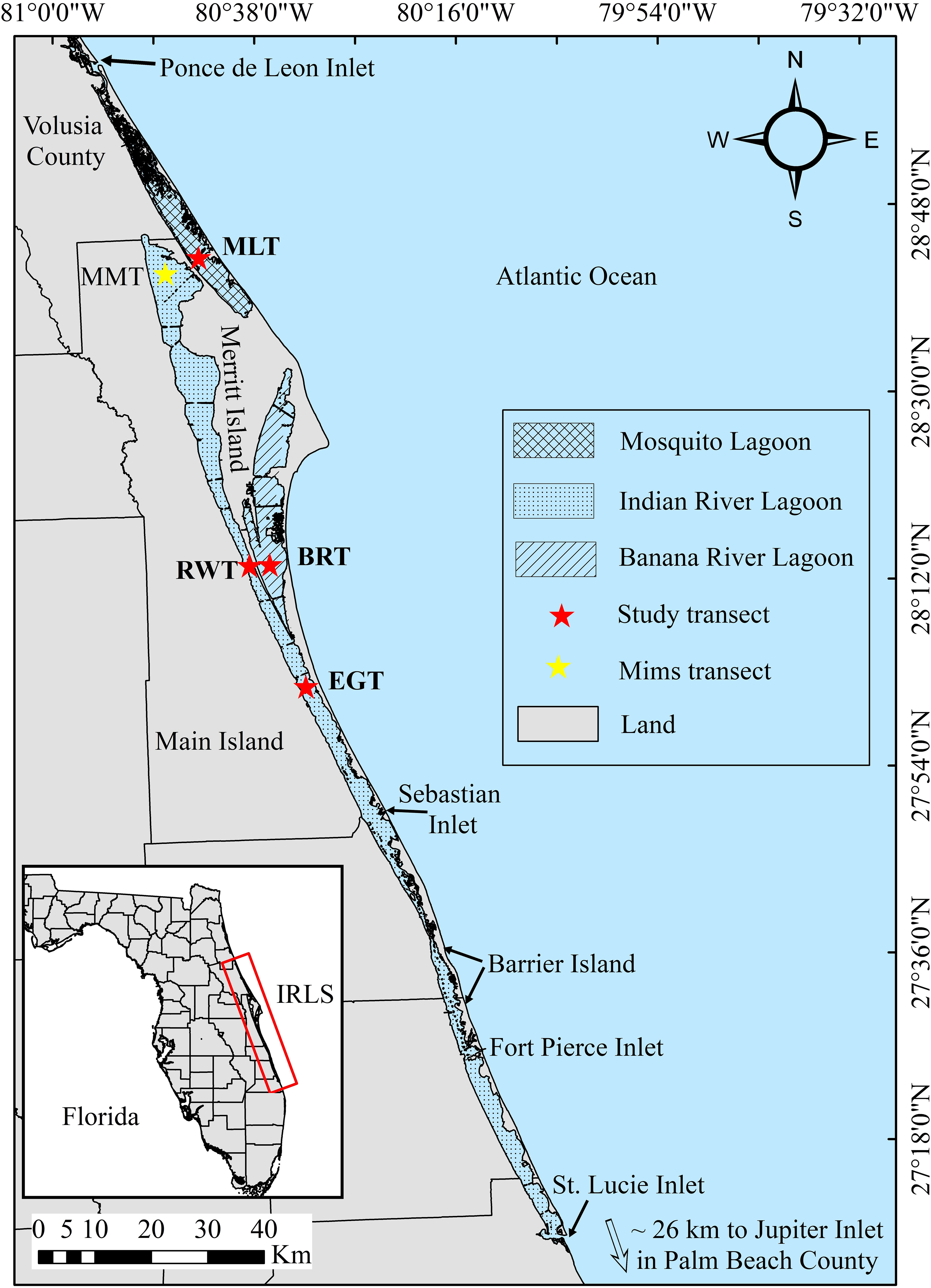
Figure 1 Indian River Lagoon system and locations of the study transects.

With thousands of species living in the IRLS watershed as their habitat, the system possesses its position as one of the most important biodiverse ecological sites in the U.S. (Gilmore et al., 1983). Most of the ecological importance of the estuarine system comes from the presence of seagrass that covers the bottom of the lagoonal system at many places (Dawes et al., 1995). The IRLS watershed has been changed by urban and agricultural development that increased extensively over the last few decades, resulting in the decline of the IRLS water quality due to the received pollutants, particularly nitrogen and phosphorus through multiple pathways in surface and ground waters (Sigua and Tweedale, 2003). The key issue is that this estuarine ecosystem is becoming more eutrophic as a result of excessive nutrient loading, especially in the northern reaches where significant phytoplankton blooms lasting more than a month have increased in frequency. Seagrass cover loss and huge masses of harmful algal blooms have been reported to occur in the IRLS more frequently (Phlips et al., 2004; Steward et al., 2005; St. Johns River Water Management District, 2012). Recent aerial imagery studies estimated that about 58% of seagrass extent vanished between the years 2011-2019 (Morris et al., 2022).

2.2 Site hydrogeology and hydrology

In terms of the hydrogeologic setting of the IRLS, the uppermost hydrostratigraphic unit below the study area is the surficial unconfined aquifer (SUA) which consists mainly of quaternary Holocene and Pleistocene age sand and sandy coquina deposits, characterized by low to moderate permeability and yields minor groundwater quantities (Miller, 1986). Below the SUA is the intermediate unit known as the Hawthorn Formation which consists mainly of low-permeability Miocene deposits of clay, marl, and dolomite. The depth from the sandy SUA layer down to the Hawthorn Formation ranges between (28.5 - 44 m) at the study site (Miller, 1986). The third main hydrostratigraphic formation in the area, which is confined by the Hawthorn Formation, is the artesian aquifer, known as the upper Floridan aquifer (UFA) (Miller, 1986; Scott, 1988). The UFA is a huge aquifer system that covers the entire state of Florida and parts of the neighboring states and is composed of Paleocene to early Miocene beds of limestone and dolomite. Yielding very large amounts of groundwater, the UFA is considered one of the principal groundwater resources in the U.S. (Bush and Johnston, 1988). It is generally assumed that the groundwater discharging into the IRLS is primarily from the SUA with negligible input from the UFA due to the presence of the Hawthorn Formation. However, the Hawthorn Formation is absent at some locations below the IRLS causing the UFA to be leaky or semiconfined at those locations (Berndt et al., 2014), thus, it is likely that there may be significant recharge from the UFA through the Hawthorn Formation in some areas below the IRLS.

Regarding the site hydrologic conditions, the area is dominated by a subtropical climatic setting which is hot (average temperature range is 24 °C to 33 °C) and rainy during the summer and temperate (average temperature range is 10 °C to 21 °C) and dry during the winter with an average yearly rainfall of 136 cm (National Climatic Data Center, 2001). The period extending between June and September represents the wet season of the year and is responsible for about 56% of the average yearly rainfall (Schiffer, 1998). Besides the TGD, the lagoon receives freshwater from direct rainfall, surface runoff, and surface water delivered by the canals, rivers, and creeks draining the 3575 square kilometers-IRLS watershed on the mainland (Figure 1). The mainland represents the main source of recharging the lagoon with freshwater. Seawater enters the lagoon mainly through the inlets (Figure 1). Due to the ongoing mixing of seawater and freshwater, the IRLS water is brackish, and its salinity may vary between 21 – 31 (Al-Taliby and Pandit, 2023). Owing to the presence of the Barrier Island that constrains the connection of the lagoon to the Atlantic Ocean, all three lagoons in the system are microtidal, with a tidal range not exceeding 10 cm.

3 Materials and methods

3.1 Monitoring stations and study transects

Multiple onshore and offshore monitoring stations were installed at four distant transects across the IRLS perpendicular to the shoreline. The selected transects are the Banana River Transect (BRT) across the BRL (Figure 2), the River Walk Transect (RWT), across the IRL (Figure 2), the Eau Gallie Transect (EGT), across the IRL (Figure 3A), and the Mosquito Lagoon Transect (MLT), across the ML (Figure 3B). Piezometers installed at the monitoring stations were made of 2 cm diameter PVC pipes that are 1.17 m long, for the shallow piezometers, and 3.66 m long for the deep piezometers, including a 30 cm-screen made of slotted PVC pipe with 1 mm slots, attached to the end of each piezometer. Driving the piezometers into the ground was accomplished by forcing a 3 cm PVC casing into the ground by a jet of bentonite slurry (for the onshore stations) or lagoon water (for the offshore stations) using a 1.5 kW pump attached to one end of the casing. When reaching the required depth, the piezometer was implanted into the casing and the casing was gently pulled out completely. Packing sand was then poured into the annular space around the screen and the space was sealed with bentonite pellets. Lastly, each newly installed well was developed, and the top was sealed with a PVC cap. Piezometers were terminated approximately 10 cm above the ground (onshore) or 20 cm above the sediments (offshore). Installation of the offshore piezometers required diving into the lagoon. All installed piezometers were surveyed using a Champion GNSS-GPS-RTK Rover Receiver Kit to determine their locations and top casing elevations. Two benchmarks were installed at each transect, one near the west shore and the other near the east shore, for surveying the lagoon water surface elevation. The benchmarks were made of wood posts driven into the sediments on the lagoon shorelines where the water is shallow so that the top of the post is terminated above the water surface.

FIGURE 2

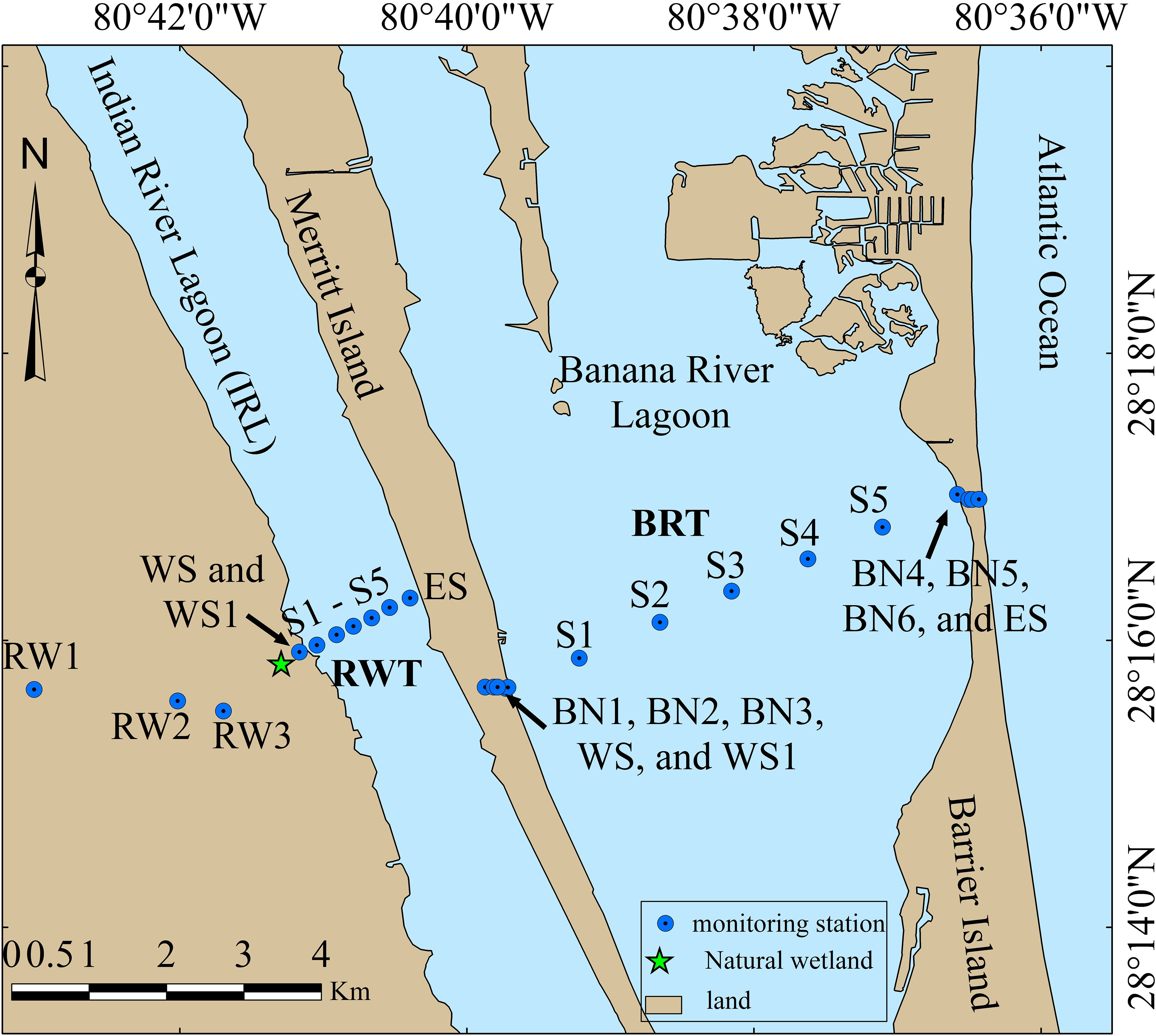
Figure 2 Details of onshore and offshore monitoring stations and the IRLS at BRT and RWT.

FIGURE 3

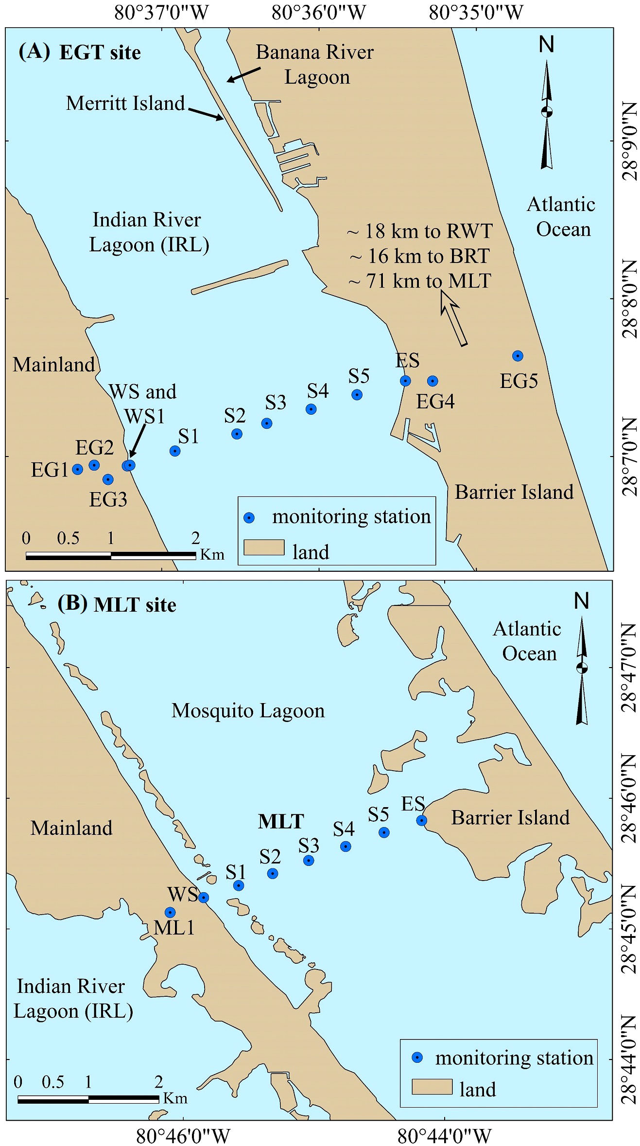
Figure 3 Details of onshore and offshore monitoring stations and the IRLS at (A) EGT; and (B) MLT.

The onshore monitoring stations were located on the mainland and the Barrier Island, and a single deep piezometer was installed at each onshore station of each transect. A total of seven offshore stations, each of which hosted a nest of a shallow and a deep piezometer, were installed equally spaced across the lagoon water body at each transect (Figure 4). The west and east shoreline stations are symbolized by WS and ES, respectively, while the rest of the offshore stations are symbolized by S1 through S5 (Figures 2, 3). The WS stations at the BRT, RWT, and EGT sites also included an extra deep piezometer symbolized as XD with a length of 6.7 m. Additional stations denoted by WS1 were also installed at the BRT, RWT, and EGT sites at 29 m, 19 m, and 34 m from the west shoreside, respectively (Figure 4). All WS1 stations hosted a nest of a shallow and a deep piezometer except that at the EGT site, which also included an XD and an additional deeper piezometer with a length of 8.5 m and denoted by XXD (Figure 4). The reason for increasing the number and depth of the piezometers near the WS stations was to increase the TGD measurement resolution near the west shore, where it is expected to be higher than that at other locations. The approximate distances from BRT, RWT, and MLT to EGT are 16 km, 18 km, and 71 km, respectively (Figure 3A).

FIGURE 4

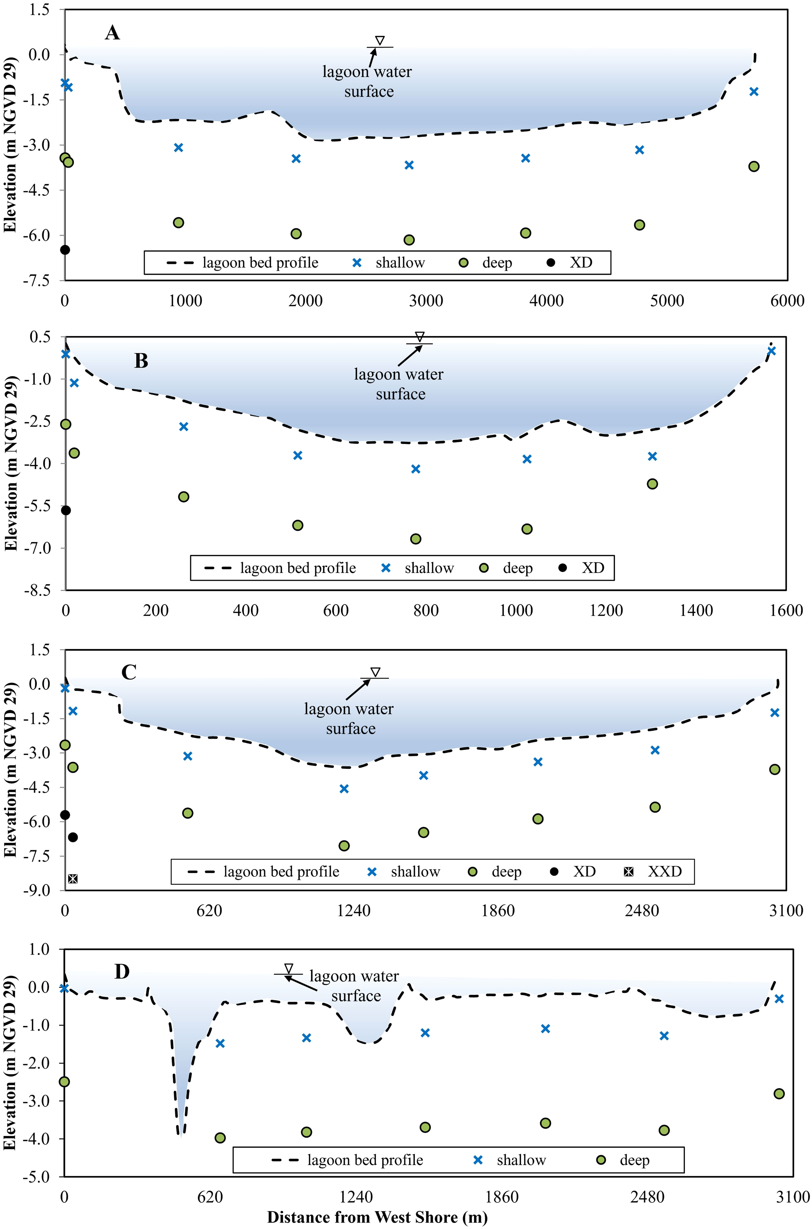
Figure 4 Bed profiles and locations of monitoring piezometers used for the measurement of groundwater hydraulic heads and salinity at (A) BRT; (B) RWT; (C) EGT; and (D) MLT.

3.2 Lagoon bed profiles

Profiles of the lagoon at each of the study transects were delineated by measuring the water depth at multiple locations along the transects. Water depth measurement was accomplished by inserting a surveying staff down the lagoon water at 28 to 45 locations until touching the bottom and taking a depth reading while traveling with a boat from shoreline to shoreline. The lagoon water surface elevation in the national geodetic vertical datum of 1929 (NGVD29) was determined by surveying the benchmarks and measuring the distance from the top surface of the benchmark to the water surface. The calculated surface water elevation was used to calculate the lagoon bed elevations in NGVD29 by subtracting the lagoon water depths measured along the transect from the surface water elevation. The lagoon bed elevations shown in (Figure 4) were determined during site characterization prior to data collection.

3.3 Data collection and sites investigations

Field data were acquired during five visits to each transect, including two visits in 2014 (June/July 2014 and September/October 2014) and three visits in 2015 (May/June 2015, June/July 2015, and September 2015). During every single visit to any of the transects, the sequence of data collection started from measuring the water table elevations in the onshore piezometers on the mainland or Merritt Island, surveying the benchmark on the west shoreline to determine the lagoon water surface elevation, measuring groundwater head and salinity and collecting groundwater samples for nutrient determination in the offshore stations, surveying the east shoreline benchmark to determine the lagoon water surface elevation, and finally, measuring water table elevations in the onshore stations on the Barrier Island. Groundwater level data collected from the onshore piezometers were used to obtain groundwater surface profiles, which were used as boundary conditions in the numerical models. Groundwater profiles on the mainland, Merritt Island, and Barrier Island were also employed to determine the locations of groundwater divides at each site. These determinations were accomplished by interpolating the measured groundwater elevations using GMS software v.6 (Aquaveo, 2011). Figures 5, 6 show some of the contour maps of groundwater elevations and the locations of groundwater divides obtained from the interpolation process. All contour maps were generated using a similar method; however, they are not all presented here for brevity. Data collection from all the offshore stations on any single visit at any of the transects usually took 4-5 hrs., during which, water surface elevation may change due to tidal action. This is the reason for using two benchmarks at each site: the one on the west shore, which was sampled at the beginning, and the other on the east shore, which was sampled at the end of the offshore data collection. Calculating the lagoon water surface elevation from the elevations of the surveyed benchmarks was accomplished as described in section 3.2 and was based on the average of the two benchmark measurements. Data collected from the offshore stations at each transect on any sampling visit included groundwater hydraulic heads and salinity from all deep and shallow piezometers, groundwater samples for nutrient determinations from all shallow piezometers, lagoon surface water salinity at all offshore stations, and samples for lagoon surface water nutrient determinations near the middle stations. Groundwater samples were obtained using a peristaltic pump that was kept running and pumping into a beaker, from which the salinity of the sample was continuously measured using a Yellow Springs Instruments (YSI) meter V85 until a constant salinity reading was obtained. After reaching a constant salinity reading, groundwater salinity was recorded and samples for nutrient determinations were stored in screw cap vials, labeled, and kept in an ice box for further laboratory work. The surface water salinity was simply measured by collecting a grab sample in a beaker and dipping the probe of the YSI into the beaker. The probe of the YSI was washed thoroughly using distilled water before each measurement.

FIGURE 5

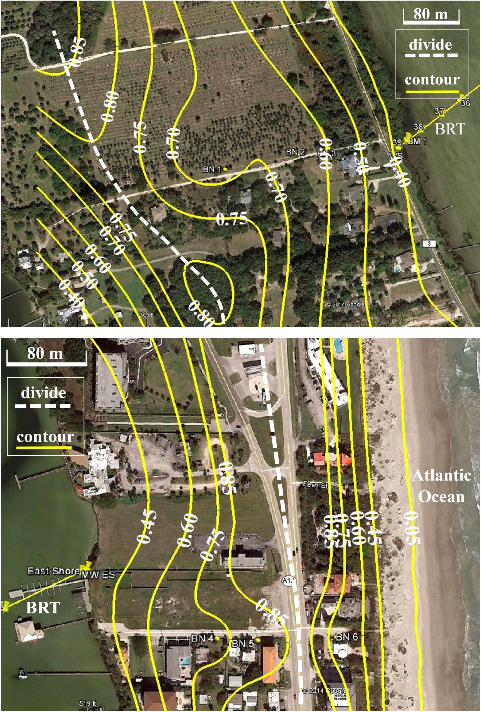
Figure 5 Contour maps of groundwater levels and locations of groundwater divides in Merritt Island (Top) and Barrier Island (bottom) at the BRT site.

FIGURE 6

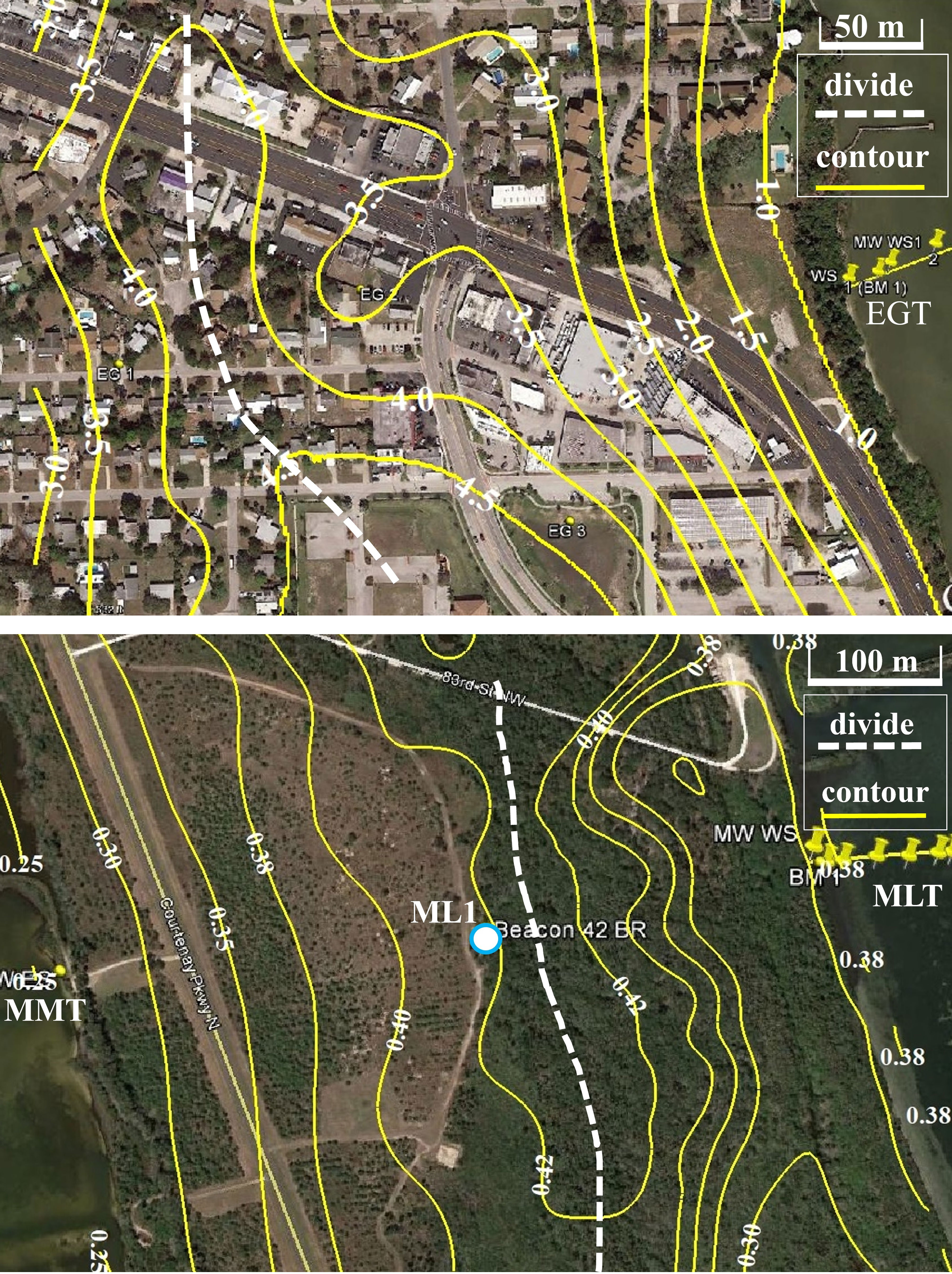
Figure 6 Contour maps of groundwater levels and locations of groundwater divides in the mainland at EGT site (Top) and the mainland at the MLT site (bottom).

3.4 Horizontal hydraulic conductivity

Horizontal hydraulic conductivity, K_h, of the saturated SUA below the lagoon was approximated at each site using Hazen’s empirical equation (Equation 1):

$\begin{array}{ll}{K}_h=C{\left(d_{\mathit{10}}\right)}^{\mathit{2}}& (1)\end{array}$

where d₁₀ is the effective diameter in (mm), and C is a dimensionless empirical constant = 1 (Uma et al., 1989).

The effective diameter of the lagoon bed sediments was obtained by developing grain size distribution curves. Soil samples of approximately 750 g each were collected from the top 30 cm of the lagoon bed for laboratory sieve analysis from five locations at BRT, EGT, and MLT, and three locations at RWT, uniformly distributed along the transects (Table 1). The average estimated values of K_h were ~14 m/d at MLT, ~20 m/d at BRT and EGT, and ~18 m/d at RWT. A K_h of ~15 m/d was used by previous modeling research works of the SUA at the eastern coast of Florida near the study sites (McGurk and Presley, 2002; Xiao et al., 2019), which falls well within the estimated range in our work.

TABLE 1

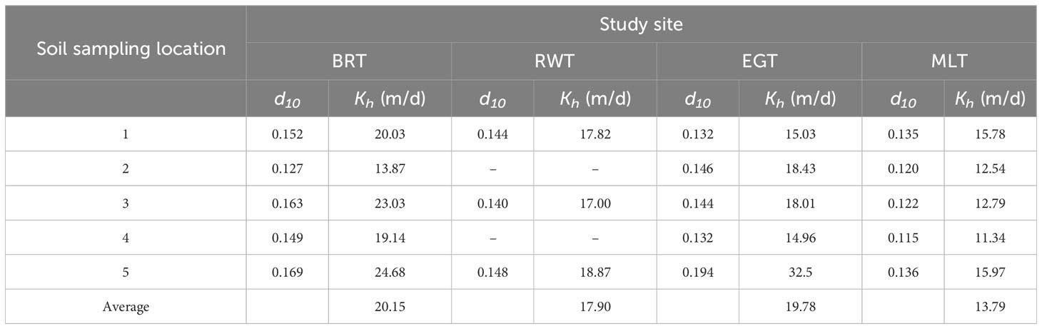
Table 1 Estimated horizontal hydraulic conductivity using sieve analysis.

3.5 Laboratory analytical methods

Dissolved inorganic nitrogen (DIN) is stated as the summation of nitrite + nitrate + ammonium (NO₂ + NO₃ + NH₄) concentrations, while dissolved inorganic phosphorus (DIP) is stated as the orthophosphate (PO₄) concentration. Concentrations of dissolved nutrients in groundwater and surface water were determined using a SEAL AutoAnalyzer 3 HR, following SEAL analytical methods G-172-96, G-171-96, and G-297-03 for (nitrite + nitrate), ammonium, and phosphorus concentrations, respectively. Concentrations of the sum (Nitrite + nitrate) were determined by reducing NO₃ to NO₂ in a cadmium-copper column. The original NO₂ and reduced NO₃ ions then react with sulfanilamide and N-(1-naphthyl)ethylenediamine di-hydrochloride aromatic amines in an acidic medium. Ammonium concentrations were obtained by treating the samples with alkaline phenol and hypochlorite to produce a blue color followed by the addition of sodium nitroprusside to intensify the color. Concentrations of DIP in the form of PO₄ were measured using the ammonium molybdate method in which, the PO₄ ions react with ammonium molybdate, and the resulting phosphomolybdenum complex is reduced in an acid medium to form a blue color that is measured by spectrophotometry. The respective detection limits for the (NO₂ + NO₃), NH_4, and PO₄ determination methods were 0.004 mg/L, 0.002 mg/L, and 0.003 mg/L. The laboratory experiments were duplicated ensuring identical conditions and the margin of error on the replicates was< 5%.

3.6 Determination of TGD and nutrient loads

Calculating the total simulated TGD and estimating its DIN and DIP loads were accomplished by discretizing each of the transects into multiple sections, with each section housing one offshore monitoring station and representing the area of influence of that station. For example, as shown in Table 2, which presents the calculations at EGT for the September 2015 data, was discretized into eight sections as there are eight offshore monitoring stations along the transect (Figures 3A, 4C). The width of each section was determined as the sum of half the distances between adjacent stations. For example, the width of Section 4 (Table 2) is the sum of half the distance between stations S2 and S1 and half the distance between stations S2 and S3. The TGD rates for each section, shown in Table 3, were obtained from the numerical models, and the total TGD rates were calculated as the sum of all TGD rates of the sections. The DIP and DIN loads for each section were calculated by multiplying the corresponding TGD values by the measured concentrations, and the total DIP and DIN loads for the entire transect were obtained by summing the corresponding nutrient load values for the eight sections, as documented in Table 2. Groundwater seepage rates and the associated nutrient loads were also calculated for the near-shore zones using the nutrient concentrations measured at the WS stations. Calculations similar to those in Table 2 were conducted for the entire width and for the near-shore zones of each transect on each of the five sampling visits.

TABLE 2

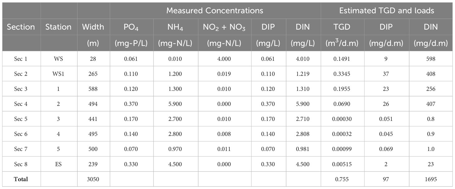
Table 2 Seepage and Nutrient Loading Calculations at the EGT Site in September 2015.

TABLE 3

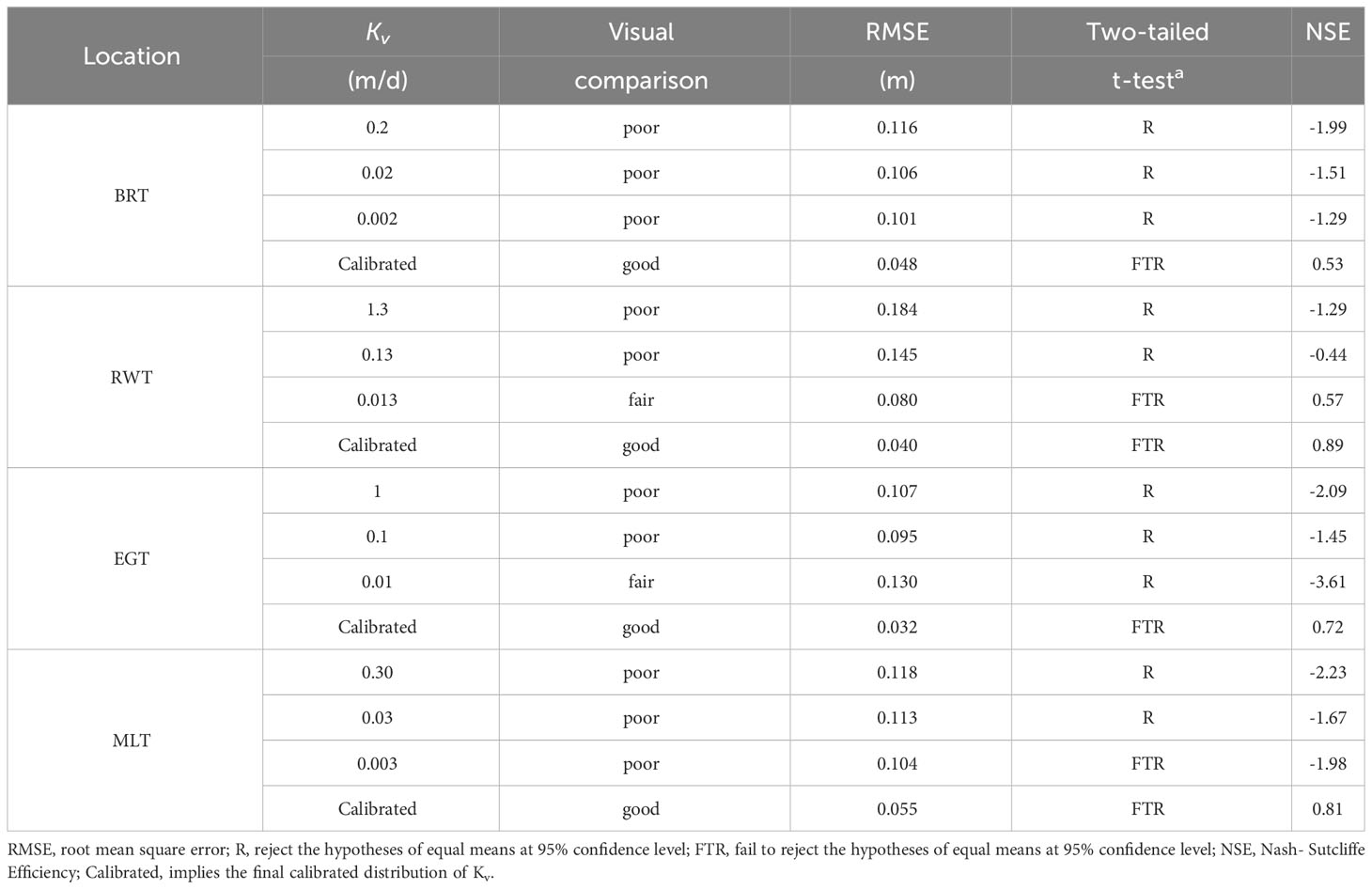
Table 3 Sensitivity analyses and model calibration statistics.

3.7 Effect of recharge through Hawthorn formation

As stated previously, the main analysis described in the previous sections assumed that the Hawthorn Formation was an impermeable surface since the hydraulic conductivity of this formation is relatively low. However, at all four of the study transects, the piezometric surface of the confined aquifer below the Hawthorn Formation is higher than the water table elevation in the unconfined aquifer above the Hawthorn Formation which indicates that there may be an upward recharge from the confined aquifer into the unconfined aquifer through the Hawthorn Formation. To investigate the effect of potential recharge from the Hawthorn Formation, the upward recharge rate was estimated using Darcy’s equation (Equation 2):

$\begin{array}{ll}Q=KA\Delta h/\Delta z& (2)\end{array}$

where Q is the recharge rate from the Hawthorn Formation to the unconfined aquifer per unit length of the shoreline, K is the hydraulic conductivity of the Hawthorn Formation, A is the area of cross-section of the transect with unit length, Δh is the difference in height between the piezometric surface and the water table elevation in the unconfined aquifer, and Δz is the thickness of the Hawthorn Formation. The parametric data for K, Δh, and Δz were obtained for EGT, RWT, and BRT from the maps and information provided by the St. John’s River Water Management District (Berber, 2017). Similar data for MLT were not available. The analysis was conducted with the calculated recharge and the results were compared with those obtained without recharge.

3.8 Graphical processing and statistical analyses of data

Graphical processing of data was accomplished using ArcGIS (version 10.8, ESRI, Inc., Redlands, California, USA) and Microsoft Excel (Microsoft Corporation, 2016). Statistical analyses including one-way ANOVA were carried out using Minitab (version 21.4.1, Minitab, LLC). One-way ANOVA coupled with Tukey’s test was performed to determine if there were statistically significant differences between multiple independent groups and to identify which groups were different in a one-step comparison assuming equal variances. Multiple groups of data were considered not significantly different when p-value was greater than 0.05 (significance level, α). When p-value< α, the alternative hypothesis that the groups were different was accepted, and Tukey’s test identified these differences by designating different groups by different letters and similar groups by similar letters.

4 Numerical models

4.1 Models description

Numerical simulations of groundwater flow and transport were performed using the finite difference code SEAWAT V4.0 (Langevin et al., 2008) within the pre-processing and post-processing environment of Groundwater Vistas V6.0 (Environmental Simulations, Inc., 2011). SEAWAT was chosen for its ability to efficiently mimic the variable-density flow and transport environment in the study area. The way SEAWAT solves problems is by coupling MODFLOW2000 (Harbaugh et al., 2000), for solving the groundwater flow equation in the three-dimensional space (Equation 3), with MT3DMS (Zheng and Wang, 1999), for solving the solute transport equation (Equation 4), in an iterative manner (Al-Taliby and Pandit, 2017). The coupling of Equations 3 and 4 is accomplished internally in SEAWAT through an equation of state (Equation 5).

$\begin{array}{ll}\begin{array}{c}\frac{\partial }{\partial x}\left[\rho K_x\right(\frac{\partial h}{\partial x}\left)\right]+\frac{\partial }{\partial y}\left[\rho K_y\right(\frac{\partial h}{\partial y}\left)\right]+\frac{\partial }{\partial z}\left[\rho K_z\right(\frac{\partial h}{\partial z}+\left(\frac{\rho -{\rho }_f}{{\rho }_f}\right)\frac{\partial Z}{\partial z}\left)\right]\\ =\rho S_f\frac{\partial h}{\partial t}+\theta \frac{\partial \rho }{\partial C}\frac{\partial C}{\partial t}-{\rho }_s{q}_s\end{array}& (3)\end{array}$

$\begin{array}{ll}\frac{\partial C}{\partial t}=\mathit{\nabla }.(D.\mathit{\nabla }C)-\mathit{\nabla }.\left(vC\right)-\frac{q_s}{\theta }{C}_s& (4)\end{array}$

$\begin{array}{ll}\rho ={\rho }_f+\frac{\partial \rho }{\partial C}C& (5)\end{array}$

where ρ is water density at salt concentration C; h is the equivalent freshwater hydraulic head; ρ_f is freshwater density; ρ_s is the density of seawater; Z is elevation head; K_x, K_y, K_z are equivalent freshwater hydraulic conductivities in the three coordinate directions; S_f is specific storage; q_s is the volumetric flow rate of sources and sinks per unit volume of the aquifer; θ is effective porosity; t is time; D is hydrodynamic dispersion; v is linear fluid velocity; C_S is salt concentration in the ocean; $\frac{\partial \rho }{\partial C }$ is the slope of fluid density and concentration.

Domains of the numerical models in this study extended over 2D vertical planes with lateral dimensions of BRT, RWT, EGT, and MLT of 6270 m, 2733 m, 4940 m, and 4391 m, respectively (Figure S1, Supplementary Material). All models span vertically downwards to the Hawthorn Formation, which ranged from 28.5 m NGVD 29 at MLT to 44.0 m NGVD 29 at BRT and RWT. The finite difference grids of the model domains of all four transects were discretized into a single row of 1 m length parallel to the lagoon’s shoreline. In the lateral direction, the grids of BRT, RWT, EGT, and MLT contained 175, 108, 156, and 160 columns, respectively, with respective column widths ranged from 5 to 50 m, 5 to 50 m, 2 to 100 m, and 2 to 50 m. In the vertical direction, the model domains for BRT, RWT, EGT, and MLT contained 48, 42, 41, and 36 layers, respectively, with layer widths ranging from 0.25 to 3.00 m. The finite difference grid was refined at some locations to ensure that there were nodes at the measurement stations to conveniently compare the modeled and measured hydraulic head values. Grid refinement also aided in the precise layout of the lagoon bed profiles (Figure 4) in the numerical grids.

Referring to (Figure S1), boundaries AB and CD that represent the mainland or Merritt Island and the Barrier Island were modeled as specified head (Dirichlet) boundaries. Piezometric heads used at these boundaries were set equal to the water table elevations measured at the onshore monitoring wells. The water table elevations are from the top of the Hawthorn Formation. The specified concentration at boundaries AB and CD was zero because there is freshwater at these boundaries, which typically has a negligible salt concentration. Boundary BC represents the lagoon bed and is also a Dirichlet boundary, and the piezometric heads used at this boundary were set equal to the measured lagoon water levels. All grid cells at the boundary BC were assigned a constant salt concentration, C_L, which is defined as the normalized average lagoon surface water salinity and is calculated using Equation 6:

$\begin{array}{ll}{C}_L=\frac{C_m}{C_s}& (6)\end{array}$

where C_m is the average lagoon salinity measured at the offshore stations, C_s is defined previously and is equal to 35. At all transects except RWT, the domain extended to the Atlantic Ocean as shown in Figure S1. Therefore, the boundary DE in all models except the RWT represented the ocean and was simulated as a Dirichlet boundary. The piezometric heads were assigned as the depth to the top of the Hawthorn Formation in NGVD 29, which is located at an elevation of 44, 44, 40, and 28.5 m below NGVD 29 at BRT, RWT, EGT, and MLT, respectively. At RWT, the domain extended to the water table divide on the barrier island (Figure S1, Supplementary Material), and at this transect, boundary DE was simulated as an impermeable or no-flow boundary. In all cases where the boundary DE represented the oceanside, the boundary cells were assigned a constant salt concentration equal to a seawater normalized salinity of 1. Boundary EF lies at the top of the Hawthorn Formation, which was initially considered as an impermeable layer. Therefore, initially, this boundary was also considered to be an impermeable or no-flow boundary. In subsequent analysis, the Hawthorn Formation was considered as a recharge boundary that transmitted groundwater from the artesian aquifer into the unsaturated aquifer. The estimation of groundwater recharge through this boundary is described in a subsequent section. During analyses where this boundary was considered to be a recharge boundary, the boundary condition for concentration at this boundary was set equal to the estimated normalized concentration of the water coming up the Hawthorn Formation. Boundary FA represented the water table divide at all four transects and was therefore modeled as a no-flow boundary, and no saltwater could flow across this boundary.

In terms of the initial conditions used in the models, the entire domains of all models were assigned values equal to the unconfined aquifer height for the piezometric head (Figure S1, Supplementary Material), while the initial saltwater concentration was set to zero. In other words, it was assumed that initially there was only freshwater in the entire domain except for BC, where initial salt conditions were assigned a salt concentration equal to C_L (Equation 6). All simulations were run in transient stress periods using the implicit finite difference method with the generalized conjugate gradient (GCG) solver until steady states were reached.

4.2 Models calibration

The finite difference models at each transect were calibrated and validated before estimating the seepage and associated nutrient fluxes delivered to the IRLS. Ahead of the calibration process, the groundwater hydraulic heads measured at the offshore stations were first converted into equivalent hydraulic heads and then interpolated using the inverse distance weighted interpolation (INVD_W) method in the groundwater modeling system (GMS) software v.6 (Aquaveo, 2011). Groundwater equipotential contours below each transect were generated using the INVD_W for each sampling visit (Figures S2B, D, S3B, D, S4B, D, S5B, D in Supplementary Materials). The calibration was initiated by conducting model sensitivity analyses, in which a single vertical hydraulic conductivity, K_v, was assigned to each model. Sensitivity analyses showed that hydraulic head distributions below the lagoon are primarily sensitive to K_v (Table 3); therefore, K_v was considered as the principal calibration parameter. The modeled and observed hydraulic heads were compared on the basis of multiple measures, including visual comparison of equipotential contours, root mean square error (RMSE), two-tailed student t-test, and Nash-Sutcliffe Efficiency coefficient (NSE) (Nash and Sutcliffe, 1970), which are among the most commonly used statistical tools to quantitatively evaluate the goodness of model calibration. In the t-test, the null hypothesis of equal means was considered failed to reject (FTR) at p-values > 0.05 (95% confidence level); otherwise, the hypothesis was rejected (R). As a result, a FTR implies sufficient calibration, whereas R implies poor calibration. A perfect model would have an NSE = 1; however, the general descriptors used for model calibration based on NSE are NSE< 0.5 (unsatisfactory), 0.5< NSE<0.7 (satisfactory), and NSE > 0.7 (good) (Goodarzi et al., 2020). While the primary goal of using RMSE in evaluating model calibration is to minimize the numerical value of this statistical measure, there is no definitive RMSE threshold that can definitively designate a prediction as good or poor. Thus, designating model performance as “good” or “poor” based on RMSE remains subjective. Because the RMSE value depends on the specific measurement units employed, there is no universal value that holds across all applications and data scales. Anderson et al. (2015) stated that RMSE values less than 10% of the mean of the measured target values may indicate that a model is acceptable for most purposes. In each model calibration run, the relevant average K_h values presented in Table 1 were assigned to the entire domain of each respective model. Calibration was achieved in two phases. Initially, the calibration was automated using model-independent nonlinear parameter estimation (PEST) software (Doherty, 2010). Finally, the obtained PEST-calibrated K_v distributions were refined manually using the trial-and-error method. It was only considered that the calibration was sufficient when all four measures indicated a good or satisfactory match between the simulated and observed data. The calibrated parametric values were used to validate the model by comparing the predictions with measured field data on subsequent dates.

5 Results and discussion

5.1 Calibrated and validated models

Data presented in Table 3 clearly show the sensitivity of the models to K_v when it was changed from 0.2 to 0.002, 1.3 to 0.013, 1.0 to 0.01, and 0.3 to 0.003 for BRT, RWT, EGT, and MLT, respectively. These results also demonstrate the importance of relying on multiple measures to calibrate the models instead of a single measure. This is because some of those measures were noticed to indicate sufficient calibration, whereas the other measures indicated poor or insufficient calibration. For example, at the BRT, when using a K_v of 0.002 m/d, a small RMSE value was obtained (which may indicate sufficient calibration) even though the visual comparison, t-test, and NSE value still indicated poor calibration. In addition, when a K_v of 0.003 m/d was assigned to the domain of the MLT model, both the RMSE and t-test indicated sufficient calibration, whereas the visual comparison and NSE did not agree with this result. The final runs of each of the models with the calibrated K_v distributions clearly show how all four calibration measures agreed with the goodness of fit between the modeled and observed results when good visual comparisons, small RMSE values, FTR t-test results, and NSE > 0.5 were obtained. The calibration process showed that while the vertical hydraulic conductivity was spatially variable, the predominant values were 0.020 m/d at BRT, 0.014 m/d at RWT, 0.010 m/d at EGT, and 0.013 m/d at MLT. The calibration of BRT, RWT, EGT, and MLT was accomplished using the July 2015, July 2014, June 2014, and July 2014 sampling visit data to each of the sites, respectively. The calibration was validated by applying different stress periods to the calibrated models obtained from October 2014, June 2015, June 2015, and July 2015 sampling visit data to each of the sites for the BRT, RWT, EGT, and MLT, respectively. The comparisons between the simulated and observed groundwater equipotential contours below the lagoon at all four sites for both the calibration and validation runs clearly indicate good performance and an efficient calibration procedure for the numerical models (Figures S2-S5, Supplementary Material).

5.2 Lagoon water and groundwater salinity levels

The Box and Whisker plot (Figure 7A) displays the lagoon water salinity patterns during the five field visits between June 2014 and September 2015. Noticeable temporal variations in lagoon salinity exist at EGT, RWT, and BRT with values ranging from (19 to 28.3), (20.9 to 32.9), and (22.3 to 30.8), respectively. Although RWT exhibited higher temporal variation than EGT and BRT, the medians of lagoon salinity at these three transects were relatively similar. Temporal differences in the lagoon salinity at each transect are primarily due to a combination of freshwater entering the lagoon through direct rainfall, surface water runoff, and groundwater flow. The lagoon water at MLT remained saline throughout the year, and the salinity at this transect ranged from 29.7 to 32.2 with smaller temporal variation than the rest of the study sites. As a spatial comparison, the minimum salinity at the MLT is higher than the maximum salinity at the EGT and higher than the third quartile of all three transects (Figure 7). Phlips et al. (2002) reported similar long-term high salinity levels in the Mosquito Lagoon in their study of phytoplankton dynamics. This might be attributed to the MLT’s proximity to the Ponce De Leon Inlet and perhaps to the narrow watershed area on the mainland side. A one-way ANOVA with a Tukey’s multiple comparisons test was conducted on the data presented in Figure 7A to compare lagoon salinity patterns between sites at a 95% confidence level. Analysis revealed the salinity patterns at the MLT site were significantly divergent from those observed at both the EGT and RWT sites. The Tukey’s test also indicated water salinity levels at the BRT site exhibited comparable values to the other three locations evaluated. In summarizing, while salinity trends differed distinctly between MLT relative to EGT and RWT based on the one-way ANOVA, BRT salinity patterns closely resembled the overall tendencies seen across all locations measured according to the results of this statistical technique.

FIGURE 7

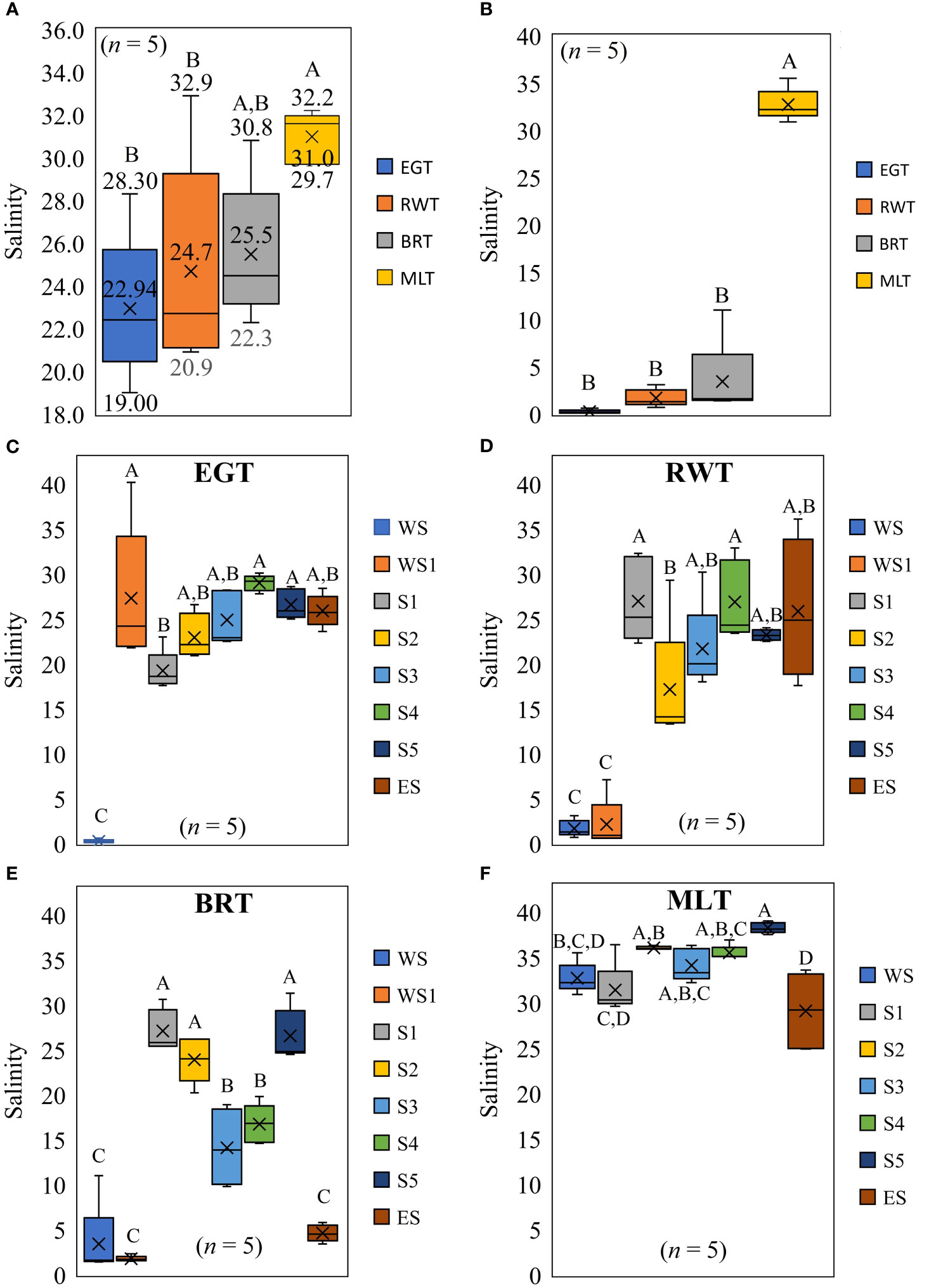
Figure 7 Box and Whisker plots of salinity measured over the five sampling visits including: (A) lagoon surface water salinity measured at the four transects, (B) groundwater salinity measured at the WS stations at the four transects, (C) groundwater salinity measured at all offshore stations at EGT, (D) groundwater salinity measured at all offshore stations at RWT, (E) groundwater salinity measured at all offshore stations at BRT, and (F) groundwater salinity measured at all offshore stations at MLT. The numbers in graph (A) are the maximum, average, and minimum values from top to bottom and the dark lines inside the boxes are the medians. EGT, RWT, BRT, and MLT stand for Eau Gallie transect, River Walk transect, Banana River Transect, and Mosquito Lagoon transect, respectively. WS, WS1, S1, S2, S3, S4, S5, and ES stand for westshore station, near westshore station, offshore stations no.1 through 5, and eastshore station. The letters A through D are assigned to tested groups by the one-way ANOVA Tukey test.

Analysis of the data presented in Figure 7B revealed very low groundwater salinity concentrations at the EGT, RWT, and BRT monitoring sites at the WS stations, with particularly minimal levels ranging from 0.1 to 0.7 recorded at EGT and RWT. In stark contrast, the WS station at MLT exhibited exceedingly high salinity (up to 35) with negligible variation across the entire sampling period. These remarkably low salinity readings near the WS stations at the other three locations are suggestive of higher TGD rates on the west shorelines owing to the higher hydraulic gradients governing flow dynamics in those regions. Statistical analysis via one-way ANOVA with Tukey’s test demonstrated that the salinity distribution at the WS station of the MLT was significantly different compared to all other three sites, which exhibited comparable values. Therefore, while groundwater salinity levels at the EGT, RWT, and BRT WS stations were remarkably low and similar, MLT uniquely presented very high and markedly different concentrations according to this inferential analysis. Figures 7C-F explore the spatial and temporal variations in groundwater salinity levels across the entire cross-sectional width of each of the four sites. Statistical analysis via ANOVA with Tukey’s test revealed that at EGT (Figure 7C), salinity levels at stations WS1 through ES maintained consistently elevated concentrations that diverged significantly from readings at WS but exhibited some similarities among each other. The recorded subsurface salinities offshore at RWT (Figure 7D) exhibited comparable behavior to that at EGT, except that station WS1 at RWT presented a variation resembling that at WS per the statistical assessment. Across the entire BRT transect (Figure 7E), groundwater salinity variations near the lagoon shorelines at stations WS, WS1, and ES were similar, whereas the internal stations differed conspicuously from the boundary stations while sharing certain commonalities. Distinct from the other three sites, MLT (Figure 7F) exhibited consistently high subsurface salinities that remained statistically uniform across the entire cross-section evaluated. Therefore, spatial and temporal trends in salinity manifested diversely between sites according to Tukey’s quantitative analysis.

5.3 Flow direction and salt transport

Figure 8 shows the simulated groundwater velocity vectors and salt transport in the subterranean estuaries below the four transects. Groundwater from the mainland initially flows downward and then begins to flow in an upward direction into the lagoon at the four transects. On the ocean boundaries, saline groundwater intrudes the bottom of the aquifer, mixes with fresh groundwater, and recirculates back to the ocean at the upper region of the boundary. Figure 8 also shows that saltwater from the lagoon moves downward into the unconfined aquifer at all four transects. The presence of the Atlantic Ocean on the east side of the region at EGT, BRT, and MLT also causes typical saltwater intrusion from the ocean into the aquifer, although this intrusion is not extensive. A similar saltwater intrusion is not evident at RWT because the right-hand boundary of this transect is the water table divide on the Barrier Island and not the Atlantic Ocean. The upward motion of the groundwater carries nutrients into the lagoon along the transects.

FIGURE 8

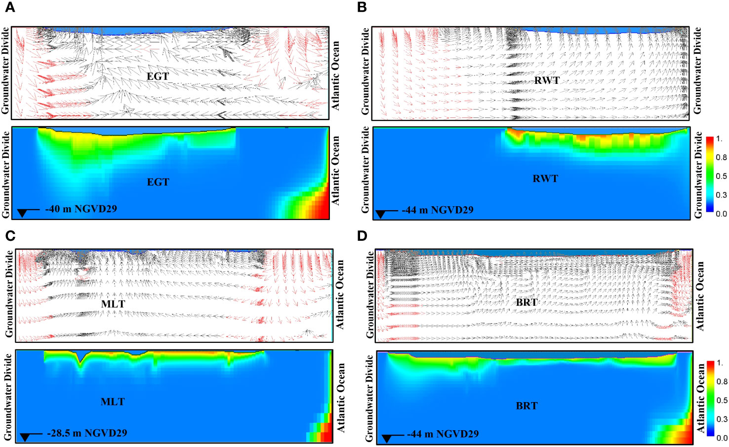
Figure 8 Ground water flow direction and salinity distributions in the subterranean estuary at (A) EGT; (B) RWT; (C) MLT; and (D) BRT. Arrows in the top graphs indicate the direction of ground water flow and the color flooded graphs in the bottom show saltwater distribution below the lagoon and from Ocean; blue = freshwater (C= 0) and red = saltwater (C= 1.0) as indicated by the color bar.

5.4 Spatial distribution of groundwater flow

Three interesting findings can be viewed when looking at the model-predicted spatial distribution of groundwater flows based on measurements taken in June/July 2014 along each of the four transects, as shown in (Figures 9A-D). In these figures, the distances are from the shoreline on the mainland side. First, the results showed that while the majority of the groundwater comes from the mainland and enters the lagoon near the shoreline, a small volume of groundwater is transported into the lagoon throughout the transects. A second observation was that the region near the mainland shoreline receiving a larger volume of groundwater, termed the “near-shore” zone in this paper, was quite a bit wider than the traditional “nearshore”. For example, this region extended to distances of 198 m, 157 m, 165 m, and 40 m at EGT, RWT, MLT, and BRT, respectively (Figures 9A-D). The lengths of these near-shore zones are 6.5, 10.0, 5.4, and 0.7% of the entire width of the transects, respectively. The near-shore zones are different from the traditional “near-shore” as the water in these zones can be either fresh water or brackish water, whereas the traditional nearshore zone only has fresh water. A third observation is that there are some narrow “hot spots” along the transect where the groundwater flow into the lagoon suddenly increases. For example, there are “hot spots” at distances of 500 m, 1500 m, 2500 m, and 2900 m from the mainland shoreline along the MLT (Figure 9C). A similar “hot spot” occurs at 1000 m at the EGT. These “hot spots” coincide with the relatively higher vertical hydraulic conductivities in these regions and remain consistent over time (Figure S6, Supplementary Material). The predicted directions of flow (Figure 8) and the spatial distribution of the TGD at the four transects (Figure 9) showed that the TGD occurs across the IRLS and may not be constrained to a near-shore region.

FIGURE 9

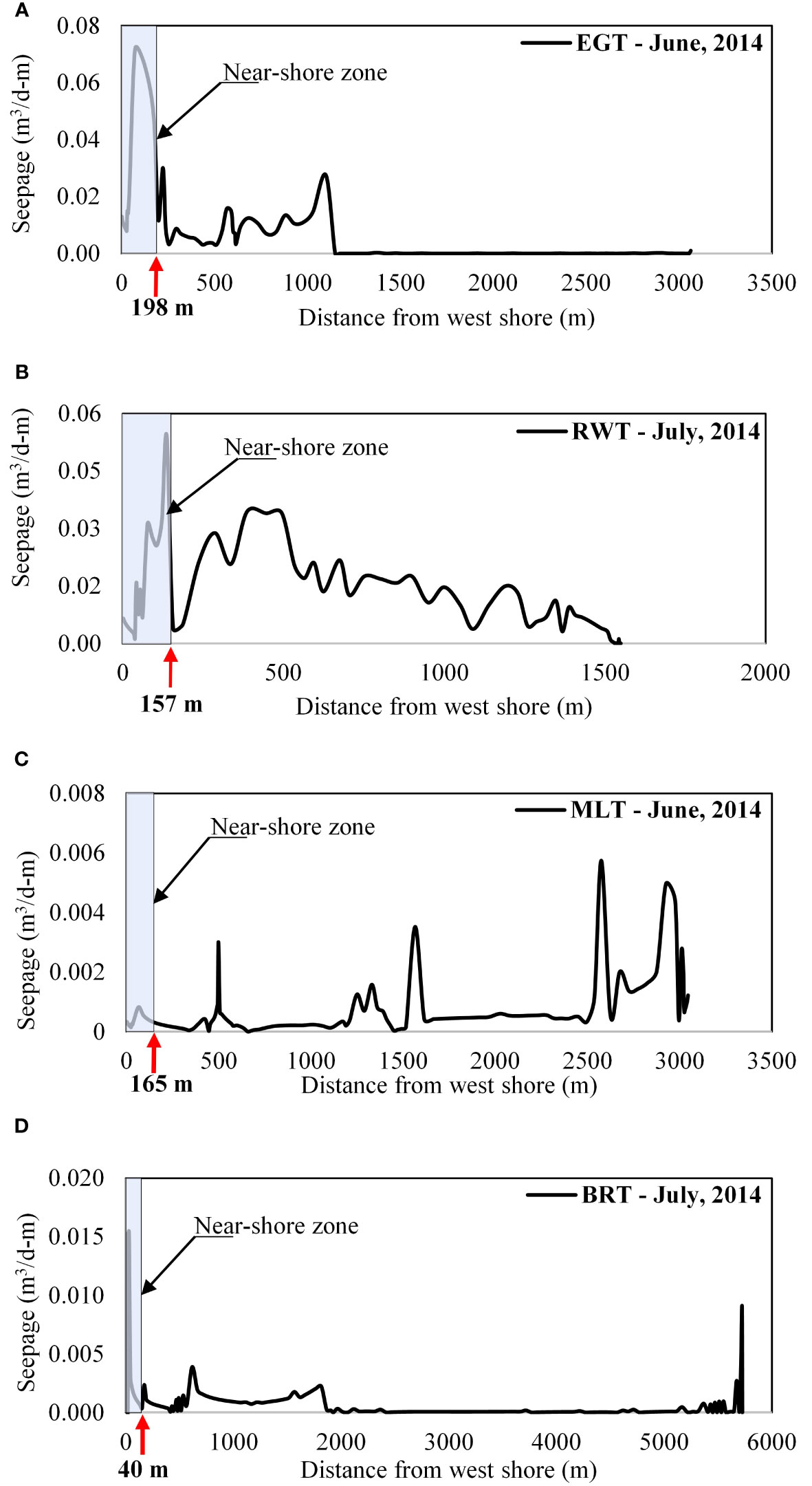
Figure 9 Simulated spatial groundwater discharge (cubic meters per day per meter of lagoon shoreline) below the lagoon at (A) EGT; (B) RWT; (C) MLT; and (D) BRT. Red arrows indicate the extent of near-shore zones.

5.5 Measured nutrient concentrations

The groundwater and lagoon surface water content of the total measured phosphorus concentration (DIP) was assumed to be equal to the soluble reactive phosphate (PO₄) concentration and the total measured nitrogen concentration (DIN) was determined by adding the concentrations of ammonium (NH₄) and nitrite + nitrate (NO₂ + NO₃) and the results are presented in Figure 10. Nutrient data used in developing Figure 10 were obtained by averaging the nutrient concentrations measured over the transect width in the offshore stations on any sampling visit to obtain a single average for that visit. Thus, n = 5 for each graph in Figure 10. Elevated ammonium concentrations in groundwater were observed at all sites, with the highest average of 268.6 μM recorded at MLT. The BRT site is in the second-highest position in ammonium concentration with an average of 132.8 μM and a maximum that exceeds 225 μM over the entire sampling program. The time-averaged NH₄ distributions in groundwater at the EGT and RWT look very similar in range and average (Figures 10A-C). In addition to elevated values, large temporal variations were observed in the ammonium distributions at all sites (Figures 10A-D). The highest average concentration of 42.6 μM of (NO₂ + NO₃) in groundwater with obvious temporal variation was recorded at the EGT site, unlike the other three sites, where significantly lower and very temporally invariant levels ranging from (0.6 to 3.9 μM) are measured. Groundwater phosphorus concentrations were significantly lower than ammonium concentrations at all sites, with the highest average concentration of 18.7 μM recorded at MLT (Figures 10A-D).

FIGURE 10

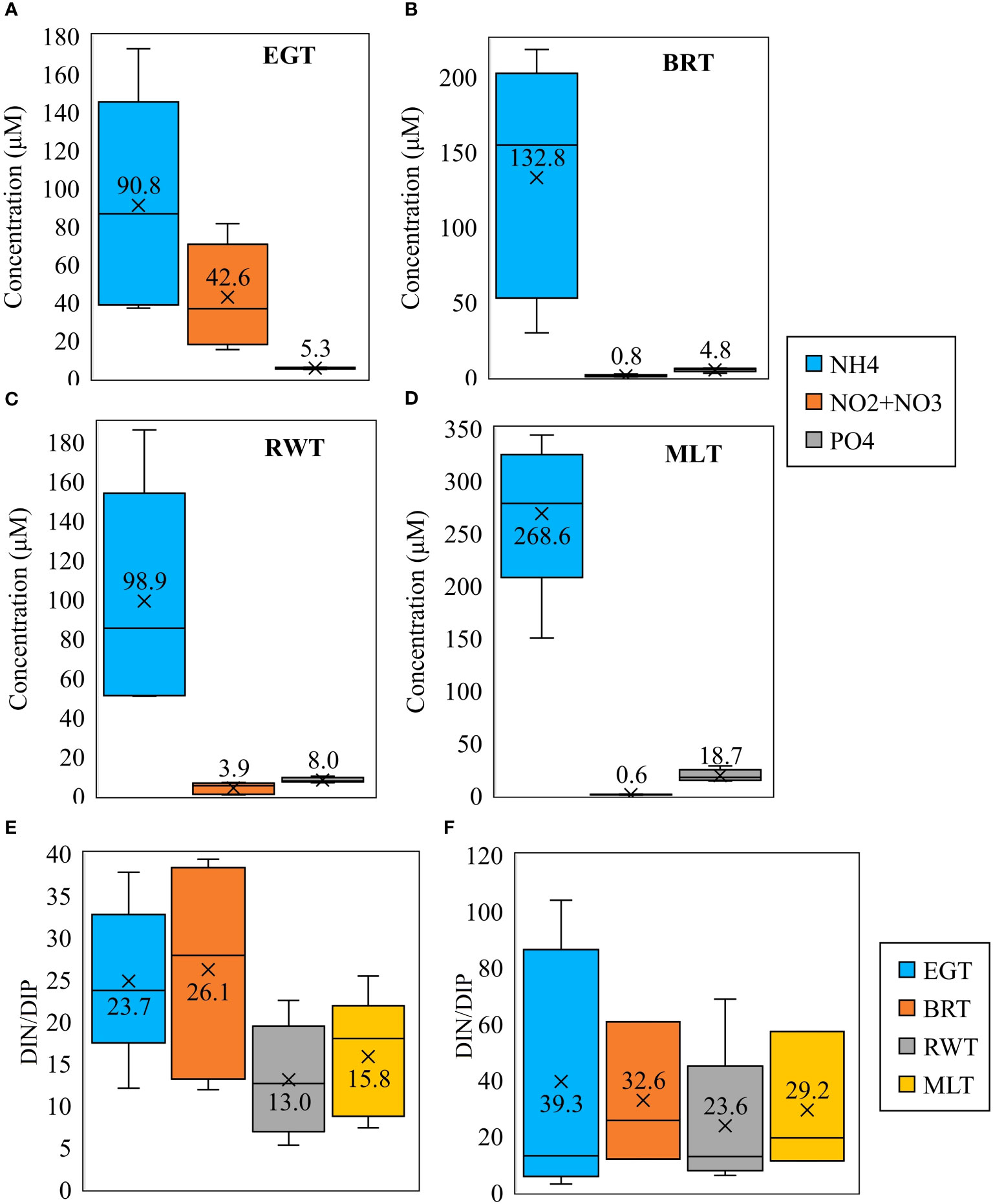
Figure 10 Box and Whisker plots of the time-averaged measured nutrients through the five sampling visits including (A) measured nutrient concentrations at EGT, (B) measured nutrient concentrations at BRT, (C) measured nutrient concentrations at RWT, (D) measured nutrient concentrations at MLT, (E) N/P molar ratio in groundwater below each of the transects, and (F) N/P molar ratio in the lagoon surface water. Numbers inside the boxes imply average values.

Elevated ammonium concentrations may reflect anthropogenic contamination received by the lagoon from inland sources such as fertilizers and septic tanks. For example, EGT, RWT, and BRT are all located offshore of developed areas with residential or commercial land uses. The presence of mangroves on the shorelines of the MLT and BRT and the presence of a natural wetland just onshore of the RWT (Figure 2) may have a synergistic effect that elevates the NH₄ concentration and reduces the (NO₂ + NO₃) concentrations measured at these sites. Mangroves and wetlands play a significant role in biogeochemical reactions by assimilating nitrate and significantly reducing its concentration by denitrification, where nitrate is reduced to N₂ gas by microorganisms (Erler et al., 2014), and by dissimilatory nitrate reduction to NH₄ (Decleyre et al., 2015). Mangroves are absent on the shoreline of the EGT, which may explain the higher nitrate/nitrite concentrations at the site than at the other three sites. Remineralization reactions catalyzed by microorganisms produce iron and manganese oxides in the sediments with high affinity to adsorb orthophosphate from groundwater into their surfaces and significantly reduce its transport in groundwater (Charette and Sholkovitz, 2002), which may explain the lower PO₄ concentrations at all sites over the entire study period (Figures 10A-D). CaCO₃ can also act as a scavenger of phosphorus and immobilize it through co-precipitation (Cable et al., 2002). Unlike the other three sites, the MLT is not connected to the anthropogenically impacted mainland. Thus, the highest NH₄ concentration and lowest (NO₂ + NO₃) concentration observed at MLT compared with the other three sites (Figures 10A-D) may be attributed to the in-situ mineralization of organic matter in the sediments, which increases with slow SGD rates. Transformations of SGD-derived nutrients and organic matter remineralization (denitrification, dissimilatory nitrate reduction to ammonium, and phosphorus adsorption and co-precipitation) increase in sandy sediments with slow SGD (Beck et al., 2017; Reckhardt et al., 2017). This may be supported by the slowest specific discharge at the MLT predicted by the numerical models, as discussed in section 5.6.

To evaluate the potential effect of nutrients on the lagoon integrity, variations in molar DIN/DIP ratios in groundwater and lagoon surface water at the four sites over the five sampling episodes were determined and compared to the Redfield ratio (Redfield, 1958), as shown in (Figures 10E, F), respectively. The Redfield ratio indicates the limitation of primary productivity through nitrogen or phosphorus limitation in coastal waters (Ptacnik et al., 2010). A Redfield ratio (DIN/DIP) that exceeds 16/1.0 stimulates the growth of harmful algal blooms (Santos et al., 2021). Figure 10E shows that the Redfield ratio in the porewater was exceeded differently at the four sites, with the maximum values exceeding 16 at all sites. The highest average porewater DIN/DIP ratios of 26.1 and 23.7 were recorded in BRT and EGT, respectively, with large temporal variations between ~ 12 and 38. At the RWT and MLT sites, the average porewater DIN/DIP molar ratios were near the standard ratio of 16/1.0, although the ratio was exceeded to up to ~ 23 at the RWT and 25 at MLT during some sampling events (Figure 10E). The high DIN/DIP ratios in the porewater are reflected in the nutrient ratios of the lagoon surface water, which is the medium where the primary productivity occurs. DIN/DIP molar ratios in the lagoon water were the highest at EGT with a value of 39.3, followed by the BRT with a ratio of 32.6, then at MLT with a ratio of 29.2, and finally at RWT with a ratio of 23.6 (Figure 10F). It can be inferred from (Figure 10F) that the lagoon is nitrogen enriched at the four sites with a high potential to encourage the blooming of harmful algae. Similar results were obtained in a previous investigation at a transect near Mims, termed MMT, at the far north end of the IRL (Figure 1), where DIN/DIP ratios in the porewater and lagoon surface water were found to surpass the Redfield ratio by a factor of 48 and 4, respectively (Al-Taliby and Pandit, 2023).

5.6 Estimated TGD and loads of DIN and DIP

Since EGT and RWT are connected to the mainland, whereas BRT and MLT are not, it was expected that the groundwater inflow into the lagoon would be the highest at these transects. The model predictions were consistent with these expectations. During the five visits, the modeled daily groundwater seepages in m³/d per meter of shoreline at EGT, RWT, BRT, and MLT ranged from (0.62 to 0.84), (0.69 to 0.85), (0.13 to 0.29), and (0.06 to 0.138), respectively (Figure 11A). The model-predicted average daily groundwater seepages in m³/d per meter of shoreline at EGT, RWT, BRT, and MLT were 0.74, 0.77, 0.18, and 0.09, respectively. The highest seepage rate is predicted to occur at RWT, a result that agreed with what we observed during the field work when the groundwater overflowed from the WS piezometer, and an extension pipe was added to take the head measurements. These seepage values are equivalent to the respective time-averaged specific discharge values of 0.02 cm/d, 0.05 cm/d, 0.003 cm/d, and 0.002 cm/d. As demonstrated in (Figure 11A) and the one-way ANOVA with Tukey’s comparison test, the average daily groundwater seepages at the two transects connected to the mainland, EGT, and RWT, were comparable (group A) with a negligible difference of approximately one percent (p = 0.503 >> 0.05), where p stands for the probability, under the null assumption of no difference between means, of obtaining a result equal to or more extreme than the difference observed at a significance level of 0.05. Also, the seepage conditions at the BRT and MLT are not significantly different (group B), with that at MLT being invariant over the entire study program. The average estimated flowrate at RWT is more than eight times greater than at MLT. It can also be noticed that the groundwater seepage rate at the MLT site is not only small compared to the other sites but also slowest (0.002 cm/d) and temporally invariant (Figure 11A).

FIGURE 11

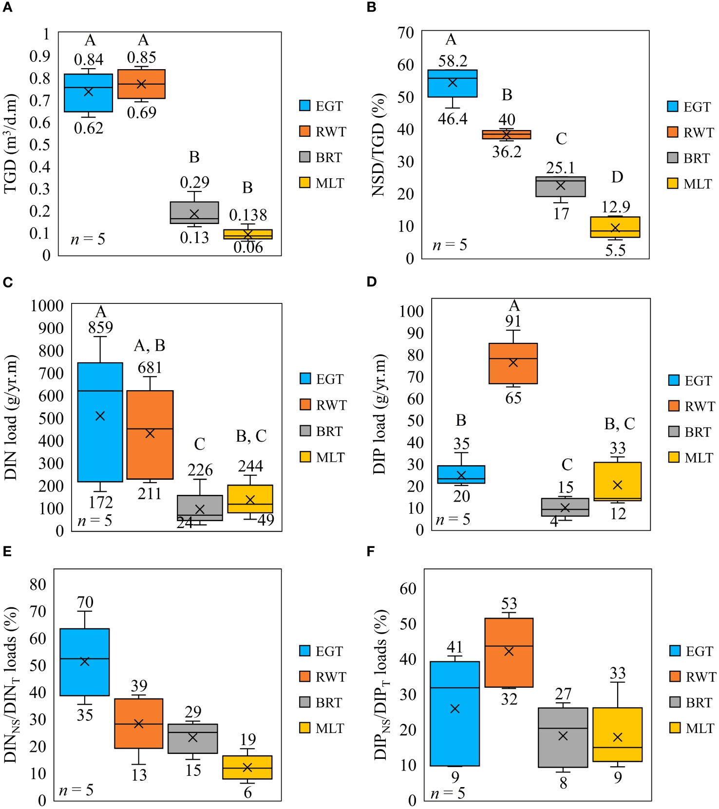
Figure 11 Box and Whisker plots of SEAWAT predicted results and their distributions over the five sampling periods at the four transects including (A) predicted TGD rates through the entire lagoon bed at each transect in cubic meters per day per meter of lagoon shoreline, (B) estimated percentage of TGD from the near-shore zone, (C) estimated annual DIN loads through the entire lagoon beds at each transect, (D) estimated annual DIP loads through the entire lagoon beds at each transect, (E) estimated percentage of DIN load from the near-shore zone, and (F) estimated percentage of DIP load from the near-shore zone. The letters A through D are assigned to tested groups by the one-way ANOVA Tukey test.

The near-shore zone contribution of seepage at the four transects, as compared to the entire transect, is shown in (Figure 11B) as a percentage of NSD/TGD, where NSD stands for near-shore discharge. These percentages ranged from (46.4 to 58.2) %, (36.2 to 40) %, (17 to 25.1) %, and (5.5 to 12.9) % for EGT, RWT, BRT, and MLT, respectively. The near-shore zones contribute significantly different fractions at the four sites according to the one-way ANOVA Tukey’s comparison test conducted at a significance level α = 0.05 (Figure 11B). The higher near-shore contributions at EGT and RWT can be attributed to the fact that they are directly connected to the mainland which is the main supplier of groundwater to the lagoon. The above NSD/TGD percentages are equivalent to NSD rates in m³/d per meter of shoreline ranging from (0.29 to 0.49), (0.25 to 0.34), (0.02 to 0.07), and (0.003 to 0.018) at EGT, RWT, BRT, and MLT, respectively. In a previous investigation, Martin et al. (2007) estimated that discharge rates at the near-shore of EGT ranged from 0.02 to 0.9 m³/day per meter of lagoon shoreline based on two techniques: seepage meters and porewater chloride Cl^- distributions. Our estimated NSD at EGT appears to fall within the range of the seepage rate estimated by Martin et al. (2007). Another study, which also used porewater chloride profiles to solve a one-dimensional advection-diffusion model for seepage velocity, estimated average NSD rates of 0.14, 0.096, and 0.64 m³/day per meter of lagoon shoreline distributed over 17.6 m, 35.7 m, and 67.8 m seepage faces at the near-shore of EGT, RWT, and BRT, respectively (Pain et al., 2021). These previously estimated nearshore seepage rates are within one order of magnitude of our maximum estimated values at the EGT and RWT sites, being slightly smaller, while they are also within one order of magnitude of our maximum estimate at the BRT site, being slightly greater.

The estimated annual DIN and DIP loads at all four transects during each of the events measured during the study period are shown in (Figures 11C, D), respectively. We can observe that the lagoon system receives much higher DIN loads than DIP loads at all study sites during the study period and that makes the lagoon nitrogen-enriched, the result that agrees with the measured nutrient concentrations in the lagoon water (Figure 10F). The estimated annual DIN loads into the lagoon in (g/yr. per meter of lagoon shoreline) at EGT, RWT, BRT, and MLT ranged from (172 to 859), (211 to 681), (24 to 226), and (49 to 244), and averaged annually by 507, 429, 92, and 134, respectively (Figure 11C). This implies that the IRLS receives the highest DIN at the EGT site followed by the RWT site. High temporal variation in the DIN loads is more pronounced at the EGT and RWT sites. Also, the estimated annual DIP loads into the lagoon in (g/yr. per meter of lagoon shoreline) at EGT, RWT, BRT, and MLT ranged from (20 to 35), (65 to 91), (4 to 15), and (12 to 33), and averaged annually by 24, 76, 10, and 20, respectively (Figure 11D). A one-way ANOVA with Tukey’s comparison test revealed no statistically significant difference in DIN loads between the EGT and RWT sites or between the BRT and MLT sites (Figure 11C). No significant difference in the DIN annual loads was also revealed between the RWT and MLT sites. However, similar to what we observed in the comparison of TGD distributions (Figure 11A), The DIN annual loads at the EGT are significantly different from those at the BRT and MLT (Figure 11C). The other observation we obtain from Figures 11C, D is that the DIN and DIP loads are not only spatially variable but are also characterized by large temporal variations over the entire study program. Spatial heterogeneity in nutrient loading was also pronounced for annual DIP loads (Figure 11D), where the RWT showed significantly different DIP loads from all other three sites, whereas no statistical difference was revealed between the EGT and MLT or between the BRT and MLT locations. Overall, these results indicate nutrient loads in the IRLT can differ substantially both between locations and over time.

Nutrients received through the near-shore zones showed significant variations between the four sites as presented in Figures 11E, F for nitrogen (DIN_NS/DIN_T) and phosphorus (DIP_NS/DIP_T) loads percentages, respectively, where the subscript “NS” stands for the nitrogen or phosphorus loads received through the near-shore zone, and the subscript “T” stands for the DIN or DIP loads received through the entire transect. The near-shore zones contribute (35 to 70) %, (13 to 39) %, (15 to 29) %, and (6 to 19) % of the total nitrogen at the EGT, RWT, BRT, and MLT, respectively. Similarly, the near-shore zones contribute (9 to 41) %, (32 to 53) %, (8 to 27) %, and (9 to 33) % of the total phosphorus at the EGT, RWT, BRT, and MLT, respectively. The estimated average annual DINNS loads, expressed in grams per year per meter of shoreline, at the EGT, RWT, BRT, and MLT are 258, 120, 21.25, and 15.97, respectively. Similarly, the estimated average annual DIPNS loads, also expressed in grams per year per meter of shoreline, at the EGT, RWT, BRT, and MLT are 6.34, 32, 1.62, and 3.57, respectively. Previous research conducted by Pain et al. (2021), as mentioned earlier, estimated nearshore DIN loads (calculated as NH₄ + NO₃) at the EGT, RWT, and BRT to be 33.75, 0.62, and 6.04 grams per year per meter of lagoon shoreline, respectively. Pain et al. (2021) also estimated that the nearshore zones of the EGT, RWT, and BRT received DIP loads of 1.71, 0.379, and 1.34 grams per year per meter of shoreline, respectively. Comparing our obtained results for DIN_NS and DIP_NS to the nutrient loads estimated by Pain et al. (2021), it is evident that the two estimates for the EGT and BRT differ by less than an order of magnitude. However, our estimates at the RWT are greater by two orders of magnitude compared to those obtained by Pain et al. (2021).

5.7 Influence of recharge from the Hawthorn formation

The estimated recharge results from the Hawthorn at EGT, RWT, and BRT are shown in Table 4. The numerical models were recalibrated to adjust for the effect of the Hawthorn recharge on the predicted hydraulic head contours, and the resulting predictions for seepages into the IRLS are compared to those predicted by the model under no recharge conditions in Table 4. The inclusion of the estimated recharge through the Hawthorn Formation resulted in a slight increase in the groundwater seepage into the IRLS ranging from a 2.2% difference at EGT to an 8.7% difference at RWT.

TABLE 4

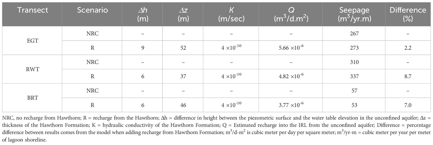
Table 4 Model predicted groundwater seepages into the IRLS under recharge and no recharge conditions from the Hawthorn Formation.

6 Conclusions

Numerical models and a two-year field measurement program were used to assess the amount of terrestrial groundwater discharge and associated nutrient loads into the northern Indian River lagoon at four different transects. Temporal fluctuations in lagoon surface water salinity were observed, with the MLT site being consistently saline, and the EGT, RWT, and BRT sites showing comparable but fluctuating salinity levels. This suggests higher freshwater input at the latter three sites, potentially from sources such as fresh groundwater.

Simulations revealed that saltwater moves downward from the lagoon into the unconfined aquifer, whereas groundwater seepage moves upward from the aquifer to the lagoon. Saltwater intrusion was predicted to occur to a limited extent at transects bordering the ocean. Elevated ammonium concentrations in groundwater were observed at all sites, particularly at MLT, possibly due to in-situ remineralization of sedimental organic matter. Nitrite/nitrate concentrations were highest at EGT, indicating potential anthropogenic contamination, while BRT and RWT showed reduced nitrite/nitrate concentrations, likely due to biogeochemical transformations by mangroves and natural wetlands.

The lagoon surface water exhibited high DIN/DIP molar ratios, suggesting nitrogen enrichment and potential for increased primary production and harmful algal blooms. The highest terrestrial groundwater discharge occurred at EGT and RWT, which are directly connected to the mainland, whereas MLT received the lowest and least variable discharge. The DIN loads were highest at EGT and RWT, reflecting urbanization impacts, with BRT and MLT having lower and less variable DIN loads. The DIP loads were smaller but varied spatially, with RWT showing the highest loads. Near-shore zones significantly contributed to groundwater discharge, nutrient loads, and their ratios, with EGT and RWT exhibiting the highest contributions. The Hawthorn Formation had a limited impact on the estimated nutrient loads.

Data availability statement

The original contributions presented in the study are included in the article/Supplementary Material. Further inquiries can be directed to the corresponding author.

Author contributions

WA: Conceptualization, Data curation, Formal Analysis, Investigation, Methodology, Writing – original draft, Writing – review & editing. KM: Data curation, Formal Analysis, Software, Writing – review & editing. AP: Conceptualization, Funding acquisition, Methodology, Project administration, Writing – original draft. HH: Conceptualization, Investigation, Methodology, Writing – review & editing. AB: Formal Analysis, Software, Writing – original draft.

Funding

The author(s) declare financial support was received for the research, authorship, and/or publication of this article. This work was supported by St. Johns River Water Management District (SJRWMD), Palatka, Florida, through contract #27815.

Acknowledgments

Special thanks to Dr. Charles Jacoby, Supervising Environmental Scientist in the Estuaries Section and Lead Scientist of the Indian River Lagoon Basin at the SJRWMD, for his continuous guidance and encouragement throughout the project.

Conflict of interest

The authors declare that the research was conducted in the absence of any commercial or financial relationships that could be construed as a potential conflict of interest.

Publisher’s note

All claims expressed in this article are solely those of the authors and do not necessarily represent those of their affiliated organizations, or those of the publisher, the editors and the reviewers. Any product that may be evaluated in this article, or claim that may be made by its manufacturer, is not guaranteed or endorsed by the publisher.

Supplementary material

The Supplementary Material for this article can be found online at: https://www.frontiersin.org/articles/10.3389/fmars.2023.1286837/full#supplementary-material

References

Al-Taliby W., Pandit A. (2017). Comparison of solutions of coupled and uncoupled models for the Henry problem. World Environ. Water Resour. Congress 2017, 89–102. doi: 10.1061/9780784480625.010

CrossRef Full Text | Google Scholar

Al-Taliby W., Pandit A. (2023). Estimation of nitrogen and phosphorus fluxes into a Barrier Island lagoon via meteoric groundwater discharge. Sci. Total Environ. 886, 163927. doi: 10.1016/j.scitotenv.2023.163927

PubMed Abstract | CrossRef Full Text | Google Scholar

Al-Taliby W., Pandit A., Heck H. H., Ali N. (2016). Numerical modeling of groundwater flow below an estuary using MODFLOW and SEAWAT—Comparison of results. World Environ. Water Resour. Congress 2016, 265–274. doi: 10.1061/9780784479865.028

CrossRef Full Text | Google Scholar

Anderson M. P., Woessner W. W., Hunt R. J. (2015). Applied Groundwater Modeling: Simulation of Flow and Advective Transport (2^nd Ed.) (San Diego: Academic Press).

Google Scholar

Aquaveo (2011). GMS user manual version 6. Available at: https://media.specialolympics.org/resources/games-and-competition/gms/GMS-6-User-Manual.pdf.

Google Scholar

Bear J. (1979). Hydraulics of groundwater (New York: McGraw-Hill).

Google Scholar

Beck M., Reckhardt A., Amelsberg J., Bartholomä A., Brumsack H.-J., Cypionka H., et al. (2017). The drivers of biogeochemistry in beach ecosystems: A cross-shore transect from the dunes to the low-water line. Mar. Chem. 190, 35–50. doi: 10.1016/j.marchem.2017.01.001

CrossRef Full Text | Google Scholar

Belanger T., Walker R. (1990). Ground water seepage in the Indian River Lagoon, Florida. Tropical Hydrology and Caribbean Water Resources. The International Symposium on Tropical Hydrology and Fourth Caribbean Islands Water Resources Congress. Am. Water Resour. Assoc. Middleburg Va, 367–375.

Google Scholar

Belanger T. V., Montgomery M. T. (1992). Seepage meter errors. Limnol. Oceanogr. 37 (8), 1787–1795. doi: 10.4319/lo.1992.37.8.1787

CrossRef Full Text | Google Scholar

Berber A. (2017). Estimation of Groundwater Loads into a Coastal Estuary Using SEAWAT (Melbourne, FL, USA: Florida Institute of Technology). Available at: http://hdl.handle.net/11141/1411.

Google Scholar

Berndt M. P., Katz B. G., Kingsbury J. A., Crandall C. A. (2014). The quality of our nation’s waters—Water quality in the upper Floridan aquifer and overlying surficial aquifers, Southeastern United States 1993–2010. U.S. Geol. Survey Circ. 1355, 72. (Reston, VA: U.S. Geological Survey) doi: 10.3133/cir1355

CrossRef Full Text | Google Scholar

Burnett W. C., Aggarwal P. K., Aureli A., Bokuniewicz H., Cable J. E., Charette M. A., et al. (2006). Quantifying submarine groundwater discharge in the coastal zone via multiple methods. Sci. Total Environ. 367 (2–3), 498–543. doi: 10.1016/j.scitotenv.2006.05.009

PubMed Abstract | CrossRef Full Text | Google Scholar

Burnett W. C., Kim G., Lane-Smith D. (2001). A continuous monitor for assessment of 222Rn in the coastal ocean. J. Radioanal. Nucl. Chem. 249 (1), 167–172. doi: 10.1023/A:1013217821419

CrossRef Full Text | Google Scholar

Bush P. W., Johnston R. H. (1988). Ground-water Hydraulics, Regional Flow, and Groundwater Development of the Floridan Aquifer System in Florida and Parts of GEORGIA, South Carolina, and 562 Alabama. U.S. Geological Survey Professional Paper 1403–C. 80 p. (Washington, D.C: U.S. Government Printing Office).

Google Scholar

Cable J. E., Bugna G. C., Burnett W. C., Chanton J. P. (1996). Application of ²²² Rn and CH ₄ for assessment of groundwater discharge to the coastal ocean. Limnol. Oceanogr. 41 (6), 1347–1353. doi: 10.4319/lo.1996.41.6.1347

CrossRef Full Text | Google Scholar

Cable J. E., Corbett D. R., Walsh M. M. (2002). Phosphate uptake in coastal limestone aquifers: A fresh look at wastewater management. Limnol. Oceanogr. Bull. 11 (2), 29–32. doi: 10.1002/lob.200211229

CrossRef Full Text | Google Scholar

Cabral A., Sugimoto R., Taniguchi M., Tait D., Nakajima T., Honda H., et al. (2023). Fresh and saline submarine groundwater discharge as sources of carbon and nutrients to the Japan Sea. Mar. Chem. 249, 104209. doi: 10.1016/j.marchem.2023.104209

CrossRef Full Text | Google Scholar

Carruthers T. J. B., van Tussenbroek B. I., Dennison W. C. (2005). Influence of submarine springs and wastewater on nutrient dynamics of Caribbean seagrass meadows. Estuar. Coast. Shelf Sci. 64 (2–3), 191–199. doi: 10.1016/j.ecss.2005.01.015

CrossRef Full Text | Google Scholar

Chanyotha S., Kranrod C., Burnett W. C., Lane-Smith D., Simko J. (2014). Prospecting for groundwater discharge in the canals of Bangkok via natural radon and thoron. J. Hydrol. 519, 1485–1492. doi: 10.1016/j.jhydrol.2014.09.014

CrossRef Full Text | Google Scholar

Charette M. A., Buesseler K. O. (2004). Submarine groundwater discharge of nutrients and copper to an urban subestuary of Chesapeake Bay (Elizabeth River). Limnol. Oceanogr. 49 (2), 376–385. doi: 10.4319/lo.2004.49.2.0376

CrossRef Full Text | Google Scholar

Charette M. A., Sholkovitz E. R. (2002). Oxidative precipitation of groundwater-derived ferrous iron in the subterranean estuary of a coastal bay. Geophys. Res. Lett. 29 (10), 85-1-85–4. doi: 10.1029/2001GL014512

CrossRef Full Text | Google Scholar

Corbett D. R., Cable J. E. (2003). Seepage meters and advective transport in coastal environments: Comments on “Seepage meters and Bernoulli’s revenge” by E.A. Shinn, C. D. Reich and T. D. Hickey. 2002. Estuaries 25:126–132. Estuaries 26 (5), 1383–1387. doi: 10.1007/BF02803639

CrossRef Full Text | Google Scholar

Dawes C. J., Hanisak D., Kenworthy J. W. (1995). Seagrass biodiversity in the Indian river lagoon. Bull. Mar. Sci. 57 (1), 59–66.

Google Scholar

Decleyre H., Heylen K., Van Colen C., Willems A. (2015). Dissimilatory nitrogen reduction in intertidal sediments of a temperate estuary: small scale heterogeneity and novel nitrate-to-ammonium reducers. Front. Microbiol. 6. doi: 10.3389/fmicb.2015.01124

PubMed Abstract | CrossRef Full Text | Google Scholar

Dimova N. T., Swarzenski P. W., Dulaiova H., Glenn C. R. (2012). Utilizing multichannel electrical resistivity methods to examine the dynamics of the fresh water-seawater interface in two Hawaiian groundwater systems. J. Geophys. Res.: Oceans 117 (C2). doi: 10.1029/2011JC007509. n/a-n/a.

CrossRef Full Text | Google Scholar

Doherty J. (2010). PEST, Model-independent parameter estimation—User manual 5th Edition (Brisbane, Australia: Watermark Numerical Computing).

Google Scholar

Environmental Simulations Inc. (2011) Guide to using Groundwater Vistas. Available at: https://www.groundwatermodels.com/Groundwater_Vistas.php.

Google Scholar

Erler D. V., Santos I. R., Zhang Y., Tait D. R., Befus K. M., Hidden A., et al. (2014). Nitrogen transformations within a tropical subterranean estuary. Mar. Chem. 164, 38–47. doi: 10.1016/j.marchem.2014.05.008

CrossRef Full Text | Google Scholar

Evans T. B., White S. M., Wilson A. M. (2020). Coastal groundwater flow at the nearshore and embayment scales: A field and modeling study. Water Resour. Res. 56 (10). doi: 10.1029/2019WR026445

CrossRef Full Text | Google Scholar

Gilmore R. G., Hastings P. A., Herrema D. J. (1983). Ichthyofaunal additions to the Indian River Lagoon and adjacent waters, east-central Florida. Florida Scientist 46 (1), 22–30.

Google Scholar

Goodarzi M. S., Amiri B. J., Azarneyvand H., Khazaee M., Mahdianzadeh N. (2020). Assessing the performance of a hydrological tank model at various spatial scales. J. Water Manage. Model. 29. doi: 10.14796/JWMM.C472

CrossRef Full Text | Google Scholar

Harbaugh B. A. W., Banta E. R., Hill M. C., Mcdonald M. G. (2000). MODFLOW-2000, The U.S. Geological Survey modular graound-water model —User guide to modularization concepts and the ground-water flow process. Open-File Report 00-92, 121p. (Reston, VA: U.S. Geological Survey) doi: 10.3133/ofr200092

CrossRef Full Text | Google Scholar

Howarth R. W. (2008). Coastal nitrogen pollution: A review of sources and trends globally and regionally. Harmful Algae 8 (1), 14–20. doi: 10.1016/j.hal.2008.08.015

CrossRef Full Text | Google Scholar

Hu C., Muller-Karger F. E., Swarzenski P. W. (2006). Hurricanes, submarine groundwater discharge, and Florida’s red tides. Geophys. Res. Lett. 33 (11), 2005GL025449. doi: 10.1029/2005GL025449

CrossRef Full Text | Google Scholar

Johnson A. G., Glenn C. R., Burnett W. C., Peterson R. N., Lucey P. G. (2008). Aerial infrared imaging reveals large nutrient-rich groundwater inputs to the ocean. Geophys. Res. Lett. 35 (15), L15606. doi: 10.1029/2008GL034574

CrossRef Full Text | Google Scholar

Kaleris V., Lagas G., Marczinek S., Piotrowski J. A. (2002). Modelling submarine groundwater discharge: an example from the western Baltic Sea. J. Hydrol. 265 (1–4), 76–99. doi: 10.1016/S0022-1694(02)00093-8

CrossRef Full Text | Google Scholar

Knee K. L., Paytan A. (2011). “Submarine groundwater discharge,” in Treatise on Estuarine and Coastal Science (Elsevier), 205–233. doi: 10.1016/B978-0-12-374711-2.00410-1

CrossRef Full Text | Google Scholar

Kwon H. K., Kang H., Oh Y. H., Park S. R., Kim G. (2017). Green tide development associated with submarine groundwater discharge in a coastal harbor, Jeju, Korea. Sci. Rep. 7 (1), 6325. doi: 10.1038/s41598-017-06711-0

PubMed Abstract | CrossRef Full Text | Google Scholar

Langevin C. D. (2003). Simulation of submarine ground water discharge to a marine estuary: Biscayne Bay, Florida. Ground Water 41 (6), 758–771. doi: 10.1111/j.1745-6584.2003.tb02417.x

PubMed Abstract | CrossRef Full Text | Google Scholar

Langevin C. D., Thorne D. T. Jr., Dausman A. M., Sukop M. C., Guo W. (2008). SEAWAT Version 4: A Computer Program for Simulation of Multi-Species Solute and Heat Transport. Techniques and Methods Book 6, Chapter A22. (Reston, VA: U.S. Geological Survey) doi: 10.3133/tm6A22

CrossRef Full Text | Google Scholar

Lee Y.-W., Hwang D.-W., Kim G., Lee W.-C., Oh H.-T. (2009). Nutrient inputs from submarine groundwater discharge (SGD) in Masan Bay, an embayment surrounded by heavily industrialized cities, Korea. Sci. Total Environ. 407 (9), 3181–3188. doi: 10.1016/j.scitotenv.2008.04.013

PubMed Abstract | CrossRef Full Text | Google Scholar

Liefer J. D., MacIntyre H. L., Su N., Burnett W. C. (2014). Seasonal alternation between groundwater discharge and benthic coupling as nutrient sources in a shallow coastal lagoon. Estuar. Coasts 37 (4), 925–940. doi: 10.1007/s12237-013-9739-4

CrossRef Full Text | Google Scholar

Lino Y., Pranjal K., Priyansh S., Jagath C., Udayashankar H. N., Suresh Babu D. S., et al. (2023). Submarine Groundwater Discharge (SGD): Impacts, challenges, limitations, and management recommendations. Groundwater Sustain. Dev. 21, 100903. doi: 10.1016/j.gsd.2023.100903

CrossRef Full Text | Google Scholar

Liu J., Du J., Wu Y., Liu S. (2018). Nutrient input through submarine groundwater discharge in two major Chinese estuaries: the Pearl River Estuary and the Changjiang River Estuary. Estuar. Coast. Shelf Sci. 203, 17–28. doi: 10.1016/j.ecss.2018.02.005

CrossRef Full Text | Google Scholar

Luijendijk E., Gleeson T., Moosdorf N. (2020). Fresh groundwater discharge insignificant for the world’s oceans but important for coastal ecosystems. Nat. Commun. 11 (1), 1260. doi: 10.1038/s41467-020-15064-8

PubMed Abstract | CrossRef Full Text | Google Scholar

Martin J. B., Cable J. E., Smith C., Roy M., Cherrier J. (2007). Magnitudes of submarine groundwater discharge from marine and terrestrial sources: Indian River Lagoon, Florida. Water Resour. Res. 43 (5), 5440. doi: 10.1029/2006WR005266

CrossRef Full Text | Google Scholar

McGurk B., Presley P. F. (2002). Simulation of the Effects of Groundwater Withdrawals on the Floridan Aquifer System in East-Central Florida: Model Expansion and Revision (Palatka, FL: St. Johns River Water Management District Technical Publication, (SJ2002-5)).

Google Scholar

Michael H. A., Lubetsky J. S., Harvey C. F. (2003). Characterizing submarine groundwater discharge: A seepage meter study in Waquoit Bay, Massachusetts. Geophys. Res. Lett. 30 (6). doi: 10.1029/2002GL016000

CrossRef Full Text | Google Scholar

Microsoft Corporation. (2016). Microsoft Excel. Available at: https://office.microsoft.com/excel.

Google Scholar

Miller J. A. (1986). Hydrogeologic framework of the Floridan aquifer system in Florida and in parts of Georgia, South Carolina, and Alabama. U. S. Geological Survey Professional Paper 1403 B. (Reston, VA: U.S. Geological Survey) doi: 10.3133/pp1403B

CrossRef Full Text | Google Scholar

Montiel D., Lamore A., Stewart J., Dimova N. (2019). Is submarine groundwater discharge (SGD) important for the historical fish kills and harmful algal bloom events of mobile bay? Estuar. Coasts 42 (2), 470–493. doi: 10.1007/s12237-018-0485-5

CrossRef Full Text | Google Scholar

Moore W. S. (1996). Large groundwater inputs to coastal waters revealed by 226Ra enrichments. Nature 380 (6575), 612–614. doi: 10.1038/380612a0

CrossRef Full Text | Google Scholar

Moore W. S. (1999). The subterranean estuary: a reaction zone of ground water and sea water. Mar. Chem. 65 (1–2), 111–125. doi: 10.1016/S0304-4203(99)00014-6

CrossRef Full Text | Google Scholar

Moore W. S. (2010). The effect of submarine groundwater discharge on the ocean. Annu. Rev. Mar. Sci. 2 (1), 59–88. doi: 10.1146/annurev-marine-120308-081019

CrossRef Full Text | Google Scholar

Moore W. S., Church T. M. (1996). Submarine groundwater discharge. Nature 382 (6587), 122–122. doi: 10.1038/382122a0

CrossRef Full Text | Google Scholar

Morris L. J., Hall L. M., Jacoby C. A., Chamberlain R. H., Hanisak M. D., Miller J. D., et al. (2022). Seagrass in a changing estuary, the Indian River Lagoon, Florida, United States. Front. Mar. Sci. 8. doi: 10.3389/fmars.2021.789818

CrossRef Full Text | Google Scholar

Nash J. E., Sutcliffe J. V. (1970). River flow forecasting through conceptual models part I — A discussion of principles. J. Hydrol. 10 (3), 282–290. doi: 10.1016/0022-1694(70)90255-6

CrossRef Full Text | Google Scholar

National Climatic Data Center (2001). Monthly station normals of temperature, precipitation, and heating and cooling degree days 1971–2000, Climatography of the United States No. 81. National Oceanic and Atmospheric Administration.

Google Scholar

Oberdorfer J. A. (2003). Hydrogeologic modeling of submarine groundwater discharge: comparison to other quantitative methods. Biogeochemistry 66 (1/2), 159–169. doi: 10.1023/B:BIOG.0000006096.94630.54

CrossRef Full Text | Google Scholar

Pain A. J., Martin J. B., Young C. R. (2021). Biogeochemical and hydrological drivers of heterogeneous nutrient exports from subterranean estuaries. Front. Mar. Sci. 8. doi: 10.3389/FMARS.2021.699916/BIBTEX

CrossRef Full Text | Google Scholar

Pandit A., El-Khazen C. (1990). Groundwater seepage into the Indian River Lagoon at Port St. Lucie. Florida Scientist 53 (3), 169–179.

Google Scholar

Pavlidou A., Papadopoulos V. P., Hatzianestis I., Simboura N., Patiris D., Tsabaris C. (2014). Chemical inputs from a karstic submarine groundwater discharge (SGD) into an oligotrophic Mediterranean coastal area. Sci. Total Environ. 488–489, 1–13. doi: 10.1016/j.scitotenv.2014.04.056

PubMed Abstract | CrossRef Full Text | Google Scholar

Phlips E. J., Badylak S., Grosskopf T. (2002). Factors affecting the abundance of phytoplankton in a restricted subtropical lagoon, the Indian River Lagoon, Florida, USA. Estuar. Coast. Shelf Sci. 55 (3), 385–402. doi: 10.1006/ECSS.2001.0912

CrossRef Full Text | Google Scholar

Phlips E. J., Badylak S., Youn S., Kelley K. (2004). The occurrence of potentially toxic dinoflagellates and diatoms in a subtropical lagoon, the Indian River Lagoon, Florida, USA. Harmful Algae 3 (1), 39–49. doi: 10.1016/J.HAL.2003.08.003

CrossRef Full Text | Google Scholar

Ptacnik R., Andersen T., Tamminen T. (2010). Performance of the redfield ratio and a family of nutrient limitation indicators as thresholds for phytoplankton N vs. P limitation. Ecosystems 13 (8), 1201–1214. doi: 10.1007/s10021-010-9380-z

CrossRef Full Text | Google Scholar

Reckhardt A., Beck M., Greskowiak J., Schnetger B., Böttcher M. E., Gehre M., et al. (2017). Cycling of redox-sensitive elements in a sandy subterranean estuary of the southern North Sea. Mar. Chem. 188, 6–17. doi: 10.1016/j.marchem.2016.11.003

CrossRef Full Text | Google Scholar

Redfield A. C. (1958). The biological control of chemical factors in the environment. Am. Scientist 46 (3), 230A–2221.

Google Scholar

Russoniello C. J., Heiss J. W., Michael H. A. (2018). Variability in benthic exchange rate, depth, and residence time beneath a shallow coastal estuary. J. Geophys. Res.: Oceans 123 (3), 1860–1876. doi: 10.1002/2017JC013568

CrossRef Full Text | Google Scholar

Santos I. R., Burnett W. C., Chanton J., Dimova N., Peterson R. N. (2009). Land or ocean?: Assessing the driving forces of submarine groundwater discharge at a coastal site in the Gulf of Mexico. J. Geophys. Res. 114 (C4), C04012. doi: 10.1029/2008JC005038

CrossRef Full Text | Google Scholar

Santos I. R., Chen X., Lecher A. L., Sawyer A. H., Moosdorf N., Rodellas V., et al. (2021). Submarine groundwater discharge impacts on coastal nutrient biogeochemistry. Nat. Rev. Earth Environ. 2 (5), 307–323. doi: 10.1038/s43017-021-00152-0

CrossRef Full Text | Google Scholar

Sawyer A. H., David C. H., Famiglietti J. S. (2016). Continental patterns of submarine groundwater discharge reveal coastal vulnerabilities. Science 353 (6300), 705–707. doi: 10.1126/science.aag1058

PubMed Abstract | CrossRef Full Text | Google Scholar

Schiffer D. M. (1998). Hydrology of Central Florida Lakes - A Primer . U.S. Geological Survey circular 1137. (Reston, VA: U.S. Geological Survey). doi: 10.3133/cir1137

CrossRef Full Text | Google Scholar

Scott T. M. (1988). The Lithostratigraphy of the Hawthorn Group (Miocene) of Florida (Tallahassee: Fl. Geol. Surv.). Bulletin No. 59. doi: 10.35256/B59

CrossRef Full Text | Google Scholar

Sigua G. C., Tweedale W. A. (2003). Watershed scale assessment of nitrogen and phosphorus loadings in the Indian River Lagoon basin, Florida. J. Environ. Manage. 67 (4), 363–372. doi: 10.1016/S0301-4797(02)00220-7

PubMed Abstract | CrossRef Full Text | Google Scholar

Smith L., Zawadzki W. (2003). hydrogeologic model of submarine groundwater discharge: Florida intercomparison experiment. Biogeochemistry 66 (1/2), 95–110. doi: 10.1023/B:BIOG.0000006108.80520.c9

CrossRef Full Text | Google Scholar

Steward J. S., Virnstein R. W., Morris L. J., Lowe E. F. (2005). Setting seagrass depth, coverage, and light targets for the Indian River Lagoon system, Florida. Estuaries 28 (6), 923–935. doi: 10.1007/BF02696020

CrossRef Full Text | Google Scholar

Stieglitz T., Rapaglia J., Bokuniewicz H. (2008). Estimation of submarine groundwater discharge from bulk ground electrical conductivity measurements. J. Geophys. Res. 113 (C8), C08007. doi: 10.1029/2007JC004499

CrossRef Full Text | Google Scholar

St Johns River Water Management District (2012) Indian River Lagoon 2011 Superbloom: Plan of Investigation. Available at: https://www.sjrwmd.com/documents/technical-reports/technical-publications/.

Google Scholar

Swarzenski P. W., Burnett W. C., Greenwood W. J., Herut B., Peterson R., Dimova N., et al. (2006). Combined time-series resistivity and geochemical tracer techniques to examine submarine groundwater discharge at Dor Beach, Israel. Geophys. Res. Lett. 33 (24). doi: 10.1029/2006GL028282

PubMed Abstract | CrossRef Full Text | Google Scholar

Szymczycha B., Kłostowska Ż., Lengier M., Dzierzbicka-Głowacka L. (2020). Significance of nutrient fluxes via submarine groundwater discharge in the Bay of Puck, southern Baltic Sea. Oceanologia 62 (2), 117–125. doi: 10.1016/j.oceano.2019.12.004

CrossRef Full Text | Google Scholar

Tamborski J. J., Rogers A. D., Bokuniewicz H. J., Cochran J. K., Young C. R. (2015). Identification and quantification of diffuse fresh submarine groundwater discharge via airborne thermal infrared remote sensing. Remote Sens. Environ. 171, 202–217. doi: 10.1016/j.rse.2015.10.010

CrossRef Full Text | Google Scholar

Taniguchi M., Burnett W. C., Cable J. E., Turner J. V. (2002). Investigation of submarine groundwater discharge. Hydrol. Processes 16 (11), 2115–2129. doi: 10.1002/hyp.1145

CrossRef Full Text | Google Scholar

Taniguchi M., Burnett W. C., Dulaiova H., Kontar E. A., Povinec P. P., Moore W. S. (2006). Submarine groundwater discharge measured by seepage meters in sicilian coastal waters. Continental Shelf Res. 26 (7), 835–842. doi: 10.1016/j.csr.2005.12.002

CrossRef Full Text | Google Scholar

Taniguchi M., Dulai H., Burnett K. M., Santos I. R., Sugimoto R., Stieglitz T., et al. (2019). Submarine groundwater discharge: updates on its measurement techniques, geophysical drivers, magnitudes, and effects. Front. Environ. Sci. 7. doi: 10.3389/fenvs.2019.00141

CrossRef Full Text | Google Scholar

Uma K. O., Egboka B. C. E., Onuoha K. M. (1989). New statistical grain-size method for evaluating the hydraulic conductivity of sandy aquifers. J. Hydrol. 108, 343–366. doi: 10.1016/0022-1694(89)90293-X

CrossRef Full Text | Google Scholar

Unnikrishnan P., Srinivas R., Ramasamy M., Suresh Babu D. S. (2021). Computation of submarine groundwater discharge from geomorphologically different coastal catchments of SW India using numerical modeling. Regional Stud. Mar. Sci. 47, 101963. doi: 10.1016/j.rsma.2021.101963

CrossRef Full Text | Google Scholar

Waska H., Kim G. (2010). Differences in microphytobenthos and macrofaunal abundances associated with groundwater discharge in the intertidal zone. Mar. Ecol. Prog. Ser. 407, 159–172. doi: 10.3354/meps08568

CrossRef Full Text | Google Scholar

Wilson A. M. (2005). Fresh and saline groundwater discharge to the ocean: A regional perspective. Water Resour. Res. 41 (2). doi: 10.1029/2004WR003399

PubMed Abstract | CrossRef Full Text | Google Scholar

Wilson J., Rocha C. (2012). Regional scale assessment of Submarine Groundwater Discharge in Ireland combining medium resolution satellite imagery and geochemical tracing techniques. Remote Sens. Environ. 119, 21–34. doi: 10.1016/j.rse.2011.11.018

CrossRef Full Text | Google Scholar

Xiao H., Wang D., Medeiros S. C., Bilskie M. V., Hagen S. C., Hall C. R. (2019). Exploration of the effects of storm surge on the extent of saltwater intrusion into the surficial aquifer in coastal east-central Florida (USA). Sci. Total Environ. 648, 1002–1017. doi: 10.1016/j.scitotenv.2018.08.199

PubMed Abstract | CrossRef Full Text | Google Scholar

Zheng C., Wang P. (1999). MT3DMS-A Modular Three-dimensional Multispecies Transport Model for Simulation of Advection, Dispersion, and Chemical Reaction of Contaminants in Ground-water Systems: Documentation and User’s Guide.. U.S. Army Corps of Engineers, Contract Report SERDP-99-1. Washington, D.C.

Google Scholar