PHI-SMFE: spatial multi-scale feature extract neural network based on physical heterogeneous interaction for solving passive scalar advection in a 2-D unsteady flow

Fluid dynamic calculations play a crucial role in understanding marine biochemical dynamic processes, impacting the behavior, interactions, and distribution of biochemical components in aquatic environments. The numerical simulation of fluid dynamics is a challenging task, particularly in real-world scenarios where fluid motion is highly complex. Traditional numerical simulation methods enhance accuracy by increasing the resolution of the computational grid. However, this approach comes with a higher computational demand. Recent advancements have introduced an alternative by leveraging deep learning techniques for fluid dynamic simulations. These methods utilize discretized learned coefficients to achieve high-precision solutions on low-resolution grids, effectively reducing the computational burden while maintaining accuracy. Yet, existing fluid numerical simulation methods based on deep learning are limited by their single-scale analysis of spatially correlated physical fields, which fails to capture the diverse scale characteristics inherent in flow fields governed by complex laws in different physical space. Additionally, these models lack an effective approach to enhance correlation interactions among dynamic fields within the same system. To tackle these challenges, we propose the Spatial Multi-Scale Feature Extract Neural Network based on Physical Heterogeneous Interaction (PHI-SMFE). The PHI module is designed to extract heterogeneity and interaction information from diverse dynamic fields, while the SMFE module focuses on capturing multi-scale features in fluid dynamic fields. We utilize channel-biased convolution to implement a separation strategy, reducing the processing of redundant feature information. Furthermore, the traditional solution module based on the finite volume method is integrated into the network to facilitate the numerical solution of the discretized dynamic field in subsequent time steps. Comparative analysis with the current state-of-the-art model reveals that our proposed method offers a 41% increase in simulation accuracy and a 12.7% decrease in inference time during the iterative evolution of unsteady flow. These results underscore the superior performance of our model in terms of both simulation accuracy and computational speedup, establishing it as a state-of-the-art solution.

1 Introduction

Fluid dynamics calculations play a crucial role in marine biochemical domains, including air pollution (Wei et al., 2020), climate change (Benmoshe et al., 2012), engine engineering design (Arcoumanis and Whitelaw, 1987), and physical science (Tang and Chan, 2005). By comprehending and manipulating fluid flow, these calculations facilitate the anticipation of nutrient dispersion, oxygen diffusion, solute conveyance, particle migration, and other phenomena.

Traditional approaches for fluid numerical simulations involve employing grid discretization of the continuity equations and physical fields. Stuart (2009) proposed a finite-difference based mesh technique to solve the governing equations of fluid motion. This approach has the advantage of considering the intricate characteristics of fluid motion, including the fluid structure and energy conversion processes. Spalart and Allmaras (1992) introduced a gridded fluid numerical simulation technique based on the finite volume method. This method utilizes a single transport approach incorporating eddy viscosity to model fluid effects, leading to enhanced predictive capability and accuracy in complex engineering scenarios. However, the traditional gridding method faces a drawback of high computational complexity as the grid resolution increases. This limitation poses challenges when applying the method to simulate complex fluid characteristics with hierarchical structures in practical scenarios.

High-precision numerical simulation acceleration methods based on traditional gridding models have been developed to address the aforementioned challenges. These methods primarily focus on improving the grid generation process, resulting in accelerated simulations without compromising the accuracy of the results. Research in this field has focused on two main aspects. Firstly, there is a growing interest in achieving high-precision simulation of complex fluid motion. One prominent method in this regard is Large Eddy Simulation (LES) (Lesieur and Metais, 1996), which has found widespread applications in various engineering domains including internal combustion engines (Malé et al., 2019), turbomachinery (Arroyo et al., 2019), and gas turbine engine design (Esclapez et al., 2017). On the other hand, parallel efforts have been made to address the challenge of computational complexity in high-precision simulation. One such method is Reynolds-averaged Navier-Stokes (RANS) (Alfonsi, 2009), which is a highly efficient fluid numerical simulation technique. The fundamental concept of this method involves averaging the Navier-Stokes equations, resulting in a set of Reynolds-averaged equations that are computationally more tractable to solve. In essence, the RANS method allows for the prediction of the average behavior of fluid without explicitly resolving the fluid fluctuations at each point, thus reducing the computational cost of the simulation. However, as the RANS method averages the fluid field over time, it loses the detailed information about the unstable structures in the flow, making it unsuitable for simulating unstable and complex flows. Building upon the RANS method, Shur et al. (1999) introduced detached eddy simulation (DES). DES addresses the limitations of RANS and LES methods in simulating complex fluid by employing high-resolution grids near the wall region and low-resolution grids in the outer region. However, such traditional numerical simulation methods have certain limitations. Firstly, when dealing with high Reynolds number flows, these methods still incur high computational costs, demanding significant computing resources and time. Consequently, they may lack real-time capability in simulation prediction tasks and the ability to make timely engineering decisions. Secondly, the extent to which traditional numerical simulation methods truly enable a deep understanding of fluid behavior and fluid systems remains a subject of investigation.

Based on the aforementioned research, traditional methods have faced a trade-off between simulation accuracy and computational performance, which remains a bottleneck in current fluid numerical simulation. In recent years, there has been an emerging trend in combining traditional numerical simulation methods with machine learning techniques. Deep learning-based numerical simulation methods have demonstrated potential in achieving a balance between accuracy and computational efficiency. Kochkov et al. (2021) applied a deep learning-based acceleration method to numerical simulation of high-resolution flow fields. Their approach achieved a significant computational acceleration of 40-80 times compared to traditional benchmark solvers, while maintaining comparable accuracy. Zhuang et al. (2021) applied the aforementioned method to solve the advection equation in two-dimensional flow. They specifically focused on analyzing small-scale features in complex flow and conducting numerical simulation of turbulent flow fields at low resolution. Notably, their method achieved comparable accuracy to a baseline high-order solver, even when the baseline mesh was four times coarser, resulting in a computational speedup of approximately five times.

However, the previously mentioned numerical simulation method based on deep learning relies on a singlescale convolutional neural network to analyze the physical field with spatial-temporal correlation. This approach has limitations in effectively capturing the multi-scale flow field in space, especially when dealing with complex motion patterns of vortex clusters at different scales. Additionally, the spatial discretization of the velocity field can impact the evolution of the concentration field over time. Furthermore, the convolution filtering fusion strategy may not adequately facilitate the partial interaction among different physical fields. These challenges can result in the model’s limited ability to fully learn the differential coefficients that better match the actual behavior, consequently leading to a reduction in simulation accuracy. To address these challenges, we have introduced a novel approach that incorporates a spatial multi-scale feature extraction module to enhance the accuracy of numerical simulation by capturing the intricate characteristics of turbulent eddies across different scales within the flow field. Additionally, we have devised a physical heterogeneity fusion module to augment the heterogeneity of the velocity field and concentration field in the spatial domain while establishing global correlations between them. Moreover, to optimize computational efficiency, we have improved upon the traditional convolution operator by implementing a separation strategy that selectively retains intermediate feature information across specific channels, thereby reducing redundant computational processing.

In summary, our contributions can be categorized as follows.

● Our first contribution lies in addressing the impact of the divergence-free velocity field on the scalar concentration field by taking into account the advective form of the concentration field. To enhance the representation of the velocity field and the concentration field characteristics, we propose a pre-fusion module. This module enables us to capture the heterogeneity and nonlinear interaction information of the physical field in advance, leading to an improved understanding of the nature of the velocity field and the concentration field.

● We have developed a spatial multi-scale neural network with ASPP as the backbone, which enables the learning of eddy characteristics and motion patterns at different scales from the fluid dynamic field, leading to enhanced accuracy in numerical simulations. Furthermore, the inclusion of deredundant sidechannel convolutions within the backbone network reduces the need for extensive feature processing, resulting in accelerated numerical computations.

● We conducted comprehensive experiments, including comparisons with the baseline model and ablation studies, using a random velocity field dataset. Additionally, we performed experiments using constant velocity fields and deformed flow velocity fields to assess the model’s performance under different flow conditions. Our method demonstrates significant improvements compared to the current baseline model, achieving a 41% higher simulation accuracy and a 12.7% reduction in inference time during the iterative evolution of the unsteady flow field. These results highlight that our proposed model achieves state-of-the-art performance in terms of both simulation accuracy and computation speedup.

This paper is developed as follows: chapter 2 provides a comprehensive overview of recent advancements that have significantly contributed to fluid numerical simulation. In chapter 3, we propose a novel model called Spatial multi-scale feature extract neural network based on physical heterogeneous interaction to enhance the performance of numerical simulation in passive scalar advection. Our model leverages the Atrous Spatial Pyramid Pooling (ASPP) as the backbone network to capture spatial scale information from the two-dimensional discretized dynamic fields. Prior to the backbone, a feature fusion module is employed to extract the heterogeneity and interaction information among different dynamic fields. Notably, within the backbone, the channel-side convolution employs a separation strategy to minimize the processing of redundant feature information. Subsequently, chapter 4 is dedicated to conducting comparative experiments aimed at validating the overall model’s superior performance in classic test cases. Additionally, we conduct ablation experiments within this chapter to assess the performance impact of each sub-module within the network model on the system as a whole. Finally, in chapter 5, we summarize the proposed methods and their contributions. We also outline potential directions for further improvement by analyzing the experimental results.

2 Related work

2.1 Traditional fluid numerical calculation methods

The purpose of numerical simulation in fluid dynamics is to facilitate the study and comprehension of fluid behavior and the underlying principles governing fluid flow in various scenarios. During the early stages of fluid dynamics numerical simulation, conventional methods were employed, which involved discretizing the fluid domain into grid nodes to facilitate numerical calculations. These traditional methods encompassed fundamental techniques such as the finite difference method (Simos and Williams, 1997), finite volume method (Jameson et al., 1981), and finite element method (Bassi and Rebay, 1997). The classical methods mentioned discretize the computational domain of the original nonlinear partial differential equations, which consist of continuity equations, diffusion equations, and other relevant equations. This discretization process involves dividing the domain into grid nodes and formulating the equations in a discretized form. By doing so, the continuous equations are transformed into a set of discrete equations that can be solved numerically. In addition to the aforementioned methods, there are other numerical techniques utilized for fluid calculations, such as spectral methods and pseudospectral methods. Spectral methods employ fourier series to approximate the solutions of partial differential equations, aiming to achieve high accuracy by capturing the spectral content of the solution (Feit et al., 1982). However, these methods directly evaluate the nonlinear terms of the partial differential equations in physical space, which can lead to computationally expensive calculations and potential numerical instability issues. Subsequently, pseudospectral methods (Garg et al., 2010), which combine the advantages of spectral methods and finitedifference techniques, emerged as an alternative approach. Pseudospectral methods involve computing the nonlinear terms in fourier space, where they can be efficiently evaluated using fast fourier transforms, and then transforming them back to physical space using inverse fourier transforms (Orszag, 1974). Orszag (1972) conducted a comparative study of these methods in various model problems and demonstrated the effectiveness and stability of pseudospectral methods. Patera (1984) further extended the application of pseudospectral methods by combining them with the finite element method to solve the one-dimensional advection-diffusion equation, which proved useful in simulating laminar separation flow in channel expansion. Krastev and Schäfer (2005) proposed a pseudospectral solver with multigrid techniques for the numerical prediction of incompressible nonisothermal flow. These developments showcased the potential of pseudospectral methods in achieving accurate and efficient solutions for fluid dynamics problems.

2.2 Acceleration method for traditional fluid numerical simulation

Traditional fluid numerical simulation methods often face challenges when dealing with fluids exhibiting complex motion characteristics. These methods can be computationally demanding and time-consuming, limiting their efficiency and practicality in real-world applications. To address these issues, the development of fluid numerical simulation acceleration methods has gained attention. The primary objective of these methods is to reduce the computational burden while accurately capturing the intricate flow features at small scales. By achieving faster simulations of fluid fields, these acceleration methods aim to enhance the applicability of numerical simulation in engineering practice. Traditional methods for accelerating fluid numerical simulations include the multi-grid method (Alcouffe et al., 1981) and the adaptive grid method (Hiptmair, 1998). The multi-grid method is a convergence acceleration technique that combines iterative methods with coarse grid corrections. It involves generating grids at different scales to iteratively solve the discretized partial differential equations. The main advantage of this method is that it speeds up the numerical solution process through iterative computations, while the use of grids at different scales helps eliminate error components of varying wavelengths. Jameson (1993) successfully applied the multi-grid method to accelerate the computation of transonic potential flow. His proposed multi-grid alternating direction method demonstrated high efficiency and reliability in practical experiments. Ghia et al. (1982) introduced the coupled strong implicit multi-grid method (CSI-MG) for solving fine-grid incompressible flow with high Reynolds numbers. This method yielded solutions for fluid motion scenarios with a grid size of 257*257 and a Reynolds number of 10000. However, it should be noted that this method faces challenges in generating coarse meshes for complex geometries and in solving hyperbolic equations. Berger and Oliger (1984) introduced the adaptive grid method as a means to tackle more complex fluid problems. This method allows for the continuous adjustment of the grid during the iterative calculation process, enabling the gradual attainment of an optimized grid distribution and physical decoupling. Consequently, the adaptive grid method is well-suited for resolving scenarios involving highly dynamic or intricate fluid motion changes. Liu et al. (1998) introduced an adaptive grid technique that utilizes the cell volume deformation method. This approach enables direct control of cell volumes by transforming the jacobian matrix and determines grid movement speeds through the solution of the Poisson equation. The method’s effectiveness is showcased through its application in steady-state Euler flow calculations, where it successfully solves the compressible Euler equations and demonstrates its capability in computing transonic flow around a wing in a test case. However, the adaptive grid method has its limitations. When confronted with complex fluid motion, the computational burden associated with mesh refinement tends to increase substantially. Additionally, the interpolation required in regions undergoing rapid changes can introduce numerical errors (Vanella et al., 2010). With the advancement of computer processing power and the evolution of methods based on grid discretization, fluid numerical simulation methods suitable for engineering applications have emerged. Two notable examples are Large Eddy Simulation (LES) (Zhiyin, 2015) and Reynolds-Averaged Navier-Stokes (RANS) (Ling and Templeton, 2015). Both LES and RANS methods employ a low-pass filtering technique to capture the characteristics of the fluid field in time and space, enabling numerical simulation of fluid behavior. LES focuses on resolving turbulent features at larger scales, while subgrid stresses are used to represent smaller-scale turbulent effects. Recently, the approach of integrating weather research and forecasting models(WRF) with LES has gained widespread adoption. This includes applications in wind energy prediction (Liu et al., 2011), precipitation simulation (Rai et al., 2017), and turbulence simulation (Xue et al., 2016). On the other hand, RANS performs time averaging on the Navier-Stokes equation, decomposing the turbulent flow into a combination of steady and fluctuating components. The additional unknowns in RANS are expressed through Reynolds stress terms, transforming the turbulent flow problem into one under steady conditions. Mi et al. (2022) utilized the WRF-BEP and RANS coupled simulation to perform a multi-scale numerical assessment of urban wind resources. This approach has led to enhanced accuracy in simulating wind flow patterns within densely urbanized regions. However, both methods require modeling of the unresolved stress terms, introducing uncertainties and limitations. LES tends to overlook small-scale complex turbulent characteristics, while RANS suffers from the loss of information inherent in the time-averaging process. These limitations impact the reliability and confidence of the simulation predictions in practical applications.

2.3 Acceleration method for fluid numerical simulation based on deep learning

Over the past decade, significant advancements have been made in machine learning theory, leading to breakthrough results. The coupled model of ML (Machine Learning) and WRF demonstrates superior performance when compared to the traditional nested WRF model(Wang et al., 2021; Zhong et al., 2023). Deep learning methods, facilitated by the development and refinement of neural network algorithms, have found their way into a wide range of practical applications, including industries and service sectors. Moreover, deep learning has made significant contributions across various fields of computer science, permeating and influencing diverse domains of computational research. Recently, the application of deep learning in the field of fluid dynamics computing has been regarded as a breakthrough that promotes the advancement of fluid dynamics (Lu et al., 2021). It has shown promising prospects for further development. These methods can be classified based on whether they rely on mesh solving or not. In the early stages, Kansa et al. (2004) introduced the collocation method using radial basis functions, which enabled the solution of partial differential equations without relying on a mesh. Building upon this approach, Raissi et al. (2019) employs automatic differentiation for solving partial differential equations and utilizes a trained multi-layer perceptron to minimize residual losses at collocation points, as well as the initial and boundary conditions. The Physics-informed Neural Network (PINN) proposed by them incorporates physical prior knowledge into neural networks, addressing the limitation of pure data-driven inference that deviates from physical reality. Since then, a significant amount of research has been conducted on this novel approach, leading to the development of various related methods, including Res-PINN (Cheng and Zhang, 2021), SA-PINNs (McClenny and Braga-Neto, 2020), and PI-ESN (Doan et al., 2020). In subsequent studies, Raissi et al. (2020) embedded the Navior-Stokes equations into a PINN to perform more complex numerical simulations of the flow field. In experimental evaluations, PINN demonstrated promising performance in reconstructing the transmission of smoke and fuel within physical systems, as well as reconstructing physiological blood flow in patients with cranial aneurysms within the biological domain. These results highlight the practical applicability of the method in the fields of physics and biomedicine. While the PINN-based solver provides a novel acceleration approach for fluid numerical simulations, it is important to note that this method does not completely replace advanced traditional fluid solvers. One limitation arises from the challenge of optimizing the highly nonlinear and non-convex residual loss function within the model architecture. Moreover, despite the capability of PINN to expedite the solution of partial differential equations, its model architecture incorporates a fully connected layer with a significant number of parameters and utilizes complex residual losses that are challenging to model accurately. Consequently, addressing the trade-off between computational cost and accuracy remains a formidable task, particularly in the context of complex turbulence simulations.

On another front, hybrid methods that combine deep learning with mesh-based traditional numerical formats have emerged as means to accelerate numerical simulations. These approaches investigate the integration of deep learning techniques within the framework of traditional solvers (Hsieh et al., 2019; Belbute-Peres et al., 2020; Um et al., 2020). Recently, Bar-Sinai et al. (2019) proposed a method to reduce computational costs in solving fine-grained spatiotemporal features and achieve high-precision solutions on low-resolution grids. This approach involves data-driven grid coarsening and modeling coarse-grained equations. By utilizing neural network analysis, it addresses the features and interactions within the solution’s prior knowledge and infers spatial derivatives that satisfy the coarse-grained equations through end-to-end optimization. In the solution scheme of the one-dimensional Burgers equation, this method demonstrates the ability to achieve higher accuracy compared to the traditional finite difference method, even when using a grid that is 4 to 8 times coarser. Furthermore, they optimized the constant coefficients, which are unrelated to time and space, by replacing them with variable mapping functions based on the neighboring values of the field nodes. They employed a fully convolutional neural network (LeCun et al., 2015) to learn these coefficients. Interestingly, it was observed that the learned coefficients of the velocity field exhibited an “upwind” behavior, with the sign of the coefficient being opposite to the velocity value of the node. This aligns with the principles of fluid motion as described by the Burgers equation. Based on their work, Zhuang et al. (2021); Song et al. (2023) introduced a novel approach to accelerate the numerical solution process by replacing the resolution-affected components of the finite volume scheme with convolutional neural networks. Similar to the LES method (Zhou et al., 2021) used for fluid field analysis, the approach incorporates convolutional filters to assess the similarity of spatial and temporal characteristics in the fluid field. Furthermore, the data-driven method (Zhuang et al., 2021) is employed to interpolate high-precision differential operators onto coarser grids, resulting in notable reductions in computational complexity and enabling significant acceleration of the simulation process. In the verification experiment, the proposed method demonstrates superior accuracy compared to the high-order flux-limited advection solver, even when using a grid resolution that is four times coarser. In addition, the experimental results also showcase the model’s performance capabilities in handling other flow fields, including deformable flows. However, in order to strike a balance between accuracy and time complexity, the network model that replaces traditional components in this method is relatively simplistic. As a result, the simulation accuracy of this approach is limited since it does not fully account for the distinct scale characteristics of the physical field or the nonlinear interactions between different physical fields.

3 Proposed method

3.1 Overall architecture of PHI-SMFE

The proposed solver"s overall architecture is depicted in Figure 1. The model leverages a data-driven discretization technique to accurately interpolate the differential operator onto the coarse grid (Bar-Sinai et al., 2019). This process enables the acquisition of the velocity and concentration fields on low-resolution grids. In detail, our model utilizes neural networks to learn spatial discretization coefficients from analyzing the physical features in the velocity and concentration fields.

FIGURE 1

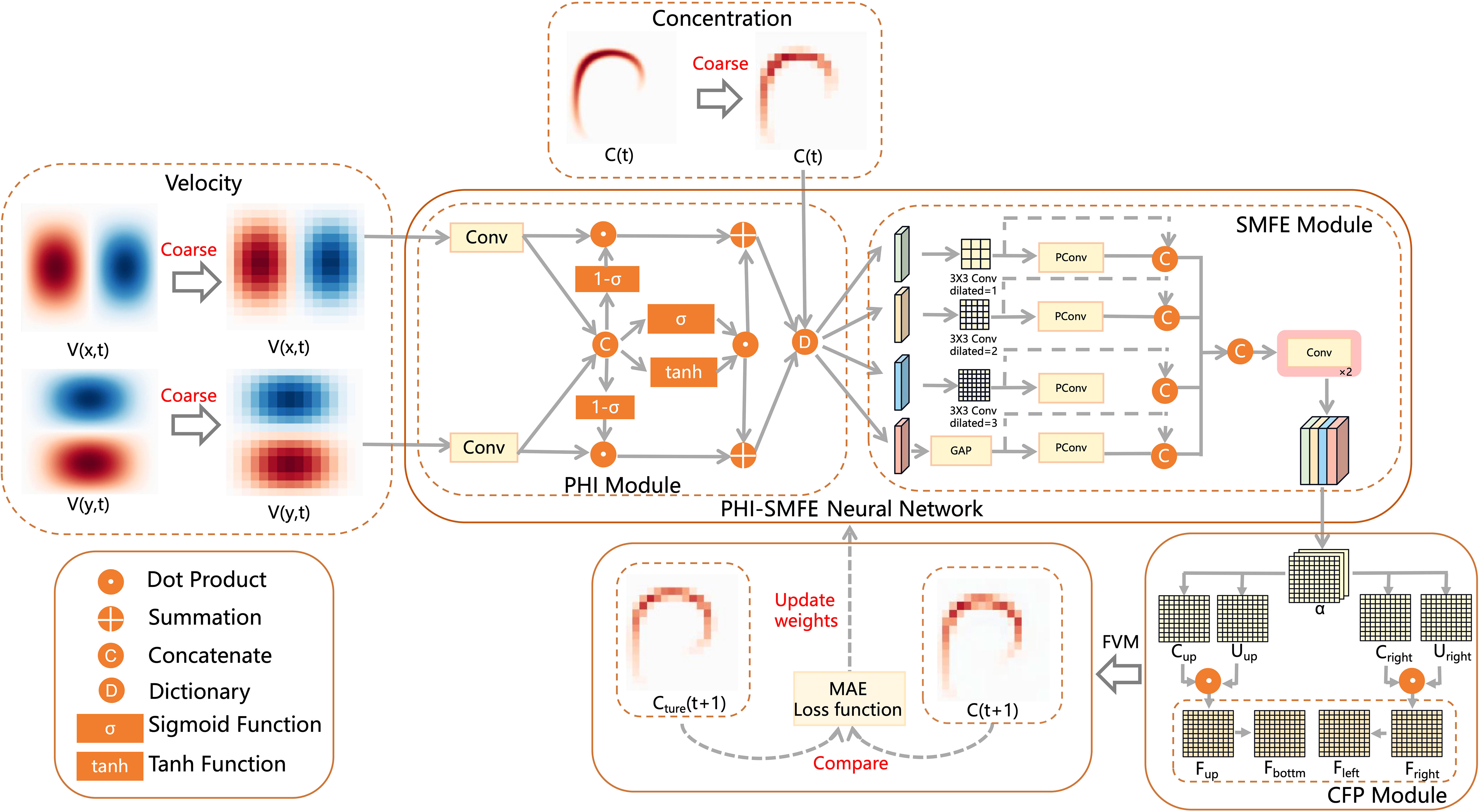
Figure 1 Our proposed PHI-SMFE neural network architecture. PHI module, SMFE module, and CFP module are the abbreviations of Physical heterogeneous interaction module, Spatial multi-scale feature extraction module, and Concentration field prediction module, respectively. The input velocity field and concentration field at the current moment pass through the above three modules in turn to obtain the concentration field at the next moment.

$\begin{array}{ll}\overrightarrow{\alpha }=f(U,C,W)& (1)\end{array}$

As depicted in formula (1), the spatial discretization coefficient $\overrightarrow{\alpha }$ encompasses various elements with physical significance, including velocity field templates U in both the horizontal and vertical directions, the concentration dynamic field C aligned with the direction of the velocity field, and trainable parameters W.

Subsequently, the two-dimensional velocity field and concentration field under the coarse grid are fed into PHI-SMFE for feature extraction. The network comprises two sub-modules: the physical heterogeneity interaction module (PHI) and the spatial multi-scale feature extraction module (SMFE). PHI module utilizes a 3×3 size two-dimensional periodic convolution to preprocess the velocity dynamic field in the X and Y directions, as well as the concentration dynamic field. The purpose of this preprocessing step is to enhance the heterogeneity in the characteristics of the dynamic field. Then, the correlation between the velocity dynamic field in the X and Y directions is enhanced through the nonlinear fusion, resulting in an interaction feature. Next, the interaction feature is combined with the concentration field feature through splicing. SMFE module receives the spliced features obtained from the previous module and utilizes convolution filters with varying dilated ratio to extract multi-scale features of the physical dynamic field. To tackle the computational complexity of the model, this module selectively performs convolution operations on specific channels of the features. This selective approach is employed due to the potential presence of redundant feature information in the expanded channels. By adopting this selective processing strategy, the inference process is accelerated. Next, the multi-scale features are concatenated, and two layers of conventional convolution are applied to obtain spatial discretization coefficient with the same number of channels as the number of flux templates. In the subsequent finite volume format module, these coefficients are divided into two parts to calculating the concentration field at the next time step. In the subsequent step, the CFP module calculates the concentration flux template using the spatial discretization coefficients obtained from the previous module, thereby obtaining the spatial derivative of the concentration field. The time derivative is computed using the finite volume scheme in the traditional solver to determine the concentration field for the next time step. Finally, a corresponding loss function is employed to minimize the discrepancy between the concentration dynamic field and update the learning parameters for the subsequent iteration of the network model.

Our proposed numerical simulation process for the passive scalar concentration dynamic field at the next time step can be summarized in the following three steps.

1) Utilize the proposed network model to extract multi-scale features from the velocity and concentration dynamic fields following data-driven discretization.

2) Perform the summation of the inner product between the spatial discretization coefficient and the concentration field template to obtain the spatial derivative.

3) Use the finite volume format module to calculate the time derivative and obtain the concentration field at the next time step using the forward Euler formula.

In the following subsections, we will provide detailed introductions to the two sub-modules of the proposed neural network model in Section 3.2 and Section 3.3, respectively. We will then discuss the spatial derivative calculation module in Section 3.4, followed by an explanation of the loss function used in Section 3.5.

3.2 Physical heterogeneous interaction module

The PHI module is specifically designed to incorporate the heterogeneity and correlation of various physical dynamic fields into the model. Taking the analysis of the velocity dynamic field as an example, we initially employ a 3×3 size convolution to amplify the nonlinearity of the velocity field characteristics. This step aims to enhance the network model"s capacity to capture the heterogeneity of the velocity field. Next, we concatenate the preprocessed features of the velocity dynamic field in the X and Y directions along a specified dimension to enable the modeling of feature correlations. Subsequently, we apply distinct nonlinear mapping functions to process the concatenated features. The specific calculation process is as follows.

$\begin{array}{ll}k=Tanh(Concat(\varphi (U(x,t)),\phi (U(y,t))))& (2)\end{array}$

$\begin{array}{ll}j=sigmoid(Concat(\varphi (U(x,t)),\phi (U(y,t))))& (3)\end{array}$

$\begin{array}{ll}i=1-sigmoid(Concat(\varphi (U(x,t)),\phi (U(y,t))))& (4)\end{array}$

Where, U(x,t) denotes the velocity field in the horizontal direction at the current time step, while U(y,t) represents the velocity field in the vertical direction at the current time step. ϕ and φ represent convolution operators for different dynamic fields. Additionally, i, j, and k denote the features obtained through different nonlinear mapping functions. Although the mapping ranges of these three nonlinear functions are comparable, each function serves a distinct purpose.

After performing the aforementioned operations, we compute the interaction between feature i and the dynamic feature of the original velocity field o, denoted as M-O Feature. This fusion process aims to enhance the existing effect of the original features, which already exhibit a relatively high level of effectiveness. Similarly, we fuse feature j after applying the Sigmoid mapping function and feature k after applying the Tanh mapping function, denoted as S-T Feature. By combining the respective advantages of these two mappings, the resulting features capture more complex nonlinear interactions and contain richer interaction information. Finally, we fuse the original inter-mapping interaction features (M-O) with the inter-mapping interaction features (S-T) to obtain the final heterogeneous-correlation integrated feature information, denoted as $S_{v_x}$ and $S_{v_y}$. The specific process is as follows.

$\begin{array}{ll}{S}_{v_x}=i\odot o_x+j\odot k& (5)\end{array}$

$\begin{array}{ll}{S}_{v_y}=i\odot o_y+j\odot k& (6)\end{array}$

In contrast to the analytical velocity dynamic field, we only employ a 3×3 size convolution operation to enhance the heterogeneity of the concentration dynamic field. denoted as S_c, Subsequently, we combine these enhanced features with the previously obtained integrated features of the velocity dynamic field. This fusion process yields the final set of features representing the physical dynamic field.

$\begin{array}{ll}I=dict(S_{v_x},S_{v_y},S_c)& (7)\end{array}$

The obtained feature set I serves as latent features for the SFME module, which will be elaborated upon in the subsequent section.

3.3 Spatial multi-scale feature extraction module

In fluid dynamic systems, the energy cascade or inverse cascade effect (Boffetta and Ecke, 2012) leads to the exchange of energy between vortices of varying scales. This phenomenon gives rise to the presence of intricate and multiscale features within the dynamic system. To effectively handle the complexity of such systems, it is advantageous to employ convolutional filtering with richer receptive fields. Motivated by this understanding, we introduce a pivotal sub-module in our network architecture, referred to as the SMFE module. The SMFE module takes as input the extracted potential features obtained from the PHI module. It employs convolution filters with various dilated ratio to extract features of diverse scales within the potential field simultaneously. This parallel extraction process allows for the capture of information at multiple spatial scales.

$\begin{array}{ll}{K}_i=k_i+(k_i-1)(d_i-1)& (8)\end{array}$

$\begin{array}{ll}{r}_n=r_{n-1}+(k_n-1){\displaystyle {\prod }_{i=1}^{n-1}{s}_i}& (9)\end{array}$

In formula (8), k_i represents the size of the original convolution kernel, K_irepresents the size of the expanded convolution kernel, and d_i represents the dilated ratio. Formula (9) calculates the receptive field size of the current layer based on the size of the expanded convolution obtained in the previous step. In this equation, s_i represents the stride number of the current layer, k_n represents the convolution kernel size of the current layer, r_n−1 represents the receptive field size of the previous layer, and r_n represents the receptive field size of the current layer. Applying formula (8) and formula (9) helps us determine an appropriate dilated ratio for measuring the scale range in the feature extraction task. In our case, the size of the discretized grid is 16∗16. After careful consideration, we select dilated ratio of 1, 2, 3 respectively.

$\begin{array}{ll}{M}_i=Dconv(I,d_i)& (10)\end{array}$

In formula (10), Dconv(·) represents the dilated convolution operator. The latent representation feature I undergoes the Dconv(·), resulting in the corresponding multi-scale features M_i(i = 1, 2, 3, 4).

To address the potential issue of redundant feature information in the feature extraction process, we introduce a batch-processing approach for channel features. This approach involves utilizing both dilated convolution and channel-biased convolution operators (Chen et al., 2023). The dilated convolution operator is applied to a portion of the channel features, while the channel-biased convolution operator is employed for the remaining channels. As shown in formula (11), the channel-biased convolution operator, based on feature selection, preserves the original features of certain channels while applying the convolution operator to process the features in the remaining channels. The resulting features from both operators are then concatenated in the channel dimension, yielding the feature set denoted as P_i(i = 1,2,3,4). This strategy effectively mitigates redundant feature information while maintaining the necessary computational efficiency.

$\begin{array}{ll}{P}_i=Concat(I,Conv(I_r))& (11)\end{array}$

Lastly, we combine the feature sets M_iand P_iby concatenating them along the channel dimension. The process is shown in formula (12). To ensure compatibility with the subsequent steps, we restore the number of channels to match the number of flux templates. This is achieved through two layers of conventional convolution. The obtained result is the spatial discretization coefficient, which plays a crucial role in our downstream inference tasks. The primary objective of our network is to learn and update this coefficient, enabling it to adaptively capture the spatial characteristics of the physical dynamic field.

$\begin{array}{ll}\alpha =Conv(Concat(M_i,P_i))& (12)\end{array}$

3.4 Concentration field prediction module

The proposed concentration field prediction (CFP) module is grounded in the finite volume method (Jameson et al., 1981), which is dependent on the dynamic field flux template. This module calculates the predicted dynamic field based on the obtained spatial discretization coefficients, adhering to two key principles.

Prediction based on the current state: The concentration field for the next time step is solely predicted using the current state, without considering future information.

Euler framework for derivative calculation: The discretized spatial derivative is computed using the explicit forward Euler method. This framework ensures that the derivative calculation on the divided grid strictly follows the Euler method. The original formula for the calculation is presented in formula (13).

$\begin{array}{ll}{\frac{\partial C}{\partial x}|}_{x=x_i}={\displaystyle {\sum }_{j=-k}^k{\alpha }_j{C}_{i+j}}& (13)\end{array}$

The spatial derivative of the discretized concentration dynamic field at the current moment is denoted as $\frac{\partial C}{\partial x}.\left\{x_1,\dots ,x_n\right\}$ represents the discretized spatial grid points, $\left\{a_{-k},\dots ,a_k\right\}$ is the matrix of discretized difference coefficients, and C_jdenotes the concentration at grid point x_j. By employing a variant of the original Euler method, we calculate the corresponding flux template. This method involves separately obtaining the dynamic templates for the vertical and horizontal dimensions, utilizing a split operator approach. This allows for the extension to the numerical solution of the two-dimensional equation.

$\begin{array}{ll}{F}_r=SUM(U_r\odot C_r)& (14)\end{array}$

$\begin{array}{ll}{F}_t=SUM(U_t\odot C_t)& (15)\end{array}$

Where {U_r,U_t} and {C_r,C_t} represent the velocity and concentration dynamic field templates at the right and top boundaries, respectively, obtained after splitting the spatial discretization coefficients. By applying the forward Euler’s formula, we perform the inner product between the corresponding concentration field and velocity field. Using the SUM(·) function, we expand and sum the inner product values across each grid point in the first dimension. This process allows us to obtain the flux template {F_r,F_t} at the right boundary and top boundary. Similarly, the corresponding flux {F_l,F_b} at the left boundary and bottom boundary can be obtained based on the computed flux.

Finally, adhering to the principle of dynamic continuity in the physical field, we utilize the obtained fluxes at the four boundaries to calculate the time derivatives.

$\begin{array}{ll}\frac{\partial C}{\partial t}=-\frac{(F_r-F_l)+(F_t-F_b)}{dx}& (16)\end{array}$

Where {F_r,F_t,F_l,F_b} represent the boundary flux templates in the right, top, left, and bottom directions, respectively, and dx represents the number of grid steps. By applying the forward Euler scheme, we can calculate the concentration dynamic field C_t+△t at the next time step using the time derivative $\frac{\partial C}{\partial t}$, the number of time steps dt, and the concentration field C_t at the current moment. This process allows us to update and predict the concentration dynamics over time based on the current state.

$\begin{array}{ll}{C}_{t+\mathrm{\Delta }t}=C_t+dt\frac{\partial C}{\partial t}& (17)\end{array}$

3.5 Loss function

We utilize the mean absolute value error (MAE) as both our loss function for model training and as a metric to evaluate the prediction confidence. The reason for selecting the MAE as the loss function is its robustness to extreme values and outliers in the forecast. This property ensures that extreme values resulting from numerical diffusion in the dynamic system do not disproportionately influence the forecast estimates. In addition, the conventional approach of estimating the conditional expected value as the prediction target is not well-suited for dynamic system prediction with an asymmetric error distribution. Instead, we propose using the approximate value of the conditional median as the prediction target. This approach allows us to capture the central tendency of the predicted values while accounting for the asymmetry in the error distribution. The specific formula is provided in formula (18).

$\begin{array}{ll}MAE=\frac{{\displaystyle {\sum }_{i=1}^n\left|{\widehat{C}}_{t+\mathrm{\Delta }t}-C_{t+\Delta t}\right|}}{n}& (18)\end{array}$

MAE is computed as the sum of the absolute differences between the observed values and the corresponding true values, divided by the sample size n. In our study, C_t+△t represents the predicted value of the concentration field at the next moment, while ${\widehat{C}}_{t+△t}$ refers to the reference solution, derived from executing the second-order Van Leer advection solver (Lin et al., 1994) evolving under initial concentration conditions.

4 Experiments

In the experimental section, we provide a comprehensive description of the implementation details and the data sets creation process. The generated data sets are constructed by introducing various types of divergence-free velocity dynamic fields, which alter the flow patterns within the same initial concentration dynamic field conditions. In the experimental phase, we conduct a comparative analysis between our proposed model and state-of-the-art (SOTA) models, as well as traditional finite-difference models. Additionally, we perform an ablation study specifically on our proposed model. The objective of these experiments is to evaluate and assess the performance of our model in terms of simulation accuracy and computational efficiency. The experimental results clearly demonstrate that our proposed model outperforms the competing models in terms of both accuracy and acceleration, validating its effectiveness and superiority in simulating fluid dynamic fields.

4.1 Implementation details

PHI-SMFE, along with other baseline models, was tested and trained using the NVIDIA Tesla V100SXM2 GPU. During the training process, we utilized the Adam optimization algorithm with a default learning rate of 10−3. We set the learning rate decay rate to 0, indicating that the learning rate remained constant throughout training. The input batch size during training was set to 40. To prepare the input physical dynamic field, we applied a spatial grid coarsening method to downsample the original velocity dynamic field dataset and concentration dynamic field dataset from a grid resolution of 128*128 to a resolution of 16*16. Subsequently, the low-resolution raw dataset was split into separate training and testing sets. Both the training set and the test set were divided into two parts: a pre-inference input part and a post-inference output part. The input part before inference consisted of the velocity field and concentration field at the current time t, while the output part after inference contained the concentration field at the next time t+1. In the SMFE module, the dilated convolution layer and the channel-biased convolution layer are configured with 20 filters each, while the pooling layer utilizes 40 filters. During the training process, all network layers have their weights randomly initialized. The total size of the network model is 11.2k, and the size of the training weight parameters amounts to 61.4k.

4.2 Data sets

4.2.1 Random velocity dynamic field

The generation of random velocity dynamic fields follows the theory of non-divergent velocity field calculation (Kraichnan, 1970). According to this theory, it is essential to ensure that the two velocity component vectors are perpendicular to each other in order to achieve a non-divergent velocity field. This requirement guarantees the proper implementation of the non-divergence condition in the generated velocity fields. We obtain the final random velocity dynamic field by computing the horizontal velocity field component and the vertical velocity field component for each point on the designated 128x128 discretization grid. The calculation process of the velocity field is as follows.

$\begin{array}{ll}u(x)={\displaystyle {\sum }_{n=1}^N{w}_n}\sin (k_{n}x+w_{n}t)+{\displaystyle {\sum }_{n=1}^N{u}_n}\cos (k_{n}x+w_{n}t)& (19)\end{array}$

$\begin{array}{ll}u(y)={\displaystyle {\sum }_{n=1}^N{w}_n}\sin (k_{n}y+w_{n}t)+{\displaystyle {\sum }_{n=1}^N{u}_n}\cos (k_{n}y+w_{n}t)& (20)\end{array}$

Where the variables v_n and w_n represent the amplitudes determined based on velocity divergence constraints. The wave number is denoted by k_n, while x and y represent the two-dimensional spatial positions within the current grid. The variable ω_n represents the frequency, and t corresponds to the time parameter. We generate random velocity dynamic fields over multiple time steps by evenly spacing the time parameter, resulting in a dataset with diverse temporal variations. To ensure the generalization performance of the model, we carefully partition the random velocity dynamic field dataset into distinct training and test set portions. This division guarantees that the model is exposed to different instances during training and evaluation.

4.2.2 Concentration dynamic field

To initiate the concentration dynamic field, we generate initial values within the range [0,1] for each point in the two-dimensional concentration field. To ensure the periodicity of the field, we apply a two-dimensional periodic boundary constraint. Next, we employ the second-order finite-difference Van Leer advection model to evolve the initial concentration field over time, taking into account the corresponding velocity dynamic field. This process results in snapshots of the concentration field at multiple time steps. Similarly to the velocity dynamic field dataset, we partition the concentration dynamic field dataset into separate training and test sets. This division ensures that the training and evaluation phases use distinct subsets of data, preserving the consistency between the concentration and velocity dynamic field datasets. The specific calculations for the initial concentration field are detailed in formulas (21)-(25).

$\begin{array}{ll}r(x,y)=4\sqrt{{(x-\frac{1}{4})}^2+{(y-\frac{1}{4})}^2,}r\in [0,1]& (21)\end{array}$

$\begin{array}{ll}{c}_1(x,y)=\frac{1}{2}(1+\cos (\pi r))& (22)\end{array}$

$\begin{array}{ll}{c}_2(x,y)=\frac{9}{10}-\frac{4}{5}{(c_1)}^2& (23)\end{array}$

$\begin{array}{ll}{c}_3(x,y)=\{\begin{array}{c}\frac{1}{10}{c}_1,r\ge \frac{1}{2}\\ 1,r<\frac{1}{2}\end{array}& (24)\end{array}$

$\begin{array}{ll}C(x,y)=1-\frac{3}{10}(c_1+c_2+c_3)& (25)\end{array}$

In the given equations, {x,y} represents the spatial coordinates of a two-dimensional grid point, indicating its position within the system. The function r denotes the boundary constraint, which imposes specific conditions on the behavior of the concentration dynamic field at the system boundaries. The constraints {c₁,c₂,c₃} specify the conditions that the initial concentration dynamic field must satisfy at different locations or boundaries. These conditions include specific concentration values or other constraints relevant to the problem. C(x,y) represents the initial concentration value assigned to each grid point, determining the starting state of the concentration dynamic field.

4.3 Comparison with SOTA methods

4.3.1 Results on unsteady dynamic fluid fields

We conducted experiments using an unsteady dynamic flow field dataset to compare the performance of the proposed PHI-SMFE model with the traditional SOTA numerical simulation Van Leer solver. The traditional numerical simulation baseline schemes selected for passive scalar advection under 2D unsteady flow include the following:(1)Second-order Van Leer advection transport scheme with a grid resolution of 16x16 (Lin et al., 1994). (2)Second-order Van Leer advection transport scheme with a grid resolution of 32x32 (Lin et al., 1994). (3)Second-order Van Leer advection transport scheme with a grid resolution of 64x64 (Lin et al., 1994). The superiority of the second-order Van Leer method in transporting fluids with steep gradients, while avoiding unrealistic oscillations and negative mixing ratios, is showcased in low-resolution atmospheric simulations involving active cumulus convection. This state-of-the-art scheme replaces the fourth-order central difference scheme (Li et al., 1995) and has been implemented in the simulation of the general circulation of the atmosphere at the Goddard Laboratory. Figure 2 illustrates the comparative outcomes of the cumulative errors over multiple time steps between the PHI-SMFE model and the Van Leer method.

FIGURE 2

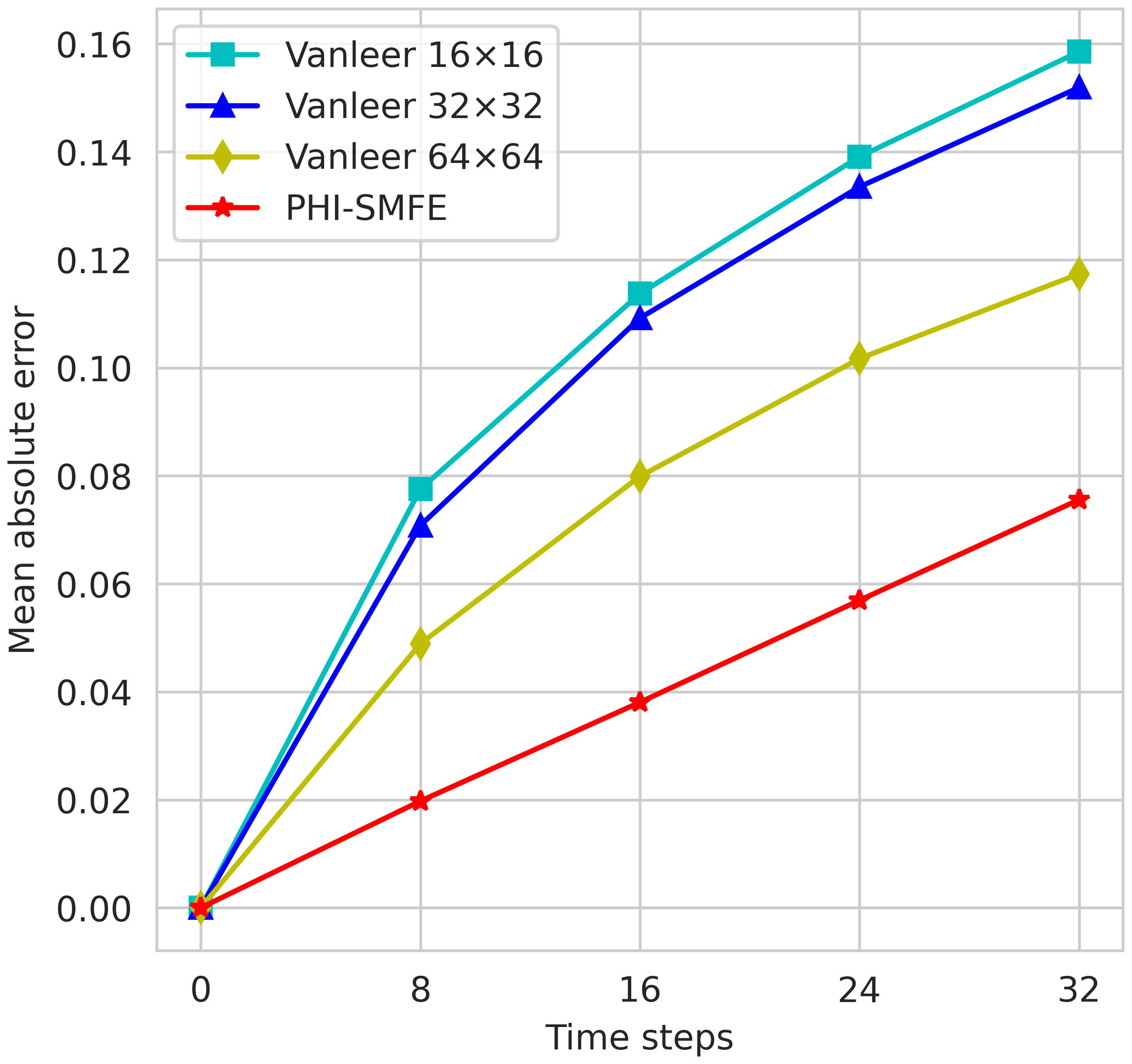
Figure 2 Accuracy simulation results of the traditional competitive model and the proposed PHI-SMFE model at 32-time steps in a unsteady fluid field dataset.

The results clearly demonstrate that our PHI-SMFE model, trained on a 16*16 grid resolution, consistently achieves the lowest prediction error across 32-time steps. This substantiates the superiority of our proposed method in enhancing the accuracy of fluid numerical simulation. Notably, the prediction error of PHI-SMFE at the 32nd time step is 0.079, significantly outperforming the traditional solution model. This finding highlights the capability of our proposed method to achieve higher numerical solution accuracy at a grid resolution four times lower than that of the conventional SOTA numerical simulation scheme.

Subsequently, we conducted a comparative analysis between PHI-SMFE and a state-of-the-art deep learning-based spatially discretized CNN-FVM solver (Zhuang et al., 2021). The CNN-FVM approach employs a fusion framework that seamlessly integrates neural network modules into traditional finite volume schemes. Extensive research has demonstrated the ability of this method to achieve advanced simulation accuracy and acceleration in numerically solving various equations, including the Burgers equation (Bar-Sinai et al., 2019), advection equation (Zhuang et al., 2021), and incompressible NavierStokes equation (Kochkov et al., 2021). In the low-resolution advective transport simulation, which is represented by the advection equation, this method demonstrates an accuracy comparable to that of the traditional second-order flux-limited advection solver, even when using a grid that is four times coarser. In the direct numerical simulation of high-resolution turbulent flow governed by the incompressible NavierStokes equations, this method achieves a simulation accuracy comparable to that of the DNS baseline solver, even when using a grid resolution that is 8 to 10 times coarser. This remarkable accuracy is accompanied by a significant computational acceleration, reaching a speedup of 40 to 80 times compared to the baseline solver.

Our experimental comparison focuses on the advection of passive scalar in 2D turbulent flow. Specifically, we evaluate the performance of our proposed PHI-SMFE model against the baseline method CNN-FVM. In terms of single-step prediction, the CNN-FVM method achieves an inference error of 0.0044 and an inference time of 0.1781s. The average training time per epoch during the training phase is 4ms. On the other hand, our PHI-SMFE model achieves an improved performance with an inference error of 0.0027, an inference time of 0.0752s, and an average training time of 450us per epoch. Overall, our PHI-SMFE model demonstrates a significant enhancement in both single-step simulation accuracy, which has increased by 38%, and single-step inference speed, which has improved by 58%. These results position our model at the forefront of the current state-of-the-art performance. Additionally, we conducted tests to evaluate the cumulative loss over multiple time steps. The comparison of multi-step cumulative errors between PHI-SMFE and CNN-FVM is illustrated in Figure 3. The results demonstrate that PHI-SMFE exhibits a more gradual cumulative growth of error compared to the baseline Conv-FVM. Additionally, the overall loss at 32-time steps is reduced by 41% in PHI-SMFE, indicating its capability to significantly enhance simulation inference accuracy across multiple time steps.

FIGURE 3

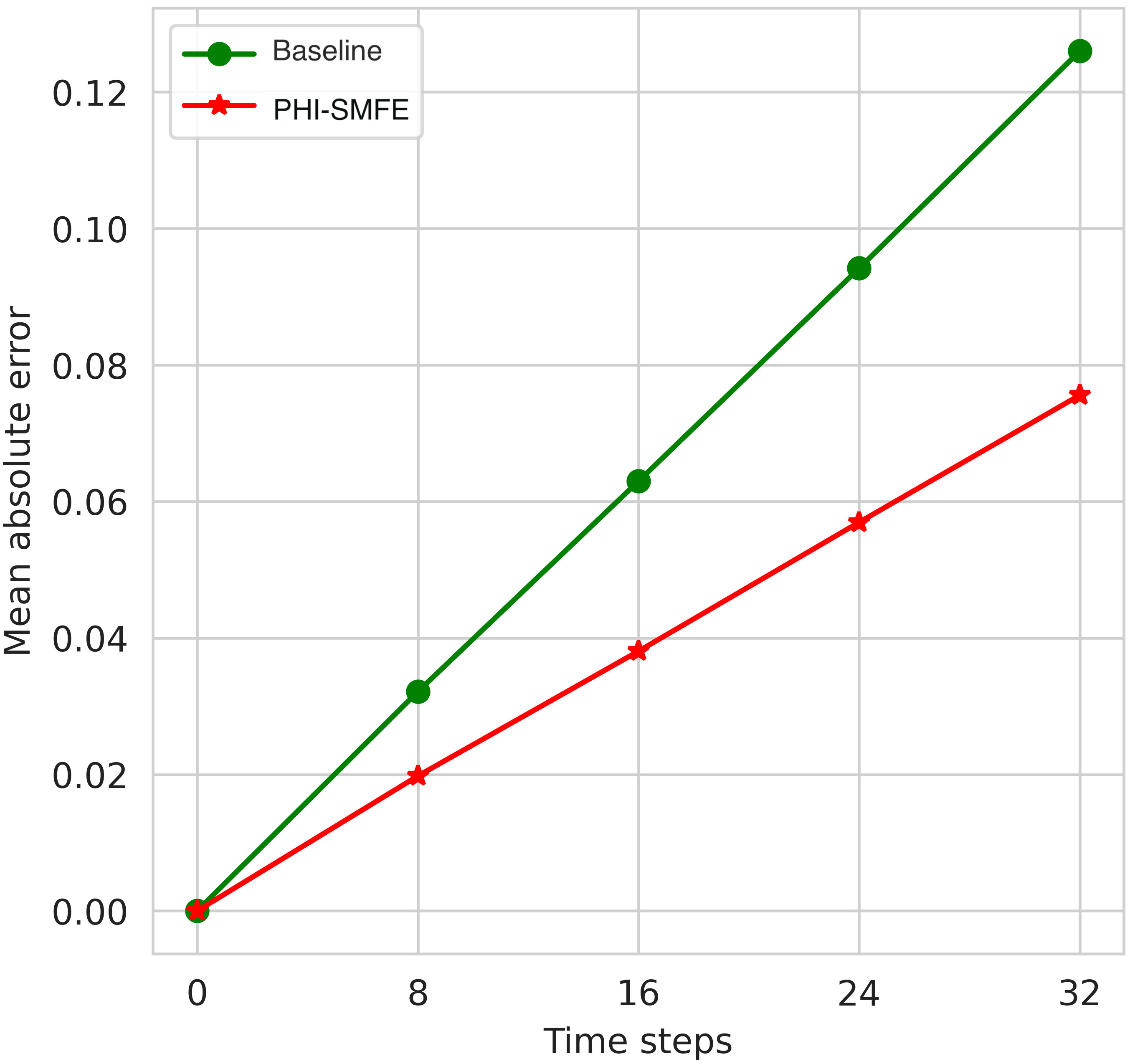
Figure 3 Accuracy simulation results of the deep learning competition model and the proposed PHI-SMFE model at 32-time steps on a unsteady fluid field dataset.

Furthermore, we conducted tests to evaluate the multi-time step inference speed of the proposed method and the SOTA model. Figure 4 illustrates the results, indicating that the baseline method requires a total running time of 0.7665s for multi-time step inference, while the proposed PHI-SMFE achieves a total running time of 0.6693s. This represents a notable reduction of 12.7% in running time compared to the baseline method. Considering that the model requires re-invoking the solver for inference at each time step, we believe that evaluating inference performance in the multi-sample case can provide a better indication of the accelerated computing power of the proposed model. This concept aligns with the findings observed in the single-step inference test described earlier. The superior acceleration performance of our proposed model compared to the baseline can be attributed to several factors. Firstly, in the spatial discretization coefficient prediction component, PHI-SMFE reduces the depth of the original model by employing a single layer of multi-scale pyramid network and two layers of convolutional network to handle dynamic field features. This reduction in model depth leads to significantly smaller trained model parameters compared to the original model. Additionally, PHI-SMFE minimizes redundant processing in scale feature extraction, and the lateral connections in the network layers retain feature information from previous layers in a channel-biased manner. The weight quantization index further supports the enhanced computational acceleration of our proposed model. Specifically, the weight parameters of the original model amount to 7.93MB, whereas the trained model’s weight parameters are only 61.4kB in size.

FIGURE 4

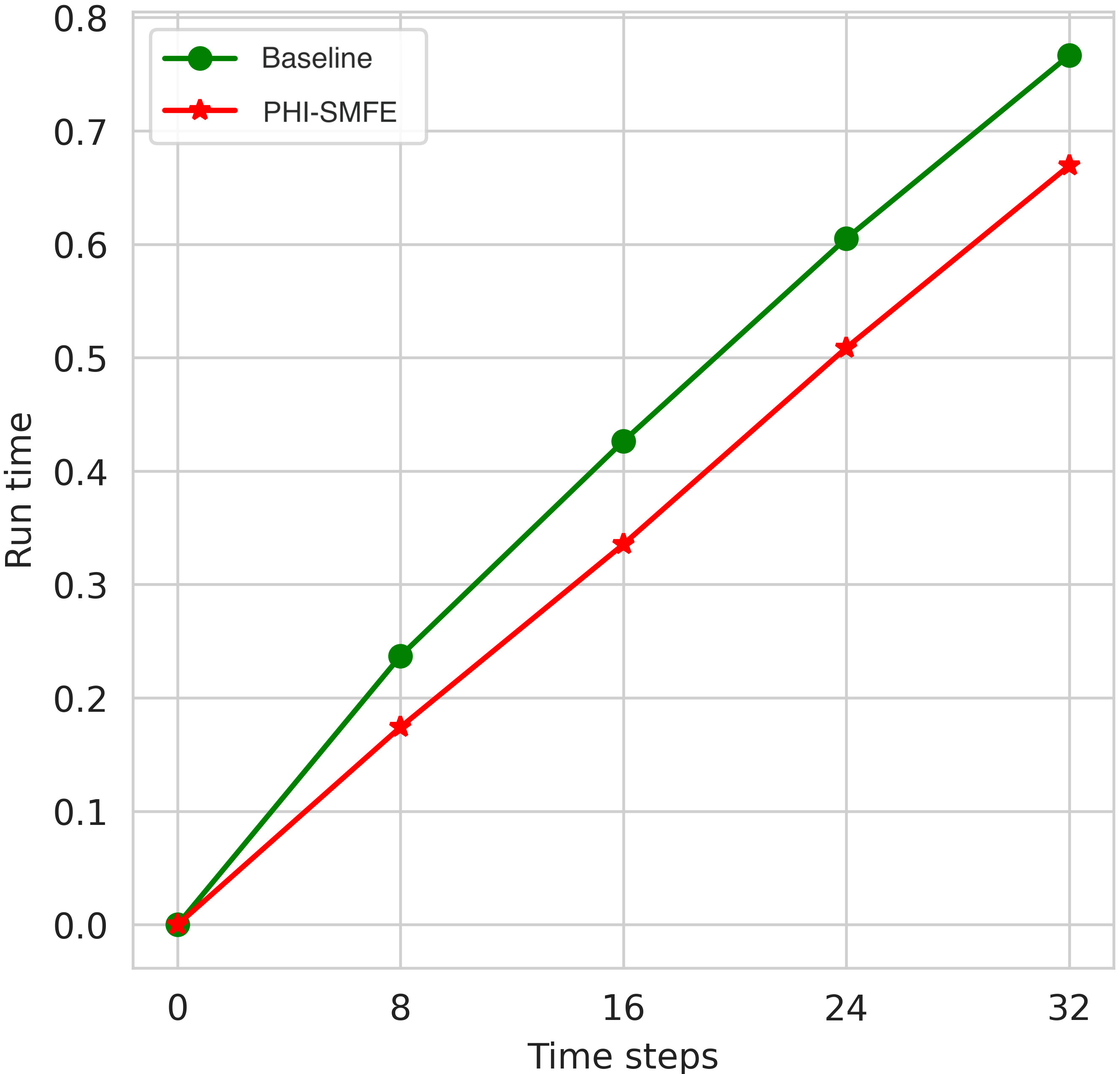
Figure 4 The simulation results of the solution speed of the deep learning competition model and the proposed PHI-SMFE model under the unsteady fluid field dataset under 32-time steps.

We further provided visualizations of the results obtained by different models in the inference of the numerical evolution of the concentration field. Figure 5 illustrates these visualizations, showcasing the behavior of each model as the time step increases. It is evident that the inference results of the traditional finite-difference scheme model exhibit a significant amount of invisible diffusion when operating under a low-resolution grid. This observation indicates that the performance of the traditional model is inadequate and fails to provide satisfactory simulation results. Similarly, the Conv-FVM model also displays some numerical diffusion in the numerical simulation of the concentration field, suggesting that the model lacks stability. In contrast, our PHI-SMFE Network model surpasses the performance of the aforementioned models, producing inference results that align more closely with the actual simulation scenario.

FIGURE 5

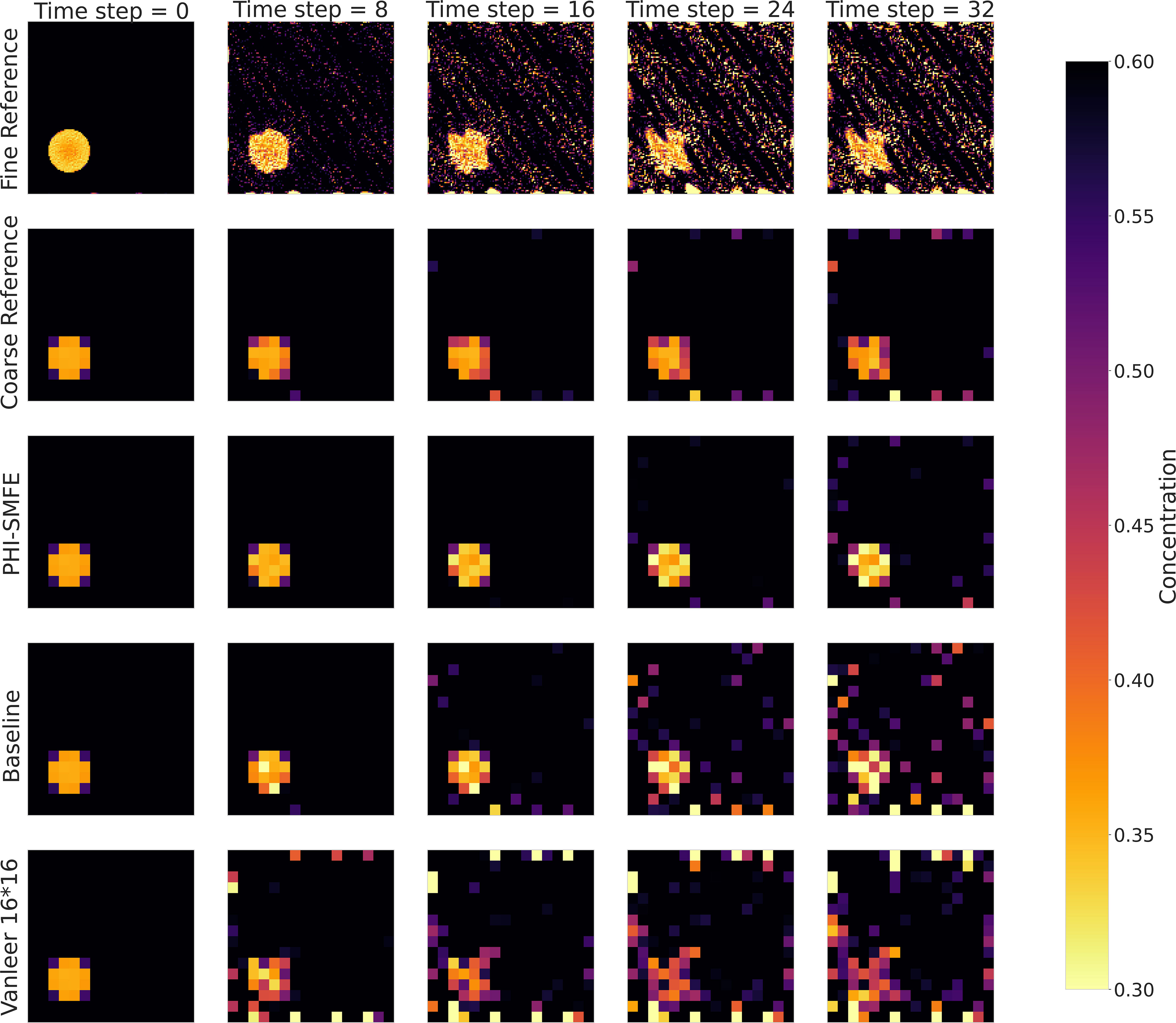
Figure 5 Visualization of predictions of the evolution of the initial concentration field after 32 time-step iterations of different models under a unsteady fluid field dataset. The third row represents the prediction results of the proposed PHI-SMFE model.

4.3.2 Results on other fluid fields

We conducted an evaluation of the simulation performance of the PHI-SMFE neural network on additional fluid dynamic field datasets, namely the constant flow dynamic field dataset and the deformation flow dynamic field dataset. For the constant flow dynamic field dataset, the velocity field values at each grid point remain constant throughout the simulation, and the initial concentration field is set to match that of the unsteady flow initial concentration field. On the other hand, the deformation flow dataset serves as a standard test field for atmospheric advection schemes, featuring a velocity field composed of periodic eddies. The specific calculation formulas for the deformation flow dataset can be found in formulas (26) and (27).

$\begin{array}{ll}u(x,y,t)={\text{=sin}}^2(2\pi x)\sin (2\pi y)\cos (\frac{\pi t}{T})& (26)\end{array}$

$\begin{array}{ll}u(x,y,t)={\text{sin}}^2(2\pi y)\sin (2\pi x)\cos (\frac{\pi t}{T})& (27)\end{array}$

Where the period is denoted by T. It is worth noting that the velocity dynamic field at time t = nT remains consistent with the initial velocity dynamic field. The initial concentration field takes a circular shape, and its calculation formula is provided in formulas (28) and (29).

$\begin{array}{ll}r(x,y)=4\sqrt{{(x-\frac{1}{4})}^2+{(y-\frac{1}{4})}^2,}r\in [0,1]& (28)\end{array}$

$\begin{array}{ll}C(x,y)=\frac{1}{2}(1+\cos (\pi r))& (29)\end{array}$

Under the conditions of the constant flow velocity field and the deformed flow velocity field, we performed time evolution of the initial concentration fields to generate the constant flow concentration dynamic field and the deformed flow concentration dynamic field, respectively. The visual simulation inference results under time evolution are presented in Figures 6 and 7. It can be observed that our model performs well in the inference of the deformed flow under the 32-step time iteration, exhibiting good agreement with the observed reality. However, in the results of the constant flow dynamic field simulation, it is evident that the concentration field at the 24th time step exhibits slight deviation signs, and the concentration field at the 32nd time step displays a slight trajectory drift. This can be attributed to the accumulation of errors as the number of iterations increases, resulting in poorer inference results. The experimental findings indicate that there is still ample room for improvement in our proposed model, and we will explore solutions to address this issue in future research endeavors.

FIGURE 6

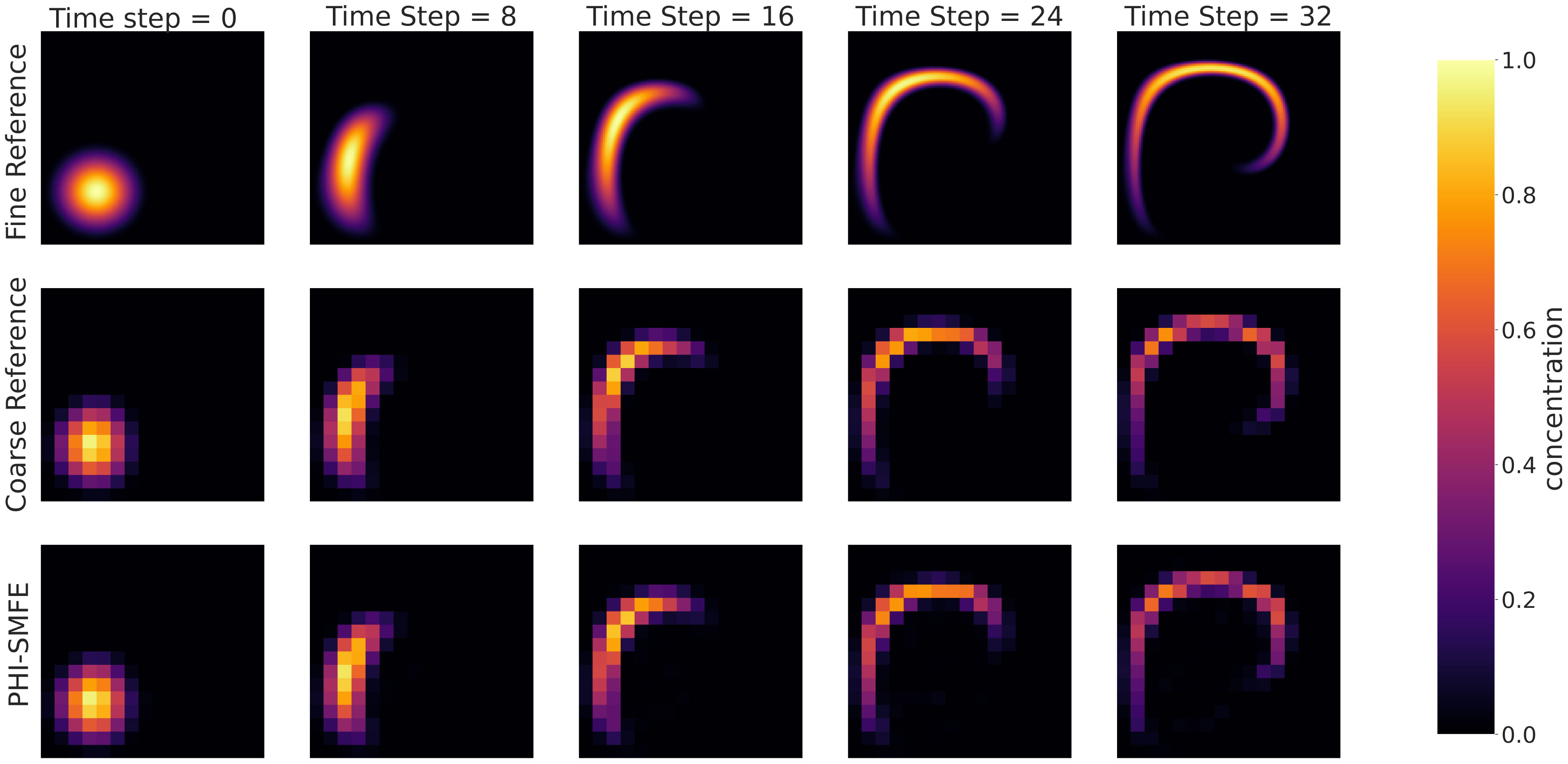
Figure 6 Visualization of iterative evolution predictions for different models under deformed flow field datasets. The third row represents the prediction results of the PHI-SMFE model.

FIGURE 7

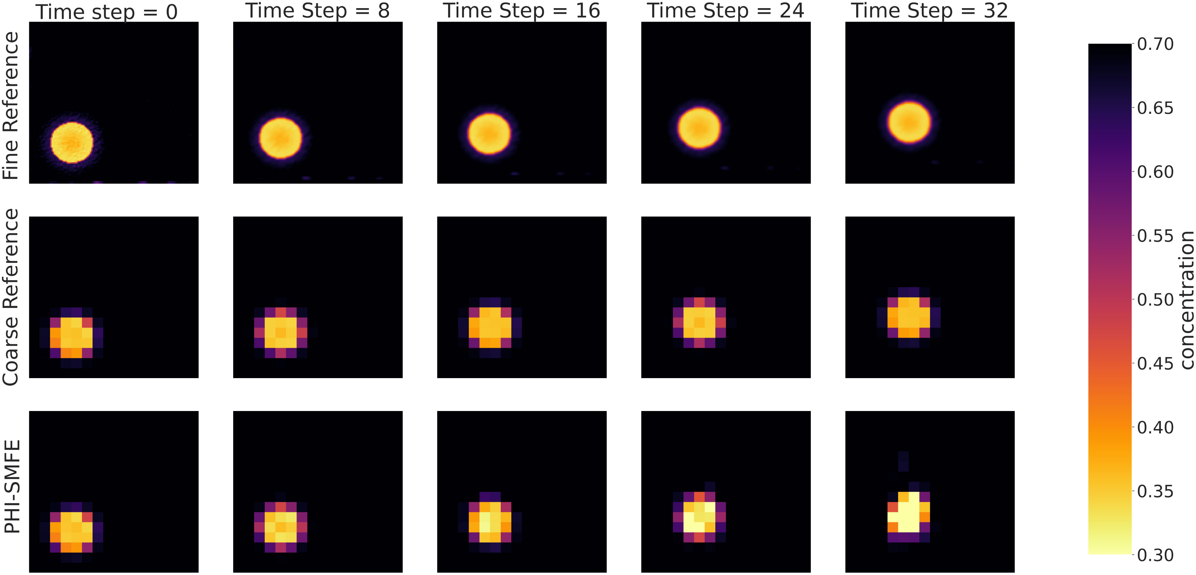
Figure 7 Visualization of Iterative Evolution Prediction of Different Models under Constant Flow Field Dataset. The third row represents the prediction results of the PHI-SMFE model.

4.4 Ablation study

Within the realm of machine learning, ablation study is geared towards the examination of specific components within a network model. This approach seeks to gain deeper insights into the network model’s behavior by selectively deactivating or altering certain parts of it. This section focuses on examining the impact of PHI modules and varying dilation coefficients on the accuracy of numerical simulation for passive scalar advection. Additionally, we investigate the effectiveness of channel-biased convolution in improving the computational performance of numerical simulations. The evaluations and metrics presented in this section are conducted using unsteady dynamic field datasets. It should be noted that the Contrast model in Figures 8–10 refer to the comparison models after ablation of the specified modules.

FIGURE 8

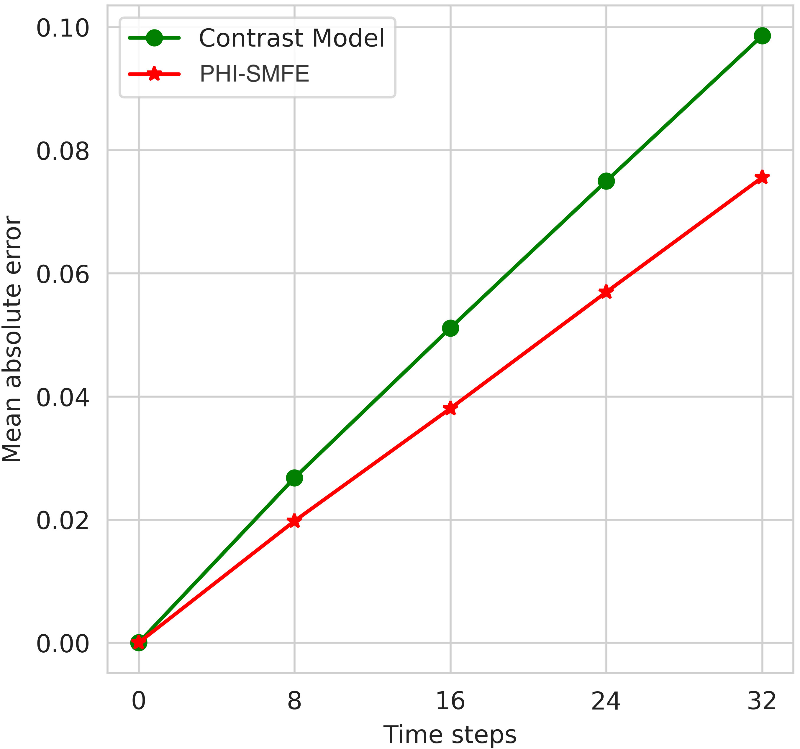
Figure 8 Accuracy simulation results with and without PHI fusion model under unsteady fluid field dataset.

FIGURE 9

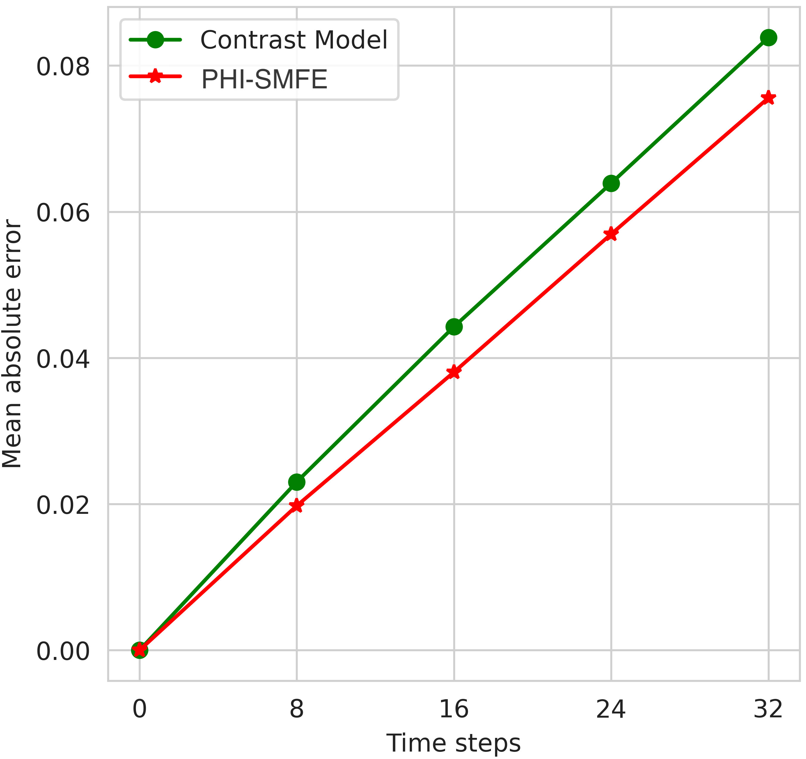
Figure 9 Accurate simulation results of the model with and without the separation strategy under a unsteady fluid field dataset.

FIGURE 10

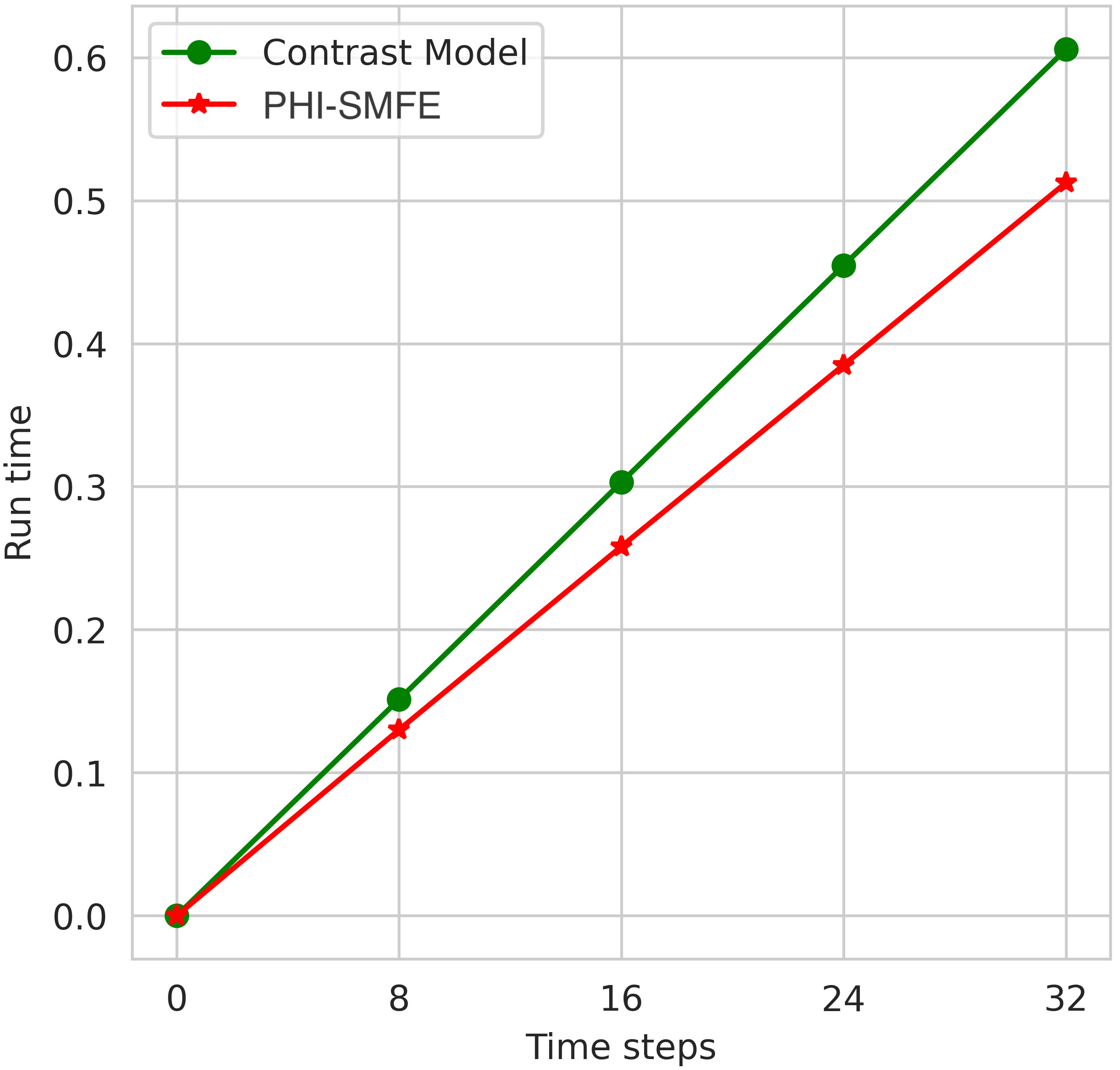
Figure 10 Solution speed simulation results of the model with and without a separation strategy under a unsteady fluid field dataset.

4.4.1 Impact of PHI module for simulation of unsteady dynamic field

Considering the correlated nature of different physical dynamic fields, our PHI module aims to improve the heterogeneity of physical dynamic fields and the correlation between them, thereby enabling better simulations. Therefore, we ablated the PHI module, trained two models with and without the PHI module, and verified the superior performance of the PHI module by comparing the performance indicators of the ablated Contrast model and PHI-SMFE in numerical simulation tests. The test results are shown in Figure 8, from which it can be seen that the proposed PHI-SMFE obtains a lower cumulative error in time step iterations, which also indicates the best simulation performance.

We illustrate the reasons for these results by pointing out the shortcomings of the Contrast model and the advantages of PHI-SMFE, respectively. The Contrast model using the convolutional filter fusion strategy provides inferior simulation accuracy (23%) since the fact that the convolutional filter fusion strategy of the baseline method Conv-FVM only uses an increased number of channels to fuse the feature information after splicing velocity field and concentration field, which does not effectively enforce global correlation between velocity and concentration field features, resulting in poorer simulation guidance. On the contrary, the PHI module uses a shunt strategy before performing the correlation between the velocity field and the concentration field. By separately performing pre-feature extraction on different dynamic fields, the learning model can understand the unique heterogeneous information of different physical fields. The subsequent fusion strategy implements the nonlinear global interaction between the velocity field and the concentration field features, which strengthens the representation ability of the intermediate features and improves the simulation accuracy by 21%. This verifies that the PHI module is an effective fusion method for the numerical simulation of the flow field.

4.4.2 Impact of different dilated ratio for simulation of unsteady dynamic field

Due to the uncertainty in the scale of the fluid dynamic field features, the model performance will be affected by the limitation of the scale processing range of the dilated convolution in the SMFE module. We performed a heuristic search on the hyperparameters of the model. Under different dilated ratio, the model can extract features with different scale ranges to predict discretized difference coefficients. The best prediction results represent that the scale extraction range of the model can better match the scale size of the physical dynamic field characteristics under the selected dilated ratio, so as to obtain the optimal difference coefficient. The coarsened physical dynamic field is executed under the grid size of 16 ∗ 16, which limits the scaling processing to be within a reasonable range of the matching grid size. In other words, the range of dilated ratio we need to consider exists in a bounded within the collection. The size of our convolution kernel is 3 × 3. According to the calculation formulas (8)-(9), when the dilated ratio is 7, the receptive field size reaches the boundary range of the grid. This extrapolation provides a reasonable guide for choosing dilated ratio. Finally, we set three different dilated ratio to extract small-scale, medium-scale, and large-scale fluid features. The optimal dilated ratio is determined through the tests illustrated in Figure 11. It can be seen that the iterative simulation achieves the best results when the dilated ratio are {1 ,2, 3} respectively. When the scale range that the convolution can handle gradually increases, the simulated iterative loss gradually decreases, but it is still not as good as when the dilated ratio are {1, 2, 3}. At the same time, considering that the convolution operator with a large receptive field may bring unnecessary tensor calculations, increasing the computational burden. We choose {1, 2, 3} as the final set of dilated ratio used by the model.

FIGURE 11

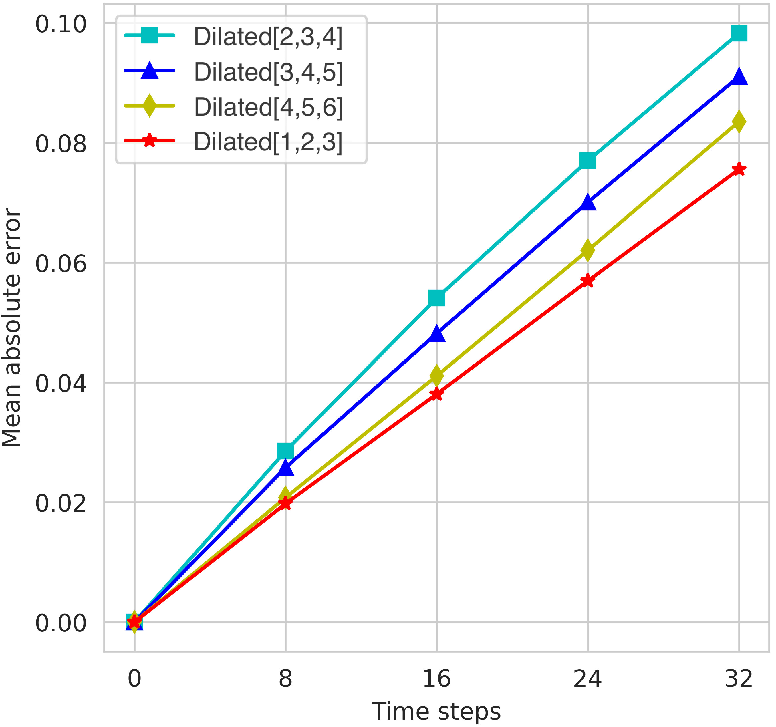
Figure 11 Accuracy simulation results of different dilated ratio models and PHI-SMFE model under the unsteady fluid field dataset.

4.4.3 Effectiveness of separation strategy for simulation of unsteady dynamic field

In this section, we evaluate the effect of channel-biased convolution in model-guided learning of discretized differential coefficients. We replace the channel-biased convolution operator in PHI-SMFE with ordinary convolution to obtain the Contrast model, and compare the corresponding numerical simulation results and inference time on the unsteady dynamic flow field. From Figure 9, we observe that the Contrast model using ordinary convolutions exhibits limited simulation performance because the redundant feature information produced by the model will accumulate with the increase of network layer depth. By adding side-channel convolution to the learning model, the accuracy of the final numerical simulation is improved by 5%, which shows that the side-channel convolution operator is beneficial to the learning of discretized difference coefficients. From Figure 10, we observe that SMFE module using channel-biased convolution can effectively accelerate simulation inference because, in each feature extraction, channel-biased convolution retains part of the original feature information and thus reduces the need for redundant feature processing. In inference simulations, channel-biased convolution achieves a 16.7% computational speedup.

5 Conclusion

We propose a PHI-SMFE network for solving passive scalar advection in 2D unsteady flow and implement it in numerical simulations of three test cases. We use the network model to learn discretized differential coefficients, calculate the time partial derivative and spatial partial derivative related to the concentration dynamic field according to the learned adaptive differential coefficient, and then combine the traditional finite volume scheme to obtain a High-precision solution under the resolution grid.

To improve the accuracy of fluid numerical calculations, we have developed a feature extraction module based on different scales, called SMFE Module, which aims to capture the difficult-to-analyze scale turbulence feature information in complex fluid dynamic fields. At the same time, considering the interactive influence of the fluid velocity field on the concentration field, we designed the physical heterogeneous interaction module to enhance the heterogeneity of the physical fields and the nonlinear interaction between them. Furthermore, we propose a channel-biased convolution operator to speed up numerical computation by reducing the processing of redundant feature information. Compared with other deep learning models, our model achieves state-of-the-art performance in terms of reduced computational cost and improved accuracy.

Despite achieving state-of-the-art results, our proposed model still has limitations in reducing iteration errors, as shown in Figure 7. The trajectory drift problem occurs in the dynamic field at the end of the time step iteration. In addition, we need to combine it with the prediction of real data, and add the integration of neural networks and numerical solutions to partial differential equations in the prediction process. This can add physical information constraints to better solve real problems in atmospheric science and earth science. We will address these issues in future work.

Data availability statement

The raw data supporting the conclusions of this article will be made available by the authors, without undue reservation.

Author contributions

YY: Writing – original draft. NS: Conceptualization, Writing – review & editing. JN: Conceptualization, Supervision, Writing – review & editing. XS: Writing – review & editing. JC: Investigation, Validation, Writing – review & editing. QW: Conceptualization, Supervision, Writing – review & editing. ZW: Writing – review & editing.

Funding

The author(s) declare financial support was received for the research, authorship, and/or publication of this article. This work was supported in part by the National Key Research and Development Program of China (2021YFF0704000), Major Science and Technology Innovation Project of Shandong Province (2019JZZY020705), the National Natural Science Foundation of China (62172376), and Fundamental Research Funds for the Central Universities (202042008).

Acknowledgments

Thanks to Prof. Tian(Hao Tian, College of Mathematical Science, Ocean University of China, Qingdao, China) for his theoretical guidance and help. We are very grateful to Prof. Song (Dehai Song, Key Laboratory of Physical Oceanography, Ocean University of China, Qingdao, China) for providing us with data and ideological support and help.

Conflict of interest

The authors declare that the research was conducted in the absence of any commercial or financial relationships that could be construed as a potential conflict of interest.

Publisher’s note

All claims expressed in this article are solely those of the authors and do not necessarily represent those of their affiliated organizations, or those of the publisher, the editors and the reviewers. Any product that may be evaluated in this article, or claim that may be made by its manufacturer, is not guaranteed or endorsed by the publisher.

References

Alcouffe R. E., Brandt A., Dendy J. E., Painter J. W. (1981). The multi-grid method for the diffusion equation with strongly discontinuous coefficients. SIAM J. Sci. Stat. Computing 2, 430–454. doi: 10.1137/0902035

CrossRef Full Text | Google Scholar

Alfonsi G. (2009). Reynolds-averaged navier–stokes equations for turbulence modeling. Appl. Mechanics Rev. 62 (4), 040802. doi: 10.1115/1.3124648

CrossRef Full Text | Google Scholar

Arcoumanis C., Whitelaw J. (1987). Fluid mechanics of internal combustion engines—a review. Proc. Institution Mechanical Engineers Part C: J. Mechanical Eng. Sci. 201, 57–74. doi: 10.1243/PIMEPROC198720108702

CrossRef Full Text | Google Scholar

Arroyo C. P., Kholodov P., Sanjosé M., Moreau S. (2019). Cfd modeling of a realistic turbofan blade for noise prediction. part 1: Aerodynamics. Proc. Global Power Propulsion Soc. (GPPS 2019). GPPS-BJ-2019-0013 doi: 10.33737/gpps19-bj-126

CrossRef Full Text | Google Scholar

Bar-Sinai Y., Hoyer S., Hickey J., Brenner M. P. (2019). Learning data-driven discretizations for partial differential equations. Proc. Natl. Acad. Sci. 116, 15344–15349. doi: 10.1073/pnas.1814058116

CrossRef Full Text | Google Scholar

Bassi F., Rebay S. (1997). A high-order accurate discontinuous finite element method for the numerical solution of the compressible navier–stokes equations. J. Comput. Phys. 131, 267–279. doi: 10.1006/jcph.1996.5572

CrossRef Full Text | Google Scholar

Belbute-Peres F. D. A., Economon T., Kolter Z. (2020). “Combining differentiable pde solvers and graph neural networks for fluid flow prediction,” in international conference on machine learning (PMLR), (International Conference on Machine Learning), 2402–2411.

Google Scholar

Benmoshe N., Pinsky M., Pokrovsky A., Khain A. (2012). Turbulent effects on the microphysics and initiation of warm rain in deep convective clouds: 2-d simulations by a spectral mixed-phase microphysics cloud model. J. Geophysical Research: Atmospheres 117 (D6). doi: 10.1029/2011JD016603

CrossRef Full Text | Google Scholar

Berger M. J., Oliger J. (1984). Adaptive mesh refinement for hyperbolic partial differential equations. J. Comput. Phys. 53, 484–512. doi: 10.1016/0021-9991(84)90073-1

CrossRef Full Text | Google Scholar

Boffetta G., Ecke R. E. (2012). Two-dimensional turbulence. Annu. Rev. Fluid Mechanics 44, 427–451. doi: 10.1146/annurev-fluid-120710-101240

CrossRef Full Text | Google Scholar

Chen J., Kao S.-h., He H., Zhuo W., Wen S., Lee C.-H., et al. (2023). “Run, don’t walk: Chasing higher flops for faster neural networks,” in Proceedings of the IEEE/CVF Conference on Computer Vision and Pattern Recognition. 12021–12031. doi: 10.48550/arXiv.2303.03667

CrossRef Full Text | Google Scholar

Cheng C., Zhang G.-T. (2021). Deep learning method based on physics informed neural network with resnet block for solving fluid flow problems. Water 13, 423. doi: 10.3390/w13040423

CrossRef Full Text | Google Scholar

Doan N. A. K., Polifke W., Magri L. (2020). Physics-informed echo state networks. J. Comput. Sci. 47, 101237. doi: 10.1016/j.jocs.2020.101237

CrossRef Full Text | Google Scholar

Esclapez L., Ma P. C., Mayhew E., Xu R., Stouffer S., Lee T., et al. (2017). Fuel effects on lean blow-out in a realistic gas turbine combustor. Combustion Flame 181, 82–99. doi: 10.1016/j.ombustflame.2017.02.035

CrossRef Full Text | Google Scholar

Feit M., Fleck J. Jr., Steiger A. (1982). Solution of the schrodinger¨ equation by a spectral method. J. Comput. Phys. 47, 412–433. doi: 10.1016/0021-9991(82)90091-2

CrossRef Full Text | Google Scholar

Garg D., Patterson M., Hager W. W., Rao A. V., Benson D. A., Huntington G. T. (2010). A unified framework for the numerical solution of optimal control problems using pseudospectral methods. Automatica 46, 1843–1851. doi: 10.1016/j.automatica.2010.06.048

CrossRef Full Text | Google Scholar

Ghia U., Ghia K. N., Shin C. (1982). High-re solutions for incompressible flow using the navierstokes equations and a multigrid method. J. Comput. Phys. 48, 387–411. doi: 10.1016/0021-9991(82)90058-4

CrossRef Full Text | Google Scholar

Hiptmair R. (1998). Multigrid method for maxwell’s equations. SIAM J. Numerical Anal. 36, 204–225. doi: 10.1137/S0036142997326203

CrossRef Full Text | Google Scholar

Hsieh J.-T., Zhao S., Eismann S., Mirabella L., Ermon S. (2019). Learning neural pde solvers with convergence guarantees. arXiv. doi: 10.48550/arXiv.1906.01200

CrossRef Full Text | Google Scholar

Jameson A. (1993). “Artificial diffusion, upwind biasing, limiters and their effect on accuracy and multigrid convergence in transonic and hypersonic flows,” in 11th Computational Fluid Dynamics Conference. 3359. doi: 10.2514/6.1993-3359

CrossRef Full Text | Google Scholar

Jameson A., Schmidt W., Turkel E. (1981). “Numerical solution of the euler equations by finite volume methods using runge kutta time stepping schemes,” in 14th fluid and plasma dynamics conference. 1259. doi: 10.2514/6.1981-1259

CrossRef Full Text | Google Scholar

Kansa E., Power H., Fasshauer G., Ling L. (2004). A volumetric integral radial basis function method for time-dependent partial differential equations. i. formulation. Eng. Anal. Boundary Elements 28, 1191–1206. doi: 10.1016/j.enganabound.2004.01.004

CrossRef Full Text | Google Scholar

Kochkov D., Smith J. A., Alieva A., Wang Q., Brenner M. P., Hoyer S. (2021). Machine learning– accelerated computational fluid dynamics. Proc. Natl. Acad. Sci. 118, e2101784118. doi: 10.1073/pnas.2101784118

CrossRef Full Text | Google Scholar

Kraichnan R. H. (1970). Diffusion by a random velocity field. Phys. Fluids 13, 22–31. doi: 10.1063/1.1692799

CrossRef Full Text | Google Scholar

Krastev K., Schäfer M. (2005). A multigrid pseudo-spectral method for incompressible navier–stokes flows. Comptes Rendus Mécanique 333, 59–64. doi: 10.1016/j.crme.2004.09.016

CrossRef Full Text | Google Scholar

LeCun Y., Bengio Y., Hinton G. (2015). Deep learning. Nature 521, 436–444. doi: 10.1038/nature14539

PubMed Abstract | CrossRef Full Text | Google Scholar

Lesieur M., Metais O. (1996). New trends in large-eddy simulations of turbulence. Annu. Rev. Fluid mechanics 28, 45–82. doi: 10.1146/annurev.fl.28.010196.000401

CrossRef Full Text | Google Scholar

Li M., Tang T., Fornberg B. (1995). A compact fourth-order finite difference scheme for the steady incompressible navier-stokes equations. Int. J. Numerical Methods Fluids 20, 1137–1151. doi: 10.1002/fld.1650201003

CrossRef Full Text | Google Scholar

Lin S.-J., Chao W. C., Sud Y., Walker G. (1994). A class of the van leer-type transport schemes and its application to the moisture transport in a general circulation model. Monthly Weather Rev. 122, 1575–1593. doi: 10.1175/1520-0493(1994)122\%3C1575:ACOTVL\%3E2.0.CO;2

CrossRef Full Text | Google Scholar

Ling J., Templeton J. (2015). Evaluation of machine learning algorithms for prediction of regions of high reynolds averaged navier stokes uncertainty. Phys. Fluids 27, 085103. doi: 10.1063/1.4927765

CrossRef Full Text | Google Scholar

Liu F., Ji S., Liao G. (1998). An adaptive grid method and its application to steady euler flow calculations. SIAM J. Sci. Computing 20, 811–825. doi: 10.1137/S1064827596305738

CrossRef Full Text | Google Scholar

Liu Y., Warner T., Liu Y., Vincent C., Wu W., Mahoney B., et al. (2011). Simultaneous nested modeling from the synoptic scale to the les scale for wind energy applications. J. Wind Eng. Ind. Aerodynamics 99, 308–319. doi: 10.1016/j.jweia.2011.01.013

CrossRef Full Text | Google Scholar

Lu L., Meng X., Mao Z., Karniadakis G. E. (2021). Deepxde: A deep learning library for solving differential equations. SIAM Rev. 63, 208–228. doi: 10.1137/19M1274067

CrossRef Full Text | Google Scholar

Malé Q., Staffelbach G., Vermorel O., Misdariis A., Ravet F., Poinsot T. (2019). Large eddy simulation of pre-chamber ignition in an internal combustion engine. Flow Turbulence Combustion 103, 465–483. doi: 10.1007/s10494-019-00026-y

CrossRef Full Text | Google Scholar

McClenny L., Braga-Neto U. (2020). Self-adaptive physics-informed neural networks using a soft attention mechanism. arXiv. doi: 10.48550/arXiv.2009.04544

CrossRef Full Text | Google Scholar

Mi L., Han Y., Shen L., Cai C., Wu T. (2022). Multi-scale numerical assessments of urban wind resource using coupled wrf-bep and rans simulation: A case study. Atmosphere 13, 1753. doi: 10.3390/atmos13111753

CrossRef Full Text | Google Scholar

Orszag S. A. (1972). Comparison of pseudospectral and spectral approximation. Stud. Appl. Mathematics 51, 253–259. doi: 10.1002/sapm1972513253

CrossRef Full Text | Google Scholar

Orszag S. A. (1974). Fourier series on spheres. Monthly Weather Rev. 102, 56–75. doi: 10.1175/1520-0493(1974)102⟨0056:FSOS⟩2.0.CO;2

CrossRef Full Text | Google Scholar

Patera A. T. (1984). A spectral element method for fluid dynamics: laminar flow in a channel expansion. J. Comput. Phys. 54, 468–488. doi: 10.1016/0021-9991(84)90128-1

CrossRef Full Text | Google Scholar

Rai R. K., Berg L. K., Kosovic´ B., Mirocha J. D., Pekour M. S., Shaw W. J. (2017). Comparison of measured and numerically simulated turbulence statistics in a convective boundary layer over complex terrain. Boundary-Layer Meteorology 163, 69–89. doi: 10.1007/s10546-016-0217-y

CrossRef Full Text | Google Scholar

Raissi M., Perdikaris P., Karniadakis G. E. (2019). Physics-informed neural networks: A deep learning framework for solving forward and inverse problems involving nonlinear partial differential equations. J. Comput. Phys. 378, 686–707. doi: 10.1016/j.jcp.2018.10.045

CrossRef Full Text | Google Scholar

Raissi M., Yazdani A., Karniadakis G. E. (2020). Hidden fluid mechanics: Learning velocity and pressure fields from flow visualizations. Science 367, 1026–1030. doi: 10.1126/science.aaw4741

PubMed Abstract | CrossRef Full Text | Google Scholar

Shur M., Spalart P., Strelets M., Travin A. (1999). “Detached-eddy simulation of an airfoil at high angle of attack,” in Engineering turbulence modelling and experiments 4 (Elsevier), 669–678. doi: 10.1016/B978-008043328-8/50064-3

CrossRef Full Text | Google Scholar

Simos T., Williams P. (1997). A finite-difference method for the numerical solution of the schrodinger¨ equation. J. Comput. Appl. Mathematics 79, 189–205. doi: 10.1016/S0377-0427(96)00156-2

CrossRef Full Text | Google Scholar

Song N., Tian H., Nie J., Geng H., Shi J., Yuan Y., et al. (2023). Tsi-sd: A time-sequence-involved space discretization neural network for passive scalar advection in a two-dimensional unsteady flow. Front. Mar. Sci. 10. doi: 10.3389/fmars.2023.1132640

CrossRef Full Text | Google Scholar

Spalart P., Allmaras S. (1992). “A one-equation turbulence model for aerodynamic flows,” in 30th aerospace sciences meeting and exhibit. (30th Aerospace Sciences Meeting and Exhibit). 439. doi: 10.2514/6.1992-439

CrossRef Full Text | Google Scholar

Stuart J. (2009). Leslie howarth obe. 23 may 1911—22 september 2001. (The Royal Society). doi: 10.1098/rsbm.2009.0013

CrossRef Full Text | Google Scholar

Tang W. M., Chan V. (2005). Advances and challenges in computational plasma science. Plasma Phys. Controlled Fusion 47, R1. doi: 10.1088/0741-3335/47/2/R01

CrossRef Full Text | Google Scholar

Um K., Brand R., Fei Y. R., Holl P., Thuerey N. (2020). Solver-in-the-loop: Learning from differentiable physics to interact with iterative pde-solvers. Adv. Neural Inf. Process. Syst. 33, 6111–6122. Available at: https://proceedings.neurips.cc/paper_files/paper/2020/file/43e4e6a6f341e00671e123714de019a8-Paper.pdf.

Google Scholar

Vanella M., Rabenold P., Balaras E. (2010). A direct-forcing embedded-boundary method with adaptive mesh refinement for fluid–structure interaction problems. J. Comput. Phys. 229, 6427–6449. doi: 10.1016/j.jcp.2010.05.003

CrossRef Full Text | Google Scholar

Wang A., Xu L., Li Y., Xing J., Chen X., Liu K., et al. (2021). Random-forest based adjusting method for wind forecast of wrf model. Comput. Geosciences 155, 104842. doi: 10.1016/j.cageo.2021.104842

CrossRef Full Text | Google Scholar

Wei W., Zhang H., Cai X., Song Y., Bian Y., Xiao K., et al. (2020). Influence of intermittent turbulence on air pollution and its dispersion in winter 2016/2017 over beijing, China. J. Meteorological Res. 34, 176–188. doi: 10.1007/s13351-020-9128-4

CrossRef Full Text | Google Scholar

Xue L., Chu X., Rasmussen R., Breed D., Geerts B. (2016). A case study of radar observations and wrf les simulations of the impact of ground-based glaciogenic seeding on orographic clouds and precipitation. part ii: Agi dispersion and seeding signals simulated by wrf. J. Appl. Meteorology Climatology 55, 445–464. doi: 10.1175/JAMC-D-15-0115.1

CrossRef Full Text | Google Scholar

Zhiyin Y. (2015). Large-eddy simulation: Past, present and the future. Chin. J. Aeronautics 28, 11–24. doi: 10.1016/j.cja.2014.12.007

CrossRef Full Text | Google Scholar

Zhong X., Ma Z., Yao Y., Xu L., Wu Y., Wang Z. (2023). Wrf–ml v1. 0: a bridge between wrf v4. 3 and machine learning parameterizations and its application to atmospheric radiative transfer. Geoscientific Model. Dev. 16, 199–209. doi: 10.5194/gmd-16-199-2023

CrossRef Full Text | Google Scholar

Zhou M.-m., Thornock J., Zhan Z., Dai J., Smith S. T., Smith P. J. (2021). Numerical analysis of particle dispersion and deposition in coal combustion using large-eddy simulation. Fuel 304, 121384. doi: 10.1016/j.fuel.2021.121384

CrossRef Full Text | Google Scholar

Zhuang J., Kochkov D., Bar-Sinai Y., Brenner M. P., Hoyer S. (2021). Learned discretizations for passive scalar advection in a two-dimensional turbulent flow. Phys. Rev. Fluids 6, 64605. doi: 10.1103/PhysRevFluids.6.064605

CrossRef Full Text | Google Scholar