 Jang-Mu Heo
 Seong-Su Kim
 Do-Youn Kim
 Soon Woo Lee2
 Min Ho Kang
 Seong Eun Kim
95% of researchers rate our articles as excellent or good
Learn more about the work of our research integrity team to safeguard the quality of each article we publish.
Find out more
ORIGINAL RESEARCH article
Front. Mar. Sci. , 02 November 2023
Sec. Marine Fisheries, Aquaculture and Living Resources
Volume 10 - 2023 | https://doi.org/10.3389/fmars.2023.1275521
Oysters are a major commercial and ecological fishery resource. Recently, the oyster industry has experienced mass mortality in summer due to environmental factors. Generally, the survival of oysters in aquatic environments is mainly impacted by environmental stressors such as elevated sea temperatures and reduced salinity; however, the stressors impacting tidal flat oysters that are repeatedly exposed to air remain poorly understood. Hence, we studied the relationship between environmental factors and the survival of tidal flat pacific oysters in Incheon, South Korea, where mass mortality is common. Principal component analysis and Bayesian networks revealed that air temperature (in spring and summer) and sea temperature (in summer) are related to oyster production. In habitats of the tidal flat oysters during the summer, high temperatures of 34.7–35.4°C (maximum 47.6°C) were observed for average durations of 0.8–1.9 hours (maximum 3.6 hours). Furthermore, heat waves occurred for up to 12 consecutive days. Results from the multiple stress test showed that when exposed to 45°C (air temperature) for 4 hours per day, the survival rate of oysters was 42.5% after only 2 days and 0% after 6 days. The findings stemming from the field observations and stress tests suggest that high temperatures during emersion may contribute to mass mortality of oysters in summer, indicating a potential threat to oysters due to climate change. To understand the effects of future thermal stress on oysters more accurately, simultaneous long-term trend analyses and field-based observations are required.
Pacific oyster (Crassostrea gigas) is a commercially important fishery resource worldwide. The oyster is indigenous to the Northwestern Pacific Ocean and predominantly found in temperate regions (Herbert et al., 2016). The Oyster has been introduced for farming in several countries including the United States, the United Kingdom, and Australia, because of its relatively low production costs and ease of production (Ruesink et al., 2005). As of 2020, global oyster production has exceeded 6 million tons, accounting for approximately 34% of the total mollusk production (FAO, 2022).
Oysters are not only commercially valuable but also have ecological significance. As filter feeders, oysters remove phytoplankton, suspended sediments, and detritus from the surrounding water column, thereby improving water quality (Bahr and Lanier, 1981; Gerritsen et al., 1994; Breitburg et al., 2000; Newell et al., 2002; Newell and Koch, 2004). As nutrient loads increase due to human activities, this filtration process may play a crucial role in mitigating eutrophication levels (Grabowski and Peterson, 2007; zu Ermgassen et al., 2013). Furthermore, oyster shells contain calcium carbonate (CaCO3). Intertidal oysters generally have a lifespan of two to four years and, due to their substantial biomass and short lifespan, oysters may serve as carbon sinks (Peterson and Lipcius, 2003; Grabowski and Peterson, 2007). Although oyster reefs can act as both sources and sinks for atmospheric CO2 depending on the type of reef (intertidal or subtidal) and the burial of inorganic and organic carbon, it is still important to recognize the significance of oysters as carbon sinks (Fodrie et al., 2017).
Oyster life is influenced by physical factors (e.g., temperature and salinity variation), environmental factors (e.g., food availability, and hydrology) and localized genetic adaptations (Sehlinger et al., 2019). Recently, the oyster industry has experienced mass mortality in summer due to these factors (Cheney et al., 2000; Malham et al., 2009). Due to summer mass mortality, losses of up to 80% were observed, which exceed the typical summer loss of 10–15% (Berthelin et al., 2000). In general, high sea temperatures and low salinity are typically regarded as the primary stressors affecting oyster survival (Muranaka and Lannan, 1984; Hofmann et al., 2004). Although quantifying the impact of sea temperature and salinity presents challenges, it is evident that they play a central role in controlling oyster survival (Brown and Hartwick, 1988; Cassis et al., 2011; Sehlinger et al., 2019). Exposure to low salinity has been shown to negatively affect the growth and mortality of oysters, and the combined effects of high temperatures and low salinity levels have been found to exacerbate these effects (Rybovich et al., 2016). Research has also found that increased temperatures can lead to increased hematocyte mortality in oysters and decreased salinity levels have been associated with cellular mortality in oysters (Gagnaire et al., 2006). Furthermore, elevated temperatures induce alterations in oyster body composition, including increased levels of saturated fatty acids and reduced protein, which place an added strain on the oyster (Flores-Vergara et al., 2004).
Incheon is the fourth largest oyster production region in South Korea and has seen a continuous decline in oyster production in recent years; however, the cause of this mass mortality remains unclear. The Incheon Coast is a typical coastal area affected by factors originating from both marine and terrestrial environments (e.g., the Han River) and is situated in a tidal flat wetland along the west coast of South Korea, which is the fifth largest in the world (Choi et al., 2018). Hence, the prominent characteristics of the Incheon coast consist of a highly developed tidal flat, which spans 4–5 km in width, and an exceptionally large tidal range of up to 9.27 m (Cho et al., 2009; Koh and Khim, 2014). Owing to the environmental conditions, the oyster farming industry in Incheon has opted to use the bottom culture method (Jeung et al., 2016). The bottom culture method involves placing rigid substrates, such as rocks or wooden poles, on the floor of shallow waters to create an attachment site for fouling organisms, including oysters (Choi, 2008).
Bottom-cultured oysters in areas with large tidal ranges, such as Incheon, undergo repeated exposure to air during tidal cycles. Controlled exposure to air at an appropriate temperature and duration reduces the growth rate of oysters, with the added benefits of lowering mortality and reducing infection intensity caused by the pathogen Perkinsus marinus (La Peyre et al., 2018). However, the regulation of oyster exposure to the air within their natural habitat poses a significant challenge. As the exposure time to air increases, the oyster mortality rate increases and the condition indices decrease (Clements et al., 2018). Furthermore, exposure to air degrades the physiological conditions of oysters, causing a reduction in ATP concentrations (Kawabe et al., 2010) and membrane stability is adversely affected by higher air temperatures and longer exposure (Zhang et al., 2006). Oysters exposed to air in the intertidal zone experience drastic temperature changes and depletion of oxygen storage, which can lead to the lowered killing activity of hemocytes and eventually mortality (Allen and Burnett, 2008). Although air exposure and the resulting increase in thermal energy may be fatal to tide-dependent oysters, the causal relationship between exposure and reduced oyster productivity due to mass mortality remains unclear.
To accurately identify the factors related to oyster mortality within a complex marine ecosystem, it is necessary to understand the causal relationships between biological and non-biological factors. Therefore, this study aimed to identify the factors contributing to the decline in oyster production using statistical analyses to derive the causal relationships between oyster production and environmental factors, which were verified through field and laboratory studies. Additionally, we aimed to infer the impact of climate change on oyster production based on our results.
Environmental factors associated with oyster ecology include sea temperature (ST), salinity, and dissolved oxygen while feeding factors include nutrients and Chlorophyll-a (Chl-a) (Brown and Hartwick, 1988). These data were collected to determine the factors associated with oyster mortality. In addition, the air temperature (AT) was collected as an environmental factor for air exposure. Continuous and seasonal observation data from 2011 to 2019 in Incheon were used for the marine environmental analysis. For continuous observation data, AT was acquired from an automated synoptic observation system and automatic weather station (AWS) of the Korea Meteorological Administration (KMA; https://data.kma.go.kr) (Figure 1). Seasonal observation data were obtained from the Marine Environmental Monitoring System of the Korea Marine Environment Management Corporation (KOEM; https://meis.go.kr) and the fishery environmental monitoring system of the National Institute of Fisheries Science (NIFS; https://www.nifs.go.kr/kodc/index.kodc) (Figure 1). These data comprise spring (May), summer (August), fall (November) and winter (February) observations. ST, salinity, dissolved oxygen saturation (DOS), dissolved inorganic nitrogen (DIN), dissolved inorganic phosphate (DIP), and Chl–a were measured at the surface and collected from these monitoring systems.
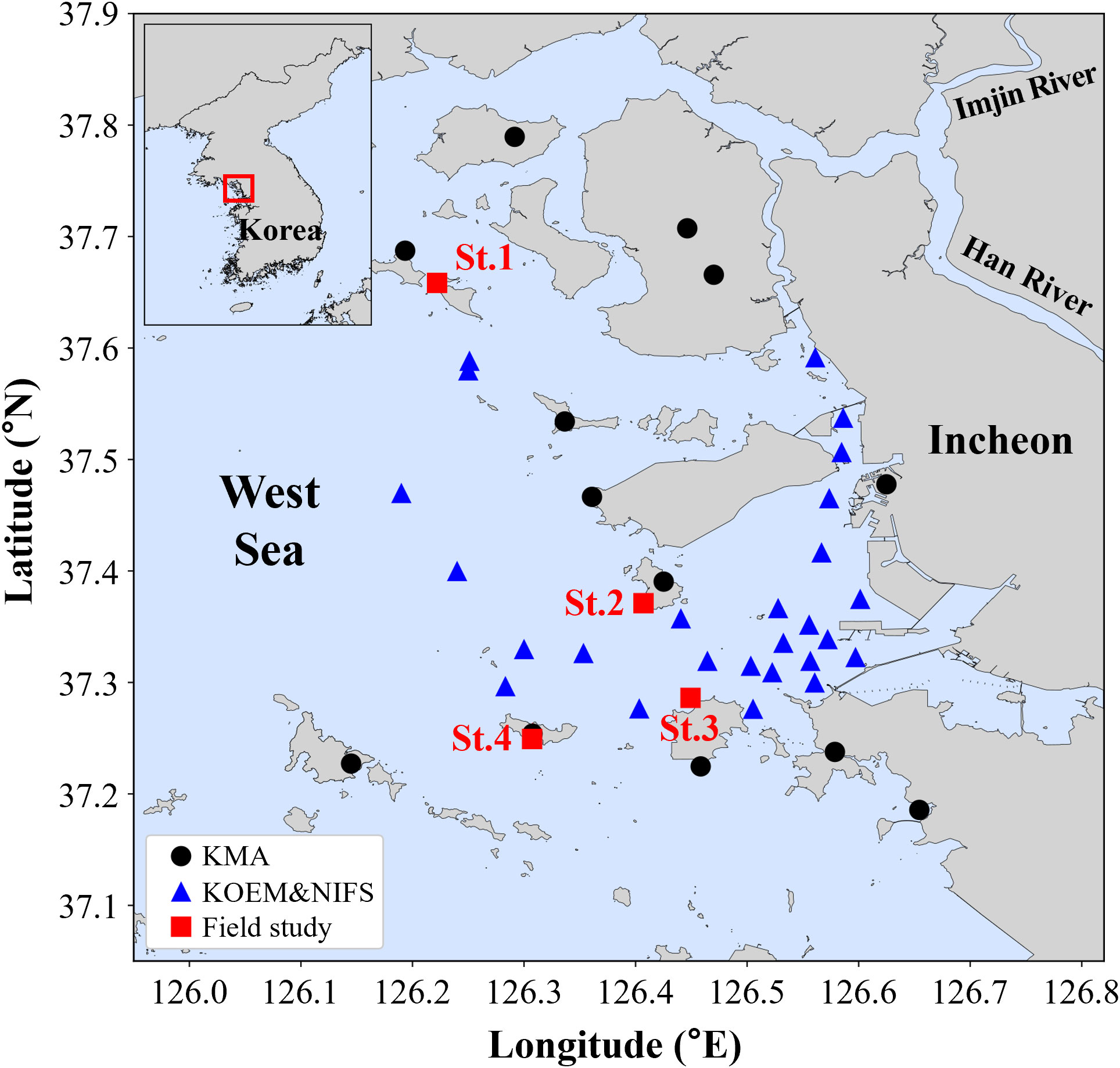
Figure 1 Study area and station locations in Incheon, South Korea. The black circles represent locations where data from the Korea Meteorological Administration (KMA) were collected. The blue triangles represent locations where data from the Korea Marine Environment Management Corporation (KOEM) and the National Institute of Fisheries Science (NIFS) were collected. The red rectangles represent the stations where field observations of oyster habitat were conducted.
Statistics on Korean fishery production consist of sales volume through the National Federation of Fisheries Cooperatives and non-systematic sales volume, which is sold directly by individuals without going through the national cooperative system. However, non-systematic sales volume has a higher level of uncertainty because the statistical survey targets random individuals, which reduces accuracy. Hence, in this study, only systematic statistical data were used to analyze oyster production. Monthly oyster production data for Incheon were obtained from the fishery production surveys of Statistics Korea (https://kosis.kr/). Oysters are harvested mainly in fall and winter (Lim et al., 2014; Hwang et al., 2016), so to calculate the annual production, the sum of monthly production from March of the current year to February of the following year was set as the annual production.
PCA is a dimensional reduction technique that projects variables onto axes (principal components) while preserving the maximum variance. Principal components are defined as the axes that maximize the variance, with the first principal component having the greatest variance. The reliability of each component is expressed as explainability; the higher the explainability of the principal component, the better it reflects the characteristics of multiple variables. The extent to which elements are projected onto the same principal component is the principal component coefficient; if these coefficients are similar, they are considered to be related elements. The PCA package (‘FactoMiner’ ver. 2.6) in R software (ver. 4.2.1; R studio: ver. 2022.07.2 + 576) was used to analyze seasonal observation data to identify correlations between each environmental factor and oyster production. Before proceeding with PCA, the variables were z-scored to remove scale differences between them.
The use of probabilistic statistical methods, such as Bayesian Network (BN) analysis, to analyze complex marine ecosystem models is increasing (Barton et al., 2008; Fiechter et al., 2013; McDonald et al., 2016). A BN is a graphical model that can intuitively represent the probabilistic structure of multivariate data using graphs and is used to measure how well a data dependency structure (causal relationship) is reflected (Pavlovic, 1999; Korb and Nicholson, 2010). A directed acyclic graph (DAG) is used to represent the uncertainty and probabilities of the relationships between variables. The graph consists of nodes pertaining to numerous variables and edges that represent the dependencies between variables and the causal relationships between nodes are expressed as probability information. This probability information can be understood using Bayes’ theorem, which expresses the relationship between the prior and posterior probabilities for events A and B as shown in Eq. (1),
where P(A) represents the prior probability of event A, P(B/A) represents the likelihood function that indicates the probability of event B occurring given the occurrence of event A, and P(A/B) represents the posterior probability that indicates the probability of event A occurring given that event B has occurred. According to Bayes’ theorem, P(A/B) is proportional to the product of the prior probability and likelihood function.
The BN structure is constructed primarily through structural learning or expert opinion. Structural learning is a method for directly studying the structure of a BN from data that represents the optimal relationships between variables, enabling a more objective construction of the network. However, as the number of variables increases, the number of possible network structures also increases exponentially, causing difficulties in deriving the optimal structure. Furthermore, although several structures may fit the data well, they may not be suitable for new data because of the possibilities of overfitting (Koller and Friedman, 2009). Therefore, with sufficient prior knowledge and expert opinions, a higher probability of accurate prediction can be achieved by setting a structure based on the causal relationships between variables. Hence in this study, factors affecting oyster production were selected based on a literature review and expert opinions, including AT, ST, salinity, DIN, DIP, Chl–a, and DOS.
We used a model-averaging technique to calculate the strength of the causal relationships between the variables in the BN model. Using this technique, we first generated multiple input datasets through bootstrapping and calculated the parameters by inputting them into the BN model. We then evaluated the performance and calculated the optimal connection structure using the model parameters obtained from each bootstrap model. We repeated this process several times and averaged the connection status between the nodes of each connection structure in the optimal BN model to express the probability of causal relationships as a ‘strength’. In this study, we performed BN analysis using the ‘bnlearn’ package (ver. 4.8.1) provided in R and analyzed the causal relationships between marine environmental factors and oyster production to identify the environmental factors that affect oyster production.
A field study was conducted at four stations in Incheon, including the stations where oyster mass mortality occurred at St.1 and St.4 (Figure 1). To investigate the effects of temperature on the habitat environment of oysters, thermometers (HOBO water Temp Pro v2) were installed in each station, and the temperature (accuracy ±0.21°C) was observed at 5-min intervals during summer (June–August) of 2020–2021. Additionally, the time of exposure to tidal emersion was calculated. Because of the geographical characteristics, the level of emersion was different in each area; hence, to ensure the accuracy of the distinction between exposed and non-exposed areas, the elevation levels (EL) of each station were measured using GPS and the standard levels for tidal height were determined for each station. The standard levels for tidal height were calculated by adding the mean sea level (MSL) to the EL at the thermometer locations.
Multiple stress tests of ST-salinity and AT-exposure time were performed to identify the tolerance range of oysters to environmental factors. As the size of yearling oysters in the study area was found to be 7 cm (Jeon et al., 2012), oysters measuring less than 7 cm were gathered in the vicinity of the study area to guarantee the use of oysters under one year old. The samples were then transported to the laboratory to maintain habitable temperatures. Filtered seawater from the natural habitat of the oysters was used as the culture water. The oysters were acclimated to the culture water in the laboratory for 3–4 weeks at a temperature of 21 ± 1°C and salinity of 28 ± 1 psu until the assay was conducted.
To determine the tolerance range of the submerged oysters to ST and salinity, we conducted multiple stress tests for ST-salinity. Prior to commencing the test, we ran single stress tests for each factor as a pre-test and set the range of environmental exposure for the multiple stress test (Table 1). The ST range for the multiple stress test was set at 1°C intervals between 25°C (the highest temperature with no effect in the single stress test) and 30°C (the lowest temperature with an adverse effect in the single stress test). The salinity range for this test was set at two levels; 25 psu, which was determined as the optimal salinity in the single stress test, and 28 psu, the average salinity of the Incheon coastal region in summer. The test was conducted over 40 days.
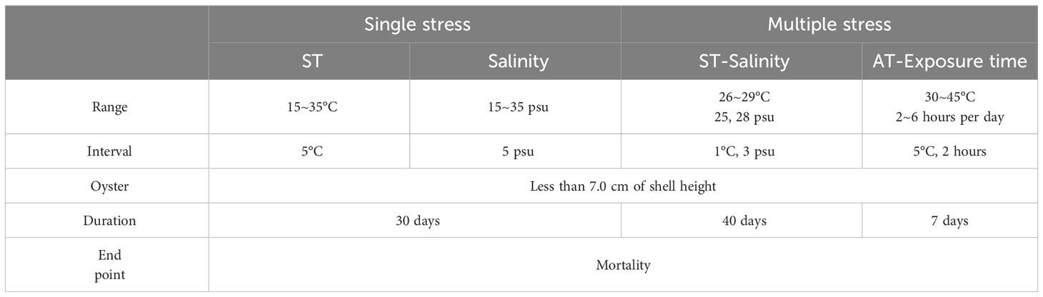
Table 1 Test conditions for identifying the environmental tolerance range of oysters.
Assuming that oysters would be exposed to air owing to the difference in tidal heights, we determined the tolerance range for AT and exposure time using a multiple-stress test (Table 1). The AT range was based on observation, starting from a temperature of 30°C, exceeding the highest ST in summer, and increasing in 5°C intervals up to 45°C, which is close to the highest AT. The exposure times were also based on observations and included 2, 4, and 6 hours per day. The test was conducted over 7 days.
Forty oysters were used per experimental condition (four replicates of 10 individuals each). Each condition was cultured in 50 L plastic aquariums, with 100% water change three times per week. Culture water was preconditioned to mitigate temperature shocks during water changes and the culture water in the tanks was continuously circulated internally using a circulating water thermostat. For air exposure conditions, all times outside the exposure period were incubated in the aquariums. The aquaria were provided with an aeration system, and water temperature, dissolved oxygen, and salinity were measured once daily. In addition, all individuals were cultured under identical conditions with no variation in culture water, food, temperature, or oxygen, except for the stimulus condition.
Survival rate was considered the primary endpoint of the tests and mortality was determined as individuals that opened the valves but failed to respond to external stimuli. One-way analysis of variance (ANOVA) was employed to assess the significance of survival rates under each stress condition. P values below 0.05 were deemed statistically significant.
Several environmental features of Incheon showed significant seasonal variation (Figure 2). AT and ST displayed a generalized pattern of values that were high in summer and low in winter (Figures 2A, B). In contrast, salinity tended to be low during the summer (Figure 2C), because of the inflow of freshwater through the Han River estuary during the East Asian monsoon (Yoon and Woo, 2015). DOS was relatively higher in spring and winter than in summer and fall but remained close to saturation due to active surface air exchange (Figure 2D). DIN was the lowest in spring and relatively high in winter (Figure 2E). The higher concentrations are likely due to increased physical mixing in winter, which supplies nutrients from deeper waters. DIP was relatively high in summer (Figure 2F), because of increased freshwater inflow from estuaries (Park et al., 2004). Chl-a, on the other hand, did not show significant seasonal variability and remained steady at 2–4 mg/L (Figure 2G).
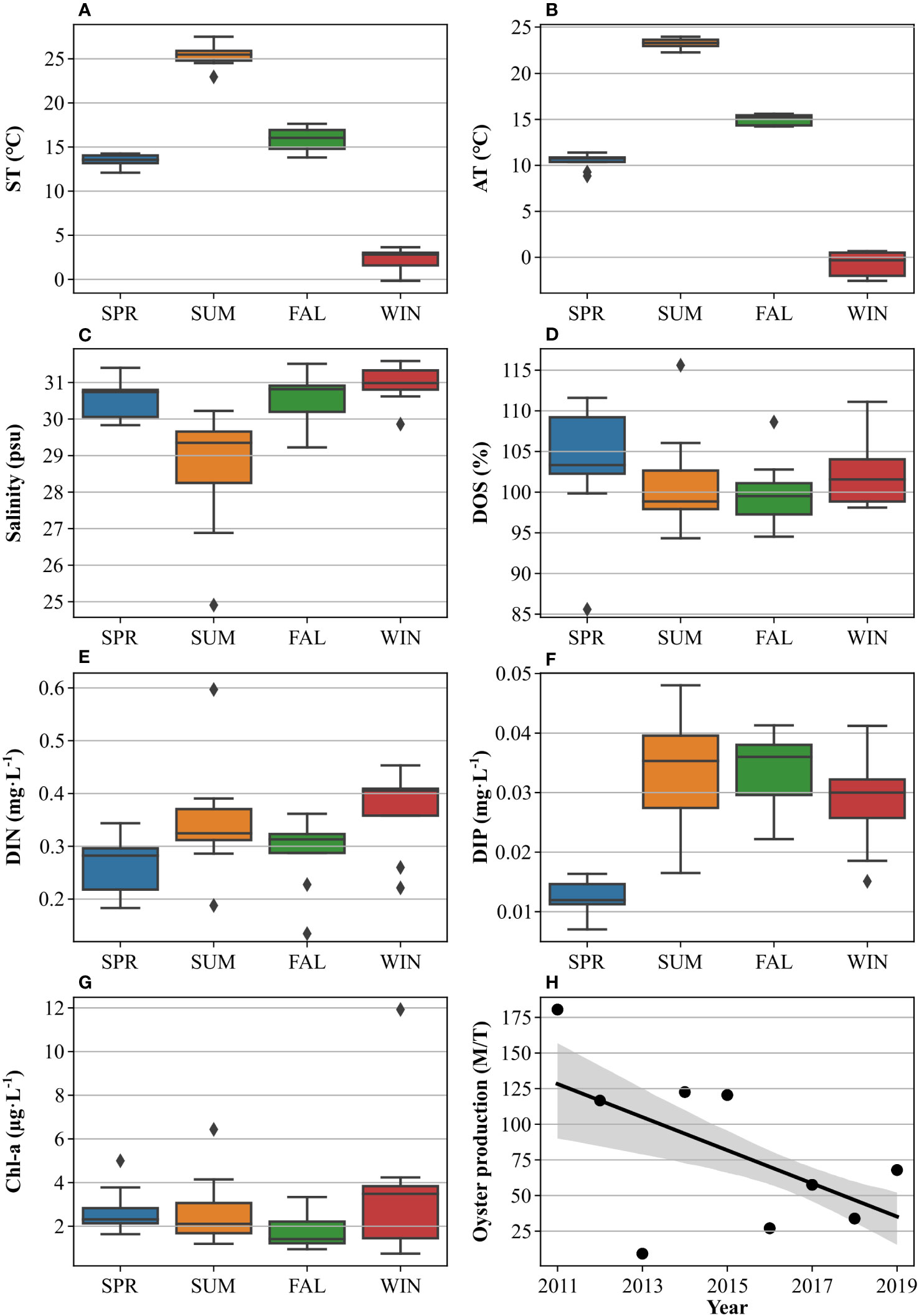
Figure 2 Seasonal distribution of ST (A), AT (B), salinity (C), DOS (D), DIN (E), DIP (F), and Chl-a (G), and annual oyster production (H) in Incheon from 2011 to 2019. The seasons were defined as SPR (spring), SUM (summer), FAL (Fall), and WIN (winter). For the oyster production, the black solid line represents the trend line, and the grey shaded area represents the 95% confidence level.
Generally, oysters in the western coast of Korea begin to breed and spawn in June when the sea temperature reaches 22–25°C, and are harvested from late fall (Lim et al., 2014; Hwang et al., 2016), with oyster production concentrated in fall and winter (Supplementary Table S1). While oyster production showed significant annual variability during the survey period, the overall production trend continually tended to decrease (-11.6 M/T/yr, p< 0.001) (Figure 2H).
PCA was performed to identify correlations between environmental factors and oyster production. The PCA results showed that the first and second principal components accounted for 34.2% and 25.2% of the total variances, respectively, with a cumulative proportion of 59.4% (Figure 3A). Regarding oyster production, the second principal component coefficient showed to be clearer with a value of -0.85 compared to the first principal coefficient which displayed a value of 0.17 (Figure 3B). Negative or low coefficients of the second principal component for other variances indicated a strong positive (+) correlation with oyster production, whereas positive or high coefficients indicated a strong negative (-) correlation.
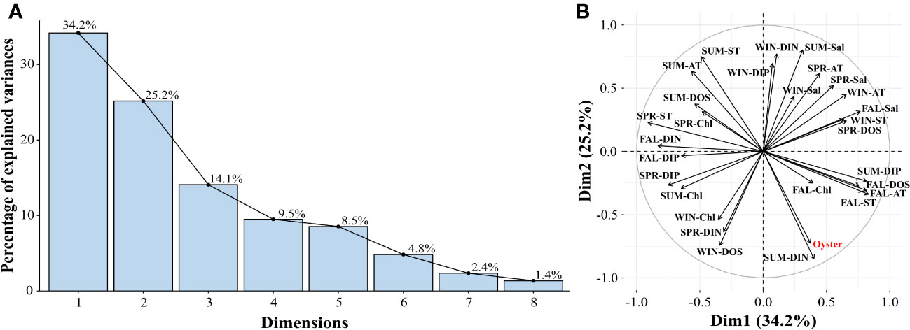
Figure 3 Percentage of explained variances (A) and biplot (B) according to the principal component analysis (PCA). The explained variances for the first 2 dimensions cover 59.4% of the variances.
In spring, ST showed a weak, negative correlation with oyster production, with a principal component coefficient of 0.33 (Figure 3B). DIP also showed a weak negative correlation, with a coefficient value of -0.38. AT, salinity, and Chl-a also showed a negative correlation with oyster production; however, this correlation was not strong enough to explain the overall variation, with a coefficient of 0.3 or less. In summer, most of the environmental features, except for Chl-a, explained the variability in oyster production. AT, ST, salinity, and DOS showed a strong negative correlation (principal component coefficients: 0.58–0.82) with oyster production, while DIN and DIP showed a strong positive correlation (principal component coefficient: -0.80–0.57) (Figure 3B). In fall, ST, DOS, and Chl-a showed a weak positive correlation (principal component coefficient: -0.39–0.31) with oyster production, while salinity showed a weak negative correlation (Figure 3B). AT and DIP were positively correlated with oyster production; however, the coefficients were low. DIN did not correlate with oyster production. In winter, DOS and Chl-a displayed a strong positive correlation (principal component coefficient -0.78 and -0.80, respectively) with oyster production, while DIN and DIP showed a strong negative correlation (principal component coefficient 0.70 and 0.78, respectively) (Figure 3B).
Based on the PCA results, AT, ST, salinity, DIN, DIP, Chl-a, and DOS were set as factors for use in the BN analysis. Because the oyster life cycle depends on seasonal environmental changes, individual factors were applied according to the season. In addition, to prevent the formation of dependent structures among different seasonal factors or factors with no relationship, a blacklist was applied before learning the model data. This blacklist was written based on the results of PCA and prior knowledge (Figure 4A).
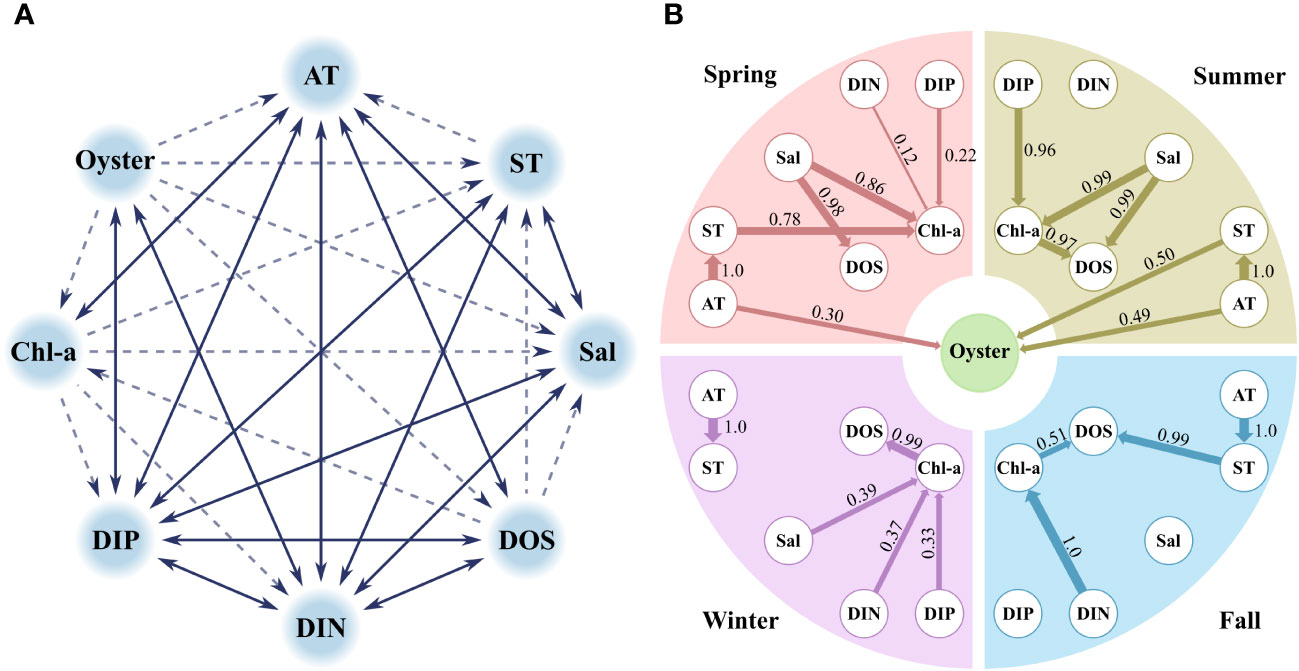
Figure 4 (A) Blacklist reflected before learning the data for the Bayesian network model and (B) results of the Bayesian network model. In this blacklist, the solid lines represent the prohibition of forming relationships in both directions, and the dashed lines represent the direction for the prohibition of forming relationships.
The BN results in the spring showed that AT was strongly dependent on ST, and ST was sequentially connected to Chl-a with a strength of 0.78 (Figure 4B). Salinity formed dependent structures with DOS and Chl-a, with strengths of 0.98 and 0.86, respectively, and DIN and DIP were weakly connected to Chl-a, with strengths of 0.12 and 0.22, respectively. In spring, AT displayed a causal relationship with oyster production with a strength of 0.30.
In the summer, salinity was strongly related to Chl-a and DOS, and DIP was strongly related to Chl-a with a strength of 0.96 (Figure 4B). Chl-a was also associated with DOS, with a strength of 0.97. DIN did not form structures dependent on other environmental factors. AT not only formed dependent structures with ST but also directly with oyster production with a strength of 0.49. In addition, ST showed a correlation with oyster production with a strength of 0.50.
In the fall, strong vertical structures formed from AT to ST and then to DOS (Figure 4B). DIN also formed a vertical structure that continued from Chl-a to DOS; however, this structure was weaker than that of AT and ST. Salinity and DIP did not form structures with any other factors and did not show any association with oyster production.
In the winter, AT formed a relationship with ST and did not form further structures (Figure 4B). Salinity, DIN, and DIP formed dependent structures with Chl-a, with strengths of 0.39, 0.37, and 0.33, respectively, and Chl-a displayed a strong structure with DOS. In winter, there was no relationships between oyster production and the other factors.
To investigate the effects of temperature on oyster, temperature observations were conducted in the emersion and immersion areas. The temperature difference (emersion temperature - immersion temperature) was particularly significant when the tidal difference was greater and the standard level for tidal height was higher. The mean emersion time in St.1 and St.4, which had higher standard levels (Table 2), were 3.6 ± 0.8 hours and 2.7 ± 1.2 hours, respectively, and the mean emersion time in St.2 and St.3, which had lower standard levels, were 1.5 ± 1.1 hours and 1.9 ± 1.2 hours, respectively. As the standard level increased, the emersion time increased; as a result, prolonged exposure to heat and solar radiation caused an increase in the emersion temperature. Indeed, the temperature tended to be higher during emersion at St.1 (Figure 5).
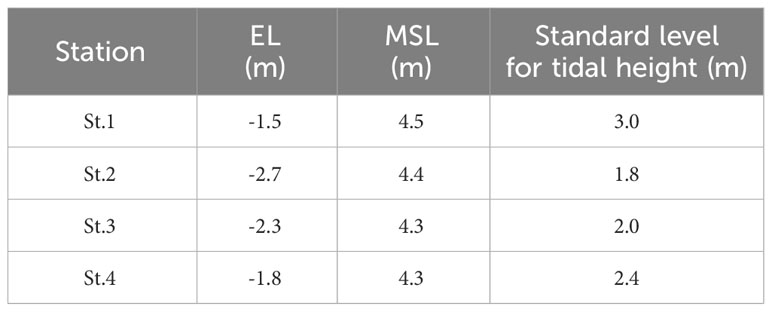
Table 2 Standard levels for tidal height calculated using elevation levels (EL) and mean sea levels (MSL).
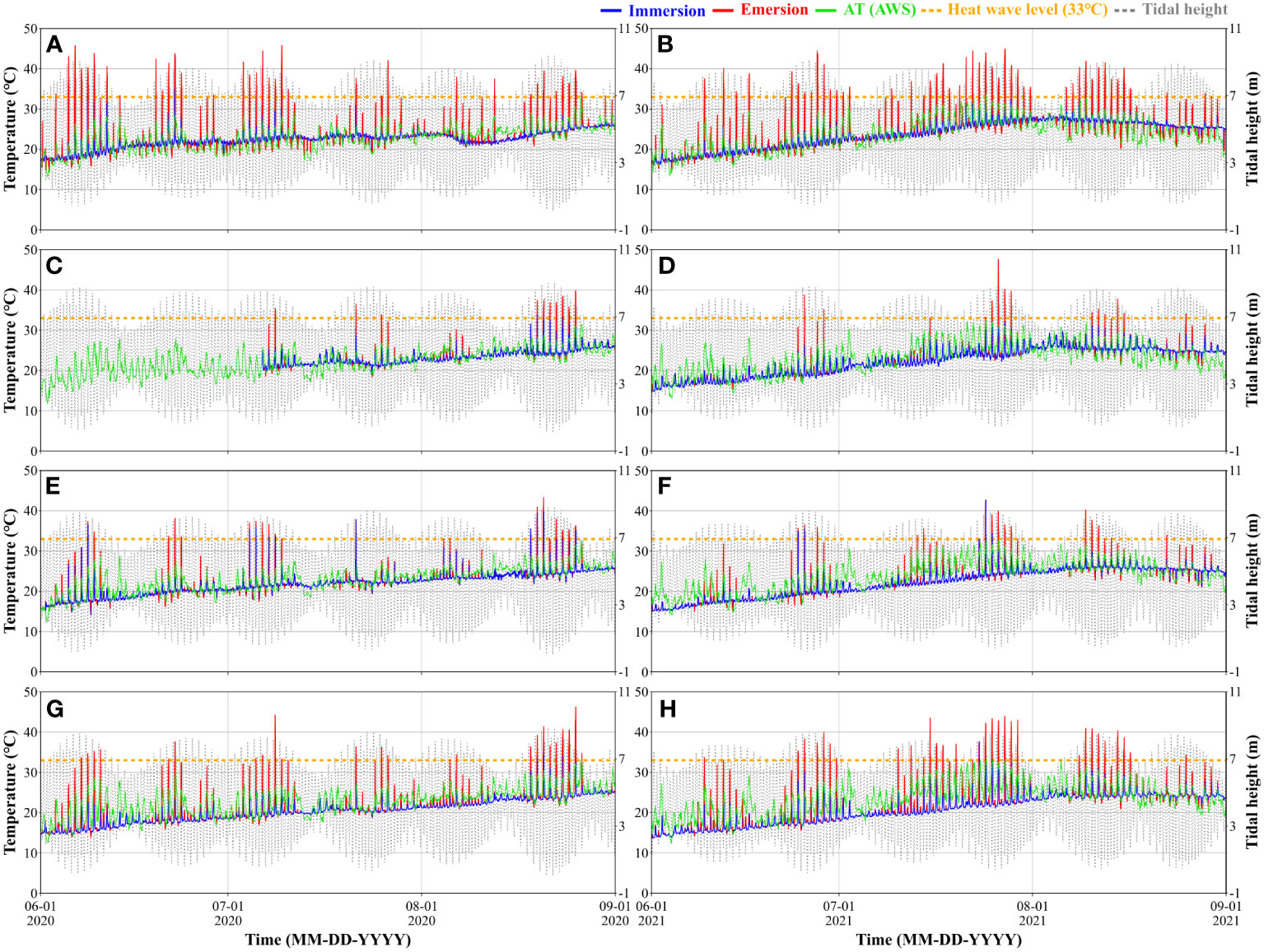
Figure 5 Temperature of oyster habitats continuously observed at St.1 (A, B), St.2 (C, D), St.3 (E, F), and St.4 (G, H) during the summer of 2020 and 2021. The standard levels for tidal height were used to distinguish the states of the oyster habitats into immersion (blue solid line) and emersion (red solid line) when the temperature was observed. The green solid lines represent the temperature observed at the nearest AWS to each station. The yellow dotted line represents the criterion for heat waves.
The number of days with heat waves (> 33°C) was the highest in St.1 (13.8 ± 3.8 days) and the lowest in St.2 (4.8 ± 2.2 days; Figures 5A–D). The duration of heat waves was the highest in St.1 (1.9 ± 0.2 hours) and lowest in St.2 (0.8 ± 0.6 hours). The highest number of consecutive heat wave days was observed at St.1 in July 2021, at 12 days, while the shortest number of consecutive days was observed at St.2 in August 2020, at 7 days. The mean temperature during heat waves showed a distribution of 34.7~35.4°C in all stations, with a maximum of 47.6°C observed.
In all stations, the mean number of days with heat waves increased by 9.6% from 8.3 ± 3.2 days in 2020 to 9.1 ± 5.5 days in 2021 (Figure 5). The mean number of consecutive days also increased by 9.6% from 5.2 ± 2.6 days in 2020 to 5.7 ± 3.5 days in 2021. The mean duration of extreme high temperature increased from 35.3 ± 1.0°C in 2020 to 35.6 ± 0.8°C in 2021, indicating that heat waves occurred more frequently and for longer periods in 2021 compared to 2020.
The BN result revealed no relationship between oyster production and salinity. This is inconsistent with the fact that salinity is a major factor affecting the oyster ecology. However, it is worth noting that although our data covered nine years, they were seasonal observations and not continuous observations. Thus, our data represent a snapshot of the environment and may not fully reflect the relationships between oysters and environmental factors. Our study area is located near estuaries influenced by the Han and Imjin rivers, and salinity is relatively low in summer when the monsoon occurs. To compensate for the limitations of our data, we conducted a laboratory study that included a salinity stress test in addition to ST.
Single- and multiple-stress tests for ST and salinity were conducted to understand the tolerance range of oysters to ST and salinity when submerged in seawater. In the single stress test for ST, survival rates over 95% were observed below 25°C, which rapidly decreased at temperature above 30°C (P value from 25–30°C:< 0.001), with all individuals dying at 35°C (P value between 30°C and 35°C:< 0.05) (Figure 6A and Supplementary Table S2). The results suggest a significant impact on the survival of oysters in ST exceeding 25°C. In the single stress test for salinity, survival rates were the highest at 25 psu and there was no significant difference in survival rates between 15–20 psu (P > 0.05) and 30–35 psu (P > 0.05) (Figure 6B and Supplementary Table S2). This suggests that oyster survival is greatest within the contiguous salinity range, including 25 psu, and that both lower and higher salinity levels adversely affect oyster survival.
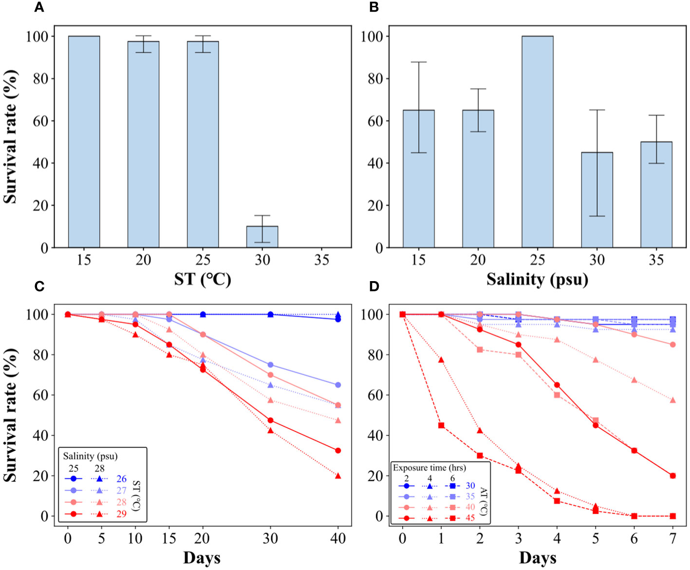
Figure 6 Survival rates of oysters for single stress tests on ST (A) and salinity (B). Survival rates of oysters for multiple stress tests on ST–salinity (C) and AT–exposure time (D).
The multiple stress test, based on the results of the single stress test, set the ST range at 26~29°C, which included the highest temperature (approximately 29°C in Figure 5) in summer. The salinity was divided into 25 psu, which was considered the optimal salinity range, and 28 psu, which was applied during the acclimation. At 26°C, there was no effect on mortality, however, the survival rates began to decrease from 27°C (P< 0.05) (Figure 6C; Table 3). The survival of oysters declined as ST increased and reached its minimum at 29°C and 28 psu after 40 days, with a survival rate of approximately 20%. The survival rates were lower in the 28 psu conditions compared to the 25 psu conditions across all ST conditions except 26°C, however, the observed differences with salinity in each ST condition were not statistically significant (Table 3). Between day 15 and day 20, we observed a significant decrease in survival rates for the 27 and 28°C conditions (P value:< 0.05) (Supplementary Table S3). Additionally, a significant decrease in survival rates for the 29°C condition was observed (P value:< 0.05) from day 10 (Supplementary Table S3).

Table 3 ANOVA P value for the survival rate of the multiple stress test on ST–salinity.
To determine the tolerance range of the oysters to AT and exposure time, a multiple stress test was conducted under the assumption that periods of low tide would affect such factors (Figure 6D). At an AT of 30°C, the survival rates of oysters were over 97.5%, even at an exposure time of 6 hours. Similarly, at temperatures of 35°C, all exposure times showed survival rates over 92.5%, indicating that air exposure had minimal effect on survival rate. At 40°C, when exposed for 4 hours, the survival rates of oysters decreased sharply to 57.5% (P< 0.05), and when exposed for 6 hours, it reached 20.0% (P< 0.05) (Table 4). In the 40°C and 6 hours exposure condition, mortality began from day 2 (P< 0.05) (Supplementary Table S4), and the survival rate fell below 40% at day 6. In the 45°C and 2 hours exposure, the survival rate was over 85.0% up to day 3, however, this decreased sharply to 20.0% at day 7. In the 45°C and 4 hours and 6 hours exposure, the survival rates of oysters significantly decreased from day 1 (P< 0.05), and reached zero at day 6 (Figure 6D; Supplementary Table S4).
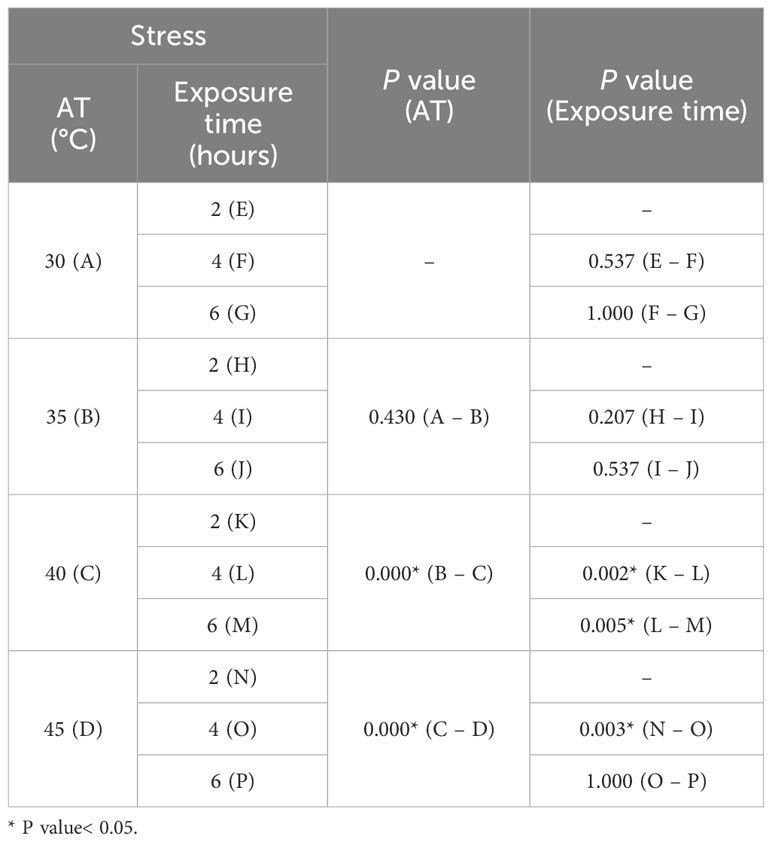
Table 4 ANOVA P value for the survival rate of the multiple stress test on AT–Exposure time.
When the results of the PCA and BN were combined, AT in spring and AT and ST in summer were related to oyster production. The surrounding environment was identified through field observations and its effects of the surrounding environment on oyster mortality were confirmed through stress tests. In the multiple stress test for ST and salinity, the mortality increased dramatically from 27°C and the survival rates were lower at 28 psu than at 25 psu. However, the ANOVA for exposure to salinity did not show a significant difference, making it difficult to conclude that mortality increased due to the difference in salinity (Table 3). Based on the results of calculating the P-values of survival rates under the same temperature conditions, ST was the primary factor affecting the survival rate of oysters. Furthermore, the survival rates of oysters decreased more quickly at 29°C than at 27–28°C, suggesting that the overall harm to oysters intensifies as the temperature rises.
The growth and mortality of oysters vary greatly depending on changes in environmental factors; in particular, temperature and salinity are thought to directly or indirectly affect maturity, feeding activity, metabolic reactions, and energy balance (Newell et al., 1977; Delaporte et al., 2006; Lee et al., 2018). In the Embryo-larval development stage, the effects of environmental factors on growth are understood through the occurrence rate of abnormal embryos and D-type embryos, and specific ranges of temperature (22–28°C) and salinity (22–33 psu) have been reported as the optimal growth range (Gamain et al., 2016; Gamain et al., 2017; Moreira et al., 2018a; Moreira et al., 2018b). In the larvae stage, the optimal condition is shown as the temperature range of 23–30°C and salinity range of 20–35 psu to enhance the growth of the shell height (His et al., 1989; Hofmann et al., 2004; Kheder et al., 2010; Han and Li, 2018). In the adult stage, optimal range is reported as temperatures of 15–25°C and salinity of 18–30 psu (Muranaka and Lannan, 1984; Gagnaire et al., 2006; Yang et al., 2016). Previous studies have shown results similar to the present results of ST and salinity tests.
Consistent findings have indicated a causative link between high ST and oyster mass mortality. Oxidative and nitrative stress in oysters are induced by elevated ST, which inhibit the antioxidant defense system (Rahman and Rahman, 2021). High temperatures reduce the number of hemocytes (Gagnaire et al., 2006; Rybovich et al., 2016). High temperatures can also cause a decline in reproductive function and have been found to reduce ovarian function in oysters by decreasing egg quantity and size, inducing cell death, and increasing the levels of reactive nitrogen and oxygen species (Nash et al., 2019). Moreover, high temperatures can cause severe damage to larvae and juveniles, which are less able to tolerate high temperatures than adults (Hofmann et al., 2004; Rybovich et al., 2016). The cumulative impact of elevated temperatures on immature stages and lower reproductive function in mature individuals may affect subsequent populations, resulting in decreased productivity.
Oysters that live in the intertidal zone are inevitably exposed to air for several hours daily. The difference in temperature between air and seawater caused by tides causes a drastic change in the thermal environment around the oyster habitat, which is particularly severe during the summer. In the field observation, high temperatures of 34.7–35.4°C (maximum 47.6°C) were observed for average durations of 0.8–1.9 hours (maximum 3.6 hours). Furthermore, heat waves occurred for a maximum of 12 consecutive days. Results from the multiple stress test showed that when exposed to 40°C and 4 hours, the survival rate of oysters decreased dramatically to 57.5% after 7 days, and when exposed to 45°C and 4 hours, the survival rate was 42.5% after only 2 days, and zero after 6 days. When the results from the field observation and stress test were combined, it could be inferred that high temperatures during emersion were one of the cause for mass mortality of oysters in summer, and in particular, prolonged exposure increased the mortality rate due to heat stress.
The range of air exposure tolerance in oysters is not well known; however, air exposure during emersion can cause rapid temperature changes, dehydration, hypoxia, and acidification in the bodies of aquatic organisms (Shpigel et al., 1992; Morash and Alter, 2016). When oysters are exposed to air, they close their valves to block gas exchange (Willson and Burnett, 2000). Allen and Burnett (2008) reported that the interruption of oxygen supply due to closed valves causes oxygen depletion and accumulation of carbon dioxide in the hemolymph which ultimately leads to a decrease in pH. Additionally, they found that temperature increases reduce the oyster’s immune system, with the bactericidal index of hemolymph against Vibrio campbellii greatly decreasing at 30°C. Although the survival rate did not decrease at 30°C in the exposure stress test of the present study, the present test was conducted in a controlled environment. In an uncontrolled natural environment, exposure to air in summer may have a greater impact on oyster mortality.
Exposure to heat waves has varying effects on intertidal bivalves, and the study of Manila clams provides valuable insights. In simulated scenarios at 50°C and only two days of air exposure, Manila clams were highly vulnerable to atmospheric heat waves, resulting in 100% mortality (He et al., 2022b). As the study progressed, the clams exhibited significantly increased enzymatic activity, particularly when repeatedly exposed to heat waves. Clams respond to heat waves by increasing their metabolic rate and stimulating specific enzymes and genes, at the expense of physiological maintenance (He et al., 2022a).
Although oysters are highly adaptable to harsh environments (i.e., intertidal zone) and possess a wide range of environmental stress resistance (Zhang et al., 2012), they are vulnerable to heat stress caused by high temperatures (Kawabe et al., 2010; Rybovich et al., 2016). Based on the results of this study, we argue that an increase in heat energy due to climate change could have a negative impact on oyster survival. Regardless of greenhouse gas emission scenarios, a temperature increase of 1.5°C by 2040 is almost inevitable (Masson-Delmotte et al., 2021) and the related increase in thermal stress may have a negative impact on oyster survival. Sea and air temperatures have been rising continuously in Incheon and oyster production has been declining steadily (Figure 7). Despite the decline in oyster production, it is unlikely to cease in the near future. However, the negative correlation between the temperature and oyster production should not be ignored. Furthermore, stronger heat waves are predicted to occur more frequently by 2051–2080 and record-breaking heat waves that surpass previous records are predicted to occur every 9-37 years in the mid-latitudes of the Northern Hemisphere (Fischer et al., 2021). Given that a significant number of oysters inhabit the mid-latitudes of the Northern Hemisphere (Beck et al., 2011), these record-breaking heat waves can cause irreversible changes in oyster habitats.
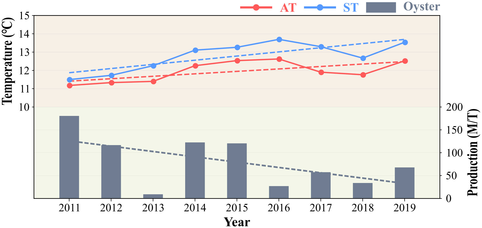
Figure 7 Annual mean AT (red solid line) and ST (blue solid line), and annual oyster production (bar plot) from 2011 to 2019. The dotted lines represent the trend lines of each parameter.
Oyster production in Incheon is continuously decreasing because of mass mortality in the summer. To identify the cause of such mortality, the relationship between the environment and oyster production was identified through PCA and BN analyses. The results showed that air temperatures in spring and air and sea temperatures in summer were related to the survival rate of oysters. Through field observations, the environment exposed to oysters during emersion and immersion was identified and environmental stress tests were conducted based on these findings. Stress tests showed that the survival rate of oysters increased inversely with exposure time and temperature. Hence, these results indicate the possibility of exposure to high temperatures as a cause of mass mortality in summer. Recent climate change patterns have made the outlook for oyster production more pessimistic. In addition to simple temperature increases, more intense and frequent heat waves can have fatal effects on oyster mass mortality. To understand the effects of future thermal stress on oysters more accurately, long-term trend analyses and field-based observations must be conducted simultaneously.
The datasets presented in this study can be found in online repositories. The datasets of the KMA can be found below: https://data.kma.go.kr/. The datasets of the KOEM can be found below: https://meis.go.kr/. The datasets of the NIFS can be found below: https://www.nifs.go.kr/kodc/index.kodc/. The datasets of the Statistics Korea can be found below: https://kosis.kr/.
JH: Writing – original draft, Writing – review & editing. SK: Writing – original draft, Writing – review & editing. DK: Writing – review & editing. SL: Writing – review & editing. JL: Writing – review & editing. MK: Writing – review & editing. SK: Writing – original draft, Writing – review & editing.
The author(s) declare financial support was received for the research, authorship, and/or publication of this article. This research was supported by Korea Institute of Marine Science & Technology Promotion (KIMST) funded by the Ministry of Oceans and Fisheries (202300238486 and 202300239887). The funder was not involved in the study design, collection, analysis, interpretation of data, the writing of this article or the decision to submit it for publication.
Authors J-MH, S-SK, D-YK, SK was employed by the company ARA Consulting & Technology Ltd. Author SL was employed by the company E&C Technology Co. Ltd. Authors JL, MK wasemployed by the company NeoEnBiz Co.
All claims expressed in this article are solely those of the authors and do not necessarily represent those of their affiliated organizations, or those of the publisher, the editors and the reviewers. Any product that may be evaluated in this article, or claim that may be made by its manufacturer, is not guaranteed or endorsed by the publisher.
The Supplementary Material for this article can be found online at: https://www.frontiersin.org/articles/10.3389/fmars.2023.1275521/full#supplementary-material
Allen S. M., Burnett L. E. (2008). The effects of intertidal air exposure on the respiratory physiology and the killing activity of hemocytes in the pacific oyster, Crassostrea gigas (Thunberg). J. Exp. Mar. Bio. Ecol. 357, 165–171. doi: 10.1016/J.JEMBE.2008.01.013
Bahr L. M., Lanier W. P. (1981). The ecology of intertidal oyster reefs of the South Atlantic Coast: A community profile. Washington: Office of Biological Services.
Barton D. N., Saloranta T., Moe S. J., Eggestad H. O., Kuikka S. (2008). Bayesian belief networks as a meta-modelling tool in integrated river basin management — Pros and cons in evaluating nutrient abatement decisions under uncertainty in a Norwegian river basin. Ecol. Econ. 66, 91–104. doi: 10.1016/J.ECOLECON.2008.02.012
Beck M. W., Brumbaugh R. D., Airoldi L., Carranza A., Coen L. D., Crawford C., et al. (2011). Oyster reefs at risk and recommendations for conservation, restoration, and management. Bioscience 61, 107–116. doi: 10.1525/bio.2011.61.2.5
Berthelin C., Kellner K., Mathieu M. (2000). Storage metabolism in the Pacific oyster (Crassostrea gigas) in relation to summer mortalities and reproductive cycle (West Coast of France). Comp. Biochem. Physiol. Part B Biochem. Mol. Biol. 125, 359–369. doi: 10.1016/S0305-0491(99)00187-X
Breitburg D., Coen L., Luckenbach M., Mann R. L., Posey M., Wesson J. A. (2000). Oyster reef restoration: convergence of harvest and conservation strategies. J. Shellfish Res. 19, 371–377.
Brown J. R., Hartwick E. B. (1988). Influences of temperature, salinity and available food upon suspended culture of the Pacific oyster, Crassostrea gigas: II. Condition index and survival. Aquaculture 70, 253–267. doi: 10.1016/0044-8486(88)90100-7
Cassis D., Pearce C. M., Maldonado M. T. (2011). Effects of the environment and culture depth on growth and mortality in juvenile Pacific oysters in the Strait of Georgia, British Columbia. Aquac. Environ. Interact. 1, 259–274. doi: 10.3354/aei00025
Cheney D., MacDonald B. F., Elston R. A. (2000). Summer mortality of Pacific oysters, Crassostrea gigas (Thunberg): Initial findings on multiple environmental stressors in Puget Sound, Washington 1998. J. Shellfish Res. 18, 456–473.
Cho S. M., Jeon B. S., Park S. I., Yoon H. C. (2009). Geotextile Tube Application as the Cofferdam at the Foreshore with Large Tidal Range for Incheon Bridge Project BT - Geosynthetics in Civil and Environmental Engineering. Eds. Li G., Chen Y., Tang X. (Berlin, Heidelberg: Springer Berlin Heidelberg), 591–596. doi: 10.1007/978-3-540-69313-0_110
Choi H. J., Jeong T.-Y., Yoon H., Oh B. Y., Han Y. S., Hur M. J., et al. (2018). Comparative microbial communities in tidal flats sediment on Incheon, South Korea. J. Gen. Appl. Microbiol. 64, 232–239. doi: 10.2323/jgam.2017.12.007
Choi K.-S. (2008). “Oyster capture-based aquaculture in the Republic of Korea”, in Capture-based Aquaculture Global overview. (Rome: FAO), 271–286.
Clements J. C., Davidson J. D. P., McQuillan J. G., Comeau L. A. (2018). Increased mortality of harvested eastern oysters (Crassostrea virginica) is associated with air exposure and temperature during a spring fishery in Atlantic Canada. Fish. Res. 206, 27–34. doi: 10.1016/j.fishres.2018.04.022
Delaporte M., Soudant P., Lambert C., Moal J., Pouvreau S., Samain J. F. (2006). Impact of food availability on energy storage and defense related hemocyte parameters of the Pacific oyster Crassostrea gigas during an experimental reproductive cycle. Aquaculture 254, 571–582. doi: 10.1016/J.AQUACULTURE.2005.10.006
Fiechter J., Herbei R., Leeds W., Brown J., Milliff R., Wikle C., et al. (2013). A Bayesian parameter estimation method applied to a marine ecosystem model for the coastal Gulf of Alaska. Ecol. Modell. 258, 122–133. doi: 10.1016/J.ECOLMODEL.2013.03.003
Fischer E. M., Sippel S., Knutti R. (2021). Increasing probability of record-shattering climate extremes. Nat. Clim. Change 11, 689–695. doi: 10.1038/s41558-021-01092-9
Flores-Vergara C., Cordero-Esquivel B., Cerón-Ortiz A. N., Arredondo-Vega B. O. (2004). Combined effects of temperature and diet on growth and biochemical composition of the Pacific oyster Crassostrea gigas (Thunberg) spat. Aquac. Res. 35, 1131–1140. doi: 10.1111/j.1365-2109.2004.01136.x
Fodrie F. J., Rodriguez A. B., Gittman R. K., Grabowski J. H., Lindquist N. L., Peterson C. H., et al. (2017). Oyster reefs as carbon sources and sinks. Proc. R. Soc B Biol. Sci. 284, 20170891. doi: 10.1098/rspb.2017.0891
Gagnaire B., Frouin H., Moreau K., Thomas-Guyon H., Renault T. (2006). Effects of temperature and salinity on haemocyte activities of the Pacific oyster, Crassostrea gigas (Thunberg). Fish Shellfish Immunol. 20, 536–547. doi: 10.1016/j.fsi.2005.07.003
Gamain P., Gonzalez P., Cachot J., Clérandeau C., Mazzella N., Gourves P. Y., et al. (2017). Combined effects of temperature and copper and S-metolachlor on embryo-larval development of the Pacific oyster, Crassostrea gigas. Mar. pollut. Bull. 115, 201–210. doi: 10.1016/J.MARPOLBUL.2016.12.018
Gamain P., Gonzalez P., Cachot J., Pardon P., Tapie N., Gourves P. Y., et al. (2016). Combined effects of pollutants and salinity on embryo-larval development of the Pacific oyster, Crassostrea gigas. Mar. Environ. Res. 113, 31–38. doi: 10.1016/J.MARENVRES.2015.11.002
Gerritsen J., Holland A. F., Irvine D. E. (1994). Suspension-feeding bivalves and the fate of primary production: An estuarine model applied to Chesapeake Bay. Estuaries 17, 403–416. doi: 10.2307/1352673
Grabowski J. H., Peterson C. H. (2007). ““15 - restoring oyster reefs to recover ecosystem services,”,” in Ecosystem Engineers. Eds. Cuddington K., Byers J. E., Wilson W. G., Hastings A. B. T.-T. E. S. (Cambridge, Massachusetts: Academic Press), 281–298. doi: 10.1016/S1875-306X(07)80017-7
Han Z., Li Q. (2018). Different responses between orange variant and cultured population of the Pacific oyster Crassostrea gigas at early life stage to temperature-salinity combinations. Aquac. Res. 49, 2233–2239. doi: 10.1111/are.13680
He G., Peng Y., Liu X., Liu Y., Liang J., Xu X., et al. (2022a). Post-responses of intertidal bivalves to recurrent heatwaves. Mar. pollut. Bull. 184, 114223. doi: 10.1016/j.marpolbul.2022.114223
He G., Zou J., Liu X., Liang F., Liang J., Yang K., et al. (2022b). Assessing the impact of atmospheric heatwaves on intertidal clams. Sci. Total Environ. 841, 156744. doi: 10.1016/j.scitotenv.2022.156744
Herbert R. J. H., Humphreys J., Davies C. J., Roberts C., Fletcher S., Crowe T. P. (2016). Ecological impacts of non-native Pacific oysters (Crassostrea gigas) and management measures for protected areas in Europe. Biodivers. Conserv. 25, 2835–2865. doi: 10.1007/s10531-016-1209-4
His E., Robert R., Dinet A. (1989). Combined effects of temperature and salinity on fed and starved larvae of the Mediterranean mussel Mytilus galloprovincialis and the Japanese oyster Crassostrea gigas. Mar. Biol. 100, 455–463. doi: 10.1007/BF00394822
Hofmann E. E., Powell E. N., Bochenek E. A., Klinck J. M. (2004). A modelling study of the influence of environment and food supply on survival of Crassostrea gigas larvae. ICES J. Mar. Sci. 61, 596–616. doi: 10.1016/j.icesjms.2004.03.029
Hwang I. J., Han J. C., Hur Y. B., Lim H. J. (2016). Seasonal variation in the body composition, amino acid, fatty acid and glycogen contents of triploid Pacific oyster, Crassostrea gigas in western coastal waters of Korea. Korean J. Malacol. 32, 269–277. doi: 10.9710/kjm.2016.32.4.269
Jeon C.-Y., Hur Y.-B., Cho K.-C. (2012). The effect of water temperature and salinity on settlement of Pacific oyster, Crassostrea gigas pediveliger larvae. Korean J. Malacol. 28, 21–28. doi: 10.9710/kjm.2012.28.1.021
Jeung H.-D., Keshavmurthy S., Lim H.-J., Kim S.-K., Choi K.-S. (2016). Quantification of reproductive effort of the triploid Pacific oyster, Crassostrea gigas raised in intertidal rack and bag oyster culture system off the west coast of Korea during spawning season. Aquaculture 464, 374–380. doi: 10.1016/j.aquaculture.2016.07.010
Kawabe S., Takada M., Shibuya R., Yokoyama Y. (2010). Biochemical changes in oyster tissues and hemolymph during long-term air exposure. Fish. Sci. 76, 841–855. doi: 10.1007/s12562-010-0263-1
Kheder R.B., Moal J., Robert R. (2010). Impact of temperature on larval development and evolution of physiological indices in Crassostrea gigas. Aquaculture 309, 286–289. doi: 10.1016/J.AQUACULTURE.2010.09.005
Koh C.-H., Khim J. S. (2014). The Korean tidal flat of the Yellow Sea: Physical setting, ecosystem and management. Ocean Coast. Manage. 102, 398–414. doi: 10.1016/j.ocecoaman.2014.07.008
Koller D., Friedman N. (2009). Probabilistic Graphical Models: Principles and Techniques. (Cambridge, Massachusetts: MIT Press).
Korb K. B., Nicholson A. E. (2010). Bayesian Artificial Intelligence. (Boca Raton, Florida: CRC Press). doi: 10.1201/b10391
La Peyre J. F., Casas S. M., Supan J. E. (2018). Effects of controlled air exposure on the survival, growth, condition, pathogen loads and refrigerated shelf life of eastern oysters. Aquac. Res. 49, 19–29. doi: 10.1111/are.13427
Lee Y.-J., Han E., Wilberg M. J., Lee W. C., Choi K.-S., Kang C.-K. (2018). Physiological processes and gross energy budget of the submerged longline-cultured Pacific oyster Crassostrea gigas in a temperate bay of Korea. PloS One 13, e0199752. doi: 10.1371/journal.pone.0199752
Lim H. J., Lim M. S., Lee W. Y., Choi E. H., Yoon J. H., Park S. Y., et al. (2014). Condition index and hemocyte apoptosis as a health indicator for the Pacific oysters, Crassostrea gigas cultured in the western coastal waters of Korea. Korean J. Malacol. 30, 189–196. doi: 10.9710/kjm.2014.30.3.189
Malham S. K., Cotter E., O’Keeffe S., Lynch S., Culloty S. C., King J. W., et al. (2009). Summer mortality of the Pacific oyster, Crassostrea gigas, in the Irish Sea: The influence of temperature and nutrients on health and survival. Aquaculture 287, 128–138. doi: 10.1016/J.AQUACULTURE.2008.10.006
Masson-Delmotte V., Zhai P., Pirani A., Connors S. L., Péan C., Berger S., et al (Eds.) (2021). Climate Change 2021: The Physical Science Basis. Contribution of Working Group I to the Sixth Assessment Report of the Intergovernmental Panel on Climate Change. (Cambridge, United Kingdom: Cambridge University Press). doi: 10.1017/9781009157896
McDonald K. S., Tighe M., Ryder D. S. (2016). An ecological risk assessment for managing and predicting trophic shifts in estuarine ecosystems using a Bayesian network. Environ. Model. Software 85, 202–216. doi: 10.1016/J.ENVSOFT.2016.08.014
Morash A. J., Alter K. (2016). Effects of environmental and farm stress on abalone physiology: perspectives for abalone aquaculture in the face of global climate change. Rev. Aquac. 8, 342–368. doi: 10.1111/raq.12097
Moreira A., Figueira E., Libralato G., Soares A. M. V. M., Guida M., Freitas R. (2018a). Comparative sensitivity of Crassostrea angulata and Crassostrea gigas embryo-larval development to as under varying salinity and temperature. Mar. Environ. Res. 140, 135–144. doi: 10.1016/J.MARENVRES.2018.06.003
Moreira A., Freitas R., Figueira E., Volpi Ghirardini A., Soares A. M. V. M., Radaelli M., et al. (2018b). Combined effects of arsenic, salinity and temperature on Crassostrea gigas embryotoxicity. Ecotoxicol. Environ. Saf. 147, 251–259. doi: 10.1016/J.ECOENV.2017.08.043
Muranaka M. S., Lannan J. E. (1984). Broodstock management of Crassostrea gigas: Environmental influences on Broodstock conditioning. Aquaculture 39, 217–228. doi: 10.1016/0044-8486(84)90267-9
Nash S., Johnstone J., Rahman M. S. (2019). Elevated temperature attenuates ovarian functions and induces apoptosis and oxidative stress in the American oyster, Crassostrea virginica: potential mechanisms and signaling pathways. Cell Stress Chaperones 24, 957–967. doi: 10.1007/s12192-019-01023-w
Newell R. I. E., Cornwell J. C., Owens M. S. (2002). Influence of simulated bivalve biodeposition and microphytobenthos on sediment nitrogen dynamics: A laboratory study. Limnol. Oceanogr. 47, 1367–1379. doi: 10.4319/lo.2002.47.5.1367
Newell R. C., Johson L. G., Kofoed L. H. (1977). Adjustment of the components of energy balance in response to temperature change in Ostrea edulis. Oecologia 30, 97–110.
Newell R. I. E., Koch E. W. (2004). Modeling seagrass density and distribution in response to changes in turbidity stemming from bivalve filtration and seagrass sediment stabilization. Estuaries 27, 793–806. doi: 10.1007/BF02912041
Park Y. C., Lee H. J., Kim D. W., Lee M. Y. (2004). “Nutrient dynamics and short-time scale variability of environmental parameters during the tidal cycle in the coastal waters of Incheon, Korea,” in Oceans ‘04 MTS/IEEE Techno-Ocean ‘04 (IEEE Cat. No.04CH37600), vol. 3. (1281-1283). doi: 10.1109/OCEANS.2004.1405764
Pavlovic V. I. (1999). Dynamic Bayesian networks for information fusion withapplications to human-computer interfaces. Ph.D. thesis. Illinois: University of Illinois Urbana-Champaign.
Peterson C. H., Lipcius R. N. (2003). Conceptual progress towards predicting quantitative ecosystem benefits of ecological restorations. Mar. Ecol. Prog. Ser. 264, 297–307. doi: 10.3354/meps264297
Rahman M. S., Rahman M. S. (2021). Effects of elevated temperature on prooxidant-antioxidant homeostasis and redox status in the American oyster: Signaling pathways of cellular apoptosis during heat stress. Environ. Res. 196, 110428. doi: 10.1016/j.envres.2020.110428
Ruesink J. L., Lenihan H. S., Trimble A. C., Heiman K. W., Micheli F., Byers J. E., et al. (2005). Introduction of non-native oysters: ecosystem effects and restoration implications. Annu. Rev. Ecol. Evol. Syst. 36, 643–689. doi: 10.1146/annurev.ecolsys.36.102003.152638
Rybovich M., Peyre M. K., Hall S. G., La Peyre J. F. (2016). Increased temperatures combined with lowered salinities differentially impact oyster size class growth and mortality. J. Shellfish Res. 35, 101–113. doi: 10.2983/035.035.0112
Sehlinger T., Lowe M. R., La Peyre M. K., Soniat T. M. (2019). Differential effects of temperature and salinity on growth and mortality of oysters (Crassostrea virginica) in Barataria bay and Breton sound, Louisiana. J. Shellfish Res. 38, 317–326. doi: 10.2983/035.038.0212
Shpigel M., Barber B. J., Mann R. (1992). Effects of elevated temperature on growth, gametogenesis, physiology, and biochemical composition in diploid and triploid Pacific oysters, Crassostrea gigas Thunberg. J. Exp. Mar. Bio. Ecol. 161, 15–25. doi: 10.1016/0022-0981(92)90186-E
Willson L. L., Burnett L. E. (2000). Whole animal and gill tissue oxygen uptake in the Eastern oyster, Crassostrea virginica: Effects of hypoxia, hypercapnia, air exposure, and infection with the protozoan parasite Perkinsus marinus. J. Exp. Mar. Bio. Ecol. 246, 223–240. doi: 10.1016/S0022-0981(99)00183-5
Yang C. Y., Sierp M. T., Abbott C. A., Li Y., Qin J. G. (2016). Responses to thermal and salinity stress in wild and farmed Pacific oysters Crassostrea gigas. Comp. Biochem. Physiol. Part A Mol. Integr. Physiol. 201, 22–29. doi: 10.1016/J.CBPA.2016.06.024
Yoon B., Woo S.-B. (2015). The along-channel salinity distribution and its response to river discharge in tidally-dominated Han river estuary, South Korea. Proc. Eng. 116, 763–770. doi: 10.1016/j.proeng.2015.08.362
Zhang G., Fang X., Guo X., Li L., Luo R., Xu F., et al. (2012). The oyster genome reveals stress adaptation and complexity of shell formation. Nature 490, 49–54. doi: 10.1038/nature11413
Zhang Z., Li X., Vandepeer M., Zhao W. (2006). Effects of water temperature and air exposure on the lysosomal membrane stability of hemocytes in pacific oysters, Crassostrea gigas (Thunberg). Aquaculture 256, 502–509. doi: 10.1016/j.aquaculture.2006.02.003
Keywords: pacific oyster, mass mortality, Bayesian Network, machine learning, tidal emersion, heat wave, climate change
Citation: Heo J-M, Kim S-S, Kim D-Y, Lee SW, Lee JS, Kang MH and Kim SE (2023) Impact of exposure temperature rise on mass mortality of tidal flat pacific oysters. Front. Mar. Sci. 10:1275521. doi: 10.3389/fmars.2023.1275521
Received: 10 August 2023; Accepted: 20 October 2023;
Published: 02 November 2023.
Edited by:
Kwang-Sik Albert Choi, Jeju National University, Republic of KoreaReviewed by:
Hee Yoon Kang, Chonnam National University, Republic of KoreaCopyright © 2023 Heo, Kim, Kim, Lee, Lee, Kang and Kim. This is an open-access article distributed under the terms of the Creative Commons Attribution License (CC BY). The use, distribution or reproduction in other forums is permitted, provided the original author(s) and the copyright owner(s) are credited and that the original publication in this journal is cited, in accordance with accepted academic practice. No use, distribution or reproduction is permitted which does not comply with these terms.
*Correspondence: Seong Eun Kim, Z29kaGtpbUBuYXZlci5jb20=
Disclaimer: All claims expressed in this article are solely those of the authors and do not necessarily represent those of their affiliated organizations, or those of the publisher, the editors and the reviewers. Any product that may be evaluated in this article or claim that may be made by its manufacturer is not guaranteed or endorsed by the publisher.
Research integrity at Frontiers
Learn more about the work of our research integrity team to safeguard the quality of each article we publish.