 Samuel Bunson
 Chuanmin Hu
94% of researchers rate our articles as excellent or good
Learn more about the work of our research integrity team to safeguard the quality of each article we publish.
Find out more
REVIEW article
Front. Mar. Sci. , 11 December 2023
Sec. Ocean Observation
Volume 10 - 2023 | https://doi.org/10.3389/fmars.2023.1275445
Natural disasters such as earthquakes and/or tsunamis may cause disturbance to the ocean, which can possibly lead to changes in the ocean properties. Here, we review the literature for the reported pre- or post-event changes of such properties, which include chlorophyll-a concentration, temperature, and turbidity in the surface ocean. Most of the reported changes were based on remotely sensed ocean properties, and such changes were attributed to the ocean’s response to the events. Here, by using the same remote sensing data collected in non-event years as the ‘control’ experiments or by analyzing the same remote sensing data at different spatial scales, however, it is found that similar changes also occurred in non-event years or could not be observed at different spatial scales. Therefore, the before-after changes detected in remote sensing imagery do not appear to be sufficient to infer causality but are more likely a result of natural variability.
A tsunami is a long wavelength surface gravitational wave with wavelengths of approximately 100 km and periods of approximately 102 – 104 s (Levin and Nosov, 2016). Tsunamis are usually caused by a large disturbance such as an earthquake, landslide, or volcanic eruption and can propagate outward from their source for thousands of kilometers at speeds of approximately 200 m s-1 (Levin and Nosov, 2016). Tsunamis large enough to cause damage or death occur approximately twice per year (National Geophysical Data Center, 2021). These waves displace massive amounts of ocean water and in theory could induce changes in ocean properties such as turbidity (NTU), sea surface temperature (SST, °C), and chlorophyll-a concentration (chl, mg m-3), among others. Likewise, seismic changes before earthquakes such as changes in surface latent heat flux (SLHF) could affect these ocean properties (Singh et al., 2006; Alvan et al., 2012) as well. However, the findings from these earlier reports are mixed, thus posing the question of whether there is a remotely sensible signal related to earthquakes or tsunamis.
The objective of this study is to provide a review of the published literature, including their methodology and findings on this subject, with particular emphasis on the following question: did tsunamis lead to changes in any ocean properties? From this review, gaps will be identified and pathways toward future efforts will be discussed.
The Web of Science Core Collection was queried for all fields using the following combinations of keywords:
(tsunami* OR earthquake*) AND (chlorophyll OR chl-a OR “ocean color” OR “sea surface temperature” OR SST)
(tsunami* OR earthquake*) AND (turbid* OR (suspended AND sediment*)) AND (satellite OR (remote AND sens*))
The purpose of the literature review was to summarize the findings of earlier studies on this topic, from which a revisit of these findings could be carried out, as follows.
To replicate the findings of the earlier studies, time-series analyses were performed using data obtained from the U.S. NASA’s OB.DAAC (https://oceancolor.gsfc.nasa.gov) and Giovanni (doi:10.1029/2007EO020003, https://giovanni.gsfc.nasa.gov/giovanni) in October 2022. The data products were derived from MODIS/AQUA and SeaWiFS satellite observations using the current state-of-the-art algorithms, with the Algorithm Theoretical Basis Documents (ATBDs) and relevant references available at the same OB.DAAC (https://oceancolor.gsfc.nasa.gov/resources/atbd/). Briefly, atmospheric correction was performed to estimate surface remote sensing reflectance (Rrs, sr-1) using the (Gordon and Wang, 1994) algorithm, with updated aerosol models of (Ahmad et al., 2010) and iterations to account for non-zero water signal in the near-infrared wavelengths (Stumpf et al., 2003). Then, a hybrid algorithm was used to estimate surface water chl (Hu et al., 2019; O’Reilly and Werdell, 2019). SST was estimated using the a modified version of the nonlinear SST algorithm (NLSST) of (Walton et al., 1998). Further details of the algorithms and data product uncertainties can be found in the online ATBDs.
For the event reported in Tang et al. (2006), Level 3, 4-km resolution, 8-day composites of chl and SST from MODIS/AQUA were obtained for the area bounded by 3°N – 9°N, 90°E - 96°E for the period of November 1st, 2004 through March 5th, 2005. This is the same selection as in Tang et al. (2006). The same data were obtained for the same seasonal period of other years. All data were spatially averaged over the study area for each composite to assess trends for the months before and after the tsunami, and to compare between tsunami and other years. Additionally, individual 8-day composite chl images were analyzed and compared.
For the event reported in Haldar et al. (2013), Level 3, 9-km resolution, 8-day composite chl anomaly images were generated from SeaWiFS chl data products for the periods of December 11 – 18, 2004, December 26 – 31, 2004, and January 1 – 8 2005 for the area bounded by 4°N - 19°N, 75°E - 103°E. Anomaly images were generated by referencing these 8-day composites against the same periods in ‘normal’ years, which were defined as the average of 1999, 2000, and 2003 for the December composites and as 2000 for the January composites, following Haldar et al. (2013). Similar maps for the 2006/2007 season were also created to provide an additional comparison not included in Haldar et al. (2013).
For the event reported in Sava et al. (2014), Level 3, 4-km resolution, 8-day composite chl from MODIS/AQUA was obtained for the areas 35.5°N – 39.0°N, 140.6°E – 141.5°E and 37.0°N – 38.0°N, 141.0°E – 143.9°E for the period of February 2nd through May 8th, 2011. Chl was spatially averaged over each study area for the composite periods. The same data was obtained for the same date range in other years. Additionally, statistical analysis of the region 35.5°N - 39°N and 140.6°E – 143.9°E was performed using the Robust Satellite Techniques (RST) after (Ciancia et al., 2018). Mean and standard deviation of 3 consecutive 8-day periods starting February 26 of each year were calculated for each pixel. The Absolutely Local Index of Change of the Environment (ALICE) anomaly index for chl for 8-day periods was calculated by subtracting the mean chl from the 8-day composite and dividing by the standard deviation at each pixel.
For the event reported in Yan and Tang (2009), Level 3, 4-km resolution, monthly composite remote sensing reflectance data (Rrs, sr-1) at 547 nm from MODIS/AQUA was obtained for the area 5°N - 25°N, 75°E - 105°E for the year of 2005 and compared to the years of 2002 – 2004 and 2006. As in Yan and Tang (2009), Rrs at 547 nm was used as a turbidity index after (Li et al., 2003).
Two queries to the Web of Science Core Collection detailed in section 2.1 returned 183 and 38 results, respectively. Results were manually filtered for those related to using remote sensing techniques to observe changes in ocean properties related to tsunami and earthquake events, which resulted in 17 papers. Of these, only two tsunami events were described: the Sumatran tsunami of December 26, 2004 (11 papers), and the Japanese tsunami of March 11, 2011 (4 papers). The remaining two papers include one that described the effects of several earthquakes in the area of the Arabian Sea (Singh et al., 2006), and another one that described the effects several earthquakes across the Pacific coast of the Americas (Alvan et al., 2012). The papers and their main findings are reported in Tables 1–4, while their geographic coverages are summarized in Figure 1. Their findings are presented below.
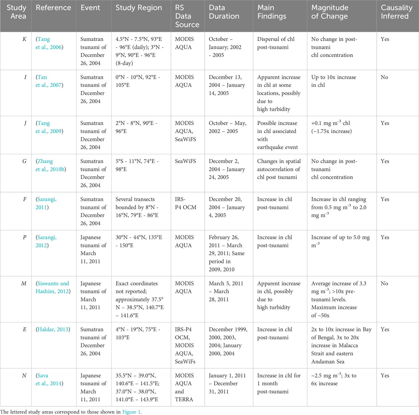
Table 1 Current literature in which remote sensing techniques were used to assess post-tsunami changes in chl, including the earthquake/tsunami event, study region, remote sensing data source, data duration, main findings of the study, and magnitudes of the observed changes.
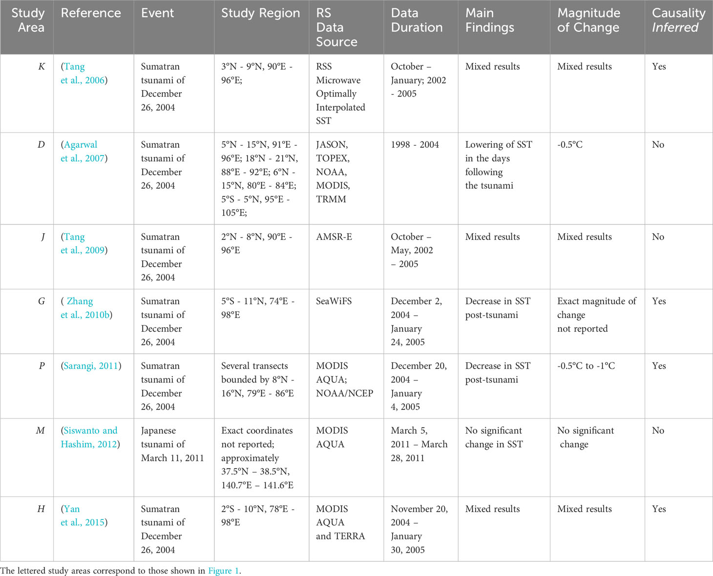
Table 2 Current literature in which remote sensing techniques were used to assess post-tsunami changes in SST, including the earthquake/tsunami event, study region, remote sensing data source, data duration, main findings of the study, and magnitudes of the observed changes.
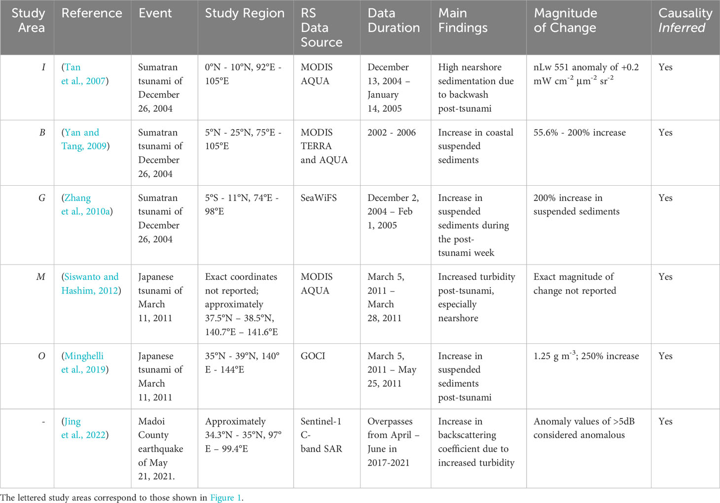
Table 3 Current literature in which remote sensing techniques were used to assess post-tsunami changes in turbidity, including the earthquake/tsunami event, study region, remote sensing data source, data duration, main findings of the study, and magnitudes of the observed changes.
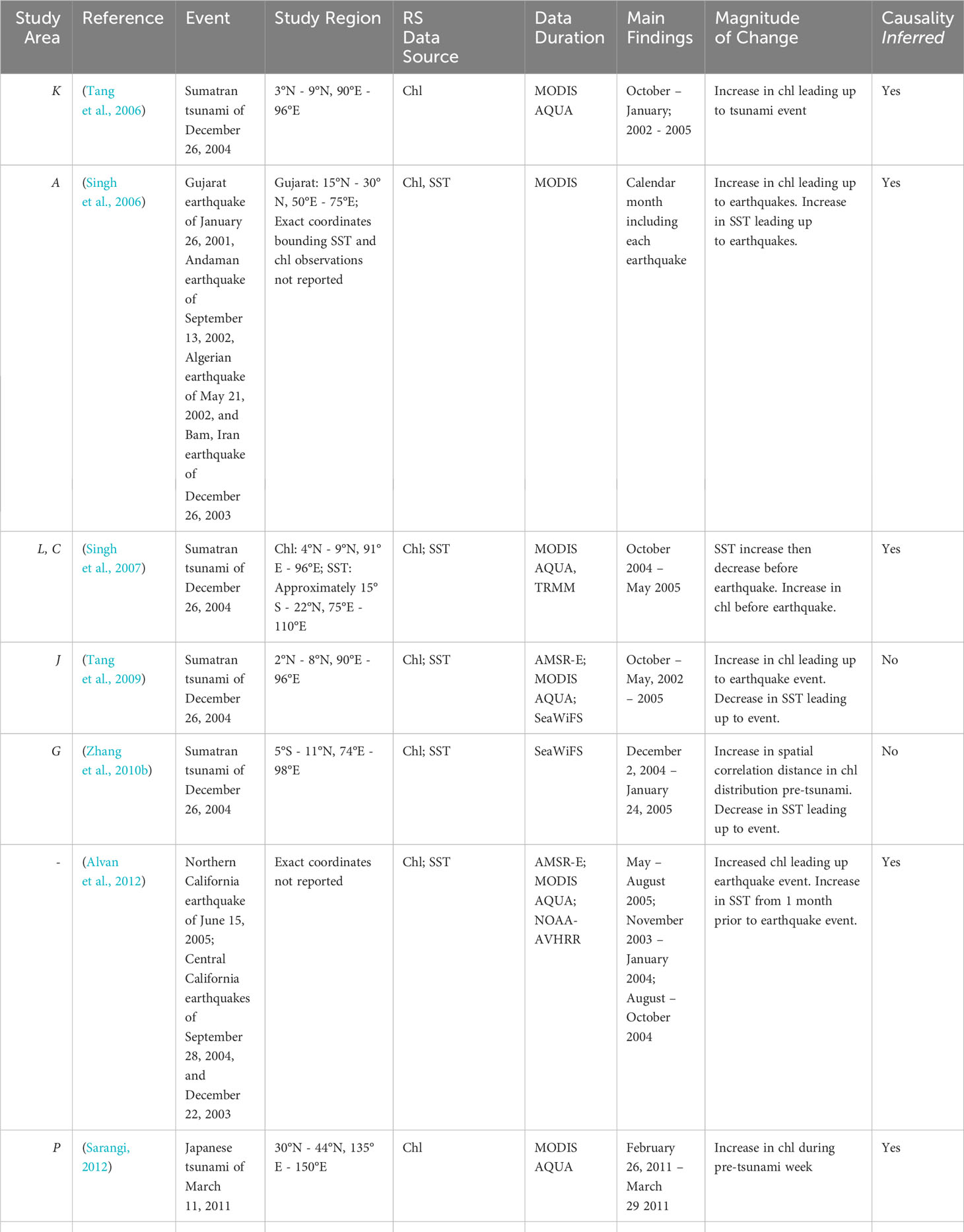
Table 4 Current literature in which remote sensing techniques were used to assess pre-seismic or pre-tsunami changes in oceanographic conditions, including the earthquake/tsunami event, study region, relevant oceanographic conditions reviewed in the study, remote sensing data source, data duration, and the main findings of the study.
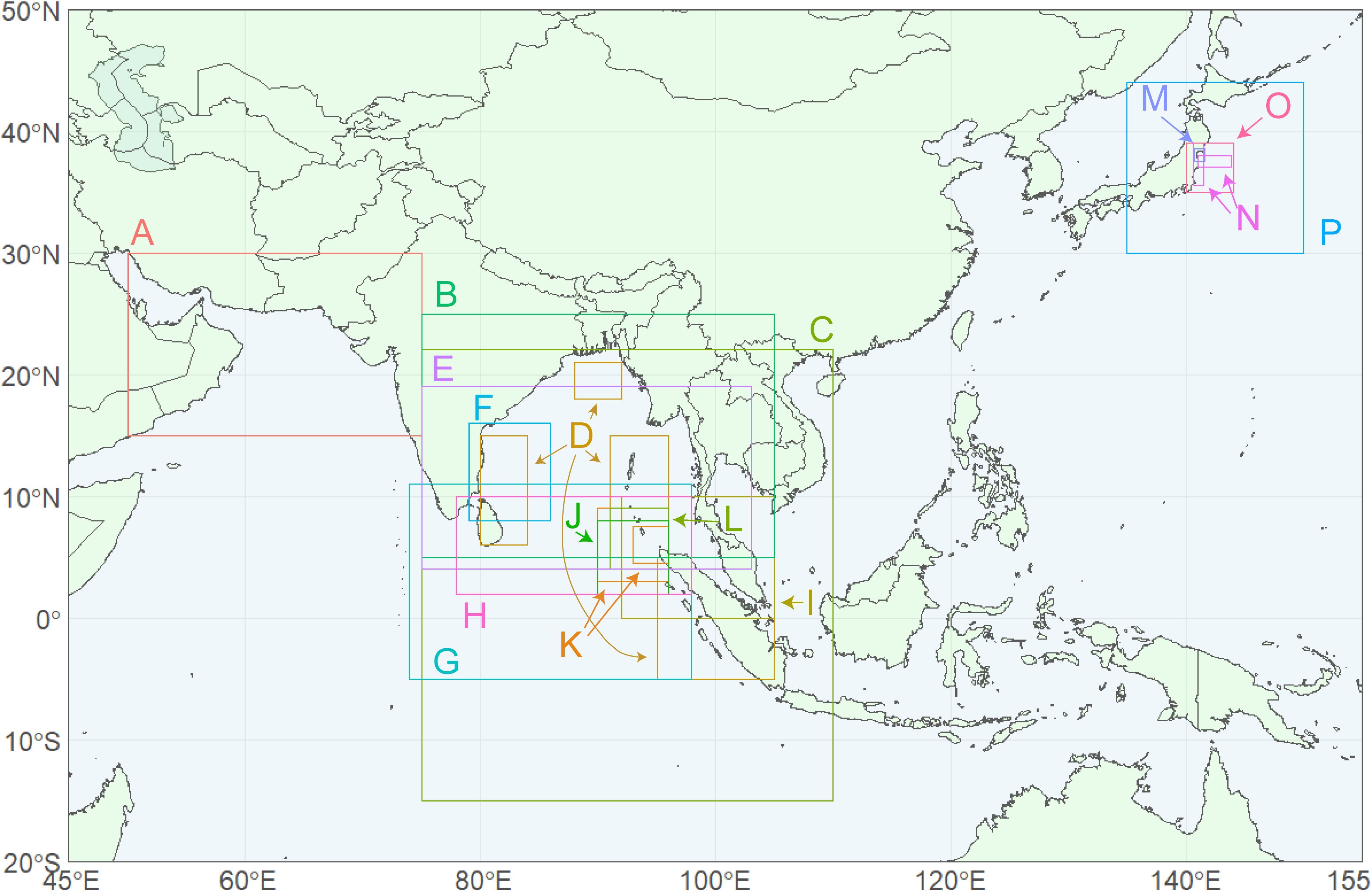
Figure 1 Summary figure showing study areas of the published papers and those in this review. Letters correspond to the study entries in Tables 1–4 below.
The existing literature reports that there is either no change or an increase in chl during the post-tsunami period, along with a change in the distribution of chl as indicated by remotely sensed data (Table 1). These studies were focused on either the Gujarat earthquake of January 26, 2001, the Sumatran tsunami of December 26, 2004, or the Japanese tsunami of March 11, 2011. The study areas included the epicenter of the tsunami-causing earthquakes and coastal waters near areas heavily impacted by the tsunamis. The spatial coverage of the time series in the studies varied from 1° squared to ~12,000 km2 to 15° squared (~2.8 million km2). Larger areas covering the Bay of Bengal and Andaman Sea were qualitatively inspected for changes in chl concentration and distribution in some studies of the 2004 Sumatran tsunami.
The time series duration used in these studies ranged from 16 days to 4 years. Time series used in the studies included daily, weekly (8-day), and monthly aggregated data for chl. A longer time series of weekly averages of chl was included as reference data in one study (Tang et al., 2009). In this study, weekly averaged SeaWiFS chl data from December 26, 1998 - March 30, 2004 were compared to weekly averages before and after the tsunami event.
Reported changes in chl ranged from no change to ~50x pre-tsunami levels, with some studies only reporting a qualitative change in concentration or distribution of chl based on visual inspection of the pre- and post-tsunami images. Tan et al. (2007) and Siswanto and Hashim (2012) noted that high turbidity caused by turbulent mixing in coastal areas may have contributed to higher remotely sensed chl than in situ chl values.
Qualitative changes in chl observed from visual inspection of satellite images were noted in several studies. Tan et al. (2007) noted decreased chl in Malacca Strait after the Sumatran tsunami of 2004, while increased chl was observed near Northwestern Sumatra (near epicenter) during the post-tsunami week. Sarangi (2011) observed increased chl in the eastern part of the Andaman Sea and Bay of Bengal along the coast of Myanmar during the post-tsunami period. The increased chl was observed to last for approximately ten days after the tsunami event. Using images before, during, and after the Japanese tsunami of 2011, Sarangi (2012) observed increased chl in coastal waters.
Research concerning tsunami-induced changes in SST has shown mixed results (Table 2). Observed changes in SST included decreased SST during the post-tsunami period, a combination of regional warming and cooling across the affected area, as well as no significant changes in SST during the post-tsunami period.
Of the papers that reported mixed results of both positive and negative SST changes during the post-tsunami period, Yan et al. (2015) reported an increase of up to 4°C in the area southwest of the epicenter of the 2004 Sumatran tsunami during the 4-day period after the event. The area southwest of Sri Lanka exhibited cooling of up to 2°C during the same period, after which increased SST was found, due to advection of surface waters from the epicenter. During this time, the southern Bay of Bengal encompassing the northern part of the study region exhibited no significant changes in SST.
Another study showing mixed results is Tang et al. (2006), where an increase in SST of 0.5°C to 1°C was found near the epicenter region, while significant cooling (up to 2°C) near the affected areas of Eastern India in the Bay of Bengal was found.
Tang et al. (2009) reported a decrease in SST near the epicenter region leading up to the tsunami, with a 1°C decrease in SST on the day of the tsunami event. Following this, an increase in SST of 1°C was reported in the week after the tsunami event. Low SST was observed in areas affected by the tsunami wave, such as the eastern coast of India in the Bay of Bengal. A lowering of SST of 1°C near the Andaman and Nicobar Islands in the eastern Bay of Bengal was reported on the day of the tsunami.
Three studies (Agarwal et al., 2007; Zhang et al., 2010a; Sarangi, 2011) reported an overall decrease of SST in the days following the tsunami. Agarwal et al. (2007) reported a decreased SST by an average of -0.5°C across the study regions during the 4-day period following the tsunami event. Zhang et al. (2010a) reported the lowest SST during the 8-day period after the tsunami event. Sarangi (2011) reported an overall decrease in SST of -0.5°C to -1.0°C.
After the 2011 Japanese tsunami event, the study by Siswanto and Hashim (2012) did not find any observable changes in SST as compared to pre-tsunami conditions. It should be noted that this study covered the smallest geographic study area (~1° × ~1°) among similar articles.
Several papers showed an increase in nearshore turbidity in tsunami-affected and earthquake-affected areas (Table 3). Offshore turbidity was noted not to increase substantially during the post-seismic period. Proposed mechanisms for the increased turbidity included backwash from tsunami-affected land areas (Tan et al., 2007) as well as resuspension of coastal sediments (Yan and Tang, 2009). One paper showed an increase in backscattering coefficient in terrestrial water bodies surrounding the epicenter of a seismic event, inferring that this increase was due to high turbidity in these water bodies caused by the earthquake (Jing et al., 2022).
Several studies noted changes in oceanographic conditions before the earthquake or tsunami events (Table 4). Both chl and SST were observed to change during the lead-up period to the seismic event. Chl was generally observed to increase before the seismic event, sometimes negatively correlated with SST in their spatial patterns (Tang et al., 2009; Zhang et al., 2010b). Although chl was observed to increase in all studies analyzing pre-seismic changes, changes in SST were mixed. SST was observed to increase before the seismic event reported in Singh et al. (2007); Alvan et al. (2012), and Zhang et al. (2022). However, SST was observed to decrease prior to the seismic event reported in Tang et al. (2009) and Zhang et al. (2010a).
One explanatory mechanism for the increased SST is a change in surface latent heat flux (SLHF) caused by a buildup of stress in the crust preceding the release of seismic energy (Singh et al., 2006; Singh et al., 2007; Alvan et al., 2012; Zhang et al., 2022). SLHF has been proposed by some to be a precursor signal for earthquakes (Dey and Singh, 2003). The increase in chl observed prior to the seismic event was attributed to increases in upwelling induced by changes in the thermal structure of the ocean indicated by changes in SLHF (Singh et al., 2006; Alvan et al., 2012; Zhang et al., 2022).
Zhang et al. (2010a) observed an increase in spatial correlation distance in chl distribution prior to the tsunami event, possibly a result of local transport via surface currents. The study stated that it was not clear whether this observation was a predictive precursor to the tsunami event.
Zhang et al. (2022) observed anomalies in SST and chl, among other atmospheric, land-based, and oceanic parameters. These anomalies were determined by a method modified from (Genzano et al., 2021) comparing the observed conditions compared to variation within a 10-year period. SST was observed to increase anomalously near the earthquake epicenter preceding the event and anomalous values, both positive and negative, were observed near plate boundaries preceding the event. An anomalous increase in chl was observed coinciding with the SST anomaly near the epicenter.
In addition to the remote sensing studies listed in Tables 1–4, there have also been in situ observations of post-tsunami changes in oceanographic conditions. These scarce observations yielded inconclusive results for chl and SST, but showed increased turbidity after the tsunami events (Table 5). However, it is difficult to know whether the increased turbidity was due to disturbance by the tsunami or other factors such as rainfall, while rainfall was discounted by Fiedler et al. (2014) as a possible factor leading to the post-tsunami changes in turbidity.
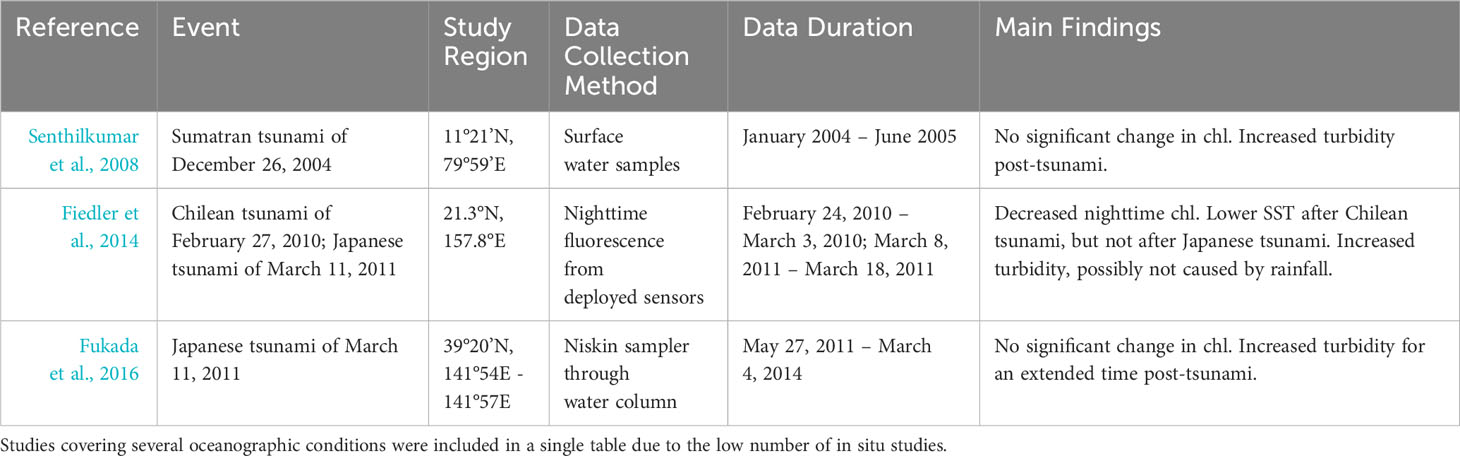
Table 5 Current literature in which in situ techniques were used to assess post-tsunami changes in chl, SST, and turbidity, including the tsunami event, study region, data collection method, data duration, and main findings of the study.
From these earlier studies, it is clear that certain ocean properties, either chl, turbidity, or SST, have been shown to change either before or after the earthquake/tsunami events. The question is whether such changes imply causality or simple coincidence. The former is of particular importance because if certain anomalies can be captured before earthquake/tsunami, such anomalies can be used as indicators to forecast earthquakes/tsunamis (Jiao et al., 2018; Picozza et al., 2021), which has significant implications on disaster management.
Recent reviews suggest that pre-seismic indicators are not consistent enough to forecast events regardless of magnitude (Picozza et al., 2021). Here, although some of the studies listed in Tables 1–4 attempted to elucidate precursory signals or other pre-seismic trends, it is unclear whether these signals are caused by the seismic events through some unexplained mechanisms or simply due to coincidence. Likewise, it is unclear whether the post-event anomalies are also a result of coincidence.
Indeed, determining causality in complex ecosystems is always challenging (Sugihara et al., 2012). For post-event response evaluations, the Granger causality paradigm (Granger, 1969) is difficult to achieve due to lack of complete time series of several independent variables to explain the dependent variable. Under such circumstances, a ‘control’ experiment may be conducted, where the ocean variables in the same region are examined in the absence of the Tsunami (or other) events. Unfortunately, although such a ‘control’ experiment or similar analysis was used to study changes in atmospheric or terrestrial parameters (Piscini et al., 2017; Jing et al., 2022), it was lacking in nearly all published papers listed in the above tables when evaluating post-tsuanmi ocean changes. Here, using two examples, we show the importance of such a ‘control’ experiment in determining (or disapproving) causality.
The first example is for the Sumatran tsunami of December 26, 2004. Figure 2 shows the changes in chl and SST before and after the tsunami event for a region of the Indian Ocean and Bay of Bengal bounded by 3°N - 9°N and 90°E - 96°E. This study area is the same as was used in Tang et al. (2006) and Tang et al. (2009). For the period of November 2004 – February 2005 encompassing the tsunami event, the results are similar to those reported in Tang et al., 2009, i.e., dramatic changes in Chl before the tsunami and minor changes in SST before and after the tsunami (red curves in Figure 2). These changes might infer causality at first glance. However, similar changes also occurred in other years in the absence of tsunami events (blue and green curves in Figure 2). Therefore, when these other years are used as the ‘control’ experiments, it is clear that the chl and SST changes around the tsunami event in December 2004 cannot be used to infer causality, but are likely due to a coincidence of natural variability.
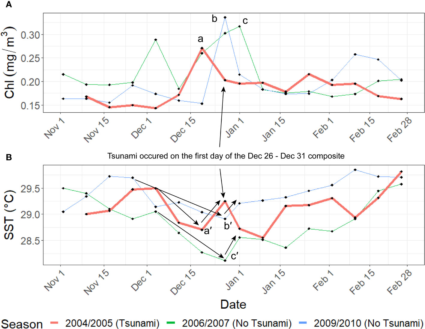
Figure 2 Time series of 8-day average values of (A) chl and (B) SST for November 1st through March 5th before and after the Sumatran tsunami of December 26th, 2004 (red curve, with the event annotated by a black arrow), in the area bounded by 3°N - 9°N and 90°E - 96°E. This bounding box was chosen to encompass the coastal, open ocean, and epicenter regions affected by the Sumatran tsunami of December 26, 2004, after Tang et al., 2006. Letters (a), (b), and (c) represent peaks in chl, which were preceded by a dip and then increase in SST, as annotated by (a′), (b′), and (c′).
One anomalous ‘spike’ in chl is present in the week before the tsunami during the tsunami season (Figure 2A). Inspection of the 8-day composite images suggests that this spike likely a result of spatial aliasing due to different cloud cover in the sequential composite images. As seen in Figure 3A, a large portion of the cloud-free data during the week of the chl spike (before tsunami) was in the near-shore areas around the Andaman and Nicobar Islands as well as in the northwestern Malacca Strait, which have relatively higher chl than in the nearby offshore waters to the southwest of Sumatra that were cloud free in the following week (Figure 3B). Such a difference in the distribution of cloud free data led to the dramatic changes in the average chl before and after the tsunami event (Figure 4 left side). However, if the comparison is restricted to the overlapping cloud free pixels in both periods (Figures 3C, D), the mean and median chl values are indeed similar between the two periods. Although there has been no field measurement or other source to validate the satellite observations, earlier evaluation results suggest that satellite-derived chl values in coastal waters typically have uncertainties of 25% - 75% (e.g., Cannizzaro et al., 2013), and their interpretations here should be valid especially when they are used as a relative index.
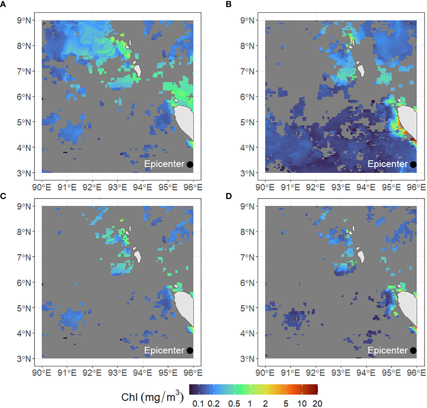
Figure 3 MODIS/Aqua 8-daily composite chl for (A, C) December 18-25, 2004, and (B, D) December 26-31, 2004, before and after the Sumatran Tsunami of December 26, 2004, respectively. (A, B) show the full extent of available cloud-free chl data while (C, D) show only those pixels with data available for both composites. Tsunami epicenter location is labeled by a black dot.
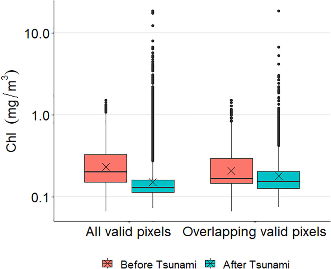
Figure 4 A quantile boxplot of chl values of the before-after composites from all available pixels (left, see Figures 3A, B) and from the overlapping pixels (right, see Figures 3C, D). The bottom, middle, and top bars of the boxes represent the 25%, 50%, and 75% percentile values, while the crosses represent the arithmetic averages.
Similar results were obtained for the Haldar et al. (2013) study when a ‘control’ experiment was conducted using non-tsunami years. Following Haldar et al. (2013), in the tsunami year, elevated chl was indeed found in the Bay of Bengal and Andaman Sea in the post-tsunami period (compare Figures 5A, C, E), especially the Eastern Andaman Sea and Malacca Strait regions (red ellipses in Figure 5) which comprise the continental shelf and slope regions. Based on this observation, one may speculate that the post-tsunami increases in chl could be due to the tsunami disturbance. However, similar elevated chl in the same regions was also found in the same periods but in non-tsunami years (Figures 5B, D, F). Therefore, from the chl changes alone, it is difficult to conclude whether the changes were due to the tsunami disturbance or due to natural variability.
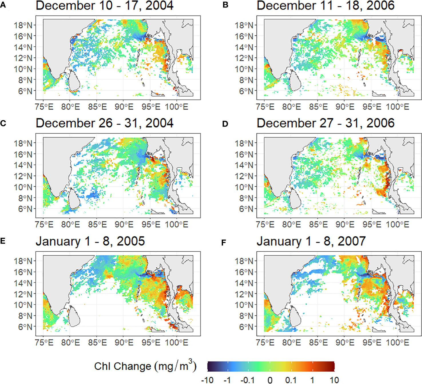
Figure 5 Composite chl anomaly images for the area bounded by 4°N - 19°N, 75°E - 103°E for the periods (A) December 10 -17, 2004, just before the Sumatran Tsunami of December 26, 2004; (B) December 11 – 18, 2006, the same period two years later; (C) December 26 – 31, 2004, just after the tsunami; (D) December 27 – 31, 2006, the same period two years later; (E) January 1 – 8, 2005, after the tsunami; and (F) January 1 – 8, 2007, the same period two years later. Red ellipse indicates the Eastern Andaman Sea region of interest.
The same findings were obtained for the case of the Japan tsunami of March 11, 2011 when a control experiment was used to diagnose the reason. Following Sava et al. (2014), chl showed substantial increases in both the epicenter region and affected coastal region, as shown in Figures 6A, B, respectively. Yet in other years without tsunami (2004, 2008, 2013), similar increases of chl in both regions were also found during the same periods. The timing and magnitude of the chl increases after the tsunami event were not unique as compared with those in the non-tsunami years, suggesting that it is difficult to relate the post-tsunami chl changes to tsunami disturbance. For example, in region A, chl values did not exceed 1 standard deviation from the historical mean (2003-2022) for any 8-day period following the tsunami (Figure 6A). In region B, while chl values did exceed 1 standard deviation on three occasions, several other years without a tsunami event also showed similar variation (Figure 6B). Expanding the analysis to the entire year further shows that the 2011 tsunami occurred right before the spring bloom (Figures 6C, D). Therefore, it is difficult to attribute the post-tsunami increase in chl to the 2011 tsuanmi.
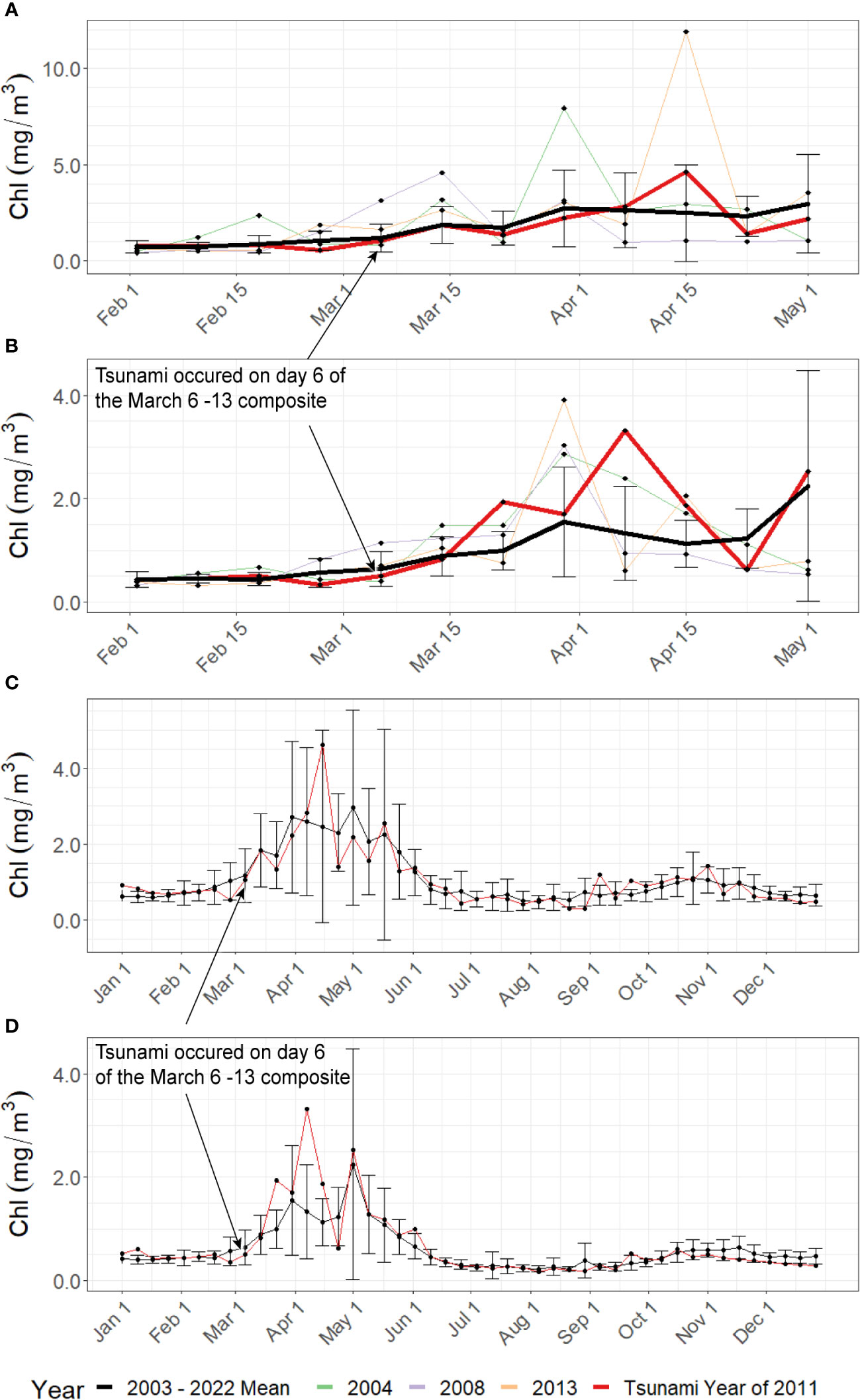
Figure 6 Time series of 8-day average chl in the area bounded by (A) 35°N - 39°N and 140°E - 141°E and (B) 37°N - 38°N and 141°E - 143°E. These bounding boxes were chosen to represent (A) the coastal regions of Japan affected by the Japanese tsunami of March 11, 2011, and (B) the epicenter and open ocean regions of Japan affected by the Japanese tsunami of March 11, 2011, after Sava et al. (2014). For comparison, the tsunami year and three other years as well as the 2003 – 2022 mean (vertical bars represent standard deviations) are shown in these graphs. In (C, D), the time series is extended to the entire tsunami year and the 2003 – 2022 climatology.
Similar findings were obtained from the RST-based spatial analysis (Ciancia et al., 2018) and the ALICE anomaly index (Sava et al., 2014) (Figure 7). While there are some areas of anomalously high chl in the regions, such anomalies also occur in non-tsunami years during this time of year with similar intensity and scale.
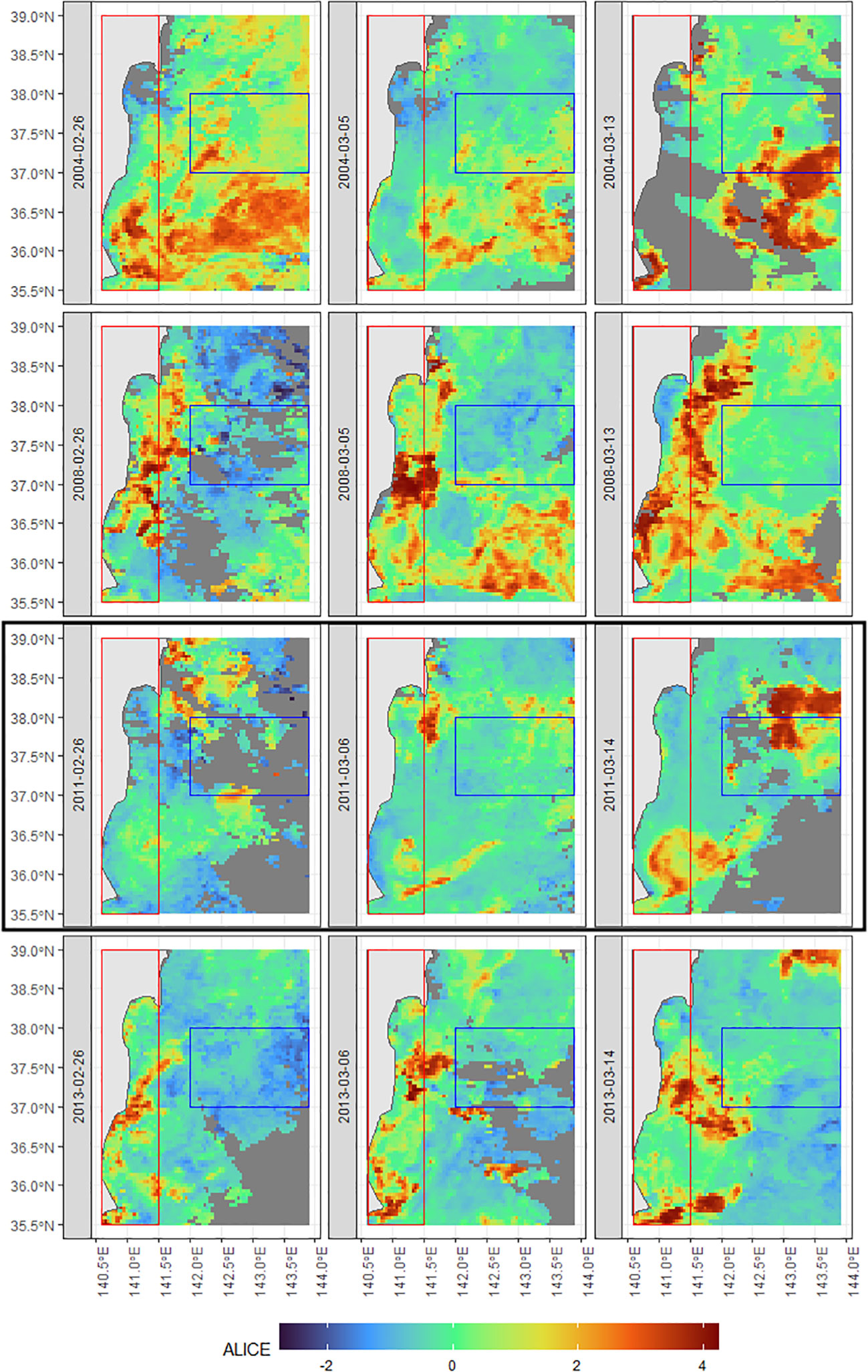
Figure 7 Chl anomaly off the coast of eastern Japan for the area 35.5°N - 39°N and 140.6°E – 143.9°E derived from the Robust Satellite Techniques (RST) after (Ciancia et al., 2018). Red and blue rectangles represent study areas R1 and R2, respectively, from (Sava et al., 2014). The tsunami year, 2011, is highlighted with a black rectangle. Color scale represents the Absolutely Local Index of Change of the Environment (ALICE) after (Tramutoli, 2007).
On exception in the published literature is Zhang et al. (2022), where a 10-year mean SST was used as the background to determine SST anomalies in the years with earthquake (2021) and without major seismicity (2011, 2014, 2017). Compared with these three other years, SST anomalies in selected regions right before and after the earthquake were apparent, thus being used to infer causality. However, we believe that in order to rule out other possible causes, one would need to examine all individual years instead of just 3 years. If no other year showed similar SST anomalies, then the argument for the causality would be stronger.
In addition to the counter arguments on the possible causality, this study also found that the published results cannot always be reproduced here, possibility due to different data reprocessing to account for instrument changes in calibration and stability. For example, Yan and Tang (2009) used a turbidity index to compare the concentration of suspended solids in the Bay of Bengal during the post-tsunami year and the same turbidity index in an average of other years, with the latter being used as a reference year. An increase in the turbidity index was found in each month during the post-tsunami year. However, this observation could not be reproduced here, as shown in Figure 8 where the post-tsunami year (green bars) did not stand out from the reference (red bars). Although the turbidity index in the post-tsunami year was greater than the reference for seven out of twelve months, most values were within one standard deviation of the reference, suggesting non-substantial changes.
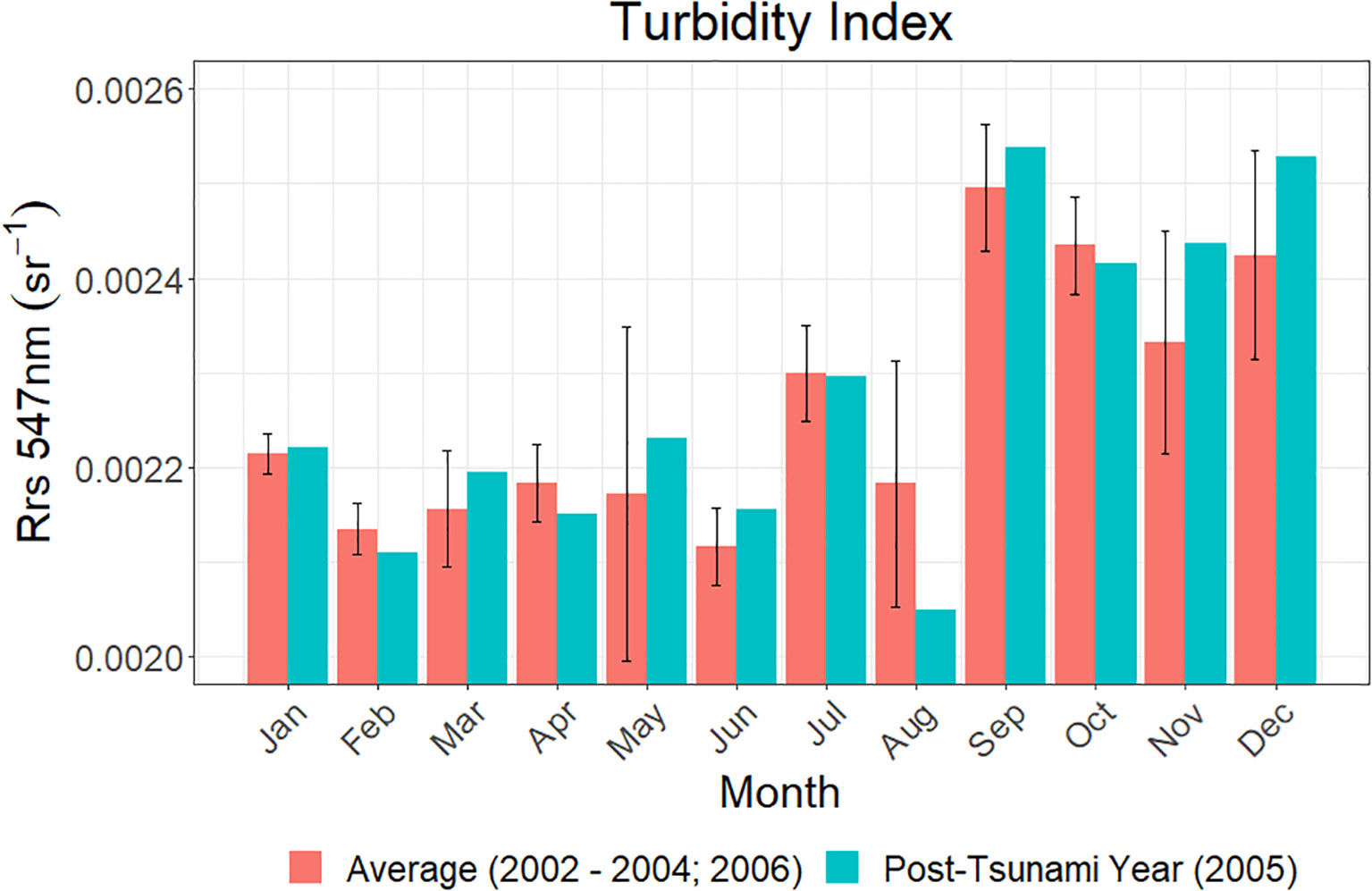
Figure 8 Monthly composite Rrs 547nm for the area 5°N - 25°N, 75°E - 105°E, used as a turbidity proxy comparing the year after the Sumatran tsunami (2005) to an average of the years 2002-2004 and 2006. Error bars represent the standard deviation of the monthly turbidity across the years used in the average. The Sumatran tsunami occurred on December 26, 2004, 5 days before the start of the post-tsunami year.
Note that all these new observations and arguments in this study are simply stating that, based on the before-after changes in the oceanographic properties (chl, SST, turbidity), one cannot jump to the conclusion that such changes are due to the seismic/tsunami events. This is certainly different from stating that these changes are not due to the seismic/tsunami events. This is because the former arguments only need to show that similar changes also occurred even without the seismic/tsunami events, but the latter arguments require further evidence to show that factors other than the seismic/tsunami events were indeed the reasons leading to the observed changes, and such evidence are typically very difficult to find. For example, two factors that can possibly lead to increased chl are photosynthetically available radiation (PAR) and winds, as the former is required by phytoplankton photosynthesis and latter may make deep-water nutrients available in surface waters to stimulate phytoplankton growth through either upwelling or deep mixing (Kahru et al., 2010). While PAR shows no apparent changes in the Sumatran tsunami year as compared with other years (Figure 9), the Sumatra study area experienced high winds in the Northern part of the study region in the weeks before the observed chl spike during the week of December 18 – 25, 2004 (Figure 10). Therefore, although such strong winds could not be used to disapprove the hypothesis that the increased chl was due to the tsunami disturbance, they did not approve the hypothesis either. Rather, they indicate that increased chl could be due to the strong winds.
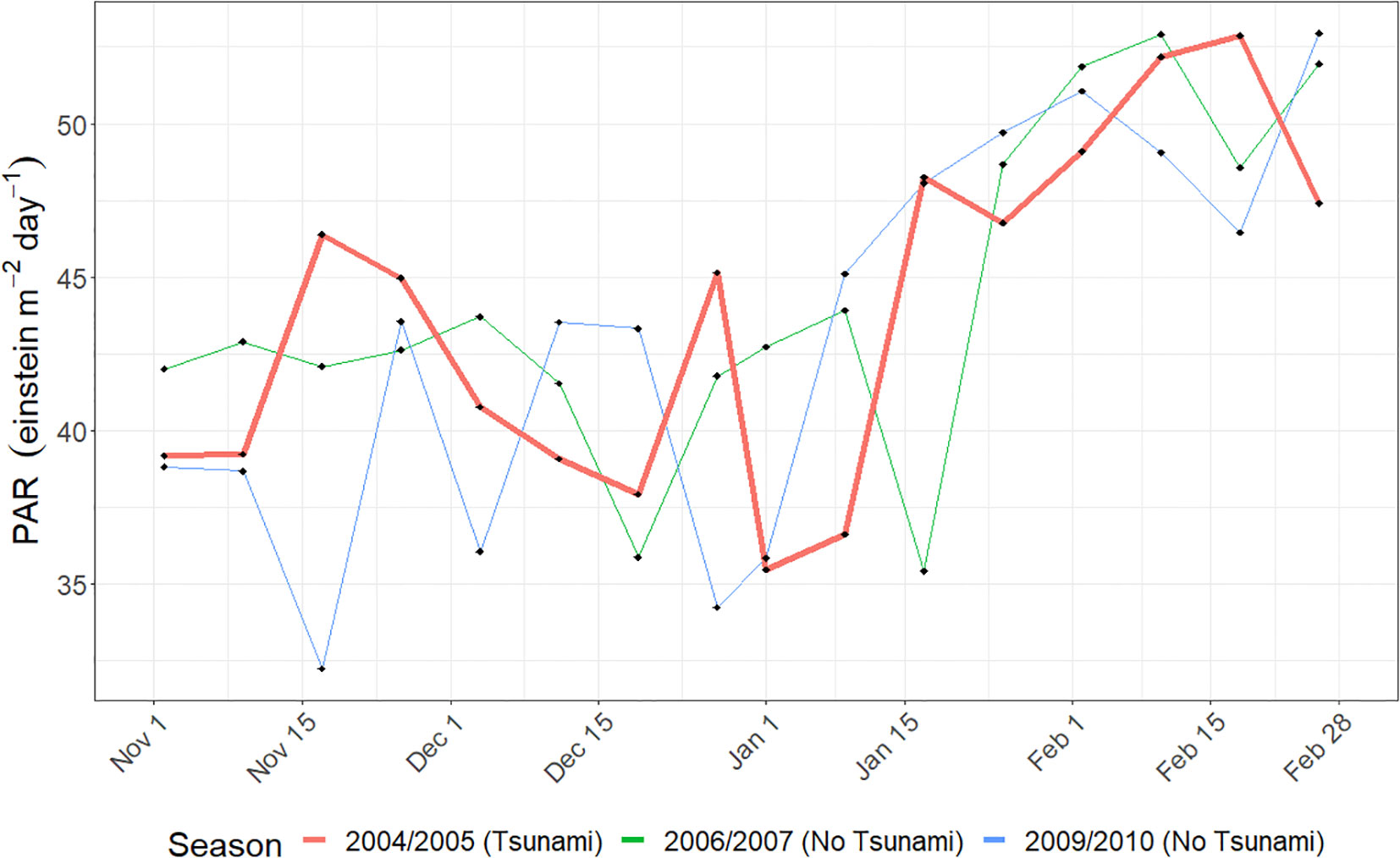
Figure 9 Time series of 8-day average PAR for November 1st through March 5th before and after the Sumatran tsunami of December 26th, 2004 (red curve), in the area bounded by 3°N - 9°N and 90°E - 96°E. Also plotted are the 8-day average PAR for other years.
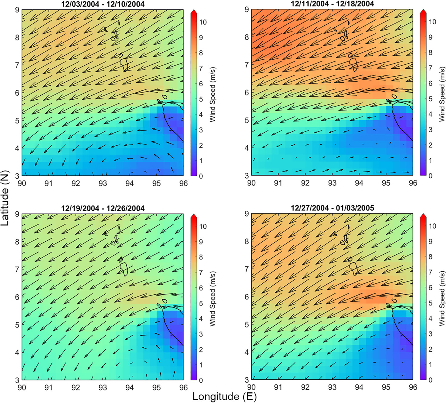
Figure 10 8-day wind speeds and directions in the area bounded by 3°N - 9°N and 90°E - 96°E for the periods before and after the Sumatran tsunami of December 26, 2004.
In short, although the existing evidence cannot rule out the possibility that the pre- or post-seismic/tsunami changes in ocean properties were due to the events, there is no evidence to suggest causality either. Furthermore, from the ‘control’ experiments conducted in this study, it is more likely that the observed changes are due to natural variability rather than the seismic/tsunami events. Therefore, the answer to the original question of “did tsunamis lead to changes in any ocean properties” is: maybe not.
Several studies in the published literature have proposed a causal relationship between seismic events and changes in ocean properties such as chlorophyll concentration, sea surface temperature, or turbidity. However, although most of these changes can be reproduced through the reanalysis here, similar changes are also found in other years without seismic events. It is therefore difficult to draw conclusions on the causality, but coincidence due to natural variability appears to be the possible reason behind the observed changes. Further work to differentiate potential seismic effects on ocean properties from natural variability is required to make claims about potential causal relationships. From this reanalysis, it is suggested that when causality were to be inferred from pre- or post-event changes, a ‘control’ experiment would be a minimal requirement to serve as a reference to contrast the observed changes. Although such a ‘control’ experiment is not able to show the exact reasons behind the observed changes in ocean properties, it does show that changes alone prior to or after the events are insufficient to infer causality.
SB: Writing – original draft, Writing – review & editing, Investigation. CH: Conceptualization, Supervision, Writing – review & editing, Funding acquisition.
The author(s) declare financial support was received for the research, authorship, and/or publication of this article. This work was supported by the U.S. NASA through its Ocean Biology and Biogeochemistry program and Ecological Forecast program (80NSSC20M0264, 80NSSC21K0422).
We thank NASA for providing satellite data for the reanalysis and thank Dr. Yingjun Zhang for analyzing surface winds. We also thank the reviewers for their valuable comments and suggestions.
The authors declare that the research was conducted in the absence of any commercial or financial relationships that could be construed as a potential conflict of interest.
All claims expressed in this article are solely those of the authors and do not necessarily represent those of their affiliated organizations, or those of the publisher, the editors and the reviewers. Any product that may be evaluated in this article, or claim that may be made by its manufacturer, is not guaranteed or endorsed by the publisher.
Agarwal V. K., Mathur A., Sharma R., Agarwal N., Parekh A. (2007). A study of air–sea interaction following the tsunami of 26 December 2004 in the eastern Indian Ocean. Int. J. Remote Sens. 28 (13–14), 3113–3119. doi: 10.1080/01431160601091837
Ahmad Z., Franz B. A., McClain C. R., Kwiatkowska E. J., Werdell J., Shettle E. P., et al. (2010). New aerosol models for the retrieval of aerosol optical thickness and normalized water-leaving radiances from the SeaWiFS and MODIS sensors over coastal regions and open oceans. Appl. Optics 49 (29), 5545–5560. doi: 10.1364/AO.49.005545
Alvan H. V., Azad F. H., Omar H. B. (2012). Chlorophyll concentration and surface temperature changes associated with earthquakes. Nat. Hazards 64 (1), 691–706. doi: 10.1007/s11069-012-0264-8
Alvan H. V., Mansor S., Omar H., Azad F. H. (2014). Precursory signals associated with the 2010 M8.8 Bio-Bio earthquake (Chile) and the 2010 M7.2 Baja California earthquake (Mexico). Arabian J. Geosci. 7 (11), 4889–4897. doi: 10.1007/s12517-013-1117-9
Cannizzaro J., Hu C., Carder K. L., Kelble C. R., Melo N., Johns E. M., et al. (2013). On the accuracy of SeaWiFS ocean color data products on the West Florida Shelf. J. Coast. Res. 29 (6), 1257–1272. doi: 10.2112/JCOASTRES-D-12-00223.1
Ciancia E., Coviello I., Di Polito C., Lacava T., Pergola N., Satriano V., et al. (2018). Investigating the chlorophyll-a variability in the Gulf of Taranto (North-western Ionian Sea) by a multi-temporal analysis of MODIS-Aqua Level 3/Level 2 data. Continental Shelf Res. 155, 34–44. doi: 10.1016/j.csr.2018.01.011
Dey S., Singh R. P. (2003). Surface latent heat flux as an earthquake precursor. Nat. Hazards Earth Syst. Sci. 3 (6), 749–755. doi: 10.5194/nhess-3-749-2003
Fiedler J. W., McManus M. A., Tomlinson M. S., De Carlo E. H., Pawlak G. R., Steward G. F., et al. (2014). Real-time observations of the February 2010 Chile and March 2011 Japan tsunamis: recorded in honolulu by the pacific islands ocean observing system. Oceanography 27 (2), 186–200.
Fukuda H., Katayama R., Yang Y., Takasu H., Nishibe Y., Tsuda A., et al. (2016). Nutrient status of Otsuchi Bay (northeastern Japan) following the 2011 off the Pacific coast of Tohoku Earthquake. J. Oceanogr. 72 (1), 39–52. doi: 10.1007/s10872-015-0296-2
Genzano N., Filizzola C., Hattori K., Pergola N., Tramutoli V. (2021). Statistical correlation analysis between thermal infrared anomalies observed from MTSATs and large earthquakes occurred in Japan, (2005–2015). J. Geophysical Research: Solid Earth 126 (2), e2020JB020108. doi: 10.1029/2020JB020108
Gordon H. R., Wang M. (1994). Retrieval of water-leaving radiance and aerosol optical thickness over the oceans with SeaWiFS: A preliminary algorithm. Appl. Optics 33 (3), 443–452. doi: 10.1364/AO.33.000443
Granger C. W. J. (1969). Investigating causal relations by econometric models and cross-spectral methods. Econometrica 37 (3), 424–438. doi: 10.2307/1912791
Haldar D., Raman M., Dwivedi R. M. (2013). Tsunami—A jolt for Phytoplankton variability in the seas around Andaman Islands: A case study using IRS P4-OCM data. Indian J. Mar. Sci. 42 (4), 437–447.
Hu C., Feng L., Lee Z., Franz B. A., Bailey S. W., Werdell P. J., et al. (2019). Improving satellite global chlorophyll a data products through algorithm refinement and data recovery. J. Geophysical Research: Oceans 124 (3), 1524–1543. doi: 10.1029/2019JC014941
Jiao Z.-H., Zhao J., Shan X. (2018). Pre-seismic anomalies from optical satellite observations: A review. Nat. Hazards Earth Syst. Sci. 18 (4), 1013–1036. doi: 10.5194/nhess-18-1013-2018
Jing F., Xu Y., Singh R. P. (2022). Changes in surface water bodies associated with madoi (China) Mw 7.3 earthquake of May 21, 2021 using sentinel-1 data. IEEE Trans. Geosci. Remote Sens. 60, 1–11. doi: 10.1109/TGRS.2022.3170890
Kahru M., Gille S. T., Murtugudde R., Strutton P. G., Manzano-Sarabia M., Wang H., et al. (2010). Global correlations between winds and ocean chlorophyll. J. Geophysical Research: Oceans 115 (C12). doi: 10.1029/2010JC006500
Levin B. W., Nosov M. (2016). Physics of Tsunamis (Switzerland: Springer International Publishing). doi: 10.1007/978-3-319-24037-4
Li R.-R., Kaufman Y. J., Gao B.-C., Davis C. O. (2003). Remote sensing of suspended sediments and shallow coastal waters. IEEE Trans. Geosci. Remote Sens. 41 (3), 559–566. doi: 10.1109/TGRS.2003.810227
Minghelli A., Lei M., Charmasson S., Rey V., Chami M. (2019). Monitoring suspended particle matter using GOCI satellite data after the Tohoku (Japan) tsunami in 2011. IEEE J. Selected Topics Appl. Earth Observations Remote Sens. 12 (2), 567–576. doi: 10.1109/JSTARS.2019.2894063
National Geophysical Data Center. (2021). Global Historical Tsunami Database (United States: NOAA National Centers for Environmental Information). doi: 10.7289/V5PN93H7
O’Reilly J. E., Werdell P. J. (2019). Chlorophyll algorithms for ocean color sensors—OC4, OC5 & OC6. Remote Sens. Environ. 229, 32–47. doi: 10.1016/j.rse.2019.04.021
Picozza P., Conti L., Sotgiu A. (2021). Looking for earthquake precursors from space: A critical review. Front. Earth Sci. 9. doi: 10.3389/feart.2021.676775
Piscini A., De Santis A., Marchetti D., Cianchini G. (2017). A Multi-parametric Climatological Approach to Study the 2016 Amatrice–Norcia (Central Italy) Earthquake Preparatory Phase. Pure Appl. Geophys. 174 (10), 3673–3688. doi: 10.1007/s00024-017-1597-8
Sarangi R. K. (2011). Remote sensing of chlorophyll and sea surface temperature in Indian water with impact of 2004 Sumatra tsunami. Mar. Geodesy 34 (2), 152–166. doi: 10.1080/01490419.2011.571561
Sarangi R. K. (2012). Impact assessment of the Japanese tsunami on ocean-surface chlorophyll concentration using MODIS-Aqua data. J. Appl. Remote Sens. 6 (1), 63539. doi: 10.1117/1.JRS.6.063539
Sava E., Edwards B., Cervone G. (2014). Chlorophyll increases off the coasts of Japan after the 2011 tsunami using NASA/MODIS data. Nat. Hazards Earth Syst. Sci. 14 (8), 1999–2008. doi: 10.5194/nhess-14-1999-2014
Senthilkumar B., Purvaja R., Ramesh R. (2008). Seasonal and tidal dynamics of nutrients and chlorophyll a in a tropical mangrove estuary, southeast coast of India. Indian J. Mar. Sci. 37 (2), 9.
Singh R. P., Cervone G., Kafatos M., Prasad A. K., Sahoo A. K., Sun D., et al. (2007). Multi-sensor studies of the Sumatra earthquake and tsunami of 26 December 2004. Int. J. Remote Sens. 28 (13–14), 2885–2896. doi: 10.1080/01431160701237405
Singh R. P., Dey S., Bhoi S., Sun D., Cervone G., Kafatos M. (2006). Anomalous increase of chlorophyll concentrations associated with earthquakes. Adv. Space Res. 37 (4), 671–680. doi: 10.1016/j.asr.2005.07.053
Siswanto E., Hashim M. (2012). A data fusion study on the impacts of the 2011 Japan tsunami on the marine environment of Sendai Bay. Int. J. Image Data Fusion 3 (2), 191–198. doi: 10.1080/19479832.2012.674064
Stumpf R. P., Arnone R. A., Gould R. W., Martinolich P. M., Ransibrahmanakul V. (2003). A partially coupled ocean-atmosphere model for retrieval of water-leaving radiance from SeaWiFS in coastal waters. NASA Tech. Memo 206892, 51–59.
Sugihara G., May R., Ye H., Hsieh C., Deyle E., Fogarty M., et al. (2012). Detecting causality in complex ecosystems. Science 338 (6106), 496–500. doi: 10.1126/science.1227079
Tan C. K., Ishizaka J., Manda A., Siswanto E., Tripathy S. C. (2007). Assessing post-tsunami effects on ocean colour at eastern Indian Ocean using MODIS Aqua satellite. Int. J. Remote Sens. 28 (13–14), 3055–3069. doi: 10.1080/01431160601091787
Tang D., Satyanarayana B., Zhao H., Singh R. P. (2006). A preliminary analysis of the influence of Sumatran tsunami on Indian ocean Chl-a and SST. Adv. Geosci. 5, 15–20. doi: 10.1142/9789812707215_0003
Tang D., Zhao H., Satyanarayana B., Zheng G., Singh R. P., Lv J., et al. (2009). Variations of chlorophyll-a in the northeastern Indian Ocean after the 2004 South Asian tsunami. Int. J. Remote Sens. 30 (17), 4553–4565. doi: 10.1080/01431160802603778
Tramutoli V. (2007). “Robust satellite techniques (RST) for natural and environmental hazards monitoring and mitigation: theory and applications,” in 2007 International Workshop on the Analysis of Multi-temporal Remote Sensing Images (Leuven, Belgium), 1–6. doi: 10.1109/MULTITEMP.2007.4293057
Walton C. C., Pichel W. G., Sapper J. F., May D. A. (1998). The development and operational application of nonlinear algorithms for the measurement of sea surface temperatures with the NOAA polar-orbiting environmental satellites. J. Geophysical Research: Oceans 103 (C12), 27999–28012. doi: 10.1029/98JC02370
Yan Z., Sui Y., Sheng J., Tang D., Lin I.-I. (2015). Changes in local oceanographic and atmospheric conditions shortly after the 2004 Indian Ocean tsunami. Ocean Dyn. 65 (6), 905–918. doi: 10.1007/s10236-015-0838-6
Yan Z., Tang D. (2009). Changes in suspended sediments associated with 2004 Indian Ocean tsunami. Adv. Space Res. 43 (1), 89–95. doi: 10.1016/j.asr.2008.03.002
Zhang L., Jiang M., Jing F. (2022). Sea temperature variation associated with the 2021 Haiti Mw 7.2 earthquake and possible mechanism. Geomatics Natural Hazards Risk 13 (1), 2840–2863. doi: 10.1080/19475705.2022.2137439
Zhang X., Tang D., Li Z., Dai X. (2010a). Spatio-temporal dynamics of suspended sediment concentration during the 2004 Sumatra tsunami. Indian J. Mar. Sci. 39 (3), 10.
Keywords: tsunami, earthquake, chlorophyll, turbidity, sea surface temperature, remote sensing
Citation: Bunson S and Hu C (2023) Did tsunamis lead to changes in ocean properties? a revisit. Front. Mar. Sci. 10:1275445. doi: 10.3389/fmars.2023.1275445
Received: 10 August 2023; Accepted: 21 November 2023;
Published: 11 December 2023.
Edited by:
Kiichiro Kawamura, Yamaguchi University, JapanReviewed by:
Angelo De Santis, National Institute of Geophysics and Volcanology (INGV), ItalyCopyright © 2023 Bunson and Hu. This is an open-access article distributed under the terms of the Creative Commons Attribution License (CC BY). The use, distribution or reproduction in other forums is permitted, provided the original author(s) and the copyright owner(s) are credited and that the original publication in this journal is cited, in accordance with accepted academic practice. No use, distribution or reproduction is permitted which does not comply with these terms.
*Correspondence: Chuanmin Hu, aHVjQHVzZi5lZHU=
Disclaimer: All claims expressed in this article are solely those of the authors and do not necessarily represent those of their affiliated organizations, or those of the publisher, the editors and the reviewers. Any product that may be evaluated in this article or claim that may be made by its manufacturer is not guaranteed or endorsed by the publisher.
Research integrity at Frontiers
Learn more about the work of our research integrity team to safeguard the quality of each article we publish.