Characterization of extreme wave fields during Mediterranean tropical-like cyclones

The Mediterranean Sea is a primary source of food, ecosystem services and economic activities and one of the most active cyclogenetic regions in the world, where the influence of orographic and morphological features of the relatively small basin plays an important role. Together with the explosive cyclogenesis, tropical-like cyclones (also called Mediterranean Hurricanes or Medicanes) are among the strongest types of storms that can be found in the Mediterranean basin, occurring predominantly in the Ionian, Balearic and Tyrrhenian sub-basins. Similarly to tropical cyclones (Hurricanes or Typhoons), these cyclonic structures are characterized by strong rotating and translating wind fields, which often lead to a combination of remotely generated swell waves and locally generated wind waves, often referred to as crossing sea states. Despite the well-known potential of Medicanes to cause significant damage near islands and coastal zones, which is predicted to intensify as a result of climate change, to date the characterization of maximum individual waves generated during these events is still lacking. In this study, we carry out the first analysis of the large-scale geographical distribution of wave maxima within the wave fields generated during three recent Medicane events using the WAVEWATCH III® spectral wave model forced by ERA5 reanalysis winds, also investigating the influence of crossing sea states on the maximum wave amplitudes with novel statistical formulations developed for such conditions. Our results show that, as in the case of tropical cyclones, several regions of the cyclone field are characterized by crossing sea states, whose role in the formation of the maximum individual waves occurring near the eye of the storm was found to be confined. Furthermore, extreme wave predictions accounting for the local crossing conditions yield differences up to 5% compared to standard statistical distributions.

1 Introduction

Mediterranean tropical-like cyclones (MTLC; Cavicchia et al., 2014) are mesoscale disturbances that manifest tropical-like characteristics, especially around the eye, with a morphology similar to tropical cyclones (TC; see Emanuel, 2005), without visible frontogenesis in the mature stage. In general, due to both the physical processes that intensify the cyclone and the region in which it develops, their ground structure varies considerably. Indeed, although tropical-like storms have also been observed in the Atlantic Ocean (Franklin et al., 2006) and Black Sea (Efimov et al., 2008), they occur predominantly in the Mediterranean Sea (and are therefore also known as Medicanes), particularly in the Ionian, the Balearic, and the Tyrrhenian sub-basins (see Patlakas et al., 2021), where the topography and coastal morphology play a key role in determining the near-surface wind fields and consequently the genesis and evolution of the wave fields, more frequently in late summer and autumn. Medicanes are rare compared to other cyclones that occur in the Mediterranean Sea, since they originate in a baroclinic environment, albeit still requiring several atmospheric conditions to produce a barotropic environment. The frequency of occurrence varies according to the type of MTLC considered: if only very strict criteria are adopted, i.e. only storms with fully tropical features (such as cloud structure, degree of symmetry, dimensions, and lifespan on satellite images), 0.5 events occur per year on average, while if hybrid structures are also included around 1.5 Medicanes per year occur (Cavicchia et al., 2014).

The great potential of Medicanes to cause widespread hydrogeological instability and significant infrastructural and economic damage due to storm surges and extremely large waves, especially near islands and coastal zones, is of primary concern for marine and coastal safety, design and operations both in the present and in the future climate, with some recent studies suggesting that climate change could lead to an intensification of the strongest events (Cavicchia et al., 2014; Tous et al., 2016; González-Alemán et al., 2019).

While the characterization of the wave fields in cyclone conditions has been an active topic of research for decades and has been studied extensively (Moon et al., 2003; Liu et al., 2017; Young, 2017), the formation of individual, extreme waves is a process whose understanding is still underway and may be explained by several competing mechanisms (Mori, 2012; Jiang et al., 2019; McAllister et al., 2019; Benetazzo et al., 2021a).

Indeed, for the case of tropical cyclones, it was suggested that extreme waves caused by nonlinear four-wave interactions (modulational instability) in narrow-banded, long-crested wave conditions might occur southeast of the storm centre in the Northern Hemisphere, while in the south and west areas of the cyclone, the rapidly varying, rotating wind and wave fields lead to different combinations of remotely generated swell waves and locally generated wind waves, also called crossing seas, depending on the position with respect to the cyclone eye and track (see Wright et al., 2001; Black et al., 2007; Hu and Chen, 2011; Holthuijsen et al., 2012; Mori, 2012; Liu et al., 2017). Although crossing seas can potentially possess enhanced growth rate of modulational instability, in realistic ocean conditions the effect of nonlinear four-wave focusing is largely reduced by the spectral broadening (Onorato et al., 2009; Waseda et al., 2009; Fedele et al., 2016) and the formation of extreme waves is then driven mostly by second-order bound wave interactions (Adcock et al., 2011; Brennan et al., 2018; McAllister et al., 2018). However, the role of interacting wind sea and swell waves in the generation of high waves during cyclone conditions is still an open issue, with potentially dangerous implications both at sea and in coastal areas.

As regards Medicane events, existing studies on the wave fields generated during such extreme conditions have only focused on the significant wave height (Varlas et al., 2020; Patlakas et al., 2021; Ferrarin et al., 2023), while the characterization of the highest individual waves is still lacking.

In this context, we investigate the large-scale distribution of spatio-temporal maximum individual waves under strong winds associated with three recent MTLC events by combining a state-of-the-art spectral wave model and the short-term/range space-time extreme wave statistics.

The goal of this analysis is, on the one hand, to characterize the extreme wave field during a Medicane for the first time, comparing it with the field produced under the more typical case of a tropical cyclone. On the other hand, we aim at investigating the influence of crossing seas generated during the selected events on the magnitude of extremes, using a parametrization recently proposed by Davison et al. (2022).

The paper is structured as follows. In Section 2 we describe the numerical model setup used for the hindcast carried out in this work and we outline the second-order statistical model that was adopted for the space-time extreme wave statistical analysis for both unimodal and crossing sea conditions. In the same section we also provide details on the generation of the three tropical-like cyclones considered in this study. In Section 3, after characterizing the modelled cyclone wind and wave fields during peak conditions and assessing the model performance against in-situ and remote-sensing observations, we outline the spatial patterns of maximum individual waves, comparing two different types of spatio-temporal analysis. Then, we describe the local crossing conditions obtained from a spectral partitioning procedure and we analyse their influence on the distribution of extremes around the cyclone eye. Finally, conclusions are summarized in Section 4, where the strengths and limits of the methodology employed are also highlighted.

2 Materials and methods

2.1 Wave model setup and space-time extreme wave prediction

In the present study, for the analysis of the spatio-temporal fields of extreme waves we have employed a numerical model hindcast, produced by running the wave model WAVEWATCH III^® version 6.07 (hereinafter WW3; The WAVEWATCH III Development Group WW3DG, 2019) over a high-resolution structured curvilinear grid with a horizontal spacing of 0.05° (about 5 km) and on a spectral domain with 32 frequencies (f₁ = 0.05 Hz with 1.1 geometric progression) and 36 evenly (10°) spaced directions from 5° to 355° N. The wave model was forced with the 10-meter wind speed horizontal components provided by the ERA5 hourly atmospheric reanalysis with a 0.25° resolution horizontal structured grid (Hersbach et al., 2020), which was recently used for the assessment of extreme wave climatology in the Mediterranean Sea (Barbariol et al., 2021). Although poor performances of ERA5 extreme winds have been observed during warm-core tropical cyclones (Campos et al., 2022) as well as near the coast (Barbariol et al., 2022; Benetazzo et al., 2022), the choice to use a reanalysis as the atmospheric forcing stems from the fact that, no optimal setup exists for the simulation of extreme events such as MTLCs (Pytharoulis et al., 2018), so ERA5 has the advantage of assimilating available observations during the cyclone life-span. Indeed, even a multi-physics ensemble does not necessarily lead to an improvement in the overall reproduction of the cyclone (Ferrarin et al., 2023), and only a modelling approach including fully coupled numerical models with high spatial and vertical resolutions and dedicated parameterization and optimization for extreme tropical weather grants a more accurate overall description of the air–sea interaction processes (Ricchi et al., 2019). Aware of the inherent limitations in accurately describing the cyclone dynamics, our interest in this work is rather in investigating the geographical pattern of wave extremes during selected Medicane events and relating it to the more common case of tropical cyclones. Nonetheless, to quantify the error committed using this model setup, WW3 wave performance are assessed in this study against satellite-borne and buoy data (see Section 3.2).

In WW3, wind input and dissipation were parametrized using the ST4 source-term of Ardhuin et al. (2010), relying on the default values with some adjustment of the coefficients (${\beta }_{max}$= 1.55 and $z_{0,max}$ = 0.002) in agreement with the results of TEST405 (The WAVEWATCH III Development Group WW3DG, 2019), which is suited for short fetch conditions. Wave propagation has been computed using a third-order accurate scheme and the nonlinear energy transfer among wave components is approximated using the discrete interaction approximation (DIA; Hasselmann et al., 1985). For the definition of the bottom topography and the coastlines we have used the ETOPO1 relief model (doi: 10.7289/V5C8276M).

The hourly wave model outputs considered in this study are the directional wave energy spectrum $S\left(\omega ,\theta \right)$, the significant wave height H_s and the expected value (usually denoted with an overbar) of the space-time maximum crest height $C_{max}$.

Under the assumption of a stationary and homogeneous wave field $\eta \left(x,y,t\right)$, the expected value of $C_{max}$ over a fixed space-time region Γ ∈ IR³ of duration D and sea surface 2D region of orthogonal sides X and Y can be computed using the space-time extreme WW3 model implementation, distributed since version 5.16 (see Barbariol et al., 2017; Benetazzo et al., 2021b and references therein for more details on the spatio-temporal theoretical framework). Since the realistic sea states considered in this work are mostly characterized by broad-banded spectra in both wavenumber and direction (and are therefore not significantly affected by nonlinear four-wave interactions), we have considered as output the second-order nonlinear approximation for maximum crest heights derived by Benetazzo et al. (2015) and Fedele et al. (2017):

$\begin{array}{ll}\frac{{\overline{C}}_{max}}{H_s}=h_N+2\mu h_N^2+\gamma \left(1+4\mu h_N\right){(16h_N-\frac{32N_3{h}_N+4N_2}{16N_3{h}_N^2+4N_2{h}_N+N_1})}^{-1}& (1)\end{array}$

where $h_N$ is the dimensionless most probable extreme value (viz., the mode), $\mu$ represents the bulk wave steepness parameter (see Section 2.2), while N₃, N₂ and N₁ are proportional to the average number of waves within Γ of volume V=XYD, on the 2D boundary surfaces S of Γ and along the 1D perimeter B of Γ, respectively (see Baxevani and Rychlik, 2006; Fedele, 2012):

$\begin{array}{ll}{N}_3=2\pi \frac{XYD}{L_x{L}_y{T}_z}\sqrt{1-{\alpha }_{xt}^2-{\alpha }_{xy}^2-{\alpha }_{yt}^2+2{\alpha }_{xt}{\alpha }_{xy}{\alpha }_{yt}}& (2)\end{array}$

$\begin{array}{ll}{N}_2=\sqrt{2\pi }\left(\frac{XD}{L_x{T}_z}\sqrt{1-{\alpha }_{xt}^2}+\frac{YD}{L_y{T}_z}\sqrt{1-{\alpha }_{yt}^2}+\frac{XY}{L_x{L}_y}\sqrt{1-{\alpha }_{xy}^2}\right)& (3)\end{array}$

$\begin{array}{ll}{N}_1=\frac{X}{L_x}+\frac{Y}{L_y}+\frac{D}{T_z}& (4)\end{array}$

where L_x is the mean wavelength (evaluated along the mean wave direction), L_y is the mean crest length orthogonal to L_x, T_z is the zero-crossing average period, and α_xt, α_xy and α_yt are irregularity parameters (all ranging between -1 and 1) computed from the moments of the directional spectrum, which give a measure of the degree of organization of the 3D wave motion (Baxevani and Rychlik, 2006). In the limit of a directionally narrow-banded sea, the additional term $\sqrt{1-{\alpha }_{xt}^2-{\alpha }_{xy}^2-{\alpha }_{yt}^2+2{\alpha }_{xt}{\alpha }_{xy}{\alpha }_{yt}}$ becomes equal to zero, while for the other extreme case of a confused sea it becomes equal to 1.

As already mentioned above, sea states occurring during a cyclone are often characterized by the presence of multiple (crossing) wave systems. To isolate these distinct wave components (mostly wind sea and swells) at each model grid point we use topographic partitions and partition wave-age cut-off (WW3 default scheme, see also Hanson and Phillips, 2001), so additional model outputs are the main statistical parameters for each wave system, i.e. the significant wave height H_s, the peak wave period T_p, the peak wave length L_p and the peak wave direction ${\theta }_p$ of the wind sea (partition 1) and of a set of swell components ordered by decreasing wave height (partition 2,3,4,…), These parameters will be used for the computation of wave extremes in crossing conditions, as described in the following Section.

2.2 A second-order nonlinear model for maximum wave crest heights in crossing seas

In the literature, several statistical models have been developed and validated for extreme wave crest heights. In particular, while models were initially suited to time series of the sea surface displacement $\eta$ from a reference level at a single fixed point in time (t), they were recently extended to a spatial region (x,y) of given area larger than zero to account for the 3D geometry of very large waves, and are therefore also known as space-time extreme models (see Section 2.1). Regardless of the wavefield dimensionality considered, statistical models for extreme wave crest heights differ mainly for their varying degree of nonlinearity, whose effect is to distort the shape of the wave profile compared to the linear case, resulting in higher and sharper crests and shallower and flatter troughs. For instance, to second-order, the density mass is spread toward the higher crests in proportion to the magnitude of the wave steepness, as shown in Equation 1, following the Tayfun quadratic equation (Tayfun, 1980):

$$\xi =z+2\mu z^2$$

where $\xi =C_2/H_s$ is the dimensionless second-order crest height and $z=C_1/H_s$ is the linear counterpart.

Following Fedele and Tayfun (2009), the bulk wave steepness $\mu$ is usually evaluated as a statistically stable estimate from the moments of the directional spectrum, considering narrowband conditions with all component waves travelling in the same direction (i.e. long-crested or weakly spread), and is written in the following form:

$\begin{array}{ll}\mu =k_m\left(1-\upsilon +{\upsilon }^2\right)\sigma & (5)\end{array}$

where the two quantities:

$$k_m=\frac{1}{g}{\left(\frac{m_{001}}{m_{000 }}\right)}^2$$

$$\upsilon =\sqrt{\frac{m_{000 }{m}_{002}}{m_{001}^2}-1}$$

represent an integral measure of the mean wavenumber (Fedele and Tayfun, 2009) and the spectral bandwidth (Longuet-Higgins, 1975), respectively. The zeroth, first and second-order moments $m_{000 }$, $m_{001}$ and $m_{002 }$ of the directional spectrum are computed as:

$$m_{ijl}=\iint k_x^i{k}_y^j{\omega }^{l}S\left(\omega ,\theta \right)d\omega d\theta$$

where (k_x, k_y) is the wavenumber vector associated with the frequency f (through the linear dispersion relation for sea waves), $\omega =2\pi f$ is the angular frequency and $\theta$ is the wave direction (throughout this study, we adopt the direction of flow). We note that, since directional spreading effects are not included in the wave steepness parametrization used at present, Equation 5 represents an upper bound in directional seas, where the crest heights are generally reduced by directional spreading effects compared to unidirectional conditions (Toffoli et al., 2006; Onorato et al., 2009; McAllister and van den Bremer, 2019). However, following a similar approach to McAllister and van den Bremer (2019), the influence of directionality could in principle also be included.

Notwithstanding, since the bulk wave steepness computed from the directional wave spectrum was derived for the case of long-crested, narrowband conditions, when both swell and wind sea are present at the same time and location the formulation of Equation 5 fails to represent the wave geometry in a physically consistent way, due to the fact that it cannot be directly associated with the characteristics of either the constituent wave systems (Portilla et al., 2015; Trulsen et al., 2015; Luxmoore et al., 2019; Støle-Hentschel et al., 2020; Kanehira et al., 2021) and that the long-crested, narrowband approximation rarely holds. Indeed, when a crossing sea state is present, the formation of extreme waves depends on additional factors, such as the relative crossing angle between the two coexisting wave systems or their frequency ratio, which affect the strength of the wave-wave nonlinear interactions (Adcock et al., 2011; McAllister et al., 2018). To account for such effects, Davison et al. (2022) recently introduced a parametrization of the crossing wave steepness, which is based on the spectral characteristics of the two wave systems (mean wavenumber and spectral bandwidth, while the effect of directional spreading is not explicitly included) and on their local crossing conditions, which are characterized using three main parameters defined by Rodriguez et al. (2002) and Guedes Soares and Carvalho (2003): the Sea-Swell Energy Ratio (SSER), which represents the ratio of the variance associated with each wave system, the Intermodal Distance (ID), representing the frequency difference between the swell and wind waves spectral peaks, and the relative crossing angle ($\text{Δ}\theta$). These crossing sea parameters are expressed as follows:

$\begin{array}{ll} SSER=\frac{m_{000,w}}{m_{000,s}}& (6)\end{array}$

$\begin{array}{ll} ID=\frac{f_{P,w}-f_{P,s}}{f_{P,w}+f_{P,s}}& (7)\end{array}$

$\begin{array}{ll}\Delta \theta =\left|{\theta }_{P,w}-{\theta }_{P,s}\right|& (8)\end{array}$

where the subscript p represents the peak value of the considered variable (frequency or direction), while the subscripts w and s stand for wind sea and swell, respectively.

In particular, wave fields with SSER values smaller than 1.0 represent swell-dominated sea states (which are usually characterized by lower steepness values and therefore display almost Gaussian statistics, see Petrova and Guedes Soares, 2009), while wave conditions with SSER larger than 1.0 represent wind sea-dominated sea states. Similarly, when ID approaches 0, the sea state is characterized by a small frequency separation between swell and wind sea, while values of ID above 0.10 correspond to a sea state with clearly separated swell and wind sea peak frequencies. For the relative crossing angle, we refer to a following condition when the swell travels within 45° of the wind sea and to an opposing condition when the crossing angle lies in the range 135-180° (Donelan et al., 1997), while for angles between 45°-135° we use the wording orthogonal condition rather than cross swell, to avoid possible confusion with the more general definition of crossing seas.

The wave steepness parametrization for two quasi-monochromatic crossing wave groups (hereinafter referred to as ${\mu }_{crossing}$), stemming from Davison et al. (2022), can therefore be written as:

$\begin{array}{ll}{\mu }_{crossing}=(\frac{k_S}{{(1+\tau )}^2}+\frac{k_W}{{\left(1+\frac{1}{\tau }\right)}^2}+\frac{2\left(B^{+}+B^{-}\right)}{\left(1+\tau \right)\left(1+\frac{1}{\tau }\right)})\sigma & (9)\end{array}$

where $\tau =\sqrt[4]{SSER}$, while $k_W$ and $k_S$ are characteristic wavenumbers of wind sea and swell, respectively. For consistency with the unimodal distributions used at present, they are taken as $k_W=k_{m,W}\left(1-{\upsilon }_W+{\upsilon }_W^2\right)$ and $k_S=k_{m,S}\left(1-{\upsilon }_S+{\upsilon }_S^2\right)$ in order to include the effect of a finite spectral bandwidth for each unidirectional wave system (${\upsilon }_W$ and ${\upsilon }_S$), so that in the limit of $\tau \to 0$ (swell) and $\tau \to \infty$ (wind sea) Equation 9 coincides with Equation 5.

The coefficients $B^{+}$ and $B^{-}$, on the other hand, represent the second-order frequency-sum (+) and frequency-difference (-) interaction kernels for the nonlinear bound harmonics of two crossing wave groups, first introduced by Longuet-Higgins (1963) for deep water and then extended by Sharma and Dean (1979); Dalzell (1999) and Forristall (2000) to finite-depth directional seas. In the most general case, apart from the water depth d, both kernels are functions of the frequency ratio between the two interacting wave groups (viz. ID) and the relative crossing angle ($\text{Δ}\theta$), giving a total contribution whose general behaviour is illustrated in Figure 1.

Figure 1

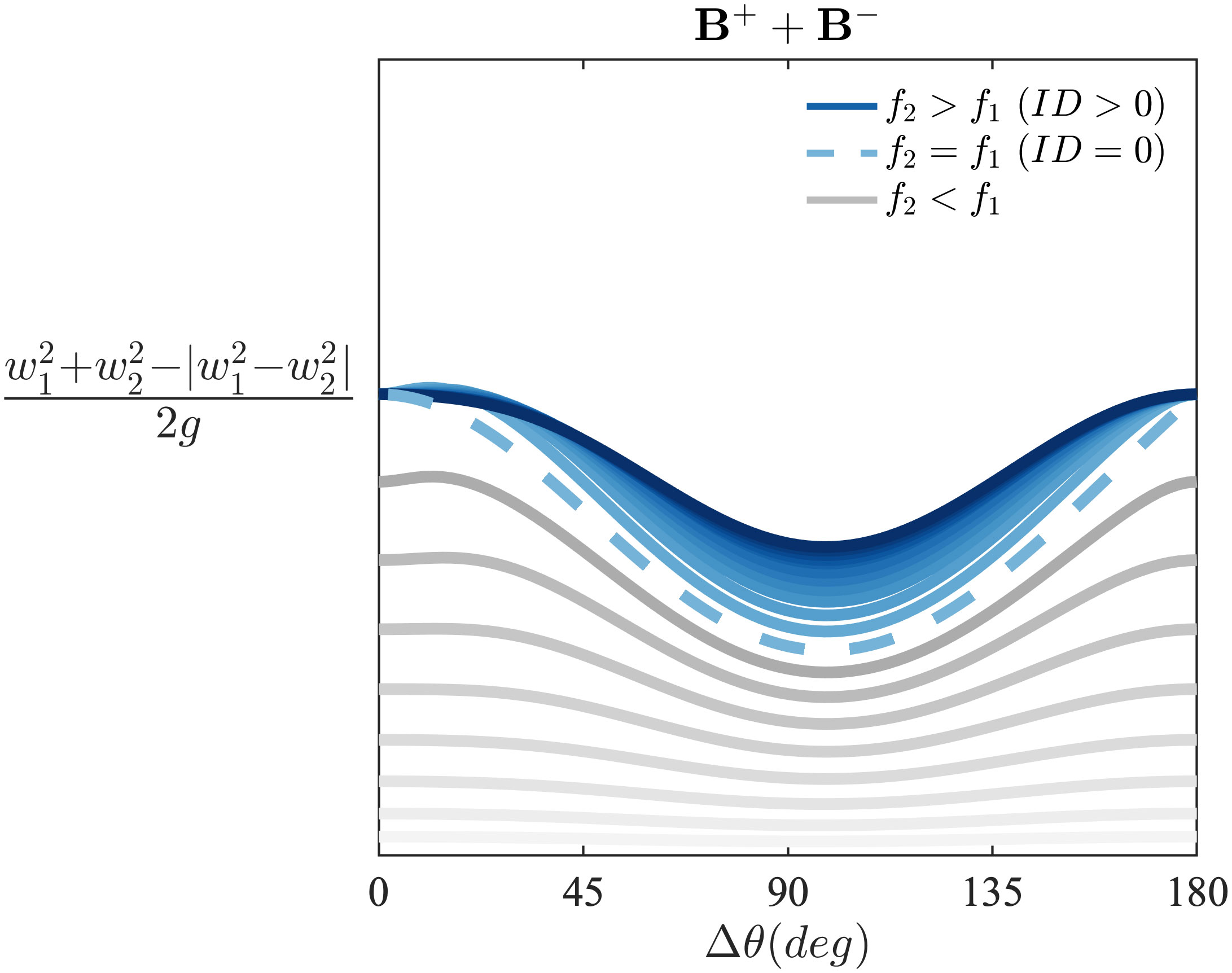
Figure 1 Total second-order interaction kernel for two crossing waves (where system 1 and 2 are taken to be the swell and wind sea, respectively) as a function of their peak frequency ratio $f_2/f_1$ and crossing angle $\text{Δ}\theta$. The line color becomes progressively darker as the frequency ratio increases from small values ($f_2<f_1$, grey solid lines) to large values ($f_2>f_1$, blue solid lines), while the simple case of $f_2=f_1$ is highlighted with a dashed line.

As the crossing angle increases, the sum of the subharmonic and superharmonic bound wave interactions reaches a minimum around 90° (a condition for which nonlinear interactions were found to be weak by e.g. Trulsen et al., 2015; see also McAllister and van den Bremer, 2019), whose magnitude is larger for crossing waves that result from wind sea and swell systems of different frequencies (ID > 0) compared to two wave systems of identical frequencies (ID = 0). Conversely, for both small (two wave systems travelling in the same direction) and large (two wave trains travelling in opposite directions) crossing angles the total wave-wave interaction term attains peak values (Tayfun, 2006; Christou et al., 2009).

We note that, compared to the formulation proposed by Davison et al. (2022), in the present work we consider the case of two in-phase wave systems (${\varphi }_W={\varphi }_S=0$), so the simple value of the superharmonic interaction kernel is taken instead of its absolute value, thus leading to a smaller increase of the wave steepness values for large crossing angles, where $B^{+}$ is usually negative.

For the characterization of maximum individual waves in crossing seas, Equation 9 can thus be used in the space-time extreme formulation of Equation 1, which will then be referred to as ${\overline{C}}_{max,crossing}$ to distinguish it from the maximum expected crest height ${\overline{C}}_{max}$ computed with the bulk wave steepness $\mu$ of Equation 5.

2.3 Medicanes Zorbas, Ianos and Apollo

Among the most recent MTLC events that affected the Ionian Sea, the most notable were Zorbas in late September 2018, Ianos in mid-September 2020 and Apollo in late October 2021, which were thus selected for the present study.

Medicane Zorbas developed in the Gulf of Sirte on 27 September 2018, moved first toward the Ionian Sea and then towards Greece, making landfall onto the Greek coasts on 29 September (red solid line in Figure 2). This MTLC was classified as one of the strongest ever observed (with intensity comparable to a Category 1 hurricane) and reached a mature tropical stage a few hours before landfall. Zorbas affected mainly the regions in southwestern Greece, especially Crete, the Peloponnese, Evia, and the region around Athens, producing considerable damage through severe winds, torrential rainfall, major flooding and even tornadoes. Along the coast, the wind speed reached 20 m/s, while offshore winds exceeded 40 m/s, as observed by ASCAT satellites (Figa-Saldaña et al., 2002).

Figure 2

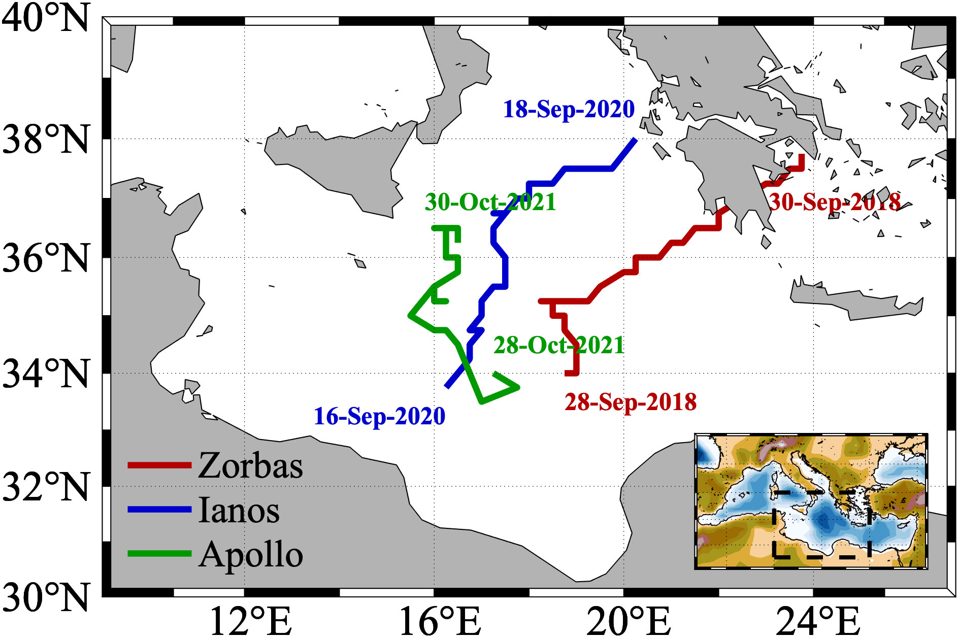
Figure 2 Trajectories of Zorbas (red), Ianos (blue) and Apollo (green) during their most intense phases in the Ionian Sea derived from the ERA5 reanalysis. The beginning and end dates of the plotted trajectories are also indicated. In the inset plot, the Mediterranean region and the Ionian Sea (dashed box) are shown for reference.

Similarly, cyclone Ianos started as an extratropical cyclone on 15 September 2020 while moving across the Ionian Sea, made a first landfall as a fully-grown MTLC around Greece on 18 September (blue solid line in Figure 2) and after turning south with the characteristics of an extratropical cyclone between 19-20 September, it reached the North African coasts, with a second landfall on 21 September on the Libyan coast. The areas most affected by Ianos were the Ionian Islands (Zakynthos, Kefalonia and Ithaca), Crete as well as some areas of the southern Italian regions of Sicily and Calabria. Ianos caused massive flooding due to storm surges, strong winds up to 45 m/s and gusts close to 50 m/s, as well as heavy rainfalls, which in some areas reached 500 mm/48h (Lagouvardos et al., 2022).

Lastly, Apollo developed near the Libyan coast on 25 October 2021 and moved north, towards the coasts of eastern Sicily and central-western Ionian Sea, becoming more intense due to the high temperatures of the Mediterranean Sea, and assumed the typical features of a Medicane on 28 October (green solid line in Figure 2). The main regions affected by the passage of the Apollo were the Italian areas between Catania, Messina and Siracusa (Sicily), with huge coastal flooding, wind speeds up to 33 m/s along the Sicilian coast (accelerated by the effect of local topography) and intense precipitations, with a peak of 448 mm/48 h recorded by the Sicilian Meteorological service near Catania (Borzì et al., 2022).

The cyclone tracks of the aforementioned events during their most intense phases, identified by pinpointing the minimum from the mean sea level pressure fields of the ERA5 reanalysis, are presented in Figure 2.

3 Results

3.1 Wind and wave fields during Zorbas, Ianos and Apollo

The MTLCs investigated in this study all exhibit a common origin, arising from extratropical cyclogenesis, baroclinic wave cut-off and warm seclusion. Interestingly, however, their ground structure varies considerably, as shown in Figure 3, where we illustrate reanalysis fields of 10-m wind speed U₁₀ and corresponding wave model fields of significant wave height H_s at the time instants at which the peak conditions were reached by the three cyclones during their mature stage.

Figure 3

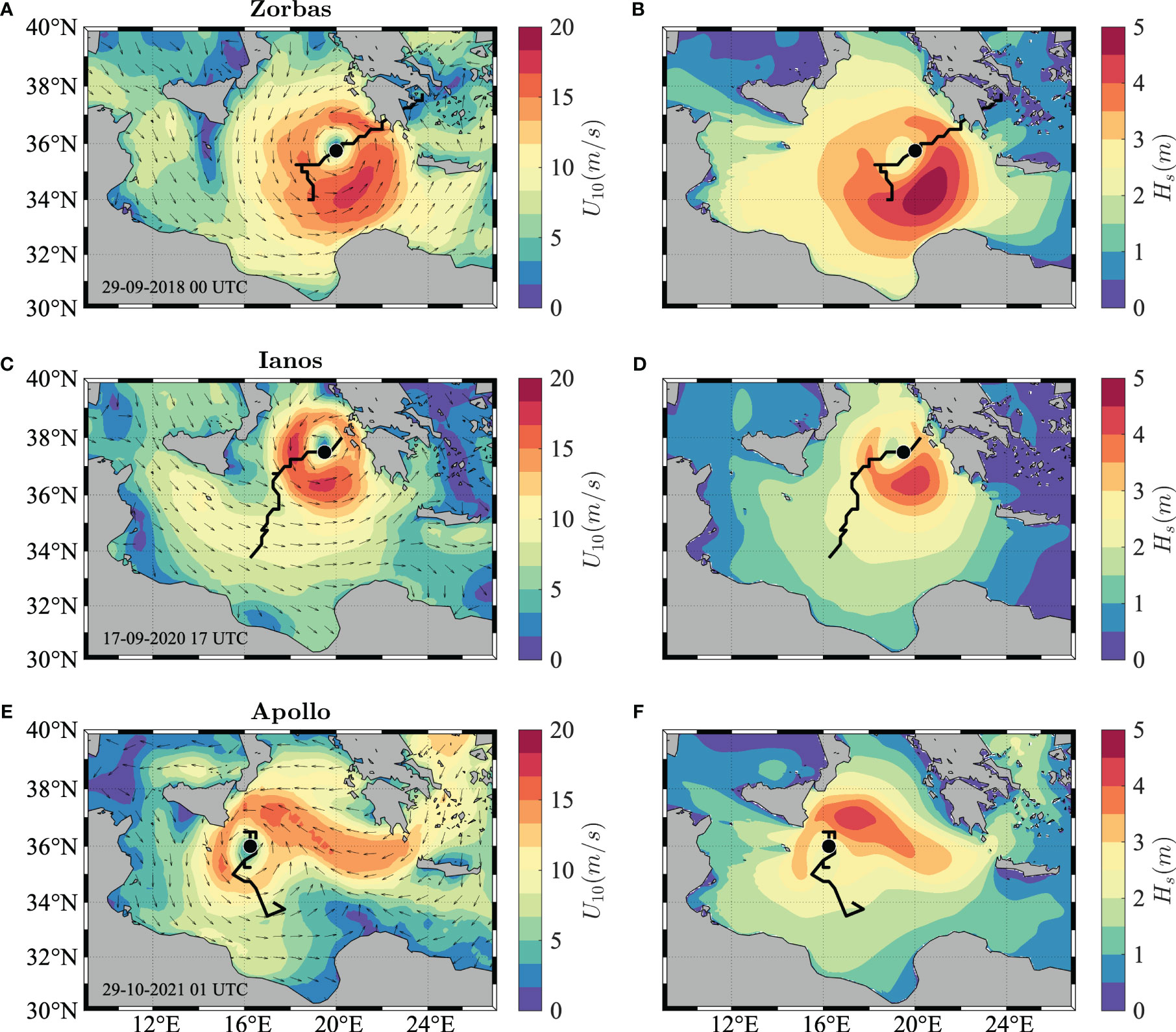
Figure 3 Wind and wave conditions in the Mediterranean Sea during the mature stages of Zorbas (A, B), Ianos (C, D) and Apollo (E, F). (A, C, E) ERA5 near-surface (10-m height) wind speed U₁₀ (colored shading) and direction (arrows, decimated for graphical purposes). The trajectories of the three MTLC derived from the ERA5 reanalysis are also shown with a black line, while the black marker indicates the position of the pressure minimum at the time instant at which the wind field is displayed. (B, D, F) Corresponding model significant wave height H_s (colored shading).

Indeed, while Zorbas and Ionas display a closed structure and extremely high winds around the cyclone eye, typical for instance of tropical cyclones, Apollo is characterized by significantly lower wind speeds and frontal (convergent) structures connected to the pressure minimum.

In particular, during Zorbas the highest wind speeds (U₁₀ around 20 m/s on 29 September 2018 at 00 UTC) occurred in the right quadrants of the cyclone, with respect to its southwest to northeast trajectory, where the highest waves were thus generated (H_s up to 6 m), since they move forward with the storm and therefore remain in the more intense wind regions for an extended period of time (the so-called “extended fetch”; see e.g., Young, 2003). A similar spatial pattern is also observed during Ianos, where the highest wind speeds (U₁₀ around 20 m/s on 17 September 2020 at 17 UTC) occurred in the bottom-right sector of the translating storm, although the wind field was somewhat more limited, compared to Zorbas, due to the presence of the Italian coast to the west and the Greek coast to the east. As a result, the corresponding wave field shows a slightly constrained pattern and a smaller spatial extent, with the highest significant wave heights in the right quadrant of the cyclone (H_s around 4 m). Conversely, during Apollo the cyclone evolution was more complex, with a larger extent of the wind field albeit with lower wind speed values (U₁₀ around 16 m/s on 29 October 2021 at 01 UTC) due to the strong winds blowing from the Peloponnese and a partial constraint by the southern Italian peninsula. The corresponding wave field shows the highest significant wave heights (H_s exceeding 4 m) where the largest fetch is present, i.e. in the top-right quadrant of the cyclone.

3.2 Assessment of model waves

The wave fields of the three MTLCs analyzed herein have been assessed using satellite altimeter observations of H_s retrieved from the Integrated Marine Observing System database (IMOS, https://catalogue-imos.aodn.org.au; Ribal and Young, 2019; Young and Ribal, 2019; only data flagged as “good data” were used). To this end, wave hindcast data have been bi-linearly interpolated in space and linearly interpolated in time on the satellite data points and the hindcast model performance have been evaluated using the model-minus-observation bias (BIAS) and the Mean Absolute Error (MAE). The comparison between significant wave height Ku band altimeter measurements from Jason-2 and Jason-3 satellites and the wave model hindcast during the three MTLCs Zorbas, Ianos and Apollo is shown in Figure 4.

Figure 4

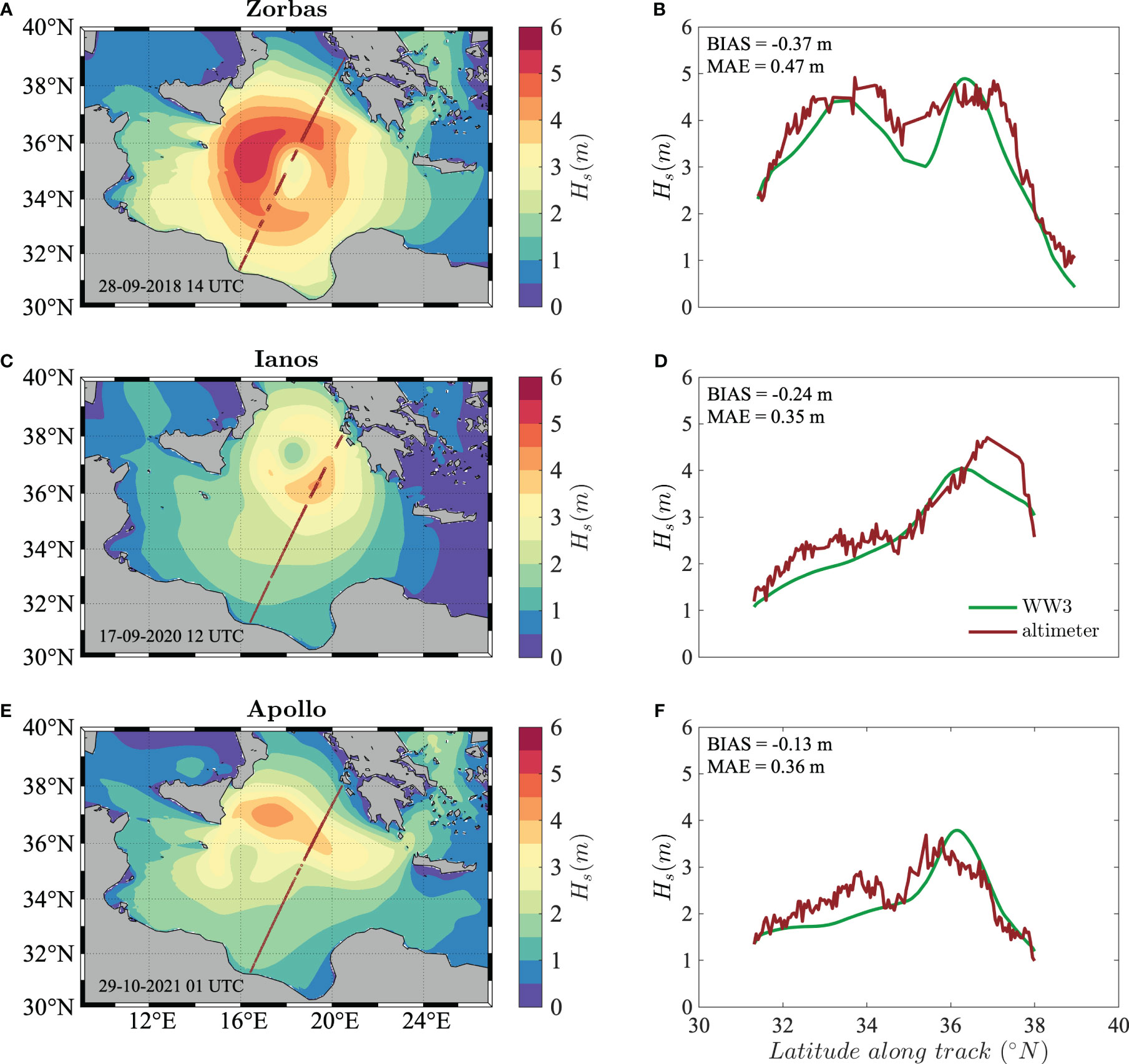
Figure 4 Comparison of significant wave height H_s between WW3 model and Ku band altimeter measurements during Zorbas (A, B), Ianos (C, D) and Apollo (E, F). (A, C, E) Model wave fields and the altimeter track (brown line). (B, D, F) Significant wave height measured by Jason-2 and Jason-3 altimeters (brown line) and from the numerical model along the satellite tracks (green line).

Overall, we see that during Zorbas on 28 September 2018 at 14:00 UTC the significant wave height from model data reached values around 5 m, with a slight underestimation compared to the altimeter data (BIAS = -0.37 m, MAE = 0.47 m), possibly due to the coarseness of the wind forcing, which lacks the necessary resolution to capture the fine scale structures of the cyclone near the eye, thereby propagating uncertainties and errors to the wave model results (Abdolali et al., 2021). Similar performances (BIAS = -0.24 m, MAE = 0.35 m) were also achieved during Ianos on 17 September 2020 at 12:00 UTC, where the highest significant wave height measured by Jason-3 was around 4.8 m, while model results did not exceed 4 m. Lastly, during Apollo, satellite and hindcast model data show qualitative agreement (BIAS = -0.13 m, MAE = 0.36 m), with similar maximum values of significant wave height (H_s around 3.9 m) on 29 October 2021 at 01:00 UTC.

To further assess the quality of wave model results, we compared the significant wave height values with measurements from the only available wave buoy in the region of interest, provided by the POSEIDON system west of Pylos (https://poseidon.hcmr.gr/) for the two events Zorbas and Ianos (Figure 5), using the same error metrics as the ones adopted for the altimeter data. We note that reliable buoy measurements were not available, however, for MTLC Apollo due to instrumental errors.

Figure 5

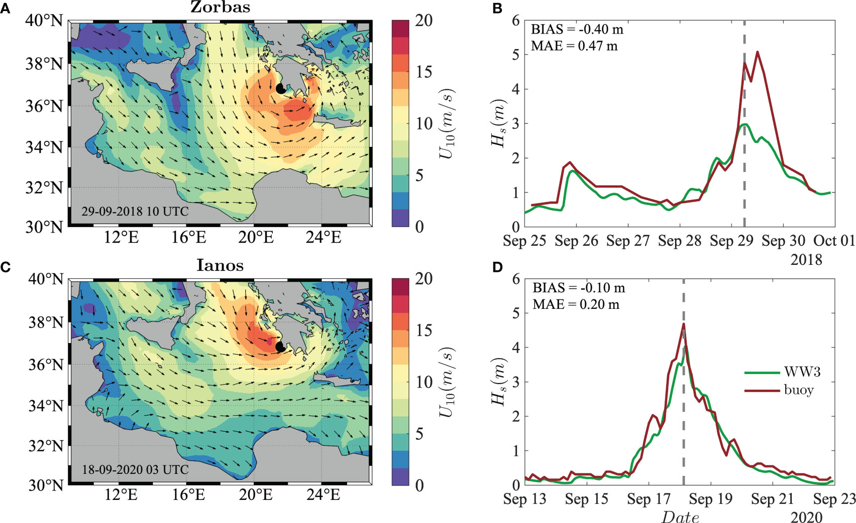
Figure 5 Comparison between model and buoy significant wave height H_s during Zorbas (A, B) and Ianos (C, D). (A, C) ERA5 near-surface (10-m height) wind speed U₁₀ (colored shading) and direction (arrows, decimated for graphical purposes) during peak time at the POSEIDON buoy location west of Pylos (black marker). (B, D) Significant wave height H_s at the Pylos buoy station from wave hindcast model (green line) and in-situ measurements (brown line). The time of peak model values is also shown (dashed grey line).

The maximum modelled significant wave height values at the Pylos station during Zorbas were reached on 29 September at 06 UTC (H_s around 3 m) and on 18 September at 03 UTC (H_s around 4 m) for Ianos. Interestingly, in the first case the wave model significantly underestimates the evolution of the wave field (BIAS = -0.40 m), whereas it captures the growth of Ianos more accurately (BIAS = -0.10 m), with only a slight temporal shift around the peak value. Although small shifts in the wind field due to the aforementioned coarseness of the atmospheric reanalysis could be responsible for significant differences in the wave field, the most likely reason for such discrepancy can be appreciated by looking at the wind fields at the time and location of the aforementioned events (Figures 5A, C). Indeed, during Zorbas, the surface wind around the buoy location was blowing offshore, with the cyclone eye almost centered around it, thereby leading to a strong underestimation of the wind speed, and therefore of the wave field, due to the orography effect (as already noted, among many, by Cavaleri and Bertotti, 2004; Barbariol et al., 2022). Conversely, the onshore winds around the buoy station during Ianos are not affected by the presence of nearby land and therefore produce more accurate wave fields, which match in-situ measurements.

Although our focus in the present work is on wave maxima, we note that the assessment of the modelled ${\overline{C}}_{max}$ can only be carried out indirectly, given the extremely limited number of observational platforms in the global oceans that are continuously collecting the wave elevation over a long time period, and in any case with different space and time domain sizes compared to the ones implemented herein. We therefore base our assessment of maximum crest heights on the performance of H_s shown above, since it represents the key parameter for determining the height of maximum expected individual crest heights (Benetazzo et al., 2021b).

3.3 Maximum individual waves

In this Section, we focus on the geographical pattern of the spatio-temporal maximum individual waves during the three MTLCs considered herein.

For this analysis, we first consider the extreme value statistics computed over a spatio-temporal domain Γ of fixed size (i.e., X, Y and D = constant) to give an overview of the geographical pattern and intensity of the expected value of second-order extreme crest heights ${\overline{C}}_{max}$. To this end, the hourly wave model outputs of the maximum individual crest heights computed directly using the space-time extreme WW3 model implementation are therefore used.

Since the choice of the size of the spatio-temporal volume over which to compute the extreme wave statistics is arbitrary and is usually driven only by the purpose of specific applications (see Benetazzo et al., 2021b), provided that the requirements of stationarity in time and homogeneity over space are satisfied, we consider a 3D region of size X = 100 m, Y = 100 m and D = 1200 s, which represents the typical horizontal footprint of an offshore platform and the typical duration of a wave buoy record. Results stemming from this analysis are shown in Figure 6.

Figure 6

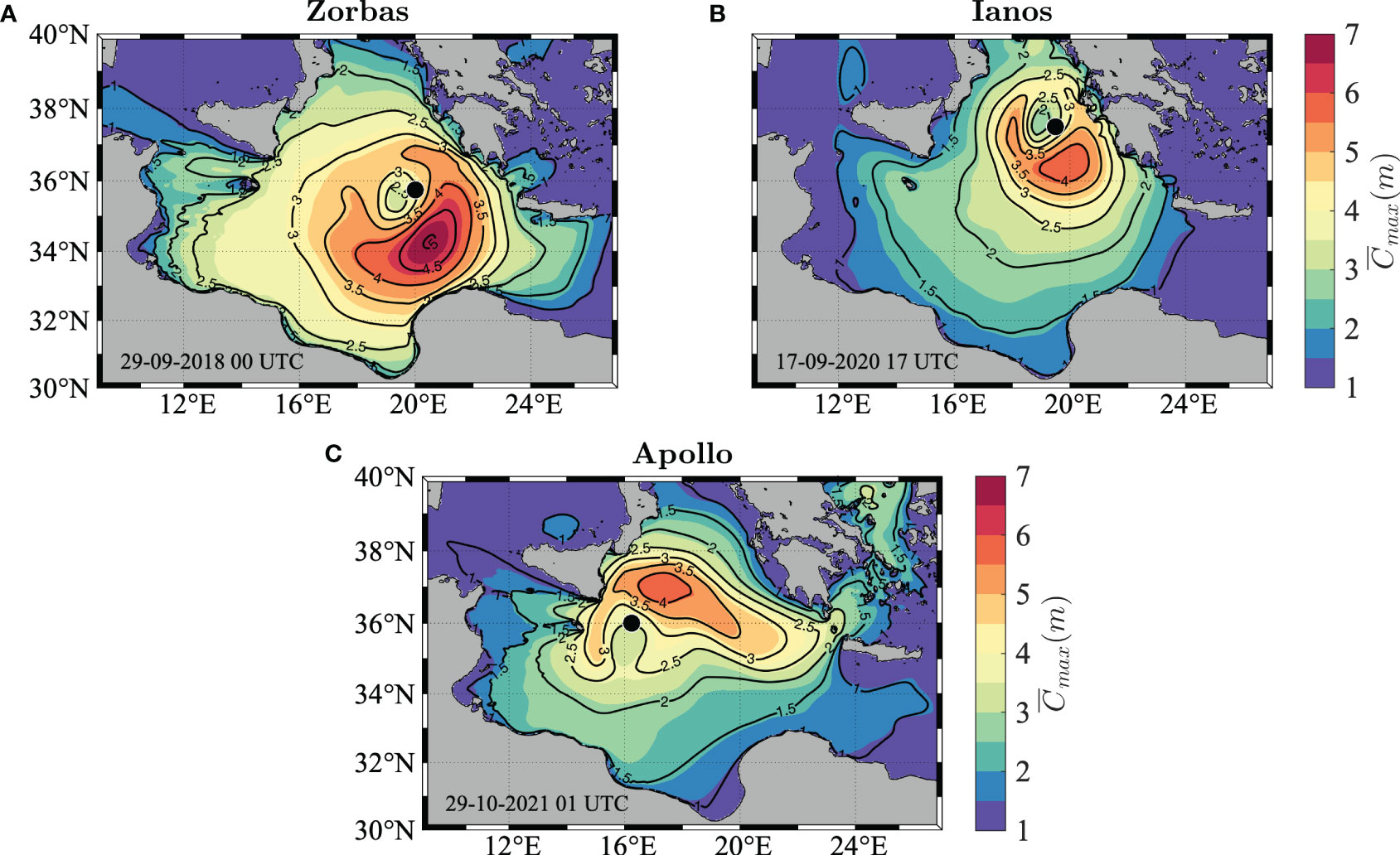
Figure 6 Maximum individual waves in the Ionian Sea during Zorbas (A), Ianos (B), and Apollo (C). Expected value of the maximum crest height (${\overline{C}}_{max}$) computed over a spatio-temporal domain of fixed size Γ: X = 100 m, Y = 100 m, D = 1200 s. Black contours show values of the significant wave height H_s, while the black marker indicates the position of the pressure minimum.

Once again, similarly to the case of a tropical cyclone (see Benetazzo et al., 2021a), the geographical pattern of ${\overline{C}}_{max}$ for Zorbas and Ianos is characterized by an asymmetry that mirrors the significant wave height (black contour lines), with the highest values located to the right of the cyclone as it moves along a southwest-to-northeast trajectory, while the pattern is slightly different for Apollo, due to the intense winds from the Peloponnese merging with the rotating wind field near the cyclone eye. In particular, values of ${\overline{C}}_{max}$ peaked at about 8 m for Zorbas on 29 September 2018 at 00 UTC, while Ianos on 17 September 2020 at 17 UTC and Apollo on 29 October 2021 at 01 UTC both displayed maximum expected crest heights around 6 m, which in the Ionian basin are usually considered to be extreme winter conditions (Barbariol et al., 2021).

The extreme value analysis is then carried out considering a sea state-dependent domain of variable size, which enables to highlight the sea regions where only the role of the 3D wave kinematics and steepness is dominant and prevents the normalized maxima ${\overline{C}}_{max}/H_s$ from reaching the highest values where the sample size is highest, i.e. in sea regions where young and short waves are present.

To this end, the dependence of ${\overline{C}}_{max}$ variability on (L_x, L_y, T_z) is removed by setting X, Y, D to be multiples of the sea state characteristics (see Equations 2–4). In particular, in the present study the domain size was set to include, on average, only one wave in the physical xy-space and 100 waves in time (X = L_x, Y = L_y, D = 100T_z).

Since the hourly wave model outputs over a domain of variable size are not available in the space-time extreme WW3 model implementation, for this type of analysis the second-order nonlinear approximation for ${\overline{C}}_{max}$ was computed using the directional wave spectra extracted at each grid point.

The normalized maximum expected crest height fields thus calculated over a sea state dependent domain are shown in Figure 7.

Figure 7

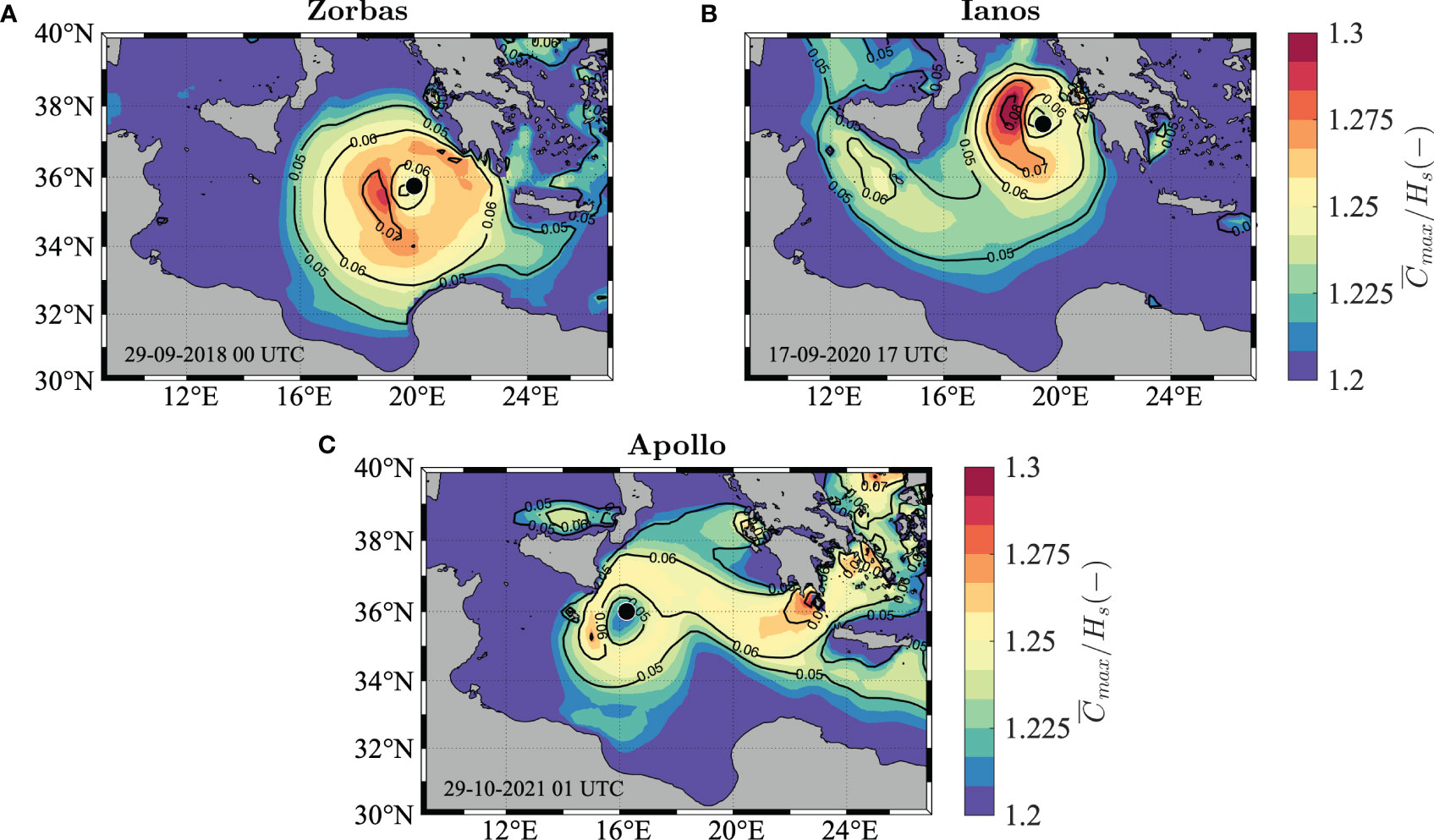
Figure 7 Maximum individual waves in the Ionian Sea during Zorbas (A), Ianos (B) and Apollo (C). Expected value of the maximum normalized crest height (${\overline{C}}_{max}/H_s$) computed over a spatio-temporal domain of variable size (sea state dependent) Γ: X = L_x, Y = L_y, D = 100T_z. Black contours show the bulk wave steepness μ, while the black marker indicates the position of the pressure minimum.

In this case the maximum crest heights follow the geographical pattern of the bulk wave steepness fields μ (black contour lines), with the largest values in the bottom-left quadrant of the cyclone, with respect to the cyclone track, where the wave field opposes somewhat the direction of the translating storm. Furthermore, in this quadrant the wave field is also more directionally spread (not shown here, see Mori, 2012 and Benetazzo et al., 2021a for the case of a TC), which affects the irregularity parameters of Equations 2, 3, thus contributing to the increase of the maximum expected crest height values.

For Zorbas and Ianos, in particular, the enhancement of crest heights by second-order nonlinearities (bulk wave steepness above 0.07) leads to ${\overline{C}}_{max}/H_s$ values up to 1.29 and 1.32, respectively. On the other hand, Apollo displays the highest normalized maxima off the Peloponnesian coast (${\overline{C}}_{max}/H_s$ around 1.27), where strong winds and younger sea states are present, as well as in a very limited region in the bottom-left sector of the storm (${\overline{C}}_{max}/H_s$ around 1.26), partly affected by the presence of land to the west.

3.4 Influence of crossing sea states

So far, we have analysed the spatial distribution of the maximum individual waves around the eye of the three Medicane events selected for this study, regardless of whether they are characterized by a single wind sea wave system or by a combination of a wind sea and a swell. In this Section, we investigate the characteristics of the wave fields within the three cyclones and we investigate how the resulting crossing sea conditions affect the generation of maximum waves compared to the analysis carried out in the previous Section.

To characterize the geographical regions where both a wind sea and a swell are present at the same time, the spatial fields of the crossing sea parameters SSER, ID and $\Delta \theta$ (see Equations 6-8) are displayed in Figure 8 during peak conditions. We note that, since our interest is mainly in the highest waves around the cyclone eye, to avoid uncertainties in the computation of the spectral parameters we used a threshold of H_s = 1 m for the identification of each partition.

Figure 8

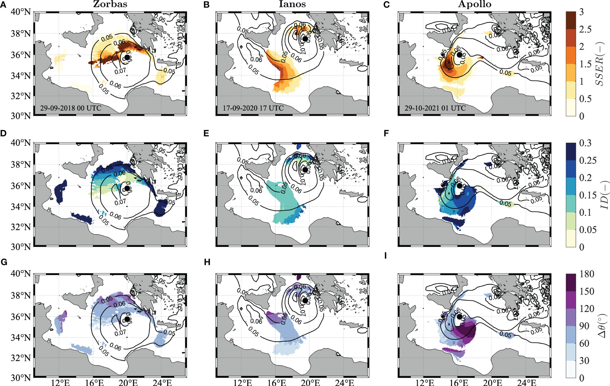
Figure 8 Crossing sea parameters derived from the first two partitions of wave model spectra in the Ionian Sea during Zorbas (A, D, G), Ianos (B, E, H) and Apollo (C, F, I). Sea-Swell Equivalent Ratio (SSER, A-C), Intermodal Distance (ID, D-F) and crossing angle ($\Delta \theta$, G-I) are shown (colored shading). For reference, black contours of the bulk wave steepness μ are displayed, while the black marker indicates the position of the pressure minimum.

In line with the work by Mori (2012), for all three events unimodal sea states (white areas in Figure 8) occur mainly to the right of the cyclone eye with respect to the direction of propagation of the storm (see Figure 2 for the cyclone tracks), while crossing sea states (colored areas in Figure 8) are confined in the left sectors of the MTLC, where the swell generated at an earlier stage intercepts the local wind sea.

As regards the energy ratio (Figures 8A-C), the wind sea contribution is dominant (SSER > 1) close to the eye, while swell-dominated areas (SSER< 1) are present mostly in the outer crossing sea regions. Compared to Zorbas and Apollo, however, Ianos displays an additional area where both wind sea and swell are present, which is located outside the main area affected by the cyclone, between Sicily and Libya, where a wind sea caused by the southeasterly winds blowing through the Sicily Strait meets a swell propagating out of the main cyclone field.

The geographical pattern of the peak frequency separation between wind sea and swell for all three events (Figures 8D-F) shows that wind sea-dominated areas are usually characterized by smaller ID values, due to the similar wavelengths of wind sea and swell, while large ID values are more common in the outer, swell-dominated sectors.

Conversely, the relative crossing angle $\text{Δ}\theta$ (Figures 8G-I) displays different patterns for each event due to the different ground structure of the wind field. In general, orthogonal crossing conditions ($\text{Δ}\theta$ around 90°) are present in the left sectors of all three cyclones, while following conditions ($\text{Δ}\theta$ around 0°) are found in the top-left and bottom-left regions of Zorbas, north of Lybia outside the wave field around the eye during Ianos and in the top-left quadrant of the cyclone during Apollo. Moreover, opposing conditions ($\text{Δ}\theta$ around 180°) cover a significant portion of the cyclone field only during Apollo, in the bottom-left quadrant, as a result of the strong swell wave field generated by the strong winds south of the Peloponnese crossing the rotating wind sea field south of Sicily.

Compared to the results obtained using the bulk wave steepness parameter $\mu$ of Equation (5) (Figure 7), the crossing sea regions highlighted above seem to partly overlap with the geographical areas where the highest values of normalized maximum expected crest heights were found, especially in the case of Zorbas and Apollo.

Since the short-scale interaction of concurrent wind sea and swell may be one of the mechanisms at play in the generation of extreme crest heights during MTLC events, as previously suggested in the case of tropical cyclones (see Benetazzo et al., 2021a and Davison et al., 2022), to improve the description of the spatial pattern of ${\overline{C}}_{max}/H_s$ by also accounting for such interactions between the two wave systems, we compute the expected value of the individual highest waves over a variable domain (X = L_x, Y = L_y, D = 100T_z) employing the second-order nonlinear spatio-temporal distribution of Equation 1 based on the crossing sea steepness parameter ${\mu }_{crossing}$ of Equation 9.

Once again, since the wave model outputs over a domain of variable size are not available in the space-time extreme WW3 model implementation, for this analysis we relied on the directional wave spectra extracted at each grid point.

The resulting large-scale spatio-temporal crest height statistics, expressed in terms of their ratio with respect to the maximum expected crest heights obtained using the bulk wave steepness (${\overline{C}}_{max,crossing}/{\overline{C}}_{max}$), are shown in Figure 9.

Figure 9

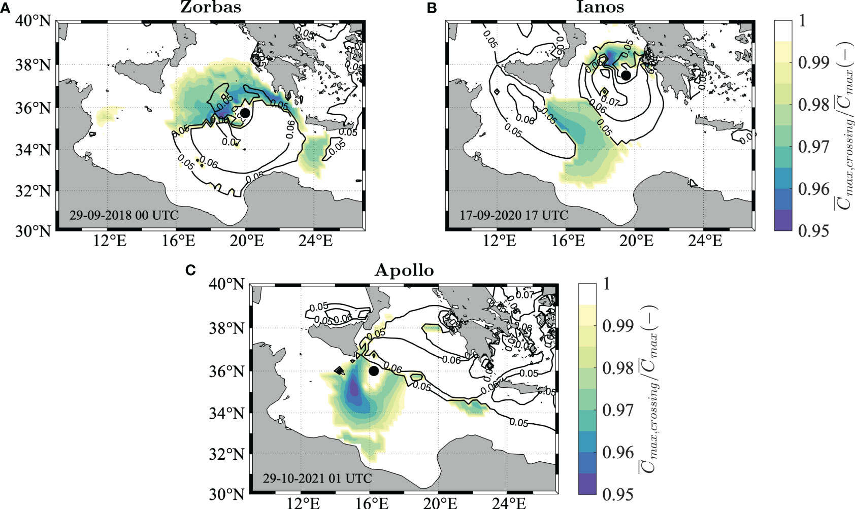
Figure 9 Maximum individual waves in the Ionian Sea during Zorbas (A), Ianos (B) and Apollo (C). Ratio between the maximum expected crest heights (C̄_max,crossing/C̄_max) based on two different steepness parametrizations (μ_crossing and μ) computed over a spatio-temporal domain of variable size (sea state dependent): X = L_x, Y = L_y, D = 100T_z. The black marker indicates the position of the pressure minimum and black contours show the crossing wave steepness μ_crossing..

Following Equation 9, the value of ${\mu }_{crossing}$ is influenced by the second-order sum and difference interaction terms, which are highest for particularly small or large crossing angles and, to a lesser extent, for large ID values (see Figure 1). In the MTCLs considered herein, the strongest wave-wave interactions therefore occur in the top-left and bottom-left sectors of Zorbas and in the lower crossing sea region North of Lybia during Ianos ($\Delta \theta$ between 30 and 60° for both cases in Figure 8), as well as in the bottom-left region of the cyclone field during Apollo (ID above 0.2 and $\Delta \theta$ above 150°). However, depending on the spatial position with respect to the cyclone eye, their effect may be overshadowed by the influence of the local wavenumbers of swell and wind sea [first and second terms on the right-hand side of Equation 5] and by the local value of SSER (Figures 8A-C). The resulting pattern of ${\mu }_{crossing}$ (black contours in Figure 9) is therefore rather complex and more spatially variable than the bulk wave steepness.

As a result, given the upper bounded nature of Equation 5, the geographical pattern of the ratio between ${\overline{C}}_{max,crossing}$ and ${\overline{C}}_{max}$ (color shading in Figure 9) displays the largest values (close to unity) for following and opposing conditions, and over swell-dominated areas (large ID values), for which the effect of crossing angle on the strength of the wave-wave interactions is more limited and the contribution of the wind sea wavenumber is non negligible. Conversely, for wind sea-dominated regions (low ID values), where the influence of crossing angle on the strength of the interactions is largest, standard unidirectional predictions of ${\overline{C}}_{max}$ overestimate maximum expected crest height values in orthogonal conditions (up to 5%).

Overall, since the largest expected maximum crest heights of Figure 7 are mainly found either in pure wind seas or in wind sea-dominated, orthogonal crossing conditions for the three Medicanes analyzed herein, our results indicate that the interaction of wind sea and swell is marginally responsible for the highest waves thus found near the cyclone eye.

It must be noted that the estimates of C̄_max,crossing obtained herein present several sources of uncertainty, which deserve further investigation. Indeed, in the computation of maximum expected crest heights we have neglected the effect of directional spreading of the individual wave systems, which was shown to mask the crossing angle contribution in the exceedance probabilities (Luxmoore et al., 2019). Additionally, the irregularity parameters of Equations 2, 3 were computed by considering the total directional wave spectrum rather than the single spectral partitions. Furthermore, the second-order interaction kernels in the crossing wave steepness formulation of Equation 9 were found to be very sensitive to the type of frequencies and directions considered for their computation, with mean quantities yielding significantly larger values than the peak quantities used in this work.

Lastly, due to the spatially and temporally limited wave fields, especially in the case of Zorbas and Ianos, we expect the underestimation of coastal winds in the ERA5 reanalysis dataset (see Barbariol et al., 2022; Benetazzo et al., 2022; Campos et al., 2022), also found in the wave model assessment at the Pylos station (Figure 5), to affect estimates of the crossing sea parameters near the coastal areas.

To avoid at least part of the aforementioned shortcomings, simulations with a higher spatial resolution of the atmospheric forcing should be performed and directional spreading effects should be included in the wave steepness formulation.

4 Conclusions

In this paper, we have carried out a spectral wave model hindcast forced by ERA5 atmospheric reanalysis winds to characterize the large-scale spatial distribution of maximum individual waves (crest heights) associated with selected tropical-like cyclone events in the Mediterranean Sea, namely Zorbas in 2018, Ianos in 2020 and Apollo in 2021. The subject has been discussed in previous studies only for the case of tropical cyclones, while few studies have focused on the waves generated during tropical-like cyclones, with no firm conclusion on the magnitude and spatial pattern of maximum individual waves.

For the assessment of the modelled significant wave height fields, we have used both in-situ and altimeter measurements. While the comparison with altimeter data is generally good, the comparison with buoy observations offshore Greece is strongly affected by the underestimation of ERA5 coastal winds, in line with previous findings.

In general, apart from the shorter lifespan of MTLC events and their greater proximity to land, which somewhat limits the wave field growth, the spatial distribution of maximum individual waves within a tropical-like cyclone is similar to the case of tropical cyclones: the maximum expected crest heights mirror the asymmetry of the significant wave height due to the extended fetch effect, while the steepest waves are located in the bottom-left quadrants of the translating storm. In particular, of the Medicane events studied in this work, Zorbas displayed the highest values of ${\overline{C}}_{max}$, which were estimated at 8 m, while the steepest waves were recorded during Ianos, where values above ${\overline{C}}_{max}/H_s=$ 1.3 were reached.

To quantify the role of the interacting wind sea and swell fields in the generation of such high waves, the present work advances previous investigations by carrying out a spectral partitioning of the cyclone wave field and computing the maximum expected crest heights with a novel formulation of the wave steepness which accounts for the local crossing conditions. Our results show large regions of crossing seas in the left sectors of all three Medicanes, whose effect on the generation of the highest crest heights thus found however is confined, since the largest waves occur either in pure wind seas or in wind sea-dominated orthogonal crossing conditions, for which the second-order nonlinear interactions between the two wave systems are weak. In these crossing conditions, the bulk steepness parameter overestimates the largest waves by up to 5%.

We note, however, that the estimates for crossing seas derived in this work might be affected by some degree of approximation in the formulations employed and by the significant underestimation of the wind dataset used, especially near the coast. Therefore, while dedicated, fully coupled numerical models would grant a significant improvement in the simulation of the cyclone wave field, future analyses with the present modelling approach should include a comparison of modelled wave maxima with phase-resolving spatio-temporal measurements, in order to assess the accuracy of the geographical patterns obtained herein. Notwithstanding, we stress the overall importance of considering crossing sea parameters, as well as the spectral characteristics of the constituent wave systems, to obtain a more realistic description of the highest individual waves during both tropical and tropical-like cyclones.

Data availability statement

The raw data supporting the conclusions of this article will be made available by the authors, without undue reservation.

Author contributions

SD: Conceptualization, Data curation, Formal analysis, Investigation, Methodology, Software, Validation, Writing – original draft, Writing – review & editing. AB: Funding acquisition, Project administration, Resources, Supervision, Visualization, Writing – review & editing. FB: Funding acquisition, Project administration, Resources, Software, Supervision, Visualization, Writing – review & editing. AR: Investigation, Resources, Supervision, Visualization, Writing – review & editing. RF: Resources, Visualization, Writing – review & editing.

Funding

The author(s) declare financial support was received for the research, authorship, and/or publication of this article. This research was supported by the Korea Institute of Marine Science & Technology Promotion (KIMST) funded by the Ministry of Oceans and Fisheries (20210607). This work was partly developed in the framework of the National Centre for HPC, Big Data and Quantum Computing - PNRR Project, funded by the European Union - Next Generation EU, and was partly supported by the Special Project ASIM-CPL, funded by ECMWF, and by the PON - DM1062 Project.

Acknowledgments

We are grateful to Luigi Cavaleri (CNR-ISMAR) for the stimulating and useful discussions on wave modelling.

Conflict of interest

The authors declare that the research was conducted in the absence of any commercial or financial relationships that could be construed as a potential conflict of interest.

The author(s) declared that they were an editorial board member of Frontiers, at the time of submission. This had no impact on the peer review process and the final decision.

Publisher’s note

All claims expressed in this article are solely those of the authors and do not necessarily represent those of their affiliated organizations, or those of the publisher, the editors and the reviewers. Any product that may be evaluated in this article, or claim that may be made by its manufacturer, is not guaranteed or endorsed by the publisher.

References

Abdolali A., van der Westhuysen A., Ma Z., Mehra A., Roland A., Moghimi S. (2021). Evaluating the accuracy and uncertainty of atmospheric and wave model hindcasts during severe events using model ensembles. Ocean Dyn 71, 217–235. doi: 10.1007/s10236-020-01426-9

CrossRef Full Text | Google Scholar

Adcock T. A. A., Taylor P. H., Yan S., Ma Q. W., Janssen P. A. E. M. (2011). Did the Draupner wave occur in a crossing sea? Proceedingis R. Soc. A 467, 1–18. doi: 10.1098/rspa.2011.0049

CrossRef Full Text | Google Scholar

Ardhuin F., Rogers E., Babanin A., Filipot J.-F., Magne R., Roland A., et al. (2010). Semiempirical dissipation source functions for ocean waves. Part I: definition, calibration, and validation. J. Phys. Oceanogr 40, 1917–1941. doi: 10.1175/2010JPO4324.1

CrossRef Full Text | Google Scholar

Barbariol F., Alves J. H. G. M., Benetazzo A., Bergamasco F., Bertotti L., Carniel S., et al. (2017). Numerical modeling of space-time wave extremes using WAVEWATCH III. Ocean Dyn 67, 535–549. doi: 10.1007/s10236-016-1025-0

CrossRef Full Text | Google Scholar

Barbariol F., Davison S., Falcieri F. M., Ferretti R., Ricchi A., Sclavo M., et al. (2021). Wind waves in the mediterranean sea: an ERA5 reanalysis wind-based climatology. Front. Mar. Sci. 8. doi: 10.3389/fmars.2021.760614

CrossRef Full Text | Google Scholar

Barbariol F., Pezzutto P., Davison S., Bertotti L., Cavaleri L., Papa A., et al. (2022). Wind-wave forecasting in enclosed basins using statistically downscaled global wind forcing. Front. Mar. Sci. 9. doi: 10.3389/fmars.2022.1002786

PubMed Abstract | CrossRef Full Text | Google Scholar

Baxevani A., Rychlik I. (2006). Maxima for gaussian seas. Ocean Eng. 33, 895–911. doi: 10.1016/j.oceaneng.2005.06.006

CrossRef Full Text | Google Scholar

Benetazzo A., Barbariol F., Bergamasco F., Bertotti L., Yoo J., Shim J.-S., et al. (2021a). On the extreme value statistics of spatio-temporal maximum sea waves under cyclone winds. Prog. Oceanogr 197, 102642. doi: 10.1016/j.pocean.2021.102642

CrossRef Full Text | Google Scholar

Benetazzo A., Barbariol F., Bergamasco F., Torsello A., Carniel S., Sclavo M. (2015). Observation of extreme sea waves in a space-time ensemble. J. Phys. Oceanogr 45, 2261–2275. doi: 10.1175/JPO-D-15-0017.1

CrossRef Full Text | Google Scholar

Benetazzo A., Barbariol F., Pezzutto P., Staneva J., Behrens A., Davison S., et al. (2021b). Towards a unified framework for extreme sea waves from spectral models: rationale and applications. Ocean Eng. 219, 108263. doi: 10.1016/j.oceaneng.2020.108263

CrossRef Full Text | Google Scholar

Benetazzo A., Davison S., Barbariol F., Mercogliano P., Favaretto C., Sclavo M. (2022). Correction of ERA5 wind for regional climate projections of sea waves. Water (Basel) 14, 1590. doi: 10.3390/w14101590

CrossRef Full Text | Google Scholar

Black P. G., D’Asaro E. A., Drennan W. M., French J. R., Niiler P. P., Sanford T. B., et al. (2007). Air–sea exchange in hurricanes: synthesis of observations from the coupled boundary layer air–sea transfer experiment. Bull. Am. Meteorol Soc. 88, 357–374. doi: 10.1175/BAMS-88-3-357

CrossRef Full Text | Google Scholar

Borzì A. M., Minio V., Cannavò F., Cavallaro A., D’Amico S., Gauci A., et al. (2022). Monitoring extreme meteo-marine events in the Mediterranean area using the microseism (Medicane Apollo case study). Sci. Rep. 12, 21363. doi: 10.1038/s41598-022-25395-9

PubMed Abstract | CrossRef Full Text | Google Scholar

Brennan J., Dudley J. M., Dias F. (2018). Extreme waves in crossing sea states. Int. J. Ocean Coast. Eng. 01, 1850001. doi: 10.1142/S252980701850001X

CrossRef Full Text | Google Scholar

Campos R. M., Gramcianinov C. B., de Camargo R., a Silva Dias P. L. (2022). Assessment and calibration of ERA5 severe winds in the atlantic ocean using satellite data. Remote Sens (Basel) 14, 4918. doi: 10.3390/rs14194918

CrossRef Full Text | Google Scholar

Cavaleri L., Bertotti L. (2004). Accuracy of the modelled wind and wave fields in enclosed seas. Tellus A 56, 167–175. doi: 10.3402/tellusa.v56i2.14398

CrossRef Full Text | Google Scholar

Cavicchia L., von Storch H., Gualdi S. (2014). Mediterranean tropical-like cyclones in present and future climate. J. Clim 27, 7493–7501. doi: 10.1175/JCLI-D-14-00339.1

CrossRef Full Text | Google Scholar

Christou M. A., Tromans P. S., Vanderschuren L., Ewans K. (2009). “Second-order crest statistics of realistic sea states,” in Proceedings of the 11th international workshop on wave hindcasting and forecasting, Halifax, Canada(Halifax, Canada). Available at: https://api.semanticscholar.org/CorpusID:212724034.

Google Scholar

Dalzell J. F. (1999). A note on finite depth second-order wave–wave interactions. Appl. Ocean Res. 21, 105–111. doi: 10.1016/S0141-1187(99)00008-5

CrossRef Full Text | Google Scholar

Davison S., Benetazzo A., Barbariol F., Ducrozet G., Yoo J., Marani M. (2022). Space-time statistics of extreme ocean waves in crossing sea states. Front. Mar. Sci. 9. doi: 10.3389/fmars.2022.1002806

PubMed Abstract | CrossRef Full Text | Google Scholar

Donelan M. A., Drennan W. M., Katsaros K. B. (1997). The air–sea momentum flux in conditions of wind sea and swell. J. Phys. Oceanogr 27, 2087–2099. doi: 10.1175/1520-0485(1997)027<2087:TASMFI>2.0.CO;2

CrossRef Full Text | Google Scholar

Efimov V. V., Stanichnyi S. V., Shokurov M. V., Yarovaya D. A. (2008). Observations of a quasi-tropical cyclone over the Black Sea. Russian Meteorology Hydrology 33, 233–239. doi: 10.3103/S1068373908040067

CrossRef Full Text | Google Scholar

Emanuel K. (2005). Genesis and maintenance of &quot;Mediterranean hurricanes&quot;. Adv. Geosciences 2, 217–220. doi: 10.5194/adgeo-2-217-2005

CrossRef Full Text | Google Scholar

Fedele F. (2012). Space–time extremes in short-crested storm seas. J. Phys. Oceanogr 42, 1601–1615. doi: 10.1175/JPO-D-11-0179.1

CrossRef Full Text | Google Scholar

Fedele F., Brennan J., de León S. P., Dudley J., Dias F. (2016). Real world ocean rogue waves explained without the modulational instability. Sci. Rep. 6, 1–11. doi: 10.1038/srep27715

PubMed Abstract | CrossRef Full Text | Google Scholar

Fedele F., Lugni C., Chawla A. (2017). The sinking of the El Faro : predicting real world rogue waves during Hurricane Joaquin. Sci. Rep. 7, 11188. doi: 10.1038/s41598-017-11505-5

PubMed Abstract | CrossRef Full Text | Google Scholar

Fedele F., Tayfun M. A. (2009). On nonlinear wave groups and crest statistics. J. Fluid Mech. 620, 221–239. doi: 10.1017/S0022112008004424

CrossRef Full Text | Google Scholar

Ferrarin C., Pantillon F., Davolio S., Bajo M., Miglietta M. M., Avolio E., et al. (2023). Assessing the coastal hazard of Medicane Ianos through ensemble modelling. Natural Hazards Earth System Sci. 23, 2273–2287. doi: 10.5194/nhess-23-2273-2023

CrossRef Full Text | Google Scholar

Figa-Saldaña J., Wilson J. J. W., Attema E., Gelsthorpe R., Drinkwater M. R., Stoffelen A. (2002). The advanced scatterometer (ASCAT) on the meteorological operational (MetOp) platform: A follow on for European wind scatterometers. Can. J. Remote Sens. 28, 404–412. doi: 10.5589/m02-035

CrossRef Full Text | Google Scholar

Forristall G. Z. (2000). Wave crest distributions: observations and second-order theory. J. Phys. Oceanogr 30, 1931–1943. doi: 10.1175/1520-0485(2000)030<1931:WCDOAS>2.0.CO;2

CrossRef Full Text | Google Scholar

Franklin J. L., Pasch R. J., Avila L. A., Beven J. L., Lawrence M. B., Stewart S. R., et al. (2006). Atlantic hurricane season of 2004. Mon Weather Rev. 134, 981–1025. doi: 10.1175/MWR3096.1

CrossRef Full Text | Google Scholar

González-Alemán J. J., Pascale S., Gutierrez-Fernandez J., Murakami H., Gaertner M. A., Vecchi G. A. (2019). Potential increase in hazard from mediterranean hurricane activity with global warming. Geophys Res. Lett. 46, 1754–1764. doi: 10.1029/2018GL081253

CrossRef Full Text | Google Scholar

Guedes Soares C., Carvalho A. N. (2003). Probability distributions of wave heights and periods in measured combined sea-states from the Portuguese coast. J. Offshore Mechanics Arctic Eng. 125, 198–204. doi: 10.1115/1.1576816

CrossRef Full Text | Google Scholar

Hanson J. L., Phillips O. M. (2001). Automated analysis of ocean surface directional wave spectra. J. Atmos Ocean Technol. 18, 277–293. doi: 10.1175/1520-0426(2001)018<0277:AAOOSD>2.0.CO;2

CrossRef Full Text | Google Scholar

Hasselmann S., Hasselmann K., Allender J. H., Barnet T. P. (1985). Computations and parameterizations of the nonlinear energy transfer in a gravity-wave specturm. Part II: parameterizations of the nonlinear energy transfer for application in wave models. J. Phys. Oceanogr 15, 1378–1391. doi: 10.1175/1520-0485(1985)015<1378:CAPOTN>2.0.CO;2

CrossRef Full Text | Google Scholar

Hersbach H., Bell B., Berrisford P., Hirahara S., Horányi A., Muñoz-Sabater J., et al. (2020). The ERA5 global reanalysis. Q. J. R. Meteorological Soc. 146, 1999–2049. doi: 10.1002/qj.3803

CrossRef Full Text | Google Scholar

Holthuijsen L. H., Powell M. D., Pietrzak J. D. (2012). Wind and waves in extreme hurricanes. J. Geophys Res. Oceans 117, C09003 10–15. doi: 10.1029/2012JC007983

CrossRef Full Text | Google Scholar

Hu K., Chen Q. (2011). Directional spectra of hurricane-generated waves in the Gulf of Mexico. Geophys Res. Lett. 38, L19608. doi: 10.1029/2011GL049145

CrossRef Full Text | Google Scholar

Jiang X., Guan C., Wang D. (2019). Rogue waves during Typhoon Trami in the East China Sea. J. Oceanol Limnol 37, 1817–1836. doi: 10.1007/s00343-019-8256-0

CrossRef Full Text | Google Scholar

Kanehira T., McAllister M. L., Draycott S., Nakashima T., Taniguchi N., Ingram D. M., et al. (2021). Highly directionally spread, overturning breaking waves modelled with Smoothed Particle Hydrodynamics: A case study involving the Draupner wave. Ocean Model. (Oxf) 164, 101822. doi: 10.1016/j.ocemod.2021.101822

CrossRef Full Text | Google Scholar

Lagouvardos K., Karagiannidis A., Dafis S., Kalimeris A., Kotroni V. (2022). Ianos—A hurricane in the mediterranean. Bull. Am. Meteorol Soc. 103, E1621–E1636. doi: 10.1175/BAMS-D-20-0274.1

CrossRef Full Text | Google Scholar

Liu Q., Babanin A., Fan Y., Zieger S., Guan C., Moon I.-J. (2017). Numerical simulations of ocean surface waves under hurricane conditions: Assessment of existing model performance. Ocean Model. (Oxf) 118, 73–93. doi: 10.1016/j.ocemod.2017.08.005

CrossRef Full Text | Google Scholar

Longuet-Higgins M. S. (1963). The effect of nonlinearities on statistical distribution in the theory of sea waves. J. Fluid Mech. 17, 459–480. doi: 10.1017/S0022112063001452

CrossRef Full Text | Google Scholar

Longuet-Higgins M. S. (1975). On the joint distribution of the periods and amplitudes of sea waves. J. Geophys Res. 80, 2688–2694. doi: 10.1029/JC080i018p02688

CrossRef Full Text | Google Scholar

Luxmoore J. F., Ilic S., Mori N. (2019). On kurtosis and extreme waves in crossing directional seas: a laboratory experiment. J. Fluid Mech. 876, 792–817. doi: 10.1017/jfm.2019.575

CrossRef Full Text | Google Scholar

McAllister M. L., Adcock T. A. A., Taylor P. H., van den Bremer T. S. (2018). The set-down and set-up of directionally spread and crossing surface gravity wave groups. J. Fluid Mech. 835, 131–169. doi: 10.1017/jfm.2017.774

CrossRef Full Text | Google Scholar

McAllister M. L., Adcock T. A. A., Taylor P. H., van den Bremer T. S. (2019). A note on the second-order contribution to extreme waves generated during hurricanes. J. Offshore Mechanics Arctic Eng. 141, 1–10. doi: 10.1115/1.4042540

CrossRef Full Text | Google Scholar

McAllister M. L., van den Bremer T. S. (2019). Lagrangian measurement of steep directionally spread ocean waves: second-order motion of a wave-following measurement buoy. J. Phys. Oceanogr 49, 3087–3108. doi: 10.1175/JPO-D-19-0170.1

CrossRef Full Text | Google Scholar

Moon I. J., Ginis I., Hara T., Tolman H. L., Wright C. W., Walsh E. J. (2003). Numerical simulation of sea surface directional wave spectra under hurricane wind forcing. J. Phys. Oceanogr. 33, 1680–1706. doi: 10.1175/2410.1

CrossRef Full Text | Google Scholar

Mori N. (2012). Freak waves under typhoon conditions. J. Geophys Res. Oceans 117, 1–12. doi: 10.1029/2011JC007788

CrossRef Full Text | Google Scholar

Onorato M., Waseda T., Toffoli A., Cavaleri O., Gramstad A., Janssen P. A. E. M., et al (2009). Statistical properties of directional ocean waves: the role of the modulational instability in the formation of extreme events. Phys. Rev. Lett. 102, 114502. doi: 10.1103/PhysRevLett.102.114502

PubMed Abstract | CrossRef Full Text | Google Scholar

Patlakas P., Stathopoulos C., Tsalis C., Kallos G. (2021). Wind and wave extremes associated with tropical-like cyclones in the Mediterranean basin. Int. J. Climatology 41 (Suppl. 1): E1623–E1644. doi: 10.1002/joc.6795

CrossRef Full Text | Google Scholar

Petrova P. G., Guedes Soares C. (2009). Probability distributions of wave heights in bimodal seas in an offshore basin. Appl. Ocean Res. 31, 90–100. doi: 10.1016/j.apor.2009.06.005

CrossRef Full Text | Google Scholar

Portilla J., Caicedo A. L., Padilla-Hernández R., Cavaleri L. (2015). Spectral wave conditions in the Colombian Pacific Ocean. Ocean Model. (Oxf) 92, 149–168. doi: 10.1016/j.ocemod.2015.06.005

CrossRef Full Text | Google Scholar

Pytharoulis I., Kartsios S., Tegoulias I., Feidas H., Miglietta M., Matsangouras I., et al. (2018). Sensitivity of a mediterranean tropical-like cyclone to physical parameterizations. Atmosphere (Basel) 9, 436. doi: 10.3390/atmos9110436

CrossRef Full Text | Google Scholar

Ribal A., Young I. R. (2019). 33 years of globally calibrated wave height and wind speed data based on altimeter observations. Sci. Data 6, 77. doi: 10.1038/s41597-019-0083-9

PubMed Abstract | CrossRef Full Text | Google Scholar

Ricchi A., Miglietta M. M., Bonaldo D., Cioni G., Rizza U., Carniel S. (2019). Multi-physics ensemble versus atmosphere–ocean coupled model simulations for a tropical-like cyclone in the mediterranean sea. Atmosphere (Basel) 10, 202. doi: 10.3390/atmos10040202

CrossRef Full Text | Google Scholar

Rodriguez G., Soares C. G., Pacheco M., Pe´rez-Martell E. (2002). Wave height distribution in mixed sea states. J. Offshore Mechanics Arctic Eng. 124, 34–40. doi: 10.1115/1.1445794

CrossRef Full Text | Google Scholar

Sharma J. N., Dean R. G. (1979). Development and evaluation of a procedure for simulating a random directional second order sea surface and associated wave forces. Ocean Engineering Rep. 20 (University of Delaware), 112 pp.

Google Scholar

Støle-Hentschel S., Trulsen K., Nieto Borge J. C., Olluri S. (2020). Extreme wave statistics in combined and partitioned windsea and swell. Water Waves 2, 169–184. doi: 10.1007/s42286-020-00026-w

CrossRef Full Text | Google Scholar

Tayfun M. A. (1980). Narrow-band nonlinear sea waves. J. Geophys Res. 85, 1548–1552. doi: 10.1029/JC085iC03p01548

CrossRef Full Text | Google Scholar

Tayfun M. A. (2006). Statistics of nonlinear wave crests and groups. Ocean Eng. 33, 1589–1622. doi: 10.1016/j.oceaneng.2005.10.007

CrossRef Full Text | Google Scholar

Toffoli A., Onorato M., Monbaliu J. (2006). Wave statistics in unimodal and bimodal seas from a second-order model. Eur. J. Mechanics - B/Fluids 25, 649–661. doi: 10.1016/j.euromechflu.2006.01.003

CrossRef Full Text | Google Scholar

Tous M., Zappa G., Romero R., Shaffrey L., Vidale P. L. (2016). Projected changes in medicanes in the HadGEM3 N512 high-resolution global climate model. Clim Dyn 47, 1913–1924. doi: 10.1007/s00382-015-2941-2

CrossRef Full Text | Google Scholar

Trulsen K., Nieto Borge J. C., Gramstad O., Aouf L., Lefèvre J. (2015). Crossing sea state and rogue wave probability during the Prestige accident. J. Geophys Res. Oceans 120, 7113–7136. doi: 10.1002/2015JC011161

CrossRef Full Text | Google Scholar

Varlas G., Vervatis V., Spyrou C., Papadopoulou E., Papadopoulos A., Katsafados P. (2020). Investigating the impact of atmosphere–wave–ocean interactions on a Mediterranean tropical-like cyclone. Ocean Model. (Oxf) 153, 101675. doi: 10.1016/j.ocemod.2020.101675

CrossRef Full Text | Google Scholar

Waseda T., Kinoshita T., Tamura H. (2009). Evolution of a random directional wave and freak wave occurrence. J. Phys. Oceanogr 39, 621–639. doi: 10.1175/2008JPO4031.1

CrossRef Full Text | Google Scholar

Wright C. W., Walsh E. J., Vandemark D., Krabill W. B., Garcia A. W., Houston S. H., et al. (2001). Hurricane directional wave spectrum spatial variation in the open ocean. J. Phys. Oceanogr 31, 2472–2488. doi: 10.1175/1520-0485(2001)031<2472:HDWSSV>2.0.CO;2

CrossRef Full Text | Google Scholar

WW3DG (2019). The WAVEWATCH III^® Development Group (WW3DG), 2019: User man- ual and system documentation of WAVEWATCH III version 6.07. Tech. Note 333, NOAA/NWS/NCEP/MMAB (College Park, MD, USA), 465 pp. + Appendices.

Google Scholar

Young I. R. (2003). A review of the sea state generated by hurricanes. Mar. Structures 16, 201–218. doi: 10.1016/S0951-8339(02)00054-0

CrossRef Full Text | Google Scholar

Young I. (2017). A review of parametric descriptions of tropical cyclone wind-wave generation. Atmosphere (Basel) 8, 194. doi: 10.3390/atmos8100194

CrossRef Full Text | Google Scholar

Young I. R., Ribal A. (2019). Multiplatform evaluation of global trends in wind speed and wave height. Sci. (1979) 364, 548–552. doi: 10.1126/science.aav9527

CrossRef Full Text | Google Scholar