Tidal energy extraction modifies tidal asymmetry and transport in a shallow, well-mixed estuary

Tidal energy extraction is increasingly being studied as a potential renewable energy resource in estuaries worldwide. Although it is understood that energy extraction via tidal stream turbines can modify currents and transport within estuaries, it is not clear how the underlying nonlinear physical mechanisms dictating tidal hydrodynamics are modulated. This research investigates the influence of a hypothetical tidal stream turbine array on barotropic tidal processes in a shallow, well-mixed system: the Piscataqua River – Great Bay (PRGB) estuary, using a numerical model. The modeled turbine farm includes 180 turbines which would extract an estimated 44.7 GWh of energy, annually. The tidal hydrodynamic model for the existing condition is validated with in-situ observations of currents and water level before analyzing tidal asymmetry and transport with and without tidal turbines. Results indicate that the tidal turbine array will decrease tidal elevation and current magnitudes system-wide, but generally reduce ebb currents and transport more than flood over most of the estuary footprint, thereby diminishing tidal asymmetry. The smaller asymmetric distortion compared to the no-turbine case is attributed to reductions in the storage volume of water over the estuary’s extensive tidal flat regions between low and high waters which decreases the associated nonlinear intertidal storage mechanism up to 25%. This leads to weakened ebb dominance over estuary sections from the mouth to mid-reaches, where depths are deep enough to keep the combined nonlinear shallow water and frictional effects from asserting control over the storage mechanism. Even in upstream shallow regions where depth-dependent friction controls asymmetry in both cases, the frictional mechanism is reduced only by 10% with turbines. Some environmental considerations of this work are discussed, with focus on sediment transport, water quality, and ecology.

1 Introduction

Estuaries are hydrologically dynamic regions where salty and freshwater systems merge. In well-mixed estuaries subject to low or negligible freshwater input, hydrodynamics are largely dictated by barotropic tides which propagate landward from ocean boundaries. How the astronomical tides interact with morphology, bathymetry, and man-made structures within an estuary can dictate instantaneous current speeds, sea surface elevation, and mixing; as well as long term circulation and transport (e.g., Dronkers, 1986; Talke and Jay, 2020). Tide controlled physics modulate significant biogeochemical processes like sediment, nutrient, and pollutant cycling (e.g., Wollast, 2003; Wilson and Morris, 2012; Burchard et al., 2018) and thus are essential topics of study to gain a holistic understanding of estuary dynamics and health.

In well-mixed estuaries, barotropic tidal dynamics are notably modulated by nonlinear mechanisms which act to distort the tidal wave as it propagates landward. Typically, we expect this distortion to occur in estuaries with principal tidal amplitudes similar in magnitude to mean channel depths and/or significant regions of tidal flats which allow large changes to estuarine surface area over a tidal period (Speer and Aubrey, 1985; Speer et al., 1991). In these cases, shallow water, friction, and/or inefficient exchange between deep channels and intertidal flats can asymmetrically influence the timing and magnitude of ebbing and flooding water levels and currents, ultimately biasing maximum flows to the direction of one phase of the tide over the other (Friedrichs and Aubrey, 1988). Further, frictional momentum loss can attenuate principal tidal amplitudes and slow the tidal wave as is moves landward, further distorting sea surface profiles and currents relative to the open coast (Parker, 1991).

Anthropogenic activity can also modify barotropic tidal dynamics within estuaries through a variety of mechanisms generally linked to nonlinear friction and geometry (Talke and Jay, 2020). Generally, activities which deepen or widen an estuarine channel (e.g., dredging) reduce friction and nonlinear distortion, whereas shallowing or narrowing (e.g., bridges, storm surge barriers) increases turbulence and friction, slows currents, and enhances distortion (Talke and Jay, 2020). Land reclamation projects are perhaps even more impactful, as they often greatly modify estuarine intertidal storage, flood-ebb asymmetry, and subtidal sediment and volume transport regimes (Gao et al., 2014; Suh et al., 2014). Evaluating the hydrodynamic response of estuaries to different anthropogenic activities is important to understand the trickle-down effects of changing tides on estuarine physics and health.

In recent years, a new piece of human engineering has been introduced to some estuaries: tidal stream turbines; devices built to pull kinetic energy from tidal currents. Tidal energy is currently considered one of the most predictable and reliable sources of renewable energy available, with research and development on extraction devices expanding rapidly, making implementation increasingly feasible (e.g., Vazquez and Iglesias, 2016; Yang and Copping, 2017; Qian et al., 2019; Khanjanpour and Javadi, 2020; Neill et al., 2021). Estuaries are particularly favorable for tidal energy harvesting as they often feature fast tidal currents (relative to the open ocean) and are close to land-based electric grid connection points (Xia et al., 2010; Vazquez and Iglesias, 2015; Díaz et al., 2020; Yang et al., 2021). A significant body of numerical modeling work has begun investigating how tidal energy extraction may change hydrodynamics as well as implications for estuarine environments.

Idealized modeling of stratified estuaries indicates vertical stratification landward of turbine locations can decrease from enhanced mixing, leading to weakened baroclinic circulation and smaller flushing times (Yang and Wang, 2015). Decreased flushing times negatively impact water quality, while increased mixing can be helpful in sustaining healthy dissolved oxygen levels (Wang et al., 2015). In well-mixed systems, tidal turbines have been found to decrease flushing times (Yang et al., 2013), lead to local and system-wide modulation of tidal flow fields (Hasegawa et al., 2011; Ward et al., 2012), and change residual flow magnitudes and direction (e.g., Sánchez et al., 2014; Wang and Yang, 2017). Importantly, the hydrodynamic response of well-mixed systems can be asymmetrically modified by tidal turbines: i.e., currents and water levels over one phase of the tide are altered more than the other (Neill et al., 2009; Sánchez et al., 2014). Although former studies have identified changing tidal asymmetry induced by tidal turbines as a control on the residual flow field (Sánchez et al., 2014), it remains unclear exactly which of the nonlinear physical mechanisms controlling asymmetric distortion (e.g., friction, geometry) are being affected. Further, we do not know the spatial extent of a local tidal turbine array’s influence on nonlinear dynamics, tidal distortion, and transport. Considering barotropic tidal asymmetry is a major control on tidal and subtidal transport in many well-mixed estuaries, it becomes prudent to investigate the topic more thoroughly.

In this paper, we study the Piscataqua River – Great Bay (PRGB) estuary system, a small, tide dominated, well-mixed estuary in the northeast United States which discharges into the Gulf of Maine. The PRGB estuary experiences a 2 – 4 m tidal range and some of the fastest tidal currents (> 2 m/s) on the East Coast (Cook et al., 2019). As such, the system is being evaluated as a potential tidal energy extraction site. The main goal of this paper is to evaluate the hydrodynamic effects of a synthetic tidal turbine farm in the PRGB estuary. The objectives of the study are: (1) to quantify changes to spatiotemporal variability in tidal asymmetry and transport created by tidal turbines and (2) to identify the nonlinear physical mechanisms contributing to tidal transport patterns and evaluate how the mechanisms are modulated by tidal energy extraction. Section 2 provides more detailed descriptions of the PRGB estuary. Section 3 describes the numerical model used for this study (3.1-3.2), observational data sets using in model validation (3.3), an evaluation of model skill (3.4), and tidal farm design and power output (3.5). Results are presented in Section 4 and include the hydrodynamic impact of turbines (4.1 – 4.2), and modulation to tide-controlling physical mechanisms. A discussion on the hydrodynamic impact and environmental considerations of tidal energy extraction in well-mixed estuaries is given in Section 5 and conclusions are presented last in Section 6.

2 Study area

The PRBG estuary is a low freshwater inflow, mesotidal estuary located on the Maine – New Hampshire state line in the New England region of the United States (Figure 1A). The estuarine system is comprised of the tidal Piscataqua River which connects the Gulf of Maine to Little Bay then Great Bay (Figure 1B). Tidal forcing from the Gulf of Maine is dominated by the M₂ astronomical constituent (semidiurnal) and fortnightly water level fluctuations in the estuary range from 2 to 4 m (Swift and Brown, 1983). The Great Bay portion of the system is a significant tidal flat region, and as much as 50% of the bay may be exposed at the lowest waters, allowing the estuary a significant intertidal storage capacity. The estuary’s average low water volume is $156*{10}^6$ m³ and high-water volume is $235*{10}^6$ m³, with a typical tidal prism of $79*{10}^6$ m³ (Swift and Brown, 1983). The large tidal range and estuary geometry allow depth-averaged tidal current velocities to exceed 2 m/s during both flood and ebb tides along most of the narrow, deep channels within the Piscataqua River proper. Freshwater is supplied to the system via seven streams: the Squamscott, Lamprey, Winnicut, Oyster, Bellamy, Cocheco, and Salmon Falls Rivers. The combined inflow from all seven tributaries is typically quite small, only contributing a freshwater volume up to 2% of the tidal prism, with infrequent exceptions during large rain events (Short, 1992). Strong tidal mixing and low freshwater inflow result in negligible vertical stratification (29 – 31 psu surface to bottom, typically) except in close proximity to river mouths, and very small horizontal variation in salinity from Great Bay (~31 psu) to the Gulf of Maine (~31.5 psu) in the absence of rainfall (Cook et al., 2019).

FIGURE 1

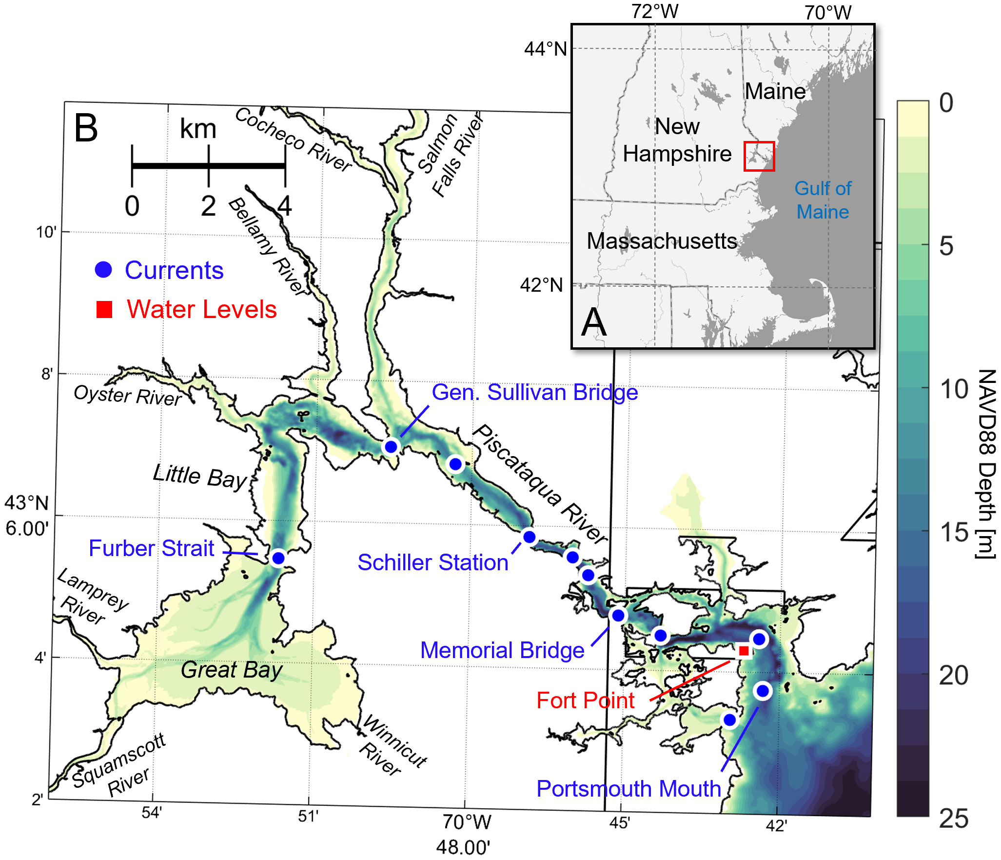
Figure 1 (A) Study region relative to the coast of New England in the United States. (B) Zoom-in of the Piscataqua River – Great Bay estuary with colored contours of bathymetry and locations of current (blue circles) and water level (red square) observations. Rivers and bays in the system are labeled, as well as the main observational locations presented for validation. Vertical datum reference is the North American Vertical Datum 1988 (NAVD88).

The estuary is morphologically complex, with channel depths ranging from relatively deep at the mouth (25 m) to very shallow upstream in Great Bay (~ 3 m). The mouth is relatively narrow (3 km) and constricts further (~300 m) moving into the region between Memorial Bridge and Schiller Station before widening in Little Bay (1 km) and significantly more so in Great Bay (> 5 km) as tidal flat regions increase significantly in size (Figure 1B). Multiple islands and secondary channels exist on both sides of the main channel in the region seaward of the Memorial Bridge, and significant constrictions occur upstream at General Sullivan Bridge (entering Little Bay) and Furber Strait (entering Great Bay). The channelized sections are quite curvy, with frequent bends changing the flow direction by 90 degrees or more (Figure 1B).

Tidal dynamics in the estuary have been studied in the past, and the system follows two main regimes: a highly dissipative region extends from the mouth to Little Bay where the tide behaves like a progressive wave and decays in amplitude and energy moving landward, then a low dissipation region begins near General Sullivan Bridge and moves into Great Bay, where the tide exhibits standing wave qualities and largely maintains its energy (Brown and Trask, 1980; Swift and Brown, 1983; Cook et al., 2019). Former modeling studies of the PRGB system indicate ebb dominance in the lower, Piscataqua River portion of the estuary and flood dominance upstream in Great Bay, with tidally averaged residual flow directed seaward and landward in those regions, respectively (Ip et al., 1998; Ertürk et al., 2002; McLaughlin et al., 2003; Cook et al., 2019).

3 Methods

3.1 Tidal hydrodynamic model

A tidal hydrodynamic model of the PRGB estuary was developed to investigate tidal energy potential and the effect of tidal energy extraction on hydrodynamics. Here, we used the Finite-Volume Community Ocean Model (FVCOM) (Chen et al., 2003) which solves the 3-D Reynold’s averaged Navier-Stokes equations of continuity and momentum with Bousinessq assumptions in hydrostatic mode. FVCOM is a general-purpose ocean model consisting of multiple sub-modules used to simulate numerous physical and biogeochemical processes in the coastal ocean and has been widely applied in modeling tidal energy extraction (e.g., Cowles et al., 2017; Deb et al., in review; Yang et al., 2013; Yang et al., 2014; Li et al., 2017). FVCOM utilizes an unstructured grid modeling framework which is particularly useful for resolving complex estuary and coastline geometries.

Modeling energy extraction via tidal turbines is a requirement of the current study. To achieve this, a current energy converter (CEC) module was implemented in FVCOM which applies the momentum sink approach (Yang et al., 2013; Rao et al., 2016). The method was used in an idealized estuary and validated with analytical solutions (Yang et al., 2013) as well as with flume experiments and a computational fluid dynamics (CFD) model (Li et al., 2017). The CEC module has proven useful in accurately simulating tidal energy extraction and physical-environmental impacts on the surrounding system (e.g., O’Hara Murray and Gallego, 2017; Haverson et al., 2018). In using the CEC module, the governing equations for Reynolds averaged turbulent flows are as follows (Yang et al., 2013):

$\begin{array}{ll}\frac{\partial u}{\partial t}+u\frac{\partial u}{\partial x}+v\frac{\partial u}{\partial y}+w\frac{\partial u}{\partial z}-fv=-\frac{1}{{\rho }_0}\frac{\partial p}{\partial x}+\frac{\partial }{\partial z}\left(K_m\frac{\partial u}{\partial z}\right)+F_x-F_x^M& (1)\end{array}$

$\begin{array}{ll}\frac{\partial v}{\partial t}+u\frac{\partial v}{\partial x}+v\frac{\partial v}{\partial y}+w\frac{\partial v}{\partial z}+fu=-\frac{1}{{\rho }_0}\frac{\partial p}{\partial y}+\frac{\partial }{\partial z}\left(K_m\frac{\partial v}{\partial z}\right)+F_y-F_y^M& (2)\end{array}$

where x, y, and z are the east, north, and vertical coordinates, respectively; u, v, and w are velocities corresponding to the x, y, and z directions; $F_x$ and $F_y$ are the horizontal momentum diffusivity terms in x and y directions; $K_m$ is the vertical eddy viscosity; ${\rho }_0$ is water density; $p$ is pressure; and f is the Coriolis parameter. $F_x^M$ and $F_y^M$ are the additional momentum sink terms associated with energy extraction which are defined as in Yang et al. (2013):

$\begin{array}{ll}\overrightarrow{F^M}=\frac{1}{2}\frac{C_{e}A}{V_c}\left|\overrightarrow{u}\right|\overrightarrow{u}& (3)\end{array}$

where $V_c$ is the momentum control volume where the tidal turbine is located (volume of one 3D grid cell), $A$ is the flow facing area swept by the turbine, $\overrightarrow{u}$ is the velocity vector (u or v), and $C_e$ is the momentum extraction coefficient, which describes the fraction of energy transferred from the water flow to turbines. In this work, $C_e$ is directly prescribed as a constant 0.5 as we are not modeling any specific turbine design, but rather approximating the effect of generic turbines (e.g., Deb et al., in review; Yang et al., 2013). In iterative curve-fitting tests between modelled and observed turbine velocity profiles, Li et al. (2017) found $C_e$ of 0.41 to match observations best, and so a similar value is used here. Further, De Dominicis et al. (2017) tested multiple $C_e$ values on power extraction estimates and concluded that $C_e$ > 0.85 is likely too liberal in energy extraction, and lesser values are most realistic.

3.2 Model grid configuration and boundary conditions

The grid for the PRGB model covers the entire estuary and extends upcoast, downcoast, and offshore of the mouth roughly 15 km. According to International Electrotechnical Commission (IEC) standards, a minimum grid resolution of 500 m is required for a Stage 1 tidal energy feasibility study, and 50 m for a Stage 2 study on layout and design (IEC, 2015). As such, grid resolution within the estuary meets the Stage 2 standard and varies between 15 and 25 m. Moving offshore from the mouth, cell sizes increase to a maximum of 480 m at the open boundary. The unstructured grid was created using the Surface-water Modeling System (SMS) and the variable cell sizes were dictated by bathymetry (higher resolution in regions of higher depth gradients) and a smooth transition between adjacent cells (area transition ratio of 0.7 required). The entire mesh contains ~153,000 nodes and ~293,000 triangular elements, giving exceptional resolution relative to estuary size. Vertical resolution was tested with 20, 10, and 5 terrain-following sigma layers. Results were not meaningfully changed between tests, so 5 uniform layers was applied for run efficiency.

The full mesh bathymetry was created by combining multiple data sets and models. A hierarchal approach was used, where data sets were prioritized first by bathymetry resolution then by recency. Low resolution and/or old data were applied last to fill in any remaining gaps. First, we applied high resolution sonar survey data conducted by the University of New Hampshire (UNH) and the National Oceanic and Atmospheric Administration (NOAA) which extends from the mouth of the Piscataqua River to the entrance of Great Bay (Ward et al., 2021). The NOAA multibeam surveys were taken in 2000 and 2008 and the UNH single beam surveys in 2002. Data from all surveys was gridded at 4 m spacing. The remainder of Great Bay was then covered using a 2015-2016 single beam survey conducted by UNH gridded at 25 m resolution. NOAA navigational soundings (https://www.charts.noaa.gov/InteractiveCatalog/nrnc.shtml) were used in the tidal portions of inflowing tributaries (i.e., Squamscott, Salmon Falls, Cocheco, Bellamy, Lamprey, and Oyster Rivers), in the channels and flats surrounding the islands at the estuary mouth, and in a portion of the grid offshore of the estuary mouth. The soundings had variable resolution less than 1 km. Lastly, the 3 arc-second NOAA Coastal Relief Model (https://www.ncei.noaa.gov/products/coastal-relief-model) was applied to the remainder of the offshore domain not covered by soundings. All vertical datums from the various bathymetry sets were converted to NAVD88 and interpolated onto the model mesh. Wetting and drying of intertidal zones was also explicitly simulated with a minimum depth cut-off criterion of 0.05 m to accurately capture the tidal prism over the extensive mudflat regions in the domain.

The PRGB estuary is dominated by barotropic tidal forcing (Cook et al., 2019). The 10-year mean river discharge to the estuary from the combined tributaries is 49 m³/s, considerably smaller than tidal discharges (Short, 1992; Trowbridge, 2007). Wind-driven mean currents in the PRBG estuary have been found to be enhanced during large storm events but remain of second order importance relative to tidally forced currents (Wengrove et al., 2015). Limited fetch in the system and strong refraction and attenuation of ocean waves at the estuary mouth limit the influence of waves on water velocities and sea surface heights (Cook et al., 2019). Further, the estuary is well-mixed and so buoyancy driven flows are considered negligible (Cook et al., 2019). As such, river, wind, wave, and buoyancy (salinity, temperature) forcing are omitted from this study. These omissions also allow us to identify modulation to strictly barotropic tide forced dynamics in the system more easily. The tidal open boundary condition was specified with elevation time series obtained from the Oregon State University (OSU) TPXO global ocean tide database (Egbert and Erofeeva, 2002) and included 13 tidal constituents: M₂, S₂, N₂, K₂, K₁, O₁, P₁, Q₁, M₄, MS₄, MN₄, M_m, and M_f.

The model was initialized with zero velocity and free surface elevation throughout the domain. A 5-day spin-up period was omitted from analysis to allow the model to reach dynamic equilibrium. Simulations were performed for one 3-month period from May 1 to July 31, 2007, which allowed a minimum 35-day model-data comparison for all tidal current observations conducted by NOAA in the estuary (see Table 1). The same period was used for tidal hydrodynamics analysis. Model results were output at 15-minute intervals at every mesh node and cell. Bottom friction follows the quadratic law with the drag coefficient determined by the logarithmic bottom layer as a function of bottom roughness. The bottom drag coefficient and roughness height were specified as C_d = 0.0025 and Z₀ = 0.02m, respectively. Multiple roughness heights were tested for the same simulation period, with 0.02 m providing the best error statistics, similar to the findings of Cook et al. (2019) and Swift and Brown (1983).

TABLE 1

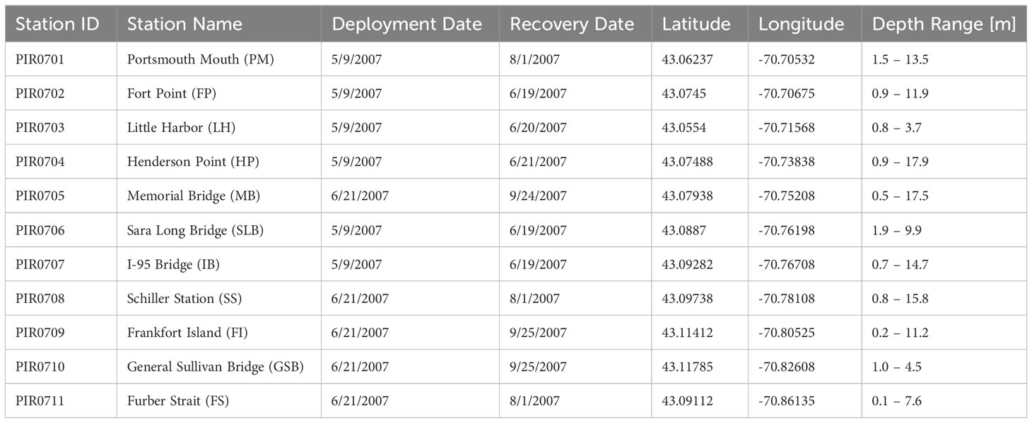
Table 1 Depth-varying current (ADCP) sampling locations, deployment durations, positions, and sampling depths in the Piscataqua River – Great Bay estuary.

3.3 Observational data

In total, 11 acoustic Doppler current profiler (ADCP) stations measuring depth-varying currents and 1 tide gauge measuring water level elevation were used for model validation (see Figure 1). Additional tidal predictions at 7 XTide stations throughout the estuary were used to check the limited water level observations (not shown). The tide gauge, maintained by NOAA, was located at Fort Point, NH near the mouth of the estuary (station #8423898). The gauge was decommissioned in 2020, but historical data is still available at: https://tidesandcurrents.noaa.gov/stationhome.html?id=8423898.

Current data was also collected by NOAA through the Currents Measurement for the Study of Tides (CMIST) program. NOAA deployed the 11 upward looking, bottom mounted ADCPs on either 05/09 or 06/21/2007 and retrieved them on multiple days between 6/20 and 9/25/2007 (Table 1). The sensors used in this campaign were both 600 and 1200 kHz Teledyne Workhorse ADCPs and all sampled at 6 min. intervals. Each ADCP sampled in 1 m vertical bins, except locations LH, GSB, and FS which were 0.5 m (Table 1). Blanking distances above each sensor were 0.88 m and 0.44 m for those sampling every 1 m and 0.5 m, respectively, while all sensor platforms were 0.85 m from the bottom. Depth ranges sampled in the deployment varied between 3 m and 17 m, depending on location (Table 1).

3.4 Model validation

3.4.1 Water levels

The model performance in simulating tidal water levels was evaluated by comparing the observed data at the Fort Point tide gauge to model results at the same location over a 15-d. period from 6/23 to 07/08/2007 (Figure 2A). The simulated water levels match observations quite well, and accurately depict spring-neap variability as well as the minor diurnal inequality. Comparison to the supplemental XTide water level predictions upstream were also favorable and captured spatial variability in tidal amplitude and phase (not shown).

FIGURE 2

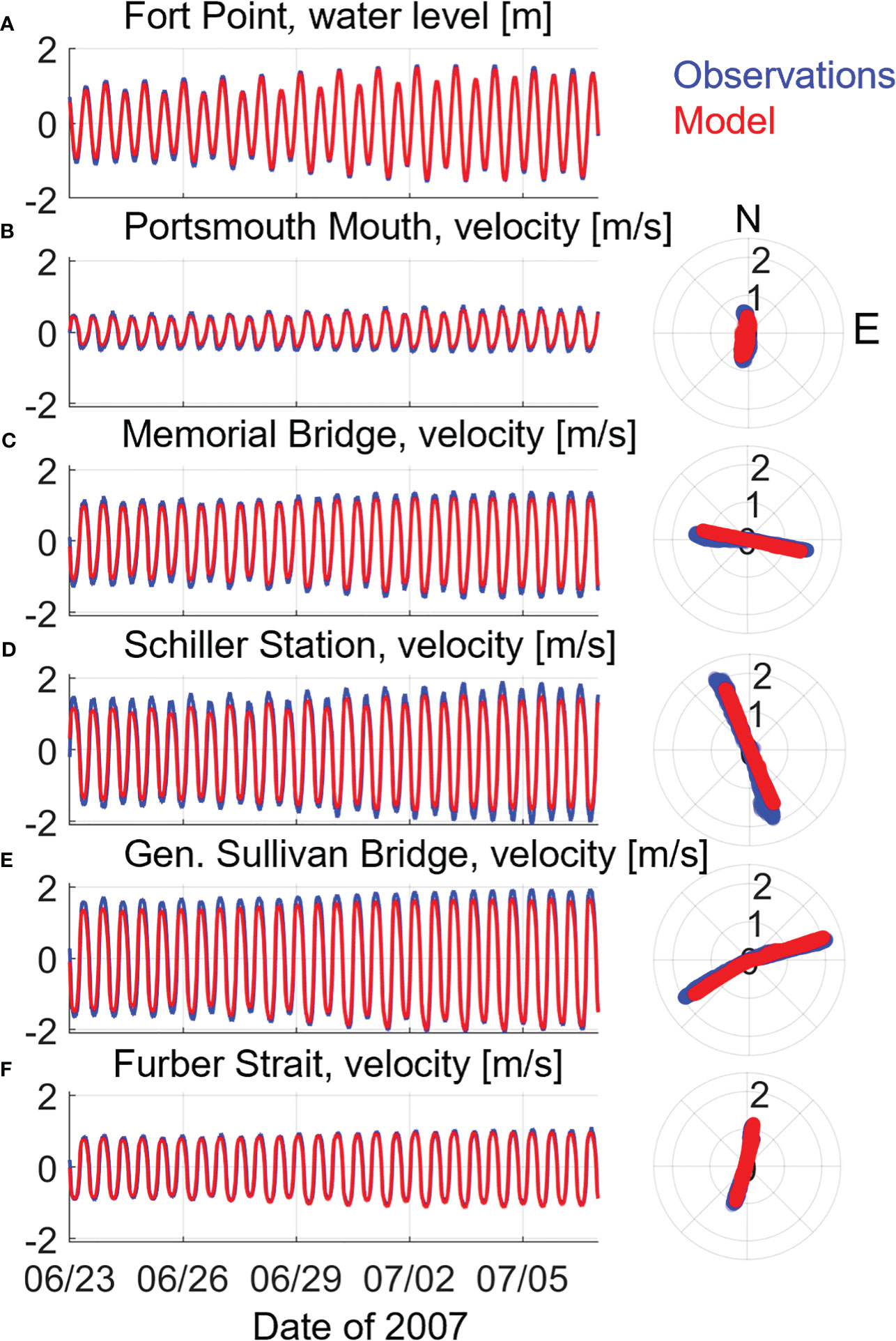
Figure 2 Time series of modeled (red) versus observed (blue) Fort Point water levels (A) and depth-averaged principal component current velocities (B–F). Velocity time series (left) are accompanied by scatter plots comparing velocity magnitude and direction in compass bearings (right) at the Portsmouth Mouth (B), Memorial Bridge (C), Schiller Station (D), General Sullivan Bridge (E), and Furber Strait (F) ADCP stations.

Four error statistical parameters were used to quantify the model skill in reproducing water levels. The statistics were calculated over the entire 3-month model simulation period. The root-mean-square-error (RMSE):

$\begin{array}{ll}RMSE=\sqrt{\frac{{\sum }_{i=1}^N{(P_i-M_i)}^2}{N}}& (4)\end{array}$

where N is the total number of observations and modeled points, M_i is the measured value, and P_i is the modeled (predicted) value. The scatter index (SI) is the RMSE normalized by the average magnitude of measurements, $\overline{\left|M\right|}$:

$\begin{array}{ll}SI=\frac{RMSE}{\overline{\left|M\right|}}& (5)\end{array}$

The bias is the mean difference between observations and model predictions:

$\begin{array}{ll}Bias=\frac{{\sum }_{i=1}^N(P_i-M_i)}{N}& (6)\end{array}$

Lastly, the linear correlation coefficient (R) measures the linear relationship between model predictions and observations:

$\begin{array}{ll}R=\frac{{\sum }_{i=1}^N(P_i-\overline{P})(M_i-\overline{M})}{\sqrt{\left({\sum }_{i=1}^N{(M_i-\overline{M})}^2\right)\left({\sum }_{i=1}^N{(P_i-\overline{P})}^2\right)}}& (7)\end{array}$

The RMSE for water levels at Fort Point is 0.12 m, which is quite satisfactory given the large tidal amplitude at the Piscataqua River mouth. The normalized SI is 0.14, the bias is -0.07 m, and the correlation coefficient, R, is 0.995, all of which are very favorable values for model-observation comparison.

In addition to error statistics, the amplitudes and phases of the dominant semidiurnal (M₂) and diurnal (K₁) tides as well as the two most significant overtides in the estuary (M₄, M₆) were calculated for both the observations and model output at Fort Point and compared in Table 2. Amplitudes and phase values, with 95% confidence interval error estimates, were calculated via harmonic analysis using the UTide MATLAB toolbox (Codiga, 2011). Modeled and observed values generally compare quite well and fall within or very close to the error bounds of each other for all harmonics, indicating tidal constituents are sufficiently simulated in water levels. Harmonic analysis also illustrates the dominance of the M₄ over M₆ overtides in this portion of the estuary, consistent with previous work (Cook et al., 2019).

TABLE 2

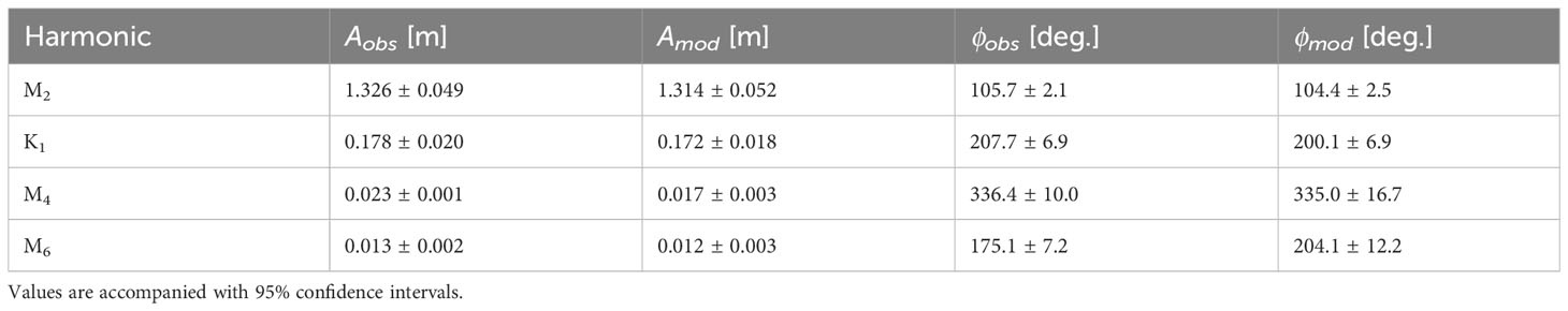
Table 2 Comparison of observed (obs) and modeled (mod) tidal constituent amplitudes (A) and phase lags (ϕ) for water levels at the Fort Point tide gauge for the M₂, K₁, M₄, and M₆ harmonics.

3.4.2 Currents

A similar series of tests between model and observations was performed to evaluate model skill in simulating tidal currents. Figures 2B–F gives 15-d. time series model-data comparisons of depth-averaged, principal axis currents at 5 ADCP locations throughout the estuary, as well as current direction. Depth averaging for both ADCP data and model output was only over the depth range sampled by the ADCP at a particular location. Modeled current magnitudes and directions match the data well, with the only deviations being a slight underprediction of maximum current magnitudes at the locations with the largest velocities (i.e, Memorial Bridge, Schiller Station, Figures 2C, D). The time series’ also show the dominating influence of the semidiurnal (M2) tide in currents, the amplification of current magnitudes within the narrow, channelized Piscataqua River section (Memorial Bridge to General Sullivan Bridge), and the upstream weakening of currents through Furber Strait into the Great Bay (Figure 2).

Error statistics (Equations 4 – 7) were calculated for the depth-averaged, principal component velocity at all ADCP locations (Table 3). The maximum RMSE is 0.23 m/s which is acceptable relative to the maximum current magnitudes at that station (Schiller Station) approaching 2 m/s. Excluding Little Harbor, SI maximizes at 0.37, bias is less than 0.07, and R greater than 0.985. The Little Harbor location is located just south of Portsmouth Mouth (see Figure 1) between two jetties entering a shallow side channel. Slightly elevated SI (0.4), bias (-0.14 m/s), and decreased R (0.973) relative to other locations is likely due to the complicated, shallow bathymetry and geometry in that area which may be lacking features in the model due to lower resolution depth soundings applied there. Either way, error statistics in the remaining, main channel locations are very favorable.

TABLE 3

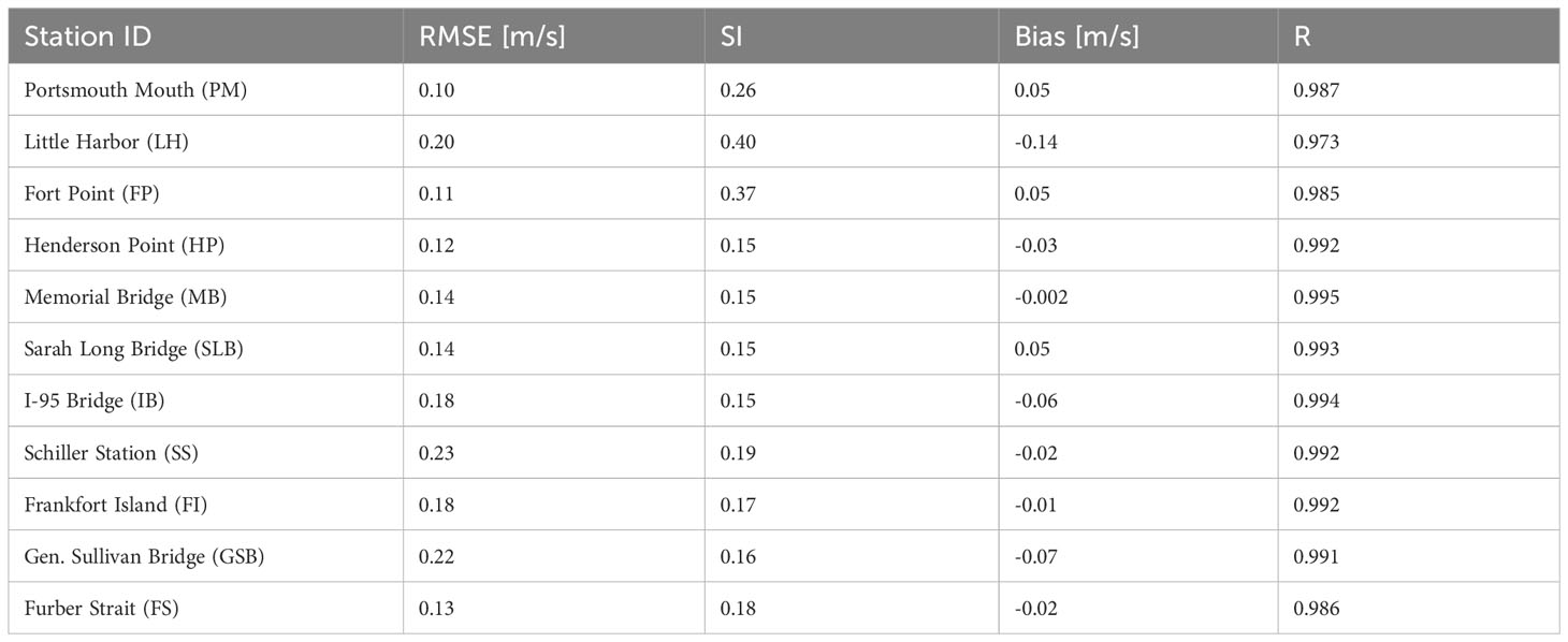
Table 3 Model – observation error statistics for depth-averaged, principal axis currents at all ADCP stations in the Piscataqua River – Great Bay estuary.

The amplitudes and phases of the M₂, K₁, M₄, and M₆ harmonics were also calculated for the depth-averaged, principal component velocities at each ADCP station (Figure 3). M₂ and K₁ amplitudes match well, while phase comparisons are nearly identical (Figures 3A–D). Similarly, modeled and observed M₄ and M₆ overtide signals compare favorably. The largest relative differences occur in the M₄ amplitude (25-50%) but only at a few locations (i.e, Frankfort Island [FI] and I-95 Bridge [IB], Figure 3E). Regardless, the generally spatial trends in M₄ amplitude are similar, as are the phases (Figure 3F). Previous modeling studies in the PRGB estuary found the largest data-model discrepancies in the M₄ signal as well (Cook et al., 2019). It is possible there are local, internal asymmetries due to time variations in turbulent stresses and shear within the water column contributing to these differences (e.g., Jay and Musiak, 1996; Ross et al., 2017) or modification to flow asymmetry from nearby headlands and estuary curvature (Lieberthal et al., 2019). Both mechanisms contribute to M₄ current signals but are hyperlocal in their effects, so small spatial discrepancies between modeled and observed flow fields or mixing could give differing results.

FIGURE 3

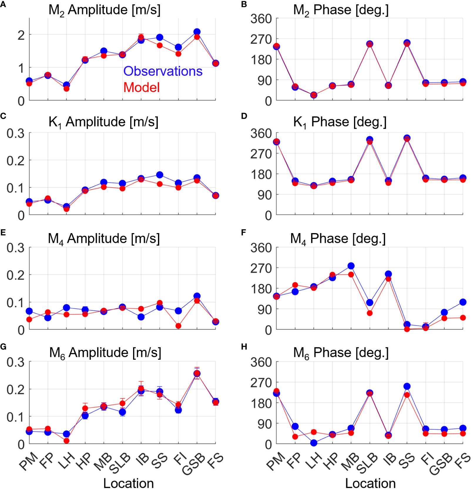
Figure 3 Modeled (red) and observed (blue) M₂ (A, B), K₁ (C, D), M₄ (E, F), and M₆ (G, H) amplitudes (A, C, E, G) and phases (B, D, F, H) for depth averaged principal axis currents at all ADCP stations. Error bars denote 95% confidence intervals.

3.5 Tidal turbine farm siting and design

With the model skill validated, we next designed a tidal energy extraction simulation to investigate the effect of energy extraction on hydrodynamics in the PRGB estuary. A hypothetical tidal turbine farm was placed in the system using realistic siting parameters. Ideally, tidal turbine arrays should be placed in regions of significant power extraction potential in water deep enough to allow maritime navigation. Power potential in the estuary was evaluated by calculating the power density, P (W m^-2), over the full domain:

$\begin{array}{ll}P=0.5{\rho }_w{\overline{V}}^3& (8)\end{array}$

where $\overline{V}$ is the depth-averaged current speed. One year-long (all of 2007) simulation of the validated PRGB model was run with no turbines and Equation 8 was calculated at each grid cell at each time step then time averaged. Figure 4A shows the annual mean power density over the lower and middle reaches of the Piscataqua River where the magnitudes appeared. Significant tidal power density (> 1 kW m^-2) was identified in two regions: around General Sullivan Bridge and between Fort Point and Schiller Station (Figure 4A), all located in the more channelized, constricted portions of the Piscataqua River where tidal currents are largest (Figure 2).

FIGURE 4

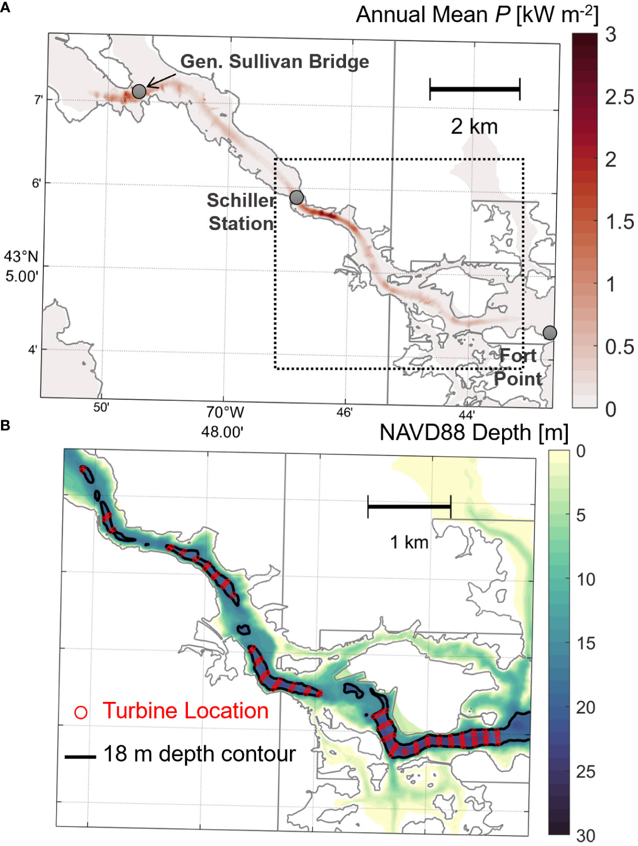
Figure 4 (A) Planview map of annual mean power density, P, over the most energetic portion of the Piscataqua River. Colored contours represent P. Three reference locations are marked with gray circles and labeled. (B) Zoom-in on the dotted line box from (A), showing the simulated tidal turbine configuration. Depth is given as a colored contour with the 18 m isobath denoted as a solid black line. Turbine cell locations are colored with red circles. In total, 180 turbines are marked.

We next evaluated depths in the two high energy regions. Maximum depths in both regions are greater than 18 m in the center channel (Figure 1). Generally, the section nearer the mouth features larger swaths of >18 m depths, uniform across the entire channel, more favorable for multiple rows of multiple turbines. As such, we chose this region (Fort Point to Schiller Station) as the best site for a potential tidal turbine farm (Figure 4B). The region around General Sullivan bridge remains favorable for tidal energy extraction, but the shallower depths would limit turbine diameter further. In this study, we chose to limit our energy extraction scenario to the deeper region near the mouth. Future investigations will explore the differing influence of turbine array location on dynamics.

Turbine dimensions were specified based on channel depths and navigation requirements. The average ship which navigates the river to access Portsmouth Harbor requires a draft of 8 m (U.S.A.C.E., 2014), which can be considered the minimum clearance needed between a turbine and the water surface. Using 18 m as a minimum depth requirement and 8 m as a minimum clearance, a 10 m diameter turbine with a center hub 5 m above bottom was considered acceptable for this farm design, with past studies using similar dimensions (Yang et al., 2014).

The modeled turbines were placed in rows bounded by the 18 m depth contour on either end. Rows were spaced 15 rotor-diameter spaces apart (150 m) to minimize downstream wake effects while individual turbines in each row were spaced 2 rotor-diameters apart (20 m) to similarly allow lateral wake dissipation. Channel sections which shallowed to less than 18 m or did not allow a minimum of 3 turbines per row were kept open (Figure 5). The total array was comprised of 180 turbines, which would be considered a relatively large-scale but realistic tidal energy farm (see below). One 2-month simulation covering part of the model validation period (June, July 2007) was run with the full turbine array allowing analysis of hydrodynamic impacts within the estuary.

FIGURE 5

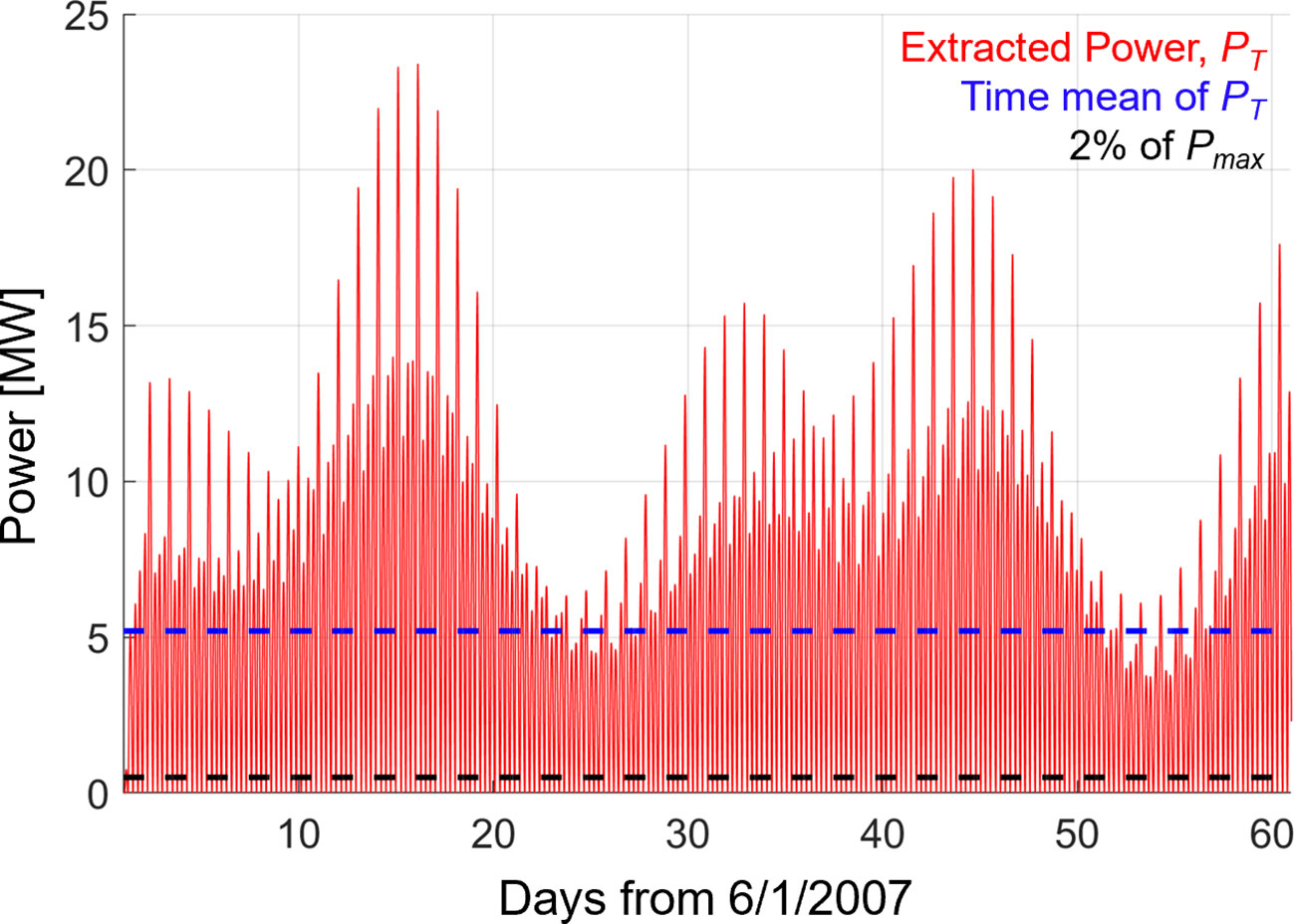
Figure 5 Time series of turbine extracted power, P_T, in the PRGB estuary during a 2-month simulation in 2007 (red). The temporal average of P_T and 2% of P_max are shown as the dashed blue and black lines, respectively.

We estimated the amount of power our hypothetical turbine array is capable of extracting, so this configuration can be placed in the context of others and the theoretical power potential of the PRGB estuary itself. The maximum time averaged power which can be extracted from the system, $P_{max}$, was determined using the analytical expression of Garrett and Cummins (2005) and was quantified at a section crossing the mouth of the PRGB estuary:

$\begin{array}{ll}{P}_{max}=\gamma {\rho }_wɡa_0{Q}_{max}\left[1+\frac{9}{16}\left({\sum }_{i=1}^{Mt}{\left(\frac{a_i}{a_0}\right)}^2\right)\right]& (9)\end{array}$

where $\gamma$ is a time-dependence coefficient (0.22), g is the gravitational acceleration, $a_0$ is the largest tidal constituent amplitude at the section (M₂), $Q_{max}$ is the maximum tidal discharge through the section, and $a_i$ are the additional $M_t$ tidal constituent amplitudes (i = 1, 2, … $M_t$). The full year base simulation was used to find $Q_{max}$ and tidal constituent amplitudes, which were determined using UTide. Using (9), $P_{max}$ is estimated to be ~24 MW.

Next, the time varying power extracted by each turbine, $P_T$, was calculated similar to Deb et al. (in review) and De Dominicis et al. (2017):

$\begin{array}{ll}{P}_T=0.5{\rho }_w{C}_p{A}_b{V}^3& (10)\end{array}$

where $C_p$ is the turbine power coefficient, and V is the average current speed through the turbine. $C_p=1$ here, which assumes all the kinetic energy from the flow is converted to power. Efficiency losses are likely in reality, but the exact amount is unknown. The summed power provided by all 180 turbines over June and July 2007 is given in Figure 5 to illustrate temporal variability in extracted power, which varies from ~6.6 MW maxima during neap tides to nearly the theoretical maximum, $P_{max}$ (~23 MW), during spring tides. The full simulation mean (2 months for the turbine run) of $P_T$ equals ~5.1 MW (shown in Figure 5), roughly 20% of $P_{max}$. According to IEC (2015) standards, an annual average extracted power greater than 2% of $P_{max}$ (~0.5 MW, shown in Figure 5) is considered a large tidal turbine project in the system and the effect of energy extraction should be simulated dynamically. Although the average power calculated does not cover a full year, we expect the annual and 2-month means are similar given the periodic nature of tides, and consider this turbine array a large project. The expected annual power production (AEP, in kWh) can then be estimated by multiplying the average power extracted by the turbines (5.1 MW) by the number of hours in a year (8760 hr.), giving 44.7 GWh.

4 Results

4.1 Currents: spatial variability and turbine effects

First, we evaluated how the tidal turbine array modifies the spatial (horizontal and vertical) variability in depth-averaged currents throughout the PRGB estuary. Histograms of depth-averaged current speeds were created at four ADCP locations moving from the mouth (Fort Point) to inland (Furber Strait) to identify changes to current magnitude probability density distributions (PDFs) in an energy extraction scenario (Figure 6). At Fort Point, near the mouth, the base case speeds generally follow a normal distribution peaking around ~0.5 m/s (Figure 6A). For the remaining inland locations, speeds are log-normal with skew towards the faster end of the spectrum, typically peaking between 1 and 1.5 m/s (Figures 6B–D). When turbines are added, all distributions lose currents at the highest speeds and shift toward the slower side of the spectrum to varying degrees, suggesting a net reduction in current speeds at these channel locations. At the middle Piscataqua River sections (Memorial Bridge and General Sullivan Bridge), the locations with the fastest currents, the most notable changes are seen with peaks shifting to currents 0.3 – 0.5 m/s slower than the base case (Figures 6B, C). Changes are less extreme at the mouth (Fort Point) and entering Great Bay (Furber Strait), but the fastest currents are still slowed the most at those locations as well (Figures 6A, D).

FIGURE 6

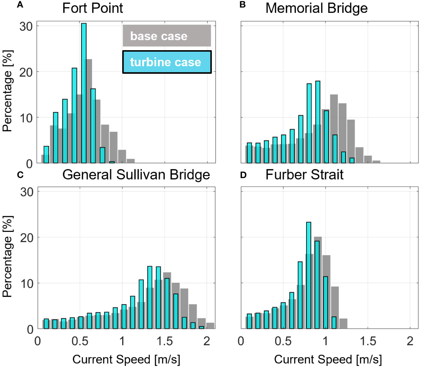
Figure 6 Histogram of depth-averaged current speed distributions at the Fort Point (A), Memorial Bridge (B), General Sullivan Bridge (C), and Furber Strait (D) locations for the base (gray) and turbines included (cyan) simulations. X-axis is binned current speeds and y-axis is the percentage of total data points in each bin.

To better grasp spatial variability in current modulation and isolate where turbine effects are most significant, time and depth-averaged currents over a spring-neap cycle (15 d.) were compared over the entire model domain. Further, 15-day averages in currents can be considered a metric for residual flows in the estuary and indicate how tide-averaged transport behaves and could be modified under energy extraction. In the base simulation, residual current magnitudes are strongest (0.3 – 0.5 m/s) in the vicinity of major channel bends and headlands (i.e., Fort Point and General Sullivan Bridge regions, Figure 7A). In these areas, residual currents are generally strongest over the shoals with opposing directions over each shoal, indicative of differential advective accelerations driven by cross-channel variability in maximum flood and ebb currents (e.g., Ross et al., 2021). Away from these regions, residual currents are of order ~0.1 m/s, landward directed in the center channel of Great Bay, and seaward directed over the remainder of the main Piscataqua River channel (Figure 7A), matching past work in the estuary (Ip et al., 1998; McLaughlin et al., 2003). When turbines are included, the main affect is a general reduction in residual currents systemwide (up to 0.1 m/s), but most notably in the lower Piscataqua River between the mouth and the Schiller Station constriction (Figure 7B). In that region, residual currents are locally increased over channel edges and shoals in and around the tidal turbine farm by up to 0.1 m/s (Figure 7B), a typical effect of flow bypassing turbines in the center channel (e.g., Wang and Yang, 2017).

FIGURE 7

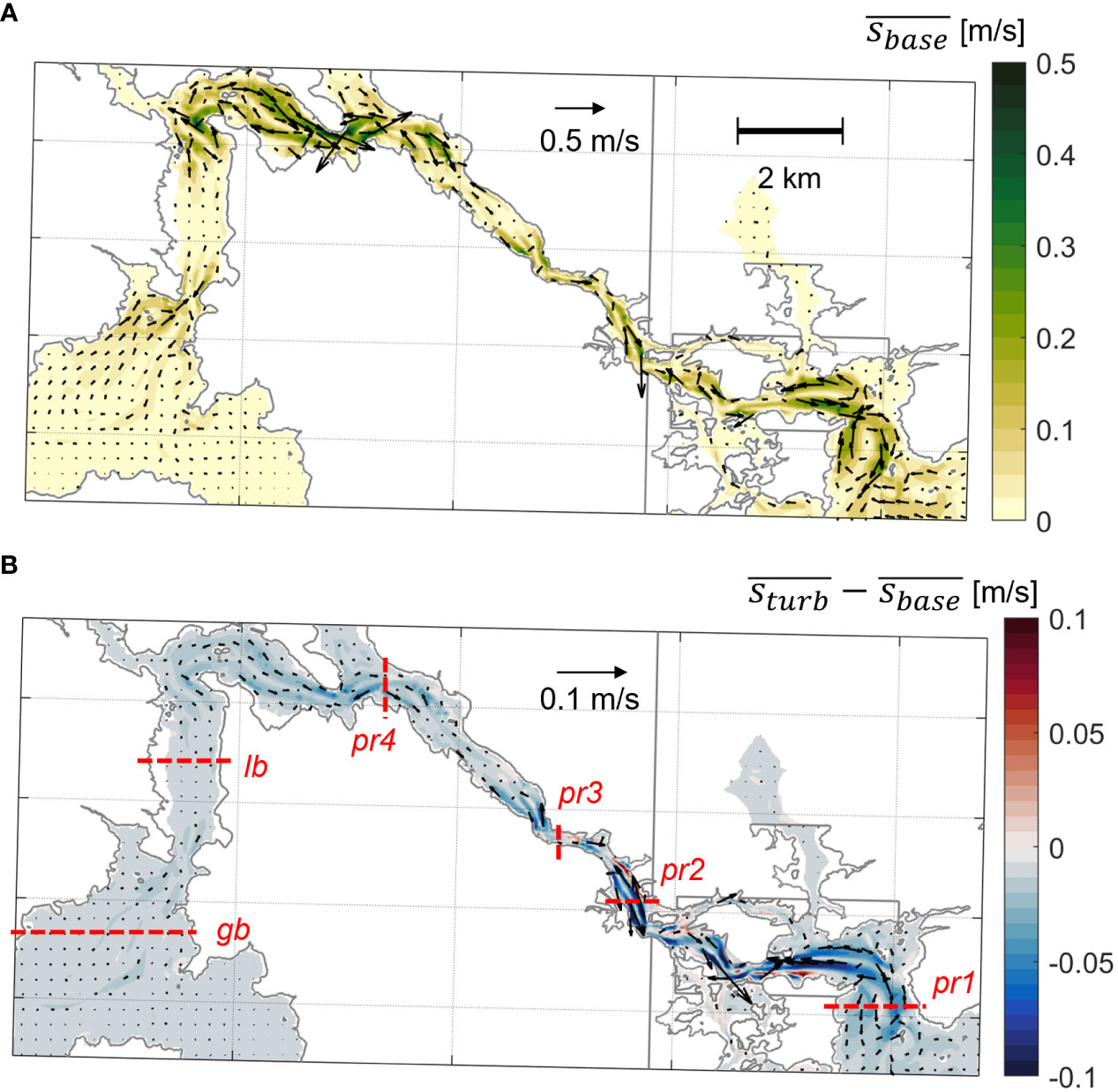
Figure 7 Planviews of (A) 15 day depth-averaged residual current speed (s, colored contour) and direction (arrows) for the base simulation and (B) difference in depth-averaged residual current speeds (colored contour) and direction (arrows) between the turbine and base runs. Warm colors in (B) indicate faster currents in the turbine simulation, cold colors indicate slower. Red dashed lines indicate the cross sections used in forthcoming analysis and are labeled. Currents were linearly interpolated onto a uniform grid from the unstructured mesh and vectors are provided at every 8^th grid point.

Vertical variation to current structure in the lower Piscataqua River region was illustrated with flood and ebb tidal phase comparisons of principal axis currents at section pr2 during a “typical” tide in the middle of a spring-neap cycle (Figure 8, see Figure 7B for pr2 location). In the base simulation, flood (ebb) tides feature predominately seaward (landward) directed flow in the main channel with maximum current magnitudes (~1.5 m/s) between surface and mid water column, reductions in current magnitude moving laterally away from the maximum location to channel sides, and flow over the shallow eastern shoal (0 – 200 m on x-axis) opposing the direction of channel currents (Figures 8A, D), likely from recirculation around the islands north/east of the channel (see Figure 7). The section presented also nicely shows why residual flow magnitudes and direction may be so variable across select channel sections (Figure 7): although both flood and ebb tides feature similar magnitude current maxima, the locations of those maxima do not occur at the same lateral location in the channel (Figures 8A, D). The strongest flood tide currents hug the western side of the channel (Figure 8A, 500 – 600 m on x-axis) while during ebb the maxima occur over the eastern side and channel center (Figure 8D, 250 – 500 m on x-axis). Time averages of this successive lateral asymmetry leads to relatively strong residual flows biased to one tidal phase (landward or seaward) over the other on opposite sides of the channel and can be attributed to frequent changes in curvature throughout the estuary. During the turbine simulation, the cross-channel structure of principal axis currents is largely like the base case: maximum currents occur in the same channel locations, decrease towards channel edges, and feature opposing flow on the eastern shoal (Figures 8B, E). The major effect of the turbines is a notable reduction in the maximum current magnitudes by 0.3 – 0.4 m/s and a more modest increase in currents on the channel sides (0.1 – 0.2 m/s), during both flood and ebb tides (Figures 8C, F). This further illustrates the flow bypass effect of turbines: the fastest currents over the deepest channel sections are slowed because turbines (momentum sinks) are placed there. Some of the principal flow therefore diverts to the channel sides/shoals, increasing current magnitudes there, but to a smaller degree than the reduction in currents mid-channel.

FIGURE 8

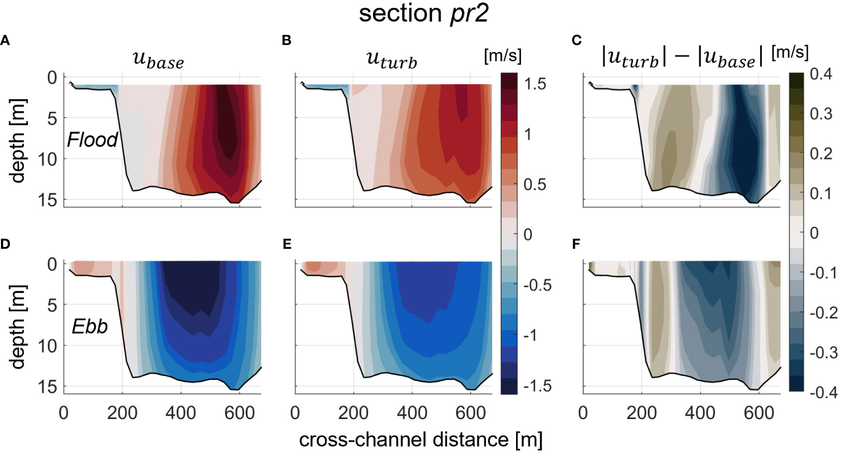
Figure 8 Cross-channel (x-axis) and depth varying (y-axis) principal axis velocity snapshots during maximum flood (A, B) and ebb (D, E) currents at section pr2 (see Figure 7) during a typical tide on 6/20/2007. The base simulation is shown on the left (A, D), the turbine run in the middle (B, E), and the difference in current magnitudes is on the right (C, F). Warm colors in (A, B, D, E) indicate landward directed currents and cold are seaward. Perspective is seaward facing.

4.2 Tidal transport and asymmetry

We have shown that a hypothetical tidal turbine farm acts to reduce currents, both residual and tidal, throughout the PRGB estuary domain, with spatially small, localized exceptions. The fastest currents in the main channel are reduced the most, and this effect is most notable in the lower Piscataqua River reach between the mouth and Schiller Station. It remains unclear how the turbines modulate tidal (flood/ebb) transport and asymmetry along the estuary. Prior to further analysis on the topic, it is pertinent to provide more background on how barotropic tides can become distorted in shallow, well-mixed estuaries.

Former work has established that in relatively shallow, well-mixed estuaries where $a/h$ (tidal amplitude/water depth) is large, tidal asymmetry can be created by the shallow water effect, bottom friction, and/or estuary geometry (Friedrichs and Aubrey, 1988; Parker, 1991). Assuming friction is negligible, the shallow water effect causes the crest of the tidal wave to travel faster than the trough, resulting in shorter, faster flood tides and longer, slower ebbs (flood dominance) (Dronkers, 1986; Friedrichs and Aubrey, 1988). In reality, friction must also be considered in short estuaries as tidal propagation is otherwise complicated by co-oscillation due to reflection. Friction acts to exaggerate flood dominance as more frictional momentum is lost during low water than high (Uncles, 1981; Dronkers, 1986). The combined shallow water and friction effects (represented as depth-dependent quadratic friction in the equations of motion and referred to as such from here on) thus create water level changes are slower around low tide within the estuary than at the mouth, and a larger time lag between mouth and upstream low waters exists relative to high waters, giving longer, weaker ebbs and shorter, faster floods. If an estuary features large intertidal zones (wetting and drying flats) relative to deep channels, tidal asymmetry may shift to ebb dominance (Boon and Byrne, 1981; Speer and Aubrey, 1985; Friedrichs and Aubrey, 1988). During low water, intertidal flats are empty while deep channels remain submerged, giving a relatively quick transition to flood. At high water, the shallow flats are submerged and the transition to ebb is slowed, with the net result being shorter, faster ebbs than floods. Some estuaries may feature both flood and ebb dominant regimes dependent on along-channel variation in each mechanism (e.g., Brown and Davies, 2010). (Friedrichs and Aubrey, 1988).

Friction can further modulate the barotropic tide in a symmetric manner. At first order, friction decreases the tidal wave celerity and dampens the wave amplitude. This linear mechanism does not distort the tidal wave, but rather equally delays the timing and decreases the magnitude of high and low water levels (Parker, 1991). Conversely, nonlinear quadratic friction distorts the wave, but unlike depth-dependent friction described previously, only relies on tidal current magnitude. As such, maximum quadratic friction momentum loss and minimum wave celerity occur during both maximum flood and ebb currents, while slack waters feature the opposite, leading to fluctuations in currents and sea surface over a tidal cycle scaling with current magnitude (Parker, 1984; Parker, 1991).

With a background on tidal distortions in transport and water level established, we next calculate cross-sectionally averaged, section normal velocities and volume fluxes at six cross sections in each sub-region of the PRGB estuary: the Piscataqua River: pr1, pr2, pr3, and pr4; Little Bay: lb; and Great Bay: gb. Here, volume flux, Q, is a proxy for transport and is calculated by integrating the section normal velocity, $u_n$, across-channel and with depth:

$\begin{array}{ll}Q=\iint u_{n}dx dz& (11)\end{array}$

The maximum flood and ebb volume fluxes, $Q_f$ and $Q_e$, respectively, as well as velocities, $u_{n,f}$ and $u_{n,e}$, are presented for the same tidal cycle shown in Figure 8 to identify spatial variability in velocity and transport, the impact of turbines on transport in and out of the PRBG estuary, and to qualitatively show tidal asymmetry regimes (i.e., flood or ebb dominance) and sensitivity to turbines (Figure 9). Expectedly, flood and ebb volume fluxes both decay in magnitude moving from the estuary mouth to head, while currents are strongest in the narrow channels of the Piscataqua River. More pertinent to this work are the notable inequalities between flood and ebb transports and currents at the stations nearest the mouth (pr1, pr2, pr3, Figures 9A, B). In the base case, $Q_f$ = 5500 m³ s^-1 at pr1, while $Q_e$ is larger in magnitude by 700 m³ s^-1 at the same location ($Q_e$ = 6200 m³ s^-1, Figure 9A), indicative of ebb dominant tidal asymmetry. $Q_e$ dominance over $Q_f$ decreases moving landward, both transports appear nearly equal at pr4, then dominance swaps in the upstream bays as $Q_f$ slightly exceeds $Q_e$ on the order of 100 m³ s^-1 (lb, gb, Figure 9A), showing a transition from ebb dominance to flood dominance. Section averaged velocities largely follow suit: ebb current magnitudes dominate over flood from pr1 to pr4 by up to 0.1 m s^-1, then appear nearly equal at lb and gb (Figure 9B). When turbines are simulated, both flooding and ebbing transports and currents decrease in magnitude at all sections, but larger reductions occur for ebb relative to flood, and the largest decreases in ebb transport and velocity occur in the Piscataqua River sections of the estuary. At the mouth (pr1), turbines act to reduce flood transport by 450 m³ s^-1 and currents by 0.02 m s^-1, while ebb transport is decreased by a larger factor of 620 m³ s^-1 and currents by 0.03 m s^-1(Figures 9C, D). The Piscataqua River sections (pr1, pr2, pr3, and p4) on average see decreases in ebb transport and currents larger in magnitude than reductions to flood: ~120 m³ s^-1 and ~0.03 m s^-1 larger for transport and currents, respectively (Figures 9C, D). Greater reductions to ebb transport relative to flood in regions of ebb dominance signal tidal asymmetry is likely being diminished. The more equal reductions in flood and ebb transport in the flood dominant, upstream sections (lb, gb, Figure 9B) imply likely little change to tidal asymmetry there, and spatial variability exists in how asymmetric tidal distortion is modulated by turbines.

FIGURE 9

Figure 9 Along estuary (x-axis) variability in max flood (solid line) and ebb (dashed line) volume fluxes, Q (A), and cross-sectionally averaged, section normal velocity, u_n (B), for base (black) and turbine (gray) simulations for the same tidal cycle presented in Figure 8. The difference in magnitude in max volume fluxes (C) and velocity (D) between the turbine and base simulation for both flood (solid) and ebb (dashed) tides. Sections are labeled in (A).

We may quantitatively characterize the magnitude of tidal distortions and asymmetry initiated by the aforementioned nonlinear mechanisms via amplitude and phase relations between the principal, astronomical tide and higher frequency constituents directly resulting from nonlinear interactions (Friedrichs and Aubrey, 1988) which we call overtides or compound tides (Godin, 1986). In an estuary forced by the semidiurnal M₂ tide, the M₄ (fourth diurnal) overtide grows with the asymmetric mechanisms (shallow water, depth-dependent friction, estuary geometry). As such, the amplitude ratio of $A_{M4}/A_{M2}$ scales with the magnitude of tidal asymmetry whereas the phase ($\theta$) relation, $2{\theta }_{M2}-{\theta }_{M4}$, indicates either flood (0 – 180 degrees) or ebb (180 – 360 degrees) dominance (Friedrichs and Aubrey, 1988). Another major overtide, the M₆, indicates the effect of non-depth dependent quadratic friction (i.e., tidal current only) on the tide, and the amplitude ratio $A_{M6}/A_{M2}$ scales with quadratic frictional distortion (Parker, 1984). Like principal tidal harmonics, overtide signals are present in both sea surface heights and current velocities.

Amplitudes and phases of the primary M₂ tide and the major overtides: M₄ and M₆ were calculated to quantify along-estuary variability in distortions and the effect of tidal energy extraction to confirm the trends outlined in Figure 9. Full (2 month) time series of water levels at each section were used to calculate amplitudes and phases with UTide. First order changes to water levels are reflected in the generally decreased M₂ tidal amplitude landward of the turbine array (pr2 thru gb, Figure 10A). $A_{M2}$ dampens an average of 10 cm between pr2 and gb (Figure 10A), translating to a modest tidal range reduction of 20 cm. Similar decreases in $A_{M4}$ and little change to $A_{M6}$ relative to $A_{M2}$ with the addition of turbines (Figures 10B, C) suggests that the damped astronomical tide is not transferring more energy to higher order harmonics via stronger nonlinear mechanisms, but rather is experiencing stronger linear frictional effects acting to attenuate the wave profile (Parker, 1991). Thus, we may note that an important impact of tidal turbines here is to effectively increase the linear frictional decay of the tidal wave as is propagates landward. Additionally, $\raisebox{1ex}{$A_{M4}$}\!\left/ \!\raisebox{-1ex}{$A_{M2}$}\right.$, which quantifies the strength of asymmetric tidal distortion, is also reduced anywhere from 5% upstream at Little Bay to 70% approaching the mouth at pr2 (Figure 10B). The larger reduction in asymmetry in the Piscataqua River sections relative to Little Bay and Great Bay confirm the trends outlined in flood and ebb transport patterns presented previously (Figure 9). The phase relation between M₂ and M₄ tides: $2{\theta }_{{\eta }_{M2}}-{\theta }_{{\eta }_{M4}}$, where ${\theta }_{{\eta }_{M2}}$ is the Greenwich phase of M₂ water levels and ${\theta }_{{\eta }_{M4}}$ is the same for M₄, also confirms our claim that the PRGB estuary is ebb dominant seaward of Little Bay (and intertidal storage is likely important to asymmetry), nearly symmetrical in Little Bay, and flood dominant in Great Bay (where shallow water/friction is likely important to asymmetry) (Figure 10D). Notably, the addition of the tidal turbine farm does not change any region from flood to ebb dominant or vice versa: it appears the turbines mainly reduce the magnitude of ebb dominant asymmetry in the Piscataqua River sections and negligibly modify asymmetry in the upstream bays.

FIGURE 10

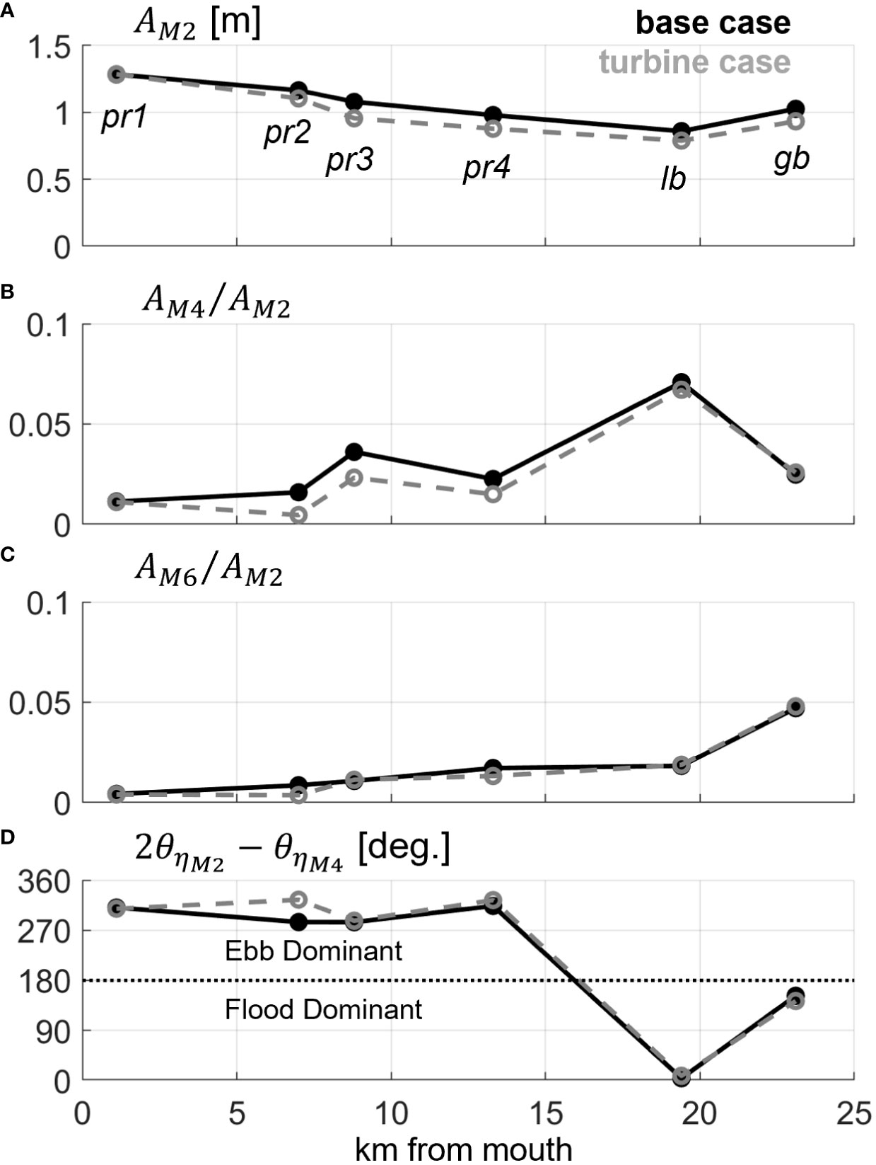
Figure 10 Along-estuary (x-axis) variability in free surface tidal amplitudes and distortion for the base (black, solid) and turbine (gray, dashed) simulations. Shown from top to bottom are: M₂ amplitude (A), ratio of M₄ to M₂ amplitude (B), ratio of M₆ to M₂ amplitude (C), and the flood-ebb dominance phase relation between M₂ and M₄ (D). Sections are labeled in (A).

It is also important to remark on the relative magnitude of the M₆ overtide versus the M₄. Here, we see that $\raisebox{1ex}{$A_{M6}$}\!\left/ \!\raisebox{-1ex}{$A_{M2}$}\right.$ only exceeds $\raisebox{1ex}{$A_{M4}$}\!\left/ \!\raisebox{-1ex}{$A_{M2}$}\right.$ at section gb (Figure 10C), which indicates quadratic friction only becomes more important than the asymmetric nonlinear mechanisms in the shallow tidal flats within Great Bay. This trend is unchanged with or without turbines simulated, implying turbines have a greater influence on the asymmetric mechanisms associated with M₄ than quadratic friction. Moreover, considering friction dominates nonlinear distortions in Great Bay, the location where tidal distortion is modified the least, it is likely that nonlinear mechanisms other than friction (i.e., intertidal storage) controlling downstream asymmetries are more sensitive to the presence of turbines. We explore this concept further in the next section, where we quantify spatial variability in the major asymmetric nonlinear mechanisms and identify how tidal turbines modify each.

4.3 Intertidal storage and frictional effects

In their notable paper on the topic, Friedrichs and Aubrey (1988) identified how the relative magnitudes of simple scaling ratios for depth-dependent friction and estuary geometry indicate whether an estuary region is flood or ebb dominant and the strength of that dominance. Flood dominance has been found to always occur for $a/h>0.3$, with the magnitude of flood dominance increasing with $a/h$. Alternatively, ebb dominance occurs when $a/h<0.3$ and smaller than $V_s/V_c$ (intertidal storage volume/channel storage volume at low water). Should that condition be met, the strength of ebb asymmetry increases with $V_s/V_c$ (Friedrichs and Aubrey, 1988). Being a geometrically complex estuarine system which we identify as being ebb (flood) dominant in the Piscataqua River (Great Bay), there clearly is along-estuary variability in both nonlinear forcing mechanisms (Figure 10), but it remains unclear the relative importance of depth-dependent friction to intertidal storage spatially or how energy extraction modifies the terms. In this section, we address how the nonlinear physical mechanisms which control tidal transport and asymmetry are modulated by tidal energy extraction.

The scaled representation of intertidal storage, $\raisebox{1ex}{$V_s$}\!\left/ \!\raisebox{-1ex}{$V_c$}\right.$, becomes less important as the volume of water between low and high tides in the estuary ($V_s$) decreases relatively more than the low water submerged channel volumes ($V_c$). In an estuary with extensive tidal flat zones such at the PRGB system, changes to intertidal areas and tidal prisms are good indicators of this term (Figure 11). Intertidal area, $A_i$, was calculated for each tide over a spring-neap cycle as the difference in wetted area between high and low waters. Similarly, tidal prism, P, quantifies the volume of water stored in the estuary between low and high waters and was calculated as a time integral of the volume flux, Q, through the mouth (section pr1) during each flood tide:

FIGURE 11

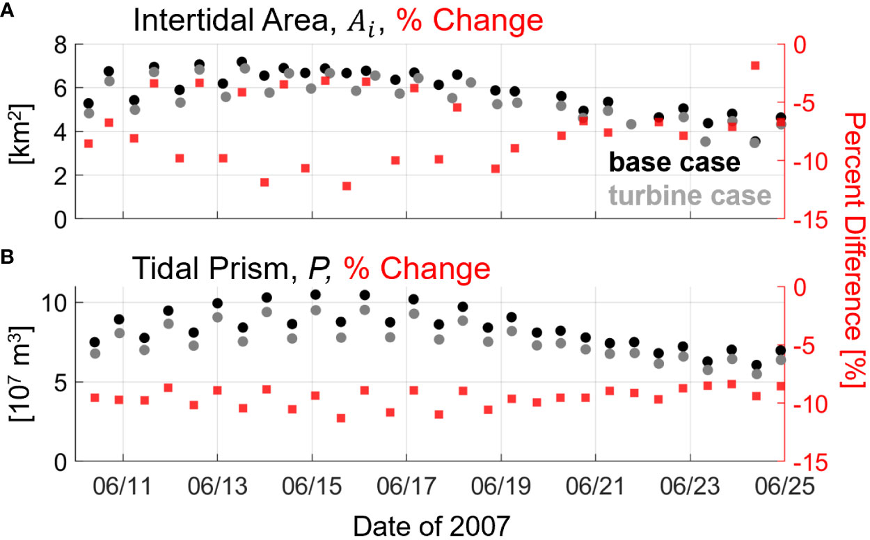
Figure 11 Time series of total estuary intertidal area (A) and tidal prism (B) for each tidal cycle over a 15-day spring-neap cycle, with areas and volumes on the left-hand-side y-axes. Percent differences between turbine and base cases are given as red squares and correspond to the right-hand-side y-axes. X-axis is date in 2007.

$\begin{array}{ll}P=\underset{t_{lw}}{\overset{t_{hw}}{\int }}Q dt& (12)\end{array}$

where $t_{lw}$ and $t_{hw}$ are the times of low and high waters, respectively. In the base simulation, $A_i$ varies from 4 to 7 km² between neap and spring tides, respectively, illustrating the extent of the tidal flat zones in the PRGB estuary as well as the significant fortnightly variability (area nearly doubles from neap to spring, Figure 11A). When turbines are modeled, $A_i$ is reduced by ~6% during neap tides and up to ~12% during springs (Figure 11A), a direct effect of reduced tidal ranges upstream of the turbines (Figure 10A). Interestingly, the largest spring tides see some of the smallest decreases in intertidal area (<5%), likely because both the base and turbine simulations are reaching the maximum tidal flat coverage possible, so differences in high water marks beyond that point do not matter. More consistent variability is reflected in P, as the maximum tidal flat area is not a limiting factor (i.e., P can continue to increase after $A_i$ maximizes). During the base run, P maximizes near 1.0x10⁸ m³ (spring tides) and minimizes at 7.0x10⁷ m³ (neap). After adding turbines, P is reduced 8% to 10% during neap tides and 8% to 12% during spring tides (Figure 11B). These order of magnitude reductions in tidal prism throughout the fortnightly period point to a correspondingly significant effect on the intertidal storage mechanism which drives ebb dominance, and likely insignificant variability over the spring-neap cycle.

To confirm the nonlinear intertidal storage mechanism is reduced, quantify the relative importance of nonlinear depth-dependent friction, and identify along-estuary variability in the mechanisms, $\raisebox{1ex}{$V_s$}\!\left/ \!\raisebox{-1ex}{$V_c$}\right.$ and $\raisebox{1ex}{$a$}\!\left/ \!\raisebox{-1ex}{$h$}\right.$ were quantified at each section for the base and turbine runs. $V_s$ was calculated similar to that in Friedrichs and Aubrey (1988):

$\begin{array}{ll}{V}_s=P-\overline{2a}{A}_s& (13)\end{array}$

where P is the tidal prism landward of the section (Equation 12), a is the M₂ tidal amplitude, and $A_s$ is the low water channel surface area landward of the section, with overbars denoting a spatial average between the given section and estuary head. $V_c$ was then estimated as the mean sea level channel volumes between the section and estuary head (Squamscott River outlet in Great Bay, Figure 1) while h is the mean depth across the section.

In the base simulation, $\raisebox{1ex}{$V_s$}\!\left/ \!\raisebox{-1ex}{$V_c$}\right.$ increases from 0.35 at the estuary mouth to 1.4 in Great Bay, as the relative volume of submerged channels to tidal storage is decreased moving upstream, subsequently scaling up the intertidal storage mechanism (Figure 12). $\raisebox{1ex}{$a$}\!\left/ \!\raisebox{-1ex}{$h$}\right.$ generally increases moving landward but remains significantly smaller in magnitude and only exceeds 0.3 in Great Bay (Figure 12), where mean depths are shallowest, confirming that depth-dependent friction is the principal nonlinear mechanism modulating distortion there and contributing to the flood dominance previously outlined (Figures 9, 10). Downstream, $\raisebox{1ex}{$a$}\!\left/ \!\raisebox{-1ex}{$h$}\right.$ remains below 0.3 as the tidal amplitude is largely similar but the channel sections are deeper and lacking in shallow shoals or tidal flats. $\raisebox{1ex}{$V_s$}\!\left/ \!\raisebox{-1ex}{$V_c$}\right.$ well exceeds $\raisebox{1ex}{$a$}\!\left/ \!\raisebox{-1ex}{$h$}\right.$ downstream of Great Bay, verifying nonlinear intertidal storage as the mechanism dictating tidal distortion creating ebb dominance (Figures 9, 10). In between at Little Bay, $\raisebox{1ex}{$a$}\!\left/ \!\raisebox{-1ex}{$h$}\right.$ is nearest to 0.3, suggesting neither frictional nor intertidal storage dominance. Adding tidal energy extraction to the model principally effects $\raisebox{1ex}{$V_s$}\!\left/ \!\raisebox{-1ex}{$V_c$}\right.$, reducing the ratio quite consistently by 20% to 25% system-wide (Figure 12). Alternatively, $\raisebox{1ex}{$a$}\!\left/ \!\raisebox{-1ex}{$h$}\right.$ is mainly unchanged, and only slightly decreased at lb (< 5%) and gb (< 10%, Figure 12). Regardless of reductions in $\raisebox{1ex}{$V_s$}\!\left/ \!\raisebox{-1ex}{$V_c$}\right.$ at gb, $\raisebox{1ex}{$a$}\!\left/ \!\raisebox{-1ex}{$h$}\right.$ remains larger than 0.3 in both simulations, allowing flood dominance to persist.

FIGURE 12

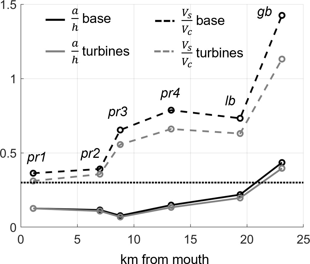
Figure 12 Comparison of scaled nonlinear friction ($\raisebox{1ex}{$a$}\!\left/ \!\raisebox{-1ex}{$h$}\right.$, solid lines) and intertidal storage ($\raisebox{1ex}{$V_s$}\!\left/ \!\raisebox{-1ex}{$V_c$}\right.$, dashed lines) terms (y-axis) along estuary (x-axis). Black lines denote base case and gray indicate turbine simulation. The horizontal dotted line highlights 0.3 on the y-axis. Sections are labeled.

Ultimately, we see that tidal energy extraction reduces ebb-dominant asymmetry in the channelized, Piscataqua River sections of the estuary by decreasing intertidal storage (Figure 11), thereby dampening the influence of the associated nonlinear mechanism (Figure 12). Reduced intertidal storage is a result of turbines decreasing the tidal range upstream of the farm (Figure 10), an effect indicative of increased linear frictional damping on the tidal wave. In flood-dominant Great Bay, depth-dependent friction controls asymmetry but is not meaningfully modified by tidal energy extraction (Figure 12), so little change is seen in tidal distortion (Figures 9, 10). We suspect that fortnightly variability to these processes is relatively small based on the consistent spring-neap variability in tidal prism shown in Figure 11 but is a topic worthy of future investigation. Further, these results highlight the disproportionate effects of reduced tidal ranges on tidal asymmetry mechanisms when significant tidal flat storage is possible: relatively minor reductions to the tidal amplitude (in this case, ~10 cm, Figure 10A) lead to correspondingly minor reductions in depth-dependent friction (<10%), but when acting over intertidal areas on the order of 6 km² (Figure 11A), can reduce the inflowing tidal volume by ~10⁷ m³ (Figure 11B) and nonlinear intertidal storage up to 25%. At the most basic level, changes to tidal flat wetting and drying areas dictate the hydrodynamical changes outlined in this paper.

5 Discussion

This work outlines ways in which energy extraction via a synthetic tidal stream turbine farm may alter tidal hydrodynamics in the PRGB estuary, a well-mixed system. Here, we consider some possible impacts on estuarine health and sediment transport, applicability to other systems, and future research pathways.

5.1 Ecological and environmental considerations

A primary process generally associated with tidal asymmetry is sediment transport. In ebb dominant regions, bed load sediment is generally flushed seaward, eventually out of the estuary, and usually creates a morphologically stable system. In flood dominant zones, coarse sediment is flushed landward and tends to infill channels, typically resulting in more complex and time varying morphologies (e.g., Speer and Aubrey, 1985; Friedrichs and Aubrey, 1988). Similarly, more fine scale, suspended particulate matter (SPM) is sensitive to tidal transport asymmetries, a type of SPM transport deemed “tidal pumping” which influences the location of estuary turbidity maxima (ETM) and correspondingly degraded water quality (e.g., Uncles et al., 1985; Scully and Friedrichs, 2007). Alterations to flood or ebb dominance therefore have immediate impacts on sediment erosion, deposition, and morphology (e.g., Xie et al., 2009), as well as spatial variation in turbidity. This work indicates a weakening of seaward sediment transport seaward of Great Bay is likely if tidal turbines are installed. Decreased ebb-directed transport (Figure 9) could presumably reduce erosion efficiency within the Piscataqua River channel, allow some deposition of coarse SPM previously held suspended under stronger currents, and generally increase sediment export timescales from the estuary. Shoaling of coarse sediments in the Piscataqua River channel has been a problem in the past: sand waves up to 3 m in height form at a rate of 0.3 m/year and are periodically dredged for navigational purposes (Bilgili et al., 2003). Although the source of sands producing the waves is not confirmed, Bilgili et al. (2003) suggest an upstream (landward) source, as there is low sand availability near the mouth and the net bed-load transport is seaward directed in the Piscataqua River. It is therefore possible this sedimentation could worsen or begin to occur in previously unaffected areas if a large number of turbines are deployed and landward sand sources are less effectively transported out of the estuary. Conversely, the general weakening of tidal currents (Figure 6) could also reduce ETM concentrations as less sediment will be resuspended, perhaps locally improving water quality. The ETM in the PRGB estuary is always present in Great Bay and varies in concentration from roughly 4 to 13 mg suspended sediment/liter depending on discharge and wind conditions (Ward and Bub, 2005). Both topics are important to consider and study further prior to turbine installation.

In recent decades, the PRGB estuary has experienced an alarming decline in eelgrass volume: 35% since 1996 (Short, 2012). Eelgrass biomass is an indicator of estuarine health worldwide (Orth et al., 2006; Waycott et al., 2009), considered to be the basis of estuarine food webs, and supports many recreationally, commercially, and ecologically important species both within and outside the PRGB system. Local decline in the PRGB estuary is mainly attributed to degrading water quality caused by excessive micro/macroalgal growth and turbidity (Short, 2012; Bricker et al., 2020). Algal growth occurs due to “moderately high” eutrophic conditions in the estuary caused by low dissolved oxygen and excessive nitrogen loading from runoff and groundwater (PREP, 2013; Bricker et al., 2015; PREP, 2018). It is possible adding a large tidal energy turbine array (such as the synthetic one in this work) to the system could further impact eelgrass in the estuary. Physically, we show residual flows out of the estuary will be reduced (Figure 7), possibly slowing nitrogen export. We do not quantify or discuss mixing in this study, but former work has shown locally enhanced vertical mixing in the vicinity of turbines can be beneficial to dissolved oxygen and water quality (Wang et al., 2015), potentially helping eelgrass and other water quality metrics in the PRGB estuary. Further, the relatively significant reductions in intertidal area anticipated following turbine deployment (Figure 11) will simply decrease the total area favorable for eelgrass growth, which tends to favor shallow intertidal and subtidal zones. Shellfish harvesting (clams, oysters) is also popular in the PRGB system (PREP, 2018). Reduced intertidal area could decrease shellfish habitat and harvesting opportunities. More research is warranted on all these topics, which are presented here for future investigators to consider.

5.2 Broader applicability

Although this study is based in the PRGB estuary, the results have broad applicability to other shallow, well-mixed systems common globally. In other ebb dominant estuaries with tidal asymmetry controlled by nonlinear intertidal storage ($\raisebox{1ex}{$V_s$}\!\left/ \!\raisebox{-1ex}{$V_c$}\right.>\raisebox{1ex}{$a$}\!\left/ \!\raisebox{-1ex}{$h$}\right.<0.3$), we expect tidal turbine impacts to largely replicate these results: intertidal storage volumes will be reduced, ebb transport diminished more than flood, and decreased overall tidal asymmetry. In flood dominant estuaries where depth dependent friction controls ($\raisebox{1ex}{$a$}\!\left/ \!\raisebox{-1ex}{$h$}\right.>0.3$ or $0.3>\raisebox{1ex}{$a$}\!\left/ \!\raisebox{-1ex}{$h$}\right.>\raisebox{1ex}{$V_s$}\!\left/ \!\raisebox{-1ex}{$V_c$}\right.$), we anticipate flood asymmetry to be weakened due to decreases tidal amplitudes, but to a lesser extent relative to intertidal storage modulation on ebb dominance. That said, in very shallow systems (more so than the PRGB estuary) with average tidal amplitudes near channel depths ($\raisebox{1ex}{$a$}\!\left/ \!\raisebox{-1ex}{$h$}\right.\sim 1$) and significant frictional distortion, reductions to tidal amplitude could have more profound effects on asymmetry and transport. Moreover, systems with near equal contributions from nonlinear intertidal storage and depth dependent friction to asymmetric distortion could experience shifts from flood to ebb dominance (or vice versa). Although this change in asymmetry regime was found unlikely to occur in the PRGB estuary, it is entirely possible this could happen elsewhere and would have more profound impacts on residual circulation, sediment transport, and morphological stability than the findings presented here. These speculations outline important topics to pursue in future research on tidal energy extraction in shallow, well-mixed estuaries.

6 Conclusions

Tidal energy extraction via a large, synthetic tidal turbine farm has the potential to modulate tidal asymmetry and transport in a shallow, well-mixed estuary. The estuary features asymmetric tidal dynamics and is mainly ebb dominant in the deeper, channelized sections from the mouth to mid-reaches, and slightly flood dominant upstream in a significant shallow, tidal flat region. Modeled tidal turbines near the mouth act as momentum sinks and effectively increase the linear effect of friction on the landward propagating tidal wave, reducing the free surface amplitude. Moreover, the relative magnitude of nonlinear tidal distortion is reduced in the ebb-dominant zones, creating a less asymmetric tidal wave than typical. As such, tidal currents and transport are reduced during both tidal phases but are diminished relatively more on ebb tides in the ebb dominant sections. The relative importance of nonlinear shallow water/friction to nonlinear intertidal storage mechanisms are evaluated to identify physical controls on the spatially varying asymmetric decreases in transport. It is found that relatively modest reductions in tidal amplitude (~10 cm or ~10% of typical amplitude) significantly lower the storage capacity of upstream tidal flats by ~10⁷ m³ and directly reduces the nonlinear intertidal storage mechanism, which dictates the strength of ebb dominance downstream, up to 25%. Nonlinear depth-dependent friction, which controls the magnitude of flood dominance, is only important upstream in the flats and is reduced generally less than 10% with turbines.

As such, we identify reductions to estuary intertidal area and volume, important physical controls on tidal asymmetry and transport, as a major result of tidal energy extraction in shallow well-mixed estuaries. It is likely the importance of this mechanism varies system-to-system and depends on the interplay between intertidal storage capacities and friction. Although we saw no regime changes from flood to ebb dominance (or vice versa), it is possible this could happen in other systems and would have important implications on sediment and material transport. We outline some environmental metrics associated with tidal energy extraction induced changes to transport which coastal planners should consider prior to turbine deployments.

Data availability statement

The raw data supporting the conclusions of this article will be made available by the authors, without undue reservation.

Author contributions

PS: Conceptualization, Data curation, Formal Analysis, Investigation, Methodology, Validation, Visualization, Writing – original draft, Writing – review and editing. ZY: Conceptualization, Funding acquisition, Methodology, Project administration, Supervision, Validation, Writing – review and editing. TW: Data curation, Software, Writing – review and editing. MD: Data curation, Software, Writing – review and editing.

Funding

The authors declare financial support was received for the research, authorship, and/or publication of this article. This study was funded by the U.S. Department of Energy, Office of Energy Efficiency and Renewable Energy, Water Power Technologies Office under contract DE-AC05-76RL01830 at the Pacific Northwest National Laboratory (PNNL).

Acknowledgments

All model simulations were performed using PNNL’s Institutional Computing facility and NREL’s Eagle Computing System. All colormaps were created with the cmocean MATLAB toolbox (Thyng et al., 2016). The authors would like to thank Tom Lippmann and Larry Ward at UNH for helping us compile the relevant bathymetry datasets. We also thank the two reviewers whose comments improved the original manuscript.

Conflict of interest

The authors declare that the research was conducted in the absence of any commercial or financial relationships that could be construed as a potential conflict of interest.

Publisher’s note

All claims expressed in this article are solely those of the authors and do not necessarily represent those of their affiliated organizations, or those of the publisher, the editors and the reviewers. Any product that may be evaluated in this article, or claim that may be made by its manufacturer, is not guaranteed or endorsed by the publisher.

References

Bilgili A., Swift M. R., Lynch D. R., Ip J. T. C. (2003). Modeling bed-load transport of coarse sediments in the Great Bay Estuary, New Hampshire. Estuarine Coast. Shelf Sci. 58 (4), 937–950. doi: 10.1016/j.ecss.2003.07.007

CrossRef Full Text | Google Scholar

Boon J. D., Byrne R. J. (1981). On basin hypsometry and the morphodynamic response of coastal inlet systems. Mar. Geology 40 (1/2), 27–48. doi: 10.1016/0025-3227(81)90041-4

CrossRef Full Text | Google Scholar

Bricker S. B., Ferreira J., Zhu C., Rose J. M., Galimany E., Wikfors G. H., et al. (2015). An ecosystem services assessment using bioextraction technologies for removal of nitrogen and other substances in Long Island Sound and the Great Bay/Piscataqua Region Estuaries NOAA Technical Memorandum NOS NCCOS 194. Silver Spring, MD. 154 pp + 3 appendices. doi: 10.25923/pw15-kx66

CrossRef Full Text | Google Scholar

Bricker S. B., Grizzle R. E., Trowbridge P., Rose J. M., Ferreira J. G., Wellman K., et al. (2020). Bioextractive removal of nitrogen by oysters in great bay piscataqua river estuary, New Hampshire, USA. Estuaries Coasts 43 (1), 23–38. doi: 10.1007/s12237-019-00661-8

PubMed Abstract | CrossRef Full Text | Google Scholar

Brown J. M., Davies A. G. (2010). Flood/ebb tidal asymmetry in a shallow sandy estuary and the impact on net sand transport. Geomorphology 114 (3), 431–439. doi: 10.1016/j.geomorph.2009.08.006

CrossRef Full Text | Google Scholar

Brown W. S., Trask R. P. (1980). A study of tidal energy-dissipation and bottom stress in an estuary. J. Phys. Oceanography 10 (11), 1742–1754. doi: 10.1175/1520-0485(1980)010<1742:Asoted>2.0.Co;2

CrossRef Full Text | Google Scholar

Burchard H., Schuttelaars H. M., Ralston D. K. (2018). Sediment trapping in estuaries. Annu. Rev. Mar. Sci. 10 (1), 371–395. doi: 10.1146/annurev-marine-010816-060535

CrossRef Full Text | Google Scholar

Chen C., Liu H., Beardsley R. C. (2003). An unstructured grid, finite-volume, three-dimensional, primitive equations ocean model: Application to coastal ocean and estuaries [Article]. J. Atmospheric Oceanic Technol. 20 (1), 159–186. doi: 10.1175/1520-0426(2003)020<0159:AUGFVT>2.0.CO;2

CrossRef Full Text | Google Scholar

Codiga D. L. (2011) Unified Tidal Analysis and Prediction Using the UTide Matlab Functions. Available at: ftp://www.po.gso.uri.edu/pub/downloads/codiga/pubs/2011Codiga-UTide-Report.pdf.

Google Scholar

Cook S. E., Lippmann T. C., Irish J. D. (2019). Modeling nonlinear tidal evolution in an energetic estuary. Ocean Model. 136, 13–27. doi: 10.1016/j.ocemod.2019.02.009

CrossRef Full Text | Google Scholar

Cowles G. W., Hakim A. R., Churchill J. H. (2017). A comparison of numerical and analytical predictions of the tidal stream power resource of Massachusetts, USA. Renewable Energy 114, 215–228. doi: 10.1016/j.renene.2017.05.003

CrossRef Full Text | Google Scholar

Deb M., Yang Z., Haas K. A., Wang T. (in review). Hydrokinetic tidal energy resource assessment following international electrotechnical commission guidelines. Renewable Sustain. Energy Rev.

Google Scholar

De Dominicis M., O'Hara Murray R., Wolf J. (2017). Multi-scale ocean response to a large tidal stream turbine array. Renewable Energy 114, 1160–1179. doi: 10.1016/j.renene.2017.07.058

CrossRef Full Text | Google Scholar

Díaz H., Rodrigues J., Soares C. G. (2020). Preliminary assessment of a tidal test site on the Minho estuary. Renewable Energy 158, 642–655. doi: 10.1016/j.renene.2020.05.072

CrossRef Full Text | Google Scholar

Dronkers J. (1986). Tidal asymmetry and estuarine morphology. Netherlands J. Sea Res. 20 (2), 117–131. doi: 10.1016/0077-7579(86)90036-0

CrossRef Full Text | Google Scholar

Egbert G. D., Erofeeva S. Y. (2002). Efficient inverse modeling of barotropic ocean tides. J. Atmospheric Oceanic Technol. 19 (2), 183–204. doi: 10.1175/1520-0426(2002)019<0183:Eimobo>2.0.Co;2

CrossRef Full Text | Google Scholar

Ertürk Ş.N., Bilgili A., Swift M. R., Brown W. S., Çelikkol B., Ip J. T. C., et al. (2002). Simulation of the Great Bay Estuarine System: Tides with tidal flats wetting and drying. J. Geophysical Research: Oceans 107 (C5), 6–1-6-10. doi: 10.1029/2001JC000883

CrossRef Full Text | Google Scholar

Friedrichs C. T., Aubrey D. G. (1988). Non-linear tidal distortion in shallow well-mixed estuaries: a synthesis. Estuarine Coast. Shelf Sci. 27 (5), 521–545. doi: 10.1016/0272-7714(88)90082-0

CrossRef Full Text | Google Scholar

Gao G. D., Wang X. H., Bao X. W. (2014). Land reclamation and its impact on tidal dynamics in Jiaozhou Bay, Qingdao, China. Estuarine Coast. shelf Sci. 151, 285–294. doi: 10.1016/j.ecss.2014.07.017

CrossRef Full Text | Google Scholar

Garrett C., Cummins P. (2005). The power potential of tidal currents in channels. Proc. R. Soc. A: Mathematical Phys. Eng. Sci. 461 (2060), 2563–2572. doi: 10.1098/rspa.2005.1494

CrossRef Full Text | Google Scholar

Godin G. (1986). The use of nodal corrections in the calculation of harmonic constants. Int. Hydrographic Review. 63, 2. Available at: https://journals.lib.unb.ca/index.php/ihr/article/view/23428.

Google Scholar

Hasegawa D., Sheng J., Greenberg D. A., Thompson K. R. (2011). Far-field effects of tidal energy extraction in the Minas Passage on tidal circulation in the Bay of Fundy and Gulf of Maine using a nested-grid coastal circulation model. Ocean Dynamics 61, 1845–1868. doi: 10.1007/s10236-011-0481-9

CrossRef Full Text | Google Scholar

Haverson D., Bacon J., Smith H. C. M., Venugopal V., Xiao Q. (2018). Modelling the hydrodynamic and morphological impacts of a tidal stream development in Ramsey Sound. Renewable Energy 126, 876–887. doi: 10.1016/j.renene.2018.03.084

CrossRef Full Text | Google Scholar

IEC. (2015). Technical Specification: Marine energy - Wave, tidal and other water current converters - Part 201: Tidal energy resource assessment and characterization 62600-201, 44.

Google Scholar

Ip J. T. C., Lynch D. R., Friedrichs C. T. (1998). Simulation of estuarine flooding and dewatering with application to great Bay, New Hampshire. Estuarine Coast. Shelf Sci. 47 (2), 119–141. doi: 10.1006/ecss.1998.0352

CrossRef Full Text | Google Scholar

Jay D. A., Musiak J. D. (1996). “Internal Tidal Asymmetry in Channel Flows: Origins and Consequences,” in Mixing Processes in Estuaries and Coastal Seas, vol. 50 . Ed. Pattiaratchi C. (American Geophysical Union), 211–249.

Google Scholar

Khanjanpour M. H., Javadi A. A. (2020). Optimization of the hydrodynamic performance of a vertical Axis tidal (VAT) turbine using CFD-Taguchi approach. Energy Conversion Manage. 222, 113235. doi: 10.1016/j.enconman.2020.113235

CrossRef Full Text | Google Scholar

Li X., Li M., McLelland S. J., Jordan L.-B., Simmons S. M., Amoudry L. O., et al. (2017). Modelling tidal stream turbines in a three-dimensional wave-current fully coupled oceanographic model. Renewable Energy 114, 297–307. doi: 10.1016/j.renene.2017.02.033

CrossRef Full Text | Google Scholar

Lieberthal B., Huguenard K., Ross L., Bears K. (2019). The generation of overtides in flow around a headland in a low inflow estuary. J. Geophysical Research: Oceans 124 (2), 955–980. doi: 10.1029/2018jc014039

CrossRef Full Text | Google Scholar

McLaughlin J. W., Bilgili A., Lynch D. R. (2003). Numerical modeling of tides in the Great Bay Estuarine System: dynamical balance and spring–neap residual modulation. Estuarine Coast. Shelf Sci. 57 (1), 283–296. doi: 10.1016/S0272-7714(02)00355-4

CrossRef Full Text | Google Scholar

Neill S. P., Haas K. A., Thiébot J., Yang Z. (2021). A review of tidal energy—Resource, feedbacks, and environmental interactions. J. Renewable Sustain. Energy 13 (6). doi: 10.1063/5.0069452

CrossRef Full Text | Google Scholar

Neill S. P., Litt E. J., Couch S. J., Davies A. G. (2009). The impact of tidal stream turbines on large-scale sediment dynamics. Renewable Energy 34 (12), 2803–2812. doi: 10.1016/j.renene.2009.06.015

CrossRef Full Text | Google Scholar

O’Hara Murray R., Gallego A. (2017). A modelling study of the tidal stream resource of the Pentland Firth, Scotland. Renewable Energy 102, 326–340. doi: 10.1016/j.renene.2016.10.053

CrossRef Full Text | Google Scholar

Orth R. J., Carruthers T. J. B., Dennison W. C., Duarte C. M., Fourqurean J. W., Heck K. L., et al. (2006). A global crisis for seagrass ecosystems. BioScience 56 (12), 987–996. doi: 10.1641/0006-3568(2006)56[987:Agcfse]2.0.Co;2

CrossRef Full Text | Google Scholar

Parker B. B. (1984). Frictional effects on the tidal dynamics of a shallow estuary (Baltimore, MD: John Hopkins University).

Google Scholar

Parker B. B. (1991). Tidal Hydrodynamics (New York: John Wiley and Sons, Inc).

Google Scholar

PREP. (2013). State of our Estuaries 2013 (Durham, NH: PREP Reports and Publications). Available at: https://scholars.unh.edu/prep/259/.

Google Scholar

PREP. (2018). State of our Estuaries 2018 (PREP Reports and Publications). Available at: https://scholars.unh.edu/prep/391/.

Google Scholar

Qian P., Feng B., Liu H., Tian X., Si Y., Zhang D. (2019). Review on configuration and control methods of tidal current turbines. Renewable Sustain. Energy Rev. 108, 125–139. doi: 10.1016/j.rser.2019.03.051

CrossRef Full Text | Google Scholar

Rao S., Xue H., Bao M., Funke S. (2016). Determining tidal turbine farm efficiency in the Western Passage using the disc actuator theory. Ocean Dynamics 66 (1), 41–57. doi: 10.1007/s10236-015-0906-y

CrossRef Full Text | Google Scholar

Ross L., Alahmed S., Smith S. M. C., Roberts G. (2021). Tidal and subtidal transport in short, tidally-driven estuaries with low rates of freshwater input. Continental Shelf Res. 224, 104453. doi: 10.1016/j.csr.2021.104453

CrossRef Full Text | Google Scholar

Ross L., Valle-Levinson A., Sottolichio A., Huybrechts N. (2017). Lateral variability of subtidal flow at the mid-reaches of a macrotidal estuary. J. Geophysical Research: Oceans 122 (9), 7651–7673. doi: 10.1002/2016jc012504

CrossRef Full Text | Google Scholar

Sánchez M., Carballo R., Ramos V., Iglesias G. (2014). Tidal stream energy impact on the transient and residual flow in an estuary: A 3D analysis. Appl. Energy 116, 167–177. doi: 10.1016/j.apenergy.2013.11.052

CrossRef Full Text | Google Scholar

Scully M. E., Friedrichs C. T. (2007). Sediment pumping by tidal asymmetry in a partially mixed estuary. J. Geophysical Research: Oceans 112 (C7). doi: 10.1029/2006JC003784

CrossRef Full Text | Google Scholar

Short F. T. (1992). The ecology of the Great Bay Estuary, New Hampshire and Maine: an estuarine profile and bibliography. Available at: https://scholars.unh.edu/prep/376.

Google Scholar

Short F. T. (2012). Eelgrass Distribution in the Great Bay Estuary for 2011 (Durham NH: PREP Reports and Publications). Available at: https://scholars.unh.edu/prep/3.

Google Scholar

Speer P. E., Aubrey D. G. (1985). A study of non-linear tidal propagation in shallow inlet/estuarine systems Part II: Theory. Estuarine Coast. Shelf Sci. 21 (2), 207–224. doi: 10.1016/0272-7714(85)90097-6

CrossRef Full Text | Google Scholar

Speer P. E., Aubrey D. G., Friedrichs C. T. (1991). Nonlinear hydrodynamics of shallow tidal inlet/bay systems. Tidal hydrodynamics 321, 339.

Google Scholar

Suh S. W., Lee H. Y., Kim H. J. (2014). Spatio-temporal variability of tidal asymmetry due to multiple coastal constructions along the west coast of Korea. Estuarine Coast. Shelf Sci. 151, 336–346. doi: 10.1016/j.ecss.2014.09.007

CrossRef Full Text | Google Scholar

Swift M. R., Brown W. S. (1983). Distribution of bottom stress and tidal energy-dissipation in a well-mixed estuary. Estuar. Coast. Shelf Sci. 17 (3), 297–317. doi: 10.1016/0272-7714(83)90024-0

CrossRef Full Text | Google Scholar

Talke S. A., Jay D. A. (2020). Changing tides: the role of natural and anthropogenic factors. Annu. Rev. Mar. Sci. 12 (1), 121–151. doi: 10.1146/annurev-marine-010419-010727

CrossRef Full Text | Google Scholar

Thyng K. M., Greene C. A., Hetland R. D., Zimmerle H. M., DiMarco S. F. (2016). True colors of oceanography: Guidelines for effective and accurate colormap selection. Oceanography 29 (3), 9–13. doi: 10.5670/oceanog.2016.66

CrossRef Full Text | Google Scholar

Trowbridge P. (2007). Hydrological Parameters for New Hampshire's Estuaries (Durham NH: PREP Reports and Publications). Available at: https://scholars.unh.edu/prep/130/.

Google Scholar

Uncles R. J. (1981). A note on tidal asymmetry in the severn estuary. Estuarine Coast. Shelf Sci. 13 (4), 419–432. doi: 10.1016/S0302-3524(81)80038-2

CrossRef Full Text | Google Scholar

Uncles R. J., Elliott R. C. A., Weston S. A. (1985). Observed fluxes of water, salt and suspended sediment in a partly mixed estuary. Estuarine Coast. shelf Sci. 20 (2), 147–167. doi: 10.1016/0272-7714(85)90035-6

CrossRef Full Text | Google Scholar

U.S.A.C.E. (2014). Portsmouth harbor and piscataqua river Portsmouth, New Hampshire: Navigation improvement project feasibility study: appendix C.

Google Scholar

Vazquez A., Iglesias G. (2015). Device interactions in reducing the cost of tidal stream energy. Energy Conversion Manage. 97, 428–438. doi: 10.1016/j.enconman.2015.03.044

CrossRef Full Text | Google Scholar

Vazquez A., Iglesias G. (2016). Capital costs in tidal stream energy projects–A spatial approach. Energy 107, 215–226. doi: 10.1016/j.energy.2016.03.123

CrossRef Full Text | Google Scholar

Wang T., Yang Z. (2017). A modeling study of tidal energy extraction and the associated impact on tidal circulation in a multi-inlet bay system of Puget Sound. Renewable Energy 114, 204–214. doi: 10.1016/j.renene.2017.03.049

CrossRef Full Text | Google Scholar

Wang T., Yang Z., Copping A. (2015). A modeling study of the potential water quality impacts from in-stream tidal energy extraction. Estuaries Coasts 38 (S1), 173–186. doi: 10.1007/s12237-013-9718-9

CrossRef Full Text | Google Scholar

Ward L. G., Bub F. L. (2005). “Temporal Variability in Salinity, Temperature and Suspended Sediments in a Gulf of Maine Estuary (Great Bay Estuary, New Hampshire,” in High Resolution Morphodynamics and Sedimentary Evolution of Estuaries. Eds. FitzGerald D. M., Knight J. (Netherlands: Springer), 115–142. doi: 10.1007/1-4020-3296-X_7

CrossRef Full Text | Google Scholar

Ward S. L., Green J. A. M., Pelling H. E. (2012). Tides, sea-level rise and tidal power extraction on the European shelf. Ocean Dynamics 62 (8), 1153–1167. doi: 10.1007/s10236-012-0552-6

CrossRef Full Text | Google Scholar

Ward L. G., Johnson P., Bogonko M., McAvoy Z. S., Morrison R. C. (2021). Northeast Bathymetry and Backscatter Compilation: Western Gulf of Maine, Southern New England, and Long Island (Durham NH: BOEM/New Hampshire Cooperative Agreement).

Google Scholar

Waycott M., Duarte C. M., Carruthers T. J. B., Orth R. J., Dennison W. C., Olyarnik S., et al. (2009). Accelerating loss of seagrasses across the globe threatens coastal ecosystems. Proc. Natl. Acad. Sci. 106 (30), 12377–12381. doi: 10.1073/pnas.0905620106

CrossRef Full Text | Google Scholar

Wengrove M. E., Foster D. L., Kalnejais L. H., Percuoco V., Lippmann T. C. (2015). Field and laboratory observations of bed stress and associated nutrient release in a tidal estuary. Estuar. Coast. Shelf Sci. 161, 11–24. doi: 10.1016/j.ecss.2015.04.005

CrossRef Full Text | Google Scholar

Wilson A. M., Morris J. T. (2012). The influence of tidal forcing on groundwater flow and nutrient exchange in a salt marsh-dominated estuary. Biogeochemistry 108 (1), 27–38. doi: 10.1007/s10533-010-9570-y

CrossRef Full Text | Google Scholar

Wollast R. (2003). “Biogeochemical Processes in Estuaries,” in Marine Science Frontiers for Europe. Eds. Wefer G., Lamy F., Mantoura F. (Berlin Heidelberg: Springer), 61–77. doi: 10.1007/978-3-642-55862-7_5

CrossRef Full Text | Google Scholar

Xia J., Falconer R. A., Lin B. (2010). Impact of different operating modes for a Severn Barrage on the tidal power and flood inundation in the Severn Estuary, UK. Appl. Energy 87 (7), 2374–2391. doi: 10.1016/j.apenergy.2009.11.024

CrossRef Full Text | Google Scholar

Xie D., Wang Z., Gao S., De Vriend H. J. (2009). Modeling the tidal channel morphodynamics in a macro-tidal embayment, Hangzhou Bay, China. Continental Shelf Res. 29 (15), 1757–1767. doi: 10.1016/j.csr.2009.03.009

CrossRef Full Text | Google Scholar

Yang Z., Copping A. (2017). Marine renewable energy: Resource characterization and physical effects (Springer).

Google Scholar

Yang Z., Wang T. (2015). Modeling the effects of tidal energy extraction on estuarine hydrodynamics in a stratified estuary. Estuaries Coasts 38 (S1), 187–202. doi: 10.1007/s12237-013-9684-2

CrossRef Full Text | Google Scholar

Yang Z., Wang T., Branch R., Xiao Z., Deb M. (2021). Tidal stream energy resource characterization in the Salish Sea. Renewable Energy 172, 188–208. doi: 10.1016/j.renene.2021.03.028

CrossRef Full Text | Google Scholar

Yang Z., Wang T., Copping A. E. (2013). Modeling tidal stream energy extraction and its effects on transport processes in a tidal channel and bay system using a three-dimensional coastal ocean model. Renewable Energy 50, 605–613. doi: 10.1016/j.renene.2012.07.024

CrossRef Full Text | Google Scholar

Yang Z., Wang T., Copping A., Geerlofs S. (2014). Modeling of in-stream tidal energy development and its potential effects in Tacoma Narrows, Washington, USA. Ocean Coast. Manage. 99, 52–62. doi: 10.1016/j.ocecoaman.2014.02.010

CrossRef Full Text | Google Scholar