What data are needed to detect wildfire effects on coastal ecosystems? A case study during the Thomas Fire

Wildfires are growing in frequency and severity worldwide, with anthropogenic climate change predicted to worsen the effects of wildfires in the future. While most wildfire impacts occur on land, coastal fires can also affect the ocean via smoke production and ash deposition. The impacts of wildfires on marine ecology and biogeochemistry have been studied infrequently, as it is difficult to conduct fieldwork rapidly and safely during unpredictable natural disasters. Increasingly, remote sensing measurements are used to study the impacts of wildfires on marine ecosystems through optical proxies. Given the optical impacts of smoke and in-water ash, these measurements may be limited in their scope and accuracy. Here, we evaluate the potential and limitations of remote sensing data collected from MODIS-Aqua to describe the effects of wildfires on optics and phytoplankton observations. Using samples collected in the Santa Barbara Channel (California, USA) during the Thomas Fire in December 2017, we found that MODIS-Aqua data were unsuited for interpreting ecosystem effects during a wildfire. Our results identified a persistent overestimation of chlorophyll-a concentration from MODIS-Aqua compared to in situ measurements. Optical models applied to in situ radiometry data overestimated the absorption by colored dissolved organic matter (CDOM) during the wildfire. Satellites will remain an important tool to measure the impacts of wildfires on marine ecosystems, but this analysis demonstrates the importance of in situ sampling to quantify the impacts of wildfires on ocean ecology and biogeochemistry due to the difficulty of interpreting remote sensing data during these events.

1 Introduction

Around the world, wildfires are increasing in magnitude and severity (Doerr and Santín, 2016; Hamilton et al., 2018). The conditions that lead to more intense and destructive wildfires are also increasing, in part due to the effects of anthropogenic climate change on prolonged drought conditions and frequent severe weather events (Westerling et al., 2006). These impacts are particularly true in the western United States, where wildfire impacts on inland waters and watersheds have been studied (e.g., Coombs and Melack, 2013; Urmy et al., 2016). However, while wildfires are frequently proximal to the ocean, there have been few studies examining the impact of wildfires on the ecology and biogeochemistry of marine systems until recently. One example hypothesized about the impact of wildfire smoke on coral reef productivity in the near-coastal zone (e.g., Abram et al., 2003; van Woesik, 2004). Additional inferences about the influence of wildfire smoke and ash on the ocean have also been drawn from the parallel example of volcanic ash and smoke. Volcanic impacts have measurable effects on the ocean, including fertilizing the nutrient-limited open ocean (Duggen et al., 2007; Hamme et al., 2010).

Like volcanic eruptions, wildfires are largely unpredictable events. While some regions may be more susceptible to wildfires in certain seasons, the timing, duration, and extent of a potential fire is largely unknown prior to that event. Consequently, coastal studies are easier to conduct than open ocean approaches and can take advantage of existing nearshore time series to compare wildfire impacts to historical norms. Given the planning required to conduct a successful oceanographic research cruise, virtually no in situ studies existed to compare wildfire effects on ocean ecosystems prior to the Thomas Fire, which occurred during a pre-existing cruise (Bisson et al., 2020) and allowed for the evaluation of phytoplankton community composition during the fire (Kramer et al., 2020). Since then, other studies in the coastal ocean have examined the impacts of wildfires on dissolved black carbon (Wagner et al., 2021), on the concentrations of fecal indicator bacteria (Cira et al., 2022), and on dissolved organic matter deposition (Coward et al., 2022). These studies relied on the availability of ships to access the sampling sites during wildfires and collect samples on timescales relevant to the disaster, which can provide a further logistical and funding challenge.

Increasingly, satellite remote sensing provides a (near) real-time tool to monitor the impacts of these sporadic wildfire events on the open ocean, as has been done with volcanic impacts on the ocean (Westberry et al., 2019; Bisson et al., 2023; Franz et al., 2023). Both ocean color remote sensing and autonomous profiling floats (e.g., Argo) have been used as tools to identify phytoplankton blooms following a wildfire, particularly in inaccessible, open ocean and/or high-latitude regions (Ardyna et al., 2022; Wang et al., 2022; Weis et al., 2022). All three of these studies examined the changes in chlorophyll-a concentration and phytoplankton carbon indirectly through optical proxies and determined that wildfire smoke and ash is potentially fertilizing the Southern and Arctic Oceans, similarly to the effects observed after volcanic eruptions. Furthermore, these studies used business-as-usual satellite products and assumed those aerosol models and atmospheric corrections were appropriate, which may not be true during a wildfire. Given the unpredictable nature of wildfires on land and the potentially rapid response by phytoplankton in the coastal and open ocean, this area of study urgently requires further inquiry. However, the remote sensing component must be carefully considered to avoid drawing improper conclusions from ocean color imagery impacted by insufficient atmospheric correction or unexpected organic matter absorption and scattering.

It is highly likely that the proximal wildfire smoke and in situ ash affected remote sensing measurements and/or optical proxies employed in these previous studies, because smoke and ash obscure the ocean signal and provide challenges to conventional atmospheric correction. The majority (>90%) of the top-of-atmosphere radiance signal observed from passive satellites comes from atmospheric contributions. Even routine errors in atmospheric correction in the absence of smoke can create large downstream errors in ocean color products, and it has been demonstrated that errors in remote sensing reflectance ($R_{rs}(\lambda )$) are up to an order of magnitude larger than was previously understood in some regions (Bisson et al., 2021). Additionally, since $R_{rs}(\lambda )$ is proportional to the ratio of backscattering ($b_b(\lambda )$) to absorption ($a(\lambda )$), any changes to the inherent optical properties of the ocean water due to ash deposited into the ocean will further impact the ocean color signal (Equations 1-3):

$\begin{array}{ll}{R}_{rs}(\lambda ) \propto \frac{b_b(\lambda )}{a(\lambda )+ b_b(\lambda )}& \text{[1],}\end{array}$

where

$\begin{array}{ll}a(\lambda )=a_w(\lambda )+a_p(\lambda )+a_{ɡ}(\lambda )& \text{[2]}\end{array}$

and

$\begin{array}{ll}{b}_b(\lambda )=b_{bw}(\lambda )+b_{bp}(\lambda )& \text{[3].}\end{array}$

$a_w(\lambda )$ represents absorption by seawater and $b_{bw}(\lambda )$ is backscattering by seawater. The particulate absorption component, $a_p(\lambda )$, is composed of absorption by phytoplankton ($a_{ph}(\lambda )$) and absorption by non-algal particles (also referred to as depigmented particles) ($a_d(\lambda )$). Absorption by colored dissolved organic material (CDOM), $a_g(\lambda )$, also contributes to the total absorption signal. Particulate backscattering, $b_{bp}(\lambda )$, includes backscattering by phytoplankton ($b_{b,ph}(\lambda )$) and depigmented particles ($b_{b,d}(\lambda )$). Deposited wildfire ash contributes non-algal particulates and CDOM with absorbing and scattering properties that will impact the water-leaving radiance signal in the same spectral range as absorption and scattering by phytoplankton (as has been seen with volcanic ash; e.g., Browning et al., 2015). Through these combined effects of atmospheric interference and surface ocean deposition, wildfire smoke and ash might impact the conclusions that can be drawn from ocean color data.

Here, we use the Thomas Fire as a case study to explore the data that are needed to detect optical changes during a coastal wildfire. When the Thomas Fire ignited in December 2017, our team was prepared to take advantage of a serendipitously planned research cruise in the Santa Barbara Channel that month. We were also able to contextualize the observations made during the fire through the historical optical data collected as part of the Plumes and Blooms timeseries (PnB), with high-resolution optical data collected near-monthly since 1996. Due to the aforementioned difficulties in collecting in situ data during a wildfire and placing that data in context, our study represents a rare opportunity to consider the most useful data for observing optical and biogeochemical changes during a coastal wildfire. We leverage these data with available satellite matchups from the MODIS-Aqua sensor to examine how wildfire ash affected the Santa Barbara Channel, and to consider the most relevant, accurate, and impactful data during this extreme event.

At the time of sampling in 2017, the Thomas Fire was the largest wildfire in California history—it is now the eighth largest fire wildfire and the fifteenth most destructive (CAL Fire; https://www.fire.ca.gov/our-impact/statistics). It is likely that coastal wildfires will continue to grow in intensity, frequency, and magnitude, and remote sensing measurements will remain an important, practical, and cost-effective tool to monitor the varied and poorly-constrained impacts of these extreme events on the ocean. However, satellite-based approaches will need to consider the potential impacts of the fire on the bio-optical regime of the water column, particularly through increasing CDOM and non-algal particles alongside potential increases in phytoplankton biomass. The results presented here suggest that satellite data do not reliably capture the complexity of ocean color changes during coastal wildfires, and that in situ data are required to describe both optical variability and ecological impacts of wildfire smoke and ash.

2 Methods

2.1 Sampling during the Thomas Fire

All in situ samples were collected in the Santa Barbara Channel, California, USA as part of the Across the Channel Investigating Diel Dynamics (ACIDD) cruise from December 16-23, 2017 (Bisson et al., 2020; Kramer et al., 2020). Samples were collected at local noon, plus or minus one hour, for correspondence with MODIS-Aqua overpasses. Due to the difficulty of obtaining coincident, unobstructed ocean color data (i.e., free from clouds or thick smoke) during the wildfire, match-up samples between in situ and remote sensing were only available from three days of sampling: December 19-21, 2017. The location of in situ samples overlaid with MODIS ocean color data is shown in Figure 1.

FIGURE 1

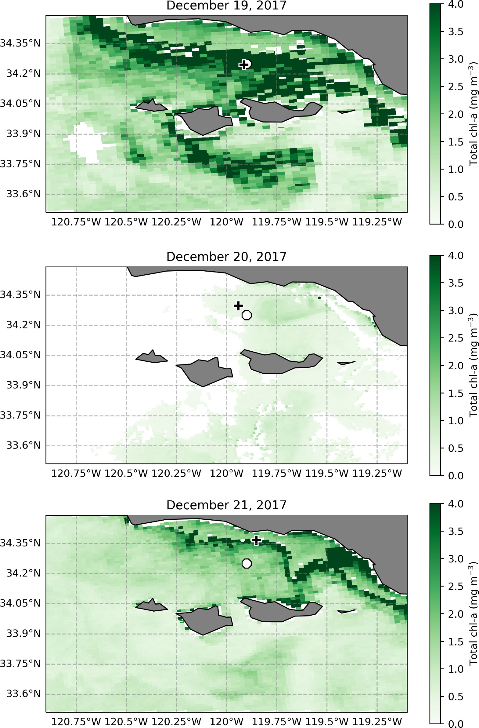
Figure 1 MODIS chlorophyll-a concentration for December 19, December 20, and December 21, 2017. The location of in situ sampling for each day is shown as a black cross. The location of Plumes and Blooms Station 4 is shown in a white octagon. White patches on December 19 and 20 were masked out and flagged due to cloud cover, high polarization, or other product failures.

2.2 In situ measurements

2.2.1 Compact-Optical Profiling System (C-OPS) reflectance

The Compact-Optical Profiling System (C-OPS, Biospherical Instruments, Inc.) was used to measure upwelling spectral radiance ($L_u(\lambda )$) and downwelling spectral irradiance ($E_d(\lambda )$) from 320 and 780 nm at 18 distinct wavelengths. Instrument deployment and data processing for the C-OPS in free-fall mode followed methods presented in Toole and Siegel (2001); Kostadinov et al. (2007); Barrón et al. (2014), and Henderikx Freitas et al. (2017). The instrument was deployed at noon from the stern of the ship to minimize the influence of ship shadow or solar zenith angle on the measurements. Remote sensing reflectance just below the surface, $r_{rs}(\lambda )$, was obtained following equation 4 (Mobley, 1994):

$\begin{array}{ll}{r}_{rs}(\lambda )= \frac{L_u(\lambda )}{E_d(\lambda )}.& \text{[4]}\end{array}$

$r_{rs}(\lambda )$ was then converted to remote sensing reflectance just above the surface of the water, $R_{rs}(\lambda )$, following Lee et al. (2002):

$\begin{array}{ll}{R}_{rs}(\lambda )=\frac{0.52* r_{rs}(\lambda )}{1-1.7*r_{rs}(\lambda )}.& \text{[5]}\end{array}$

C-OPS samples were collected from December 17-21, 2017 (Supplementary Figure 1A). Replicate profiles were obtained to produce uncertainty estimates (Figure 2A).

FIGURE 2

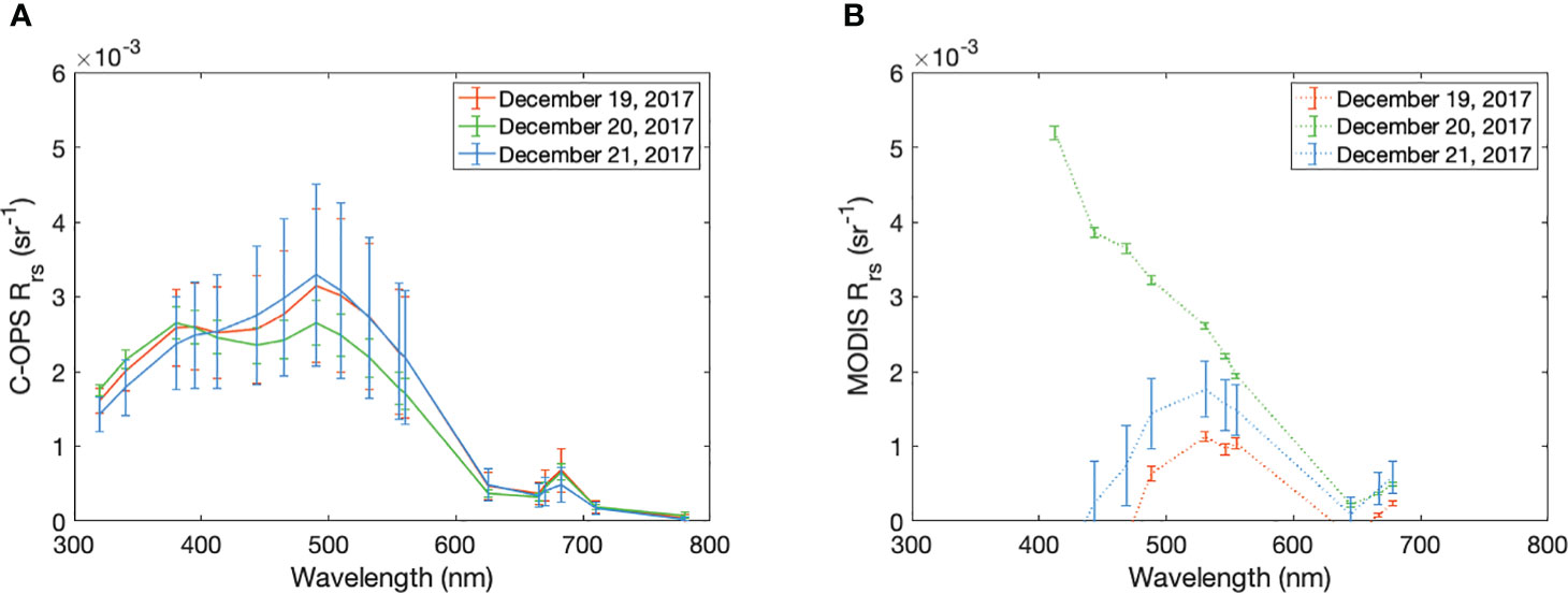
Figure 2 Remote sensing reflectance measured (A) in situ with the C-OPS and (B) from space with MODIS. Spectra were measured on December 19 (red), December 20 (green), and December 21 (blue), 2017. Error bars show +/- 1 standard deviation: for C-OPS, within the top 1m of water; for MODIS-Aqua, within the 5x5 pixel box surrounding the C-OPS cast site.

2.2.2 Filter pad absorption by phytoplankton (${\mathrm{aph}}_{}$(λ)) and non-algal particles ($a_d$(λ))

Two-liter whole seawater samples (N = 24) were collected from the surface (<5 m) Niskin bottle from the CTD rosette and filtered through 0.7µm 25 mm GF/F filters (Whatman), which were then folded in half and stored in pre-labeled aluminum foil packets. Filters were stored immediately in liquid nitrogen for 1 week and at -80°C for 5 months until analysis. Three blank samples were prepared at sea by filtering 2L MilliQ water through the same filter type at the same pump pressure and were stored in the same way as the discrete samples until the time of analysis. Just before analysis, one laboratory blank was prepared by filtering 2L MilliQ water. This sample was used as the reference blank in the spectrophotometer.

A Shimadzu UV-2401PB dual-beam spectrophotometer with a 60 mm diameter ISR-2200 integrating sphere was used to measure optical densities of particulate material on the filter, $O{D}_f(\lambda )$. Samples were run in transmission-reflectance (T-R) mode. Frozen samples were thawed prior to analysis. Filters were kept hydrated and protected from light when not in the spectrophotometer. Samples were placed on the integrating sphere and run against the laboratory blank reference filter. All filters were scanned first for total particulate absorption ($a_p(\lambda )$). The filters were then extracted in methanol (following Kishino et al., 1985): 10ml hot methanol was poured carefully on each filter and allowed to sit for a few minutes before filtering through. The hot methanol rinse was repeated, and each filter was then rinsed with ~20ml boiling MilliQ water to remove phycobiliproteins, which do not extract in methanol (Roesler et al., 2018). Filters were then re-scanned for non-algal (depigmented) particle absorption ($a_d(\lambda )$). All samples and blanks were scanned 3 times (with a 90° rotation between each scan) to obtain an average scan for all measured blanks and samples. The averaged blank filter absorbance was subtracted from the averaged absorbance of the corresponding sample filter. All spectra were zeroed at 850 nm as needed, where no absorbance is expected, following the beta-correction approach of Roesler (1998).

Absorbance was converted to absorption and all spectra were corrected for pathlength amplification following the recommendations of the IOCCG protocols (Roesler et al., 2018) based on Tassan and Ferrari (1995) and Stramski et al. (2015) for a spectrophotometer in transmittance-reflectance (T-R) mode with an integrating sphere and externally-mounted samples, where the optical density of particulate material on the filter ($O{D}_f(\lambda )$) is corrected to absorbance, $O{D}_s(\lambda )$, following equation 6:

$\begin{array}{ll}O{D}_s(\lambda )=0.719{(O{D}_f(\lambda ))}^{1.2287}.& \text{[6]}\end{array}$

Absorbance ($O{D}_s(\lambda )$) is then converted to absorption ($a_p(\lambda )$) following equation 7:

$\begin{array}{ll}{a}_p(\lambda )=\frac{2.303}{pathlength}* O{D}_s(\lambda )& \text{[7]}\end{array}$

where the pathlength is the volume filtered (m³) divided by the area of the filter (m²), which was measured for each sample. This correction was applied to all particulate and depigmented particle absorption spectra. Finally, spectral absorption by phytoplankton ($a_{ph}(\lambda )$) is computed as the difference between total particulate absorption ($a_p(\lambda )$) and depigmented particulate ($a_d(\lambda )$) absorption coefficients.

2.2.3 Colored dissolved organic matter (CDOM) absorption ($a_g$(λ))

CDOM absorption ($a_{ɡ}(\lambda )$) was measured following Nelson et al. (2007). Whole seawater samples (N = 21) were collected from the surface Niskin bottle in 100ml amber glass vials. Samples were filtered immediately at sea using pre-extracted 0.2µm polycarbonate filters (Nuclepore). The filtrate was collected in amber glass EPA vials and kept in the dark at 4°C until analysis. Samples were equilibrated to room temperature before analysis. CDOM absorption ($a_{ɡ}(\lambda )$) was measured using an UltraPath single beam spectrophotometer (World Precision Instruments). Optical density ($O{D}_s(\lambda )$) was measured and adjusted to $a_{ɡ}(\lambda )$ following equation 7, where the pathlength was 0.1m. Salinity corrections were applied as in Nelson et al. (2007).

2.2.4 High Performance Liquid Chromatography (HPLC) pigments

Two-liter whole seawater samples were collected from the surface Niskin bottle. Samples were filtered through 0.7µm 25 mm Whatman GF/F filters and stored immediately in liquid nitrogen until analysis at NASA’s Goddard Space Flight Center (GSFC) by the Ocean Biology Processing Group following Van Heukelem and Thomas (2001) and Van Heukelem and Hooker (2011). Total chlorophyll-a (Tchla; the sum of monovinyl chlorophyll-a, divinyl chlorophyll a, chlorophyllide, and chlorophyll-a allomers and epimers) from HPLC was used here to compare to ocean color estimates (24 samples total were collected; 3 samples are shown here for comparison with exact matchups with ocean color data).

2.3 Generalized IOP algorithm (GIOP) applied to in situ$R_{rs}$(λ)

The Generalized IOP (GIOP) algorithm of Werdell et al. (2013) was used to invert in situ $R_{rs}(\lambda )$ measured with the C-OPS to retrieve spectral inherent optical properties. With the input of $R_{rs}(\lambda )$, GIOP uses the OC4 algorithm to estimate chlorophyll concentration (https://oceancolor.gsfc.nasa.gov/atbd/chlor_a/) and model particle backscattering ($b_{bp,mod}(\lambda )$), total absorption by CDOM and particles ($a_{pɡ,mod}(\lambda )$), absorption by phytoplankton ($a_{ph, mod}(\lambda )$), and absorption by CDOM and depigmented particles ($a_{dɡ,mod}(\lambda )$). Since the GIOP in the default configuration was developed for the open ocean and the Santa Barbara Channel is a coastal site, the slope of $a_{dɡ}(\lambda )$ was adjusted from the default value of 0.018 to 0.012 to reflect the higher values typically found in coastal regions (Roesler et al., 1989) and compare the resulting model performance vs. in situ IOP data. All other parameters were used at their default values. While the GIOP is typically applied to satellite data, in our study, the GIOP was only applied to the C-OPS $R_{rs}(\lambda )$ spectra. Satellite $R_{rs}(\lambda )$ data could not be inverted due to failures in the GIOP given the data quality.

2.4 MODIS-Aqua Level 2 1-km products

MODIS-Aqua Level 2 1-km remote sensing reflectance products were downloaded from the NASA Ocean Biology Processing Group (https://oceancolor.gsfc.nasa.gov). The most recent reprocessing (R2022) was used. While there were MODIS-Aqua images for each day of in situ sampling, there were only concurrent images of the location where C-OPS, inherent optical properties (IOPs), and HPLC samples were collected on December 19-21, 2017. Following the matchup criteria presented by Bailey and Werdell (2006), $R_{rs}(\lambda )$ values were averaged for the 5x5 pixel box around the in situ observations. While many pixels in the match-up region were flagged due to high polarization or other product failures, no pixels contained any of the exclusion flags specified by Bailey and Werdell (2006). It is of particular note that no spectra were flagged for a failed atmospheric correction algorithm (given by the ATMFAIL flag) and the product failures related to failed derived products (i.e., particulate inorganic carbon; PIC) rather than any other common flags (Sean Bailey, pers. comm.). However, the coefficient of variation was greater than 0.15 for multiple wavelengths of the December 19 and December 21 spectra, meaning that only the December 20 spectrum passed all Bailey and Werdell (2006) criteria. The spectra provide relevant context for the in situ samples and highlight the challenges of relying on ocean color when atmospheric interference is higher (e.g., during a coastal wildfire). In addition to $R_{rs}(\lambda )$ spectra, we also retrieved the standard mass concentration of chlorophyll-a provided in the Level-2 data files (details at https://oceancolor.gsfc.nasa.gov/atbd/chlor_a/). Chlorophyll-a from MODIS Aqua compares favorably to in situ measurements in this region (Siegel et al., 2003; Li et al., 2008; Anderson et al., 2008).

2.5 Plumes and Blooms sampling

Optical data from winter monthly cruises (defined as November to January) collected through the Plumes and Blooms sampling program (PnB; http://www.oceancolor.ucsb.edu/plumes_and_blooms/) were used to compare the historical context of the Santa Barbara Channel during years without wildfires. Plumes and Blooms has monitored the bio-optical variability of the Santa Barbara Channel along a consistent, 7-station transect approximately monthly since 1996. Samples were collected for $a_d(\lambda )$, $a_{ph}(\lambda )$, and $a_{ɡ}(\lambda )$ using the same methods detailed above. Only surface data from Station 4 (34’15.01°N, 119’54.38°W) were used for this comparison, as it was collocated with the sampling locations use throughout the Thomas Fire cruise. A total of 28 samples, collected in winter cruises between 2005-2016 and in 2018, were used here.

3 Results

The impact of wildfire smoke and ash on reflectance as measured by the C-OPS in situ was compared to reflectance measured by MODIS-Aqua via remote sensing. The shape and magnitude of C-OPS $R_{rs}(\lambda )$ spectra were relatively consistent between the three days of sampling (Figure 2A). Relatively lower $R_{rs}(\lambda )$ values in the blue wavelengths (350-450nm) suggest high absorption by CDOM and NAP. A chlorophyll fluorescence peak is present at 670nm, consistent with the relatively high chlorophyll-a concentrations measured from HPLC on these days (Figure 3C). Alternately, the shape and magnitude of $R_{rs}(\lambda )$ spectra measured from MODIS-Aqua are quite different across the three days of sampling and do not match the C-OPS spectra measured on those same days and times (Figure 2B).

FIGURE 3

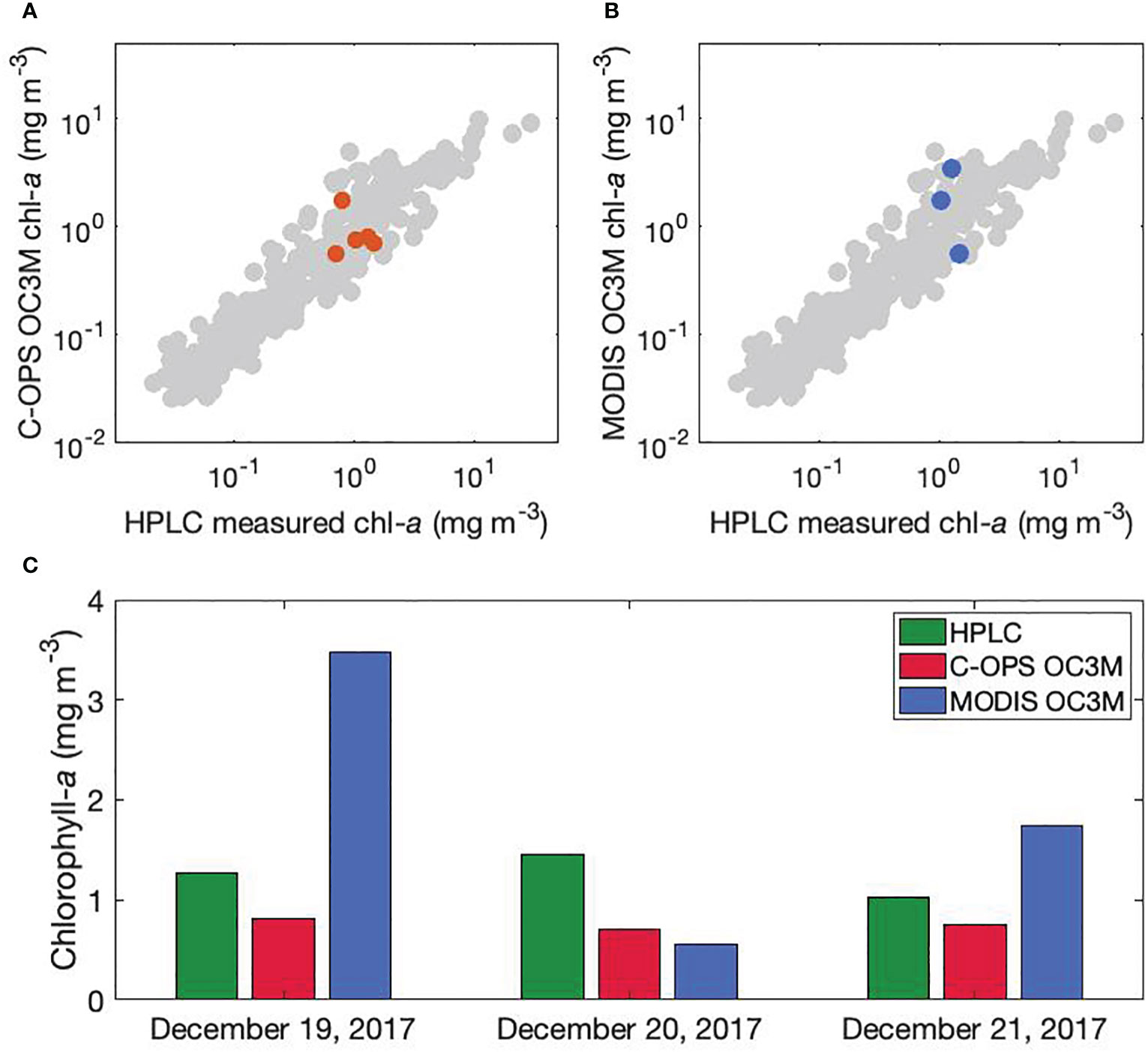
Figure 3 Chlorophyll-a concentration calculated using the OC3M algorithm (NASA GSFC; https://oceancolor.gsfc.nasa.gov/atbd/chlor_a/) for (A) C-OPS samples and (B) MODIS-Aqua samples, both overlaid on the NOMAD dataset for context (Werdell and Bailey, 2005). Chlorophyll-a concentrations from the three match-up days are compared in (C) to concentrations measured by HPLC.

The discrepancies between satellite and in situ ocean color spectra necessarily result in different chlorophyll-a retrievals from the OC3M algorithm, which uses a ratio between the blue and green wavelengths to calculate chlorophyll-a concentration. The MODIS-Aqua spectra are theoretically unrealistic, in that these spectral shapes do not reflect realistic scenarios for radiative transfer in the ocean. When the derived chlorophyll-a concentrations from these satellite and in situ $R_{rs}(\lambda )$ spectra are compared directly to each other and to chlorophyll-a measured from HPLC, chlorophyll-a from MODIS-Aqua exceeds chlorophyll-a from C-OPS and HPLC by a factor of 3 on December 19 and by a factor of 2 on December 21 (Figure 3C). On December 20, MODIS-Aqua chlorophyll-a is lower than HPLC and C-OPS chlorophyll-a. In all cases, the MODIS-Aqua chlorophyll-a estimates demonstrate the poorest relationship with HPLC chlorophyll-a or chlorophyll-a from C-OPS. The chlorophyll-a concentrations retrieved from C-OPS reflectances (Figure 3A) and MODIS-Aqua reflectances (Figure 3B) are within normal ranges, particularly when compared to the range of samples included in the NASA bio-Optical Marine Algorithm Dataset (NOMAD). However, the MODIS-Aqua values are on the outer limits of the relationship between observed between modeled and measured chlorophyll-a concentrations in the NOMAD dataset.

The bio-optical context in which these samples were collected is considered more holistically via the direct measurement of inherent optical properties (IOPs). Comparing the average $a_{ph}(\lambda )$, $a_{ɡ}(\lambda )$, and $a_d(\lambda )$ coefficients during the Thomas Fire (Figure 4A) to the mean values of these properties during a typical December (2005-2018) in the Santa Barbara Channel from PnB highlights the differences during the Thomas Fire (Figure 4B). Non-algal particulate absorption and CDOM absorption had similar magnitudes in December 2017 to historical Decembers, but phytoplankton absorption was relatively lower in December 2017. Accordingly, the $a_{ɡ}(\lambda )$ to $a_{ph}(\lambda )$ ratio and $a_d(\lambda )$ to $a_{ph}(\lambda )$ ratio were much higher during the Thomas Fire than is expected in the Santa Barbara Channel in December (Figure 4C). The absorption budgets demonstrate that $a_{ɡ}(\lambda )$ dominated the overall absorption in the blue and green wavelengths in December 2017 compared to the relatively high phytoplankton absorption signal relative to other absorbing components in a typical December (Figure 4D).

FIGURE 4

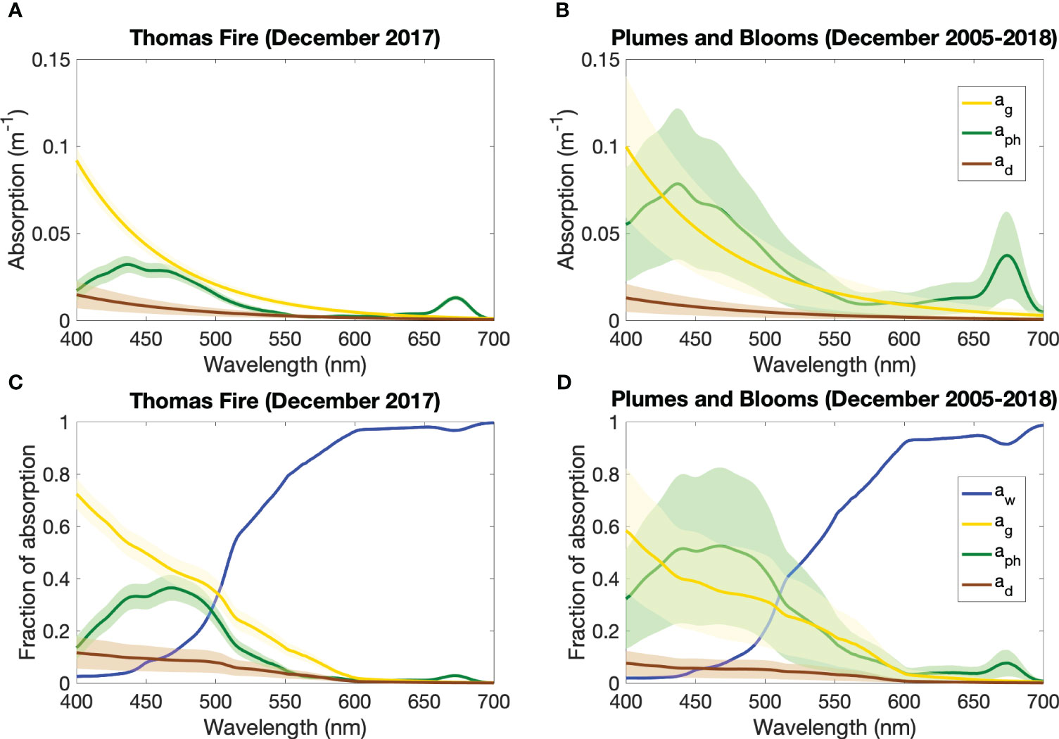
Figure 4 Mean absorption by CDOM ($a_g(\lambda )$, yellow), phytoplankton ($a_{ph}(\lambda )$, green), and non-algal particles ($a_d(\lambda )$, brown) from (A) December 2017 and (B) other Decembers in the Plumes and Blooms dataset. Shading shows +/- one standard deviation of the mean value at each wavelength. The fractional contribution of each component to total absorption at each wavelength for these datasets is shown in (C) for December 2017 and (D) for other Decembers from Plumes and Blooms Station 4. Pure seawater absorption is also shown (Pope and Fry, 1997).

Finally, the reflectance and IOP data were combined to consider the effects of wildfire smoke and ash on optical modeling. The measured IOP spectra were compared to the modeled IOP spectra from the inversion of C-OPS data measured in situ. GIOP retrieved the magnitude and relative shape of the mean $a_{ph}(\lambda )$ spectra with high accuracy (Figure 5A), but underestimated the magnitude of CDOM+NAP absorption ($a_{dɡ,mod}(\lambda )$; Figure 5B), resulting in an underestimation of the total summed particulate absorption term ($a_{pɡ,mod}(\lambda )$; Figure 5C). When the slope of $a_{dɡ}(\lambda )$ was adjusted to reflect the conditions expected in coastal regions (Supplementary Figure 2; Roesler et al., 1989; Werdell et al., 2013), the mean $a_{pɡ,mod}(\lambda )$ spectra are the same magnitude as the mean measured $a_{pɡ}(\lambda )$ spectra at most wavelengths (Supplementary Figure 2C), but the magnitude of $a_{ph}(\lambda )$ was underestimated relative to measured values (Supplementary Figure 2A).

FIGURE 5

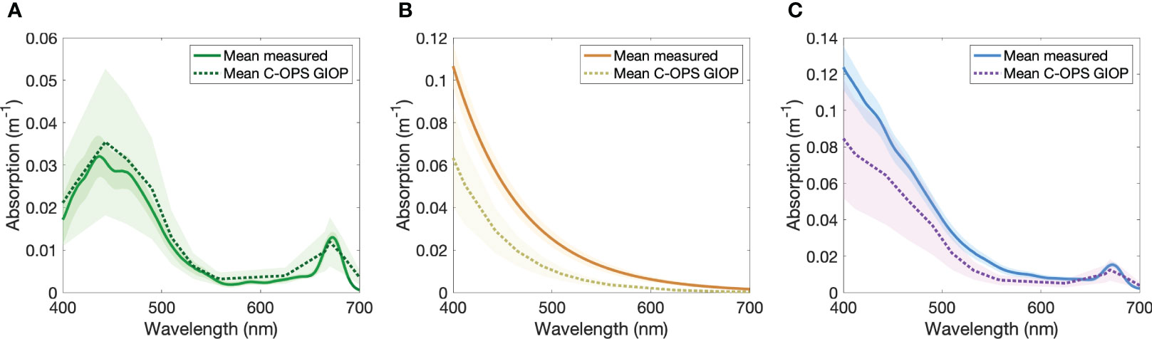
Figure 5 Mean measured (solid lines) and modeled (dashed lines) inherent optical properties. (A) Phytoplankton absorption ($a_{ph}(\lambda )$), (B) summed CDOM and depigmented particulate absorption ($a_{dg}(\lambda )$), and (C) total particulate and CDOM absorption ($a_{pg}(\lambda )$). Shading shows +/- one standard deviation of the mean value at each wavelength.

4 Discussion

Our study leverages satellite data, in situ data, and time series data to explore the impacts of wildfires on ocean properties, including the potential effects of smoke, ash particle deposition, and increased dissolved organic matter from ash leachate. Of these three data sources, the satellite data were the easiest and cheapest data to collect. However, for our study region during this sampling period, these data were not of sufficient quality to evaluate ocean color or derived products. The variability in the MODIS-Aqua $R_{rs}(\lambda )$ spectra, which were measured from the top of atmosphere to capture ocean color just above the surface of the water, are consistent with the variable smoke coverage over the sampling site on each day of sampling (Figure 2B; Kramer et al., 2020). These spectra result in excessively high (December 19, 21) or low (December 20) chlorophyll-a concentrations compared to HPLC (Figure 3C). The MODIS-Aqua $R_{rs}(\lambda )$ spectra show three different but theoretically unrealistic spectral shapes compared to the consistent measurements of $R_{rs}(\lambda )$ from the C-OPS (Figure 2). Only the spectra measured on December 20 passed the Bailey and Werdell (2006) quality control assessment for validation-quality ocean color data, and none of these spectra were suitable for inversion using GIOP. Furthermore, these spectra were only flagged due to high polarization. More specifically, none of the flags masked in Level 3 data were triggered, meaning that these pixels would have been included in the generation of Level 3 data products. As Level 3 data are generally used for ocean color applications, these pixels could potentially be used to assess the impact of wildfires on marine ecosystems, despite clear data quality issues.

The difficulty of retrieving accurate chlorophyll concentrations from remote sensing methods has been observed in other optically-complex marine systems with impacts of dust, atmospheric aerosols, or high CDOM concentrations (Claustre et al., 2002; Stramska et al., 2008; Lewis and Arrigo, 2020 and references therein). While these exact effects have not been observed in situ for coastal wildfire conditions prior to this study, our results are consistent with the optical properties of other ecosystems influenced by absorbing constituents in the atmosphere and/or ocean. In assessing the impact of the wildfire smoke and ash on the quality of the satellite $R_{rs}(\lambda )$ data, documented challenges with atmospheric correction of $R_{rs}(\lambda )$ data over the Santa Barbara Channel were also considered (e.g., Henderikx Freitas et al., 2017). When the spectra were assessed with the Quality Water Index Polynomial (QWIP; Dierssen et al., 2022), the remote sensing data collected over the Santa Barbara Channel in December 2017 during the Thomas Fire had a QWIP score that was comparable to the MODIS-Aqua timeseries over the same region in Decembers 2002-2022 (Supplementary Figure 3), suggesting that there was still the average amount of usable data collected in this region during the Thomas Fire as in wildfire-free years. Other aerosol sources may also contribute to poor atmospheric correction for remote sensing data. In this case study, the role of marine aerosol-producing phytoplankton (e.g., dimethylsulfide producers) can be ruled out following a high-resolution characterization of the phytoplankton community during this period (Kramer et al., 2020). Ultimately, given the quality of the satellite $R_{rs}(\lambda )$ data, these data were not useful for evaluating the color of the ocean or the potential ecological impact of the wildfire on the ocean.

In this study, we were fortunate to have a serendipitous research cruise already planned in the region where the fire broke out (Bisson et al., 2020). The in situ samples collected alongside in situ ocean color measurements in this study provide important points of comparison and more detailed information about the bio-optical regime of the Santa Barbara Channel during the Thomas Fire. The in situ reflectance data demonstrate the impact of the Thomas Fire on the coastal ocean. The C-OPS $R_{rs}(\lambda )$ spectra, which were measured below the wildfire smoke plume and just below the surface of the water, are consistent in shape and magnitude, resulting in more accurate chlorophyll-a retrievals relative to HPLC (Figure 3C). These spectra were not impacted by the same quality control concerns as the satellite ocean color data, and were more suitable for both direct analysis (Figure 2A) and inversion approaches (Figure 5). While the short length of this cruise resulted in relatively few direct matchups between in-water $R_{rs}(\lambda )$ and satellite $R_{rs}(\lambda )$, we collected surface in-water optical samples in duplicate or triplicate, leading to a larger dataset against which to compare the satellite samples (21-24 samples, depending on the variable).

The in situ IOP data collected alongside the reflectance data help to further demonstrate some of the variability in different oceanic components during the Thomas Fire compared to a typical December in the Santa Barbara Channel. When the in situ absorption spectra are compared to the absorption by different optically significant components estimated by inversion modeling, the strengths and weaknesses of that type of ocean color model can be considered in a coastal ecosystem undergoing an extreme ecological event, such as during the Thomas Fire. The results shown here demonstrate that inversion models may capture some components of the reflectance signal ($a_{ph}(\lambda )$, Figure 5A) better than others ($a_{dɡ}(\lambda )$ and $a_{pɡ}(\lambda )$, Figures 5B, C). GIOP solves for $R_{rs}(\lambda )$ as a balance of absorption to backscattering (Equations 1-3). In this system, the unexpectedly high in situ $a_{ɡ}(\lambda )$ signal during the Thomas Fire relative to other absorbing constituents (Figure 4C) was not retrieved by inversion modeling using the GIOP in its default configuration. When a higher $a_{dɡ}(\lambda )$ slope was applied, the shape and magnitude of the $a_{dɡ,mod}(\lambda )$ spectra and $a_{pɡ,mod}(\lambda )$ spectra were a better fit to the measured data (Supplementary Figure 2B, C). However, the $a_{ph,mod}(\lambda )$ spectra underestimated the magnitude of the measured $a_{ph}(\lambda )$ data (Figure 2A), demonstrating the difficulty of capturing absorption by all optical components in a complex region with high concentrations of phytoplankton and other absorption constituents, such as the coastal ocean during a wildfire.

Finally, the PnB time series was leveraged to put the optical and pigment data in a broader historical and ecological context. In Kramer et al. (2020), the PnB pigment data contextualized the abundance and magnitude of different phytoplankton groups during the Thomas Fire relative to a typical December. In this work, the in situ IOP data from PnB was compared to the data collected during the fire. The relatively low phytoplankton absorption coefficient in December 2017 (Figures 4A, B) was expected given the lower chlorophyll-a concentrations measured in December 2017 compared to the PnB average (Kramer et al., 2020), and the magnitude of the measured $a_{ph}(\lambda )$ in December 2017 matches the values retrieved from in situ ocean color inversion during this same period (Figure 5A). The relatively high $a_{ɡ}(\lambda )$ coefficient during the Thomas Fire compared to other IOPs (Figures 4C, D) is consistent with recent studies showing increased deposition of black carbon and dissolved organic matter from wildfires to the coastal ocean (Wagner et al., 2021; Coward et al., 2022). Despite the relatively high chlorophyll-a concentrations during the Thomas Fire, the optical signal was not dominated by phytoplankton, but rather by CDOM absorption.

While satellite data are the cheapest and most readily-available form of data to leverage during an extreme event such as the Thomas Fire, for our study region and during this wildfire, these data did not have sufficient quality to allow evaluation of ocean color. Instead, in situ measurements of $R_{rs}(\lambda )$, IOPs, and chlorophyll-a allowed for a system-wide evaluation of the conditions in the SBC during the Thomas Fire. The in situ optical and pigment data from the PnB time series also contextualized these results within the broader context of the region and ecosystem. In many recent studies examining wildfire impacts on the ocean, particularly in more remote or open ocean environments, in situ samples are not available (Ardyna et al., 2022; Wang et al., 2022; Weis et al., 2022). Inversion modeling and derived products are essential in these cases: all three studies used chlorophyll-a from remote sensing to consider the possibility of a phytoplankton bloom occurring in the wake of a wildfire smoke plume. The relationship between $b_{bp}(\lambda )$ and phytoplankton carbon ($C_{phyto}$) was also used to further describe the impact of wildfires on primary productivity beyond the chlorophyll-a concentration (i.e., photoacclimation, physiological stress; Wang et al., 2022; Weis et al., 2022). The accuracy of these two parameters (chlorophyll, $C_{phyto}$) is paramount to the interpretation of results and significance. The results shown here demonstrate that the derivation of these parameters is certainly also impacted by the wildfire, particularly from remote sensing. In situ sampling of IOPs and reflectance highlights an optical signature of the wildfire, but the accuracy of these measurements was only made possible by shipboard collection below the smoke plume, and the anomaly of these results was only made clear by comparison to time series data.

While ocean color has been and will remain an important, economical tool for considering the effects of wildfires on marine ecosystems, more high-quality measurements of IOPs and reflectance in situ during wildfires are urgently needed. As remote sensing approaches gain popularity for monitoring and evaluating the impacts of wildfires on the coastal and open ocean, it is essential to compare the performance of these approaches with in situ measurements in different ecosystems and regions. The impacts of wildfires on the ocean may often be nonlinear (e.g., wildfire smoke may block available light for photosynthesis, while leaching ash may provide limiting nutrients). It is important to have in-water measurements to evaluate these impacts in near real-time, particularly to compare to daily or weekly satellite measurements. Our results demonstrate that the impacts of wildfires on ocean ecology and optics may also vary based on the proximity to the wildfire. In the coastal ocean, increased CDOM from ash leaching may impact both ocean color (as seen in the shape and magnitude of the in situ C-OPS $R_{rs}(\lambda )$ spectra; Figure 2A) and in situ IOPs (Figures 5B, C; Supplementary Figures 2B, C). In situ measurements will also allow for an evaluation of the impact of these other optically significant materials on the estimation of chlorophyll-a from remote sensing, particularly if further conclusions about ecosystem impacts will be drawn from an enhanced chlorophyll signal (e.g., Ardyna et al., 2022; Wang et al., 2022; Weis et al., 2022).

Finally, this study has demonstrated the ongoing challenge of “known unknowns” in work at the intersection of unpredictable extreme events (e.g., wildfires, volcanic eruptions) and ocean ecosystems (Bisson et al., in revision). While many elements of the system can be described or directly quantified (such as chlorophyll-a concentrations, absorption coefficients, reflectance spectra), there are many unknowns that cannot always be captured or investigated on the appropriate timescale—the thickness of the smoke plume throughout the day, the amount of ash deposition and variability in ash composition, the rate of ash dissolution in natural seawater compared to laboratory studies, the retentiveness of the physical environment, etc. The combination of the dynamic ocean system and the unpredictable, ever-changing landscape of a wildfire may not be possible to capture in full detail, but the combination of remote sensing observations and in situ validation studies will ideally help to constrain the (near) real-time impacts of the fire on the ocean. As wildfires continue to increase in size and severity, particularly in coastal regions, future studies to quantify these impacts will be essential. Furthermore, the advent of satellite sensors with higher spectral resolution (e.g., NASA’s Plankton Aerosol Cloud and ocean Ecosystem [PACE] sensor; Werdell et al., 2019) will allow for more information to be gathered from remote sensing during coastal wildfires, such as measurements of phytoplankton pigment concentrations that can link to community composition (Kramer et al., 2022). With these higher-resolution measurements and derived products, quality control and in situ samples for validation will remain essential, particularly during significant ecological disturbances.

5 Conclusions and recommendations

We close with three concrete recommendations for wildfire-ocean work going forward, based on the lessons learned and results shown here.

1) Coastal timeseries are essential for continuing observations and to provide historical context during a wildfire or other extreme event/ecological disturbance. In this study, the PnB dataset was compared to the higher-resolution sampling during the Thomas Fire to consider those results in the context of a typical December in the Santa Barbara Channel. As much as possible, we encourage the integration of optical measurements to these coastal time series, which are critical for remote sensing validation. Both reflectance and IOP measurements will help to confirm the patterns shown in ocean color observations and constrain the outcome of derived products.

2) Planning field work to collect in situ samples around an unpredictable event such as a wildfire may not be possible, and thus remote sensing will remain a vital tool for monitoring; however, whenever possible, we strongly recommend the collection of in situ samples to validate and confirm the results of these remote sensing measurements. Sample collection is more difficult in open ocean regions, but other autonomous resources beneath the smoke plume can be used in these cases when possible (e.g., floats, buoys, AERONET sensors, etc.).

3) We encourage funding agencies to develop creative opportunities for providing money and resources quickly when wildfires occur in coastal regions or when wildfire impacts in open ocean regions are observed from remote sensing (similar to the RAPID model, but ideally providing resources on timescales of days to weeks within the realistic course of most wildfires). Contingency plans should be in place for use of existing research vessels or smaller ships during wildfires or other extreme events, and where possible, funding should be set aside to mobilize for sample collection and analysis during these times. While these unpredictable events provide a logistical and financial challenge, more research is clearly needed in this area. The extremely limited datasets presented in existing in situ studies are likely only representative of those regions at that one moment in time, and a more holistic understanding of the impacts of wildfires on marine systems can only be reached with an investment of time, resources, and creative thinking.

Data availability statement

The datasets presented in this study can be found in online repositories. The names of the repository/repositories and accession number(s) can be found below: https://seabass.gsfc.nasa.gov/cruise/ACIDD_2017, https://seabass.gsfc.nasa.gov/experiment/Plumes_and_Blooms, https://www.earthdata.nasa.gov/eosdis/daacs/obdaac.

Author contributions

SK: Conceptualization, Data curation, Formal Analysis, Investigation, Methodology, Project administration, Visualization, Writing – original draft, Writing – review & editing. KB: Conceptualization, Data curation, Formal Analysis, Funding acquisition, Investigation, Methodology, Project administration, Writing – review & editing. CM: Conceptualization, Data curation, Formal Analysis, Funding acquisition, Investigation, Methodology, Project administration, Visualization, Writing – review & editing.

Funding

The author(s) declare financial support was received for the research, authorship, and/or publication of this article. The University of California’s Ship Funds Program, the National Academies Keck Futures Initiative, UCSB’s Coastal Fund, NASA grant #NNX17AK04G to Kyla Drushka, and NSF grant #1821916 to David Valentine provided funding for this project. The Plumes and Blooms time series is supported by NASA Ocean Biology and Biogeochemistry. SK is supported by NASA grant #80NSSC21K0015 to Colleen A. Durkin, the David and Lucille Packard Foundation, and a Simons Foundation Postdoctoral Fellowship in Marine Microbial Ecology. CM is supported by NPRB grant #2101A to CM. Funding for publication comes from NASA TWSC grant #80NSSC22K0049 to KB.

Acknowledgments

This work could not have been accomplished without the enthusiastic support of the Captain and crew of R/V Sally Ride and all other members of the ACIDD science team. Thank you to Crystal Thomas at NASA GSFC for processing the ACIDD and PnB HPLC samples with high precision and accuracy. Thank you also to Paula Bontempi, Laura Lorenzoni, and Ivona Cetinić for support with HPLC sample processing. Collin Roesler and Aimee Neeley provided helpful comments on the phytoplankton absorption data. Jeremy Werdell, Amir Ibrahim, and Sean Bailey provided important context for the remote sensing data. Thank you to Nathalie Guillocheau and Dylan Catlett for PnB sample help. We are grateful for support from Dave Siegel. Comments from Robert Frouin and four reviewers helped to improve earlier versions of this manuscript.

Conflict of interest

The authors declare that the research was conducted in the absence of any commercial or financial relationships that could be construed as a potential conflict of interest.

Publisher’s note

All claims expressed in this article are solely those of the authors and do not necessarily represent those of their affiliated organizations, or those of the publisher, the editors and the reviewers. Any product that may be evaluated in this article, or claim that may be made by its manufacturer, is not guaranteed or endorsed by the publisher.

Supplementary material

The Supplementary Material for this article can be found online at: https://www.frontiersin.org/articles/10.3389/fmars.2023.1267681/full#supplementary-material

References

Abram N. J., Gagan M. K., McCulloch M. T., Chappell J., Hantoro W. S. (2003). Coral reef death during the 1997 Indian Ocean dipole linked to Indonesian wildfires. Science 301 (5635), 952–955. doi: 10.1126/science.1083841

PubMed Abstract | CrossRef Full Text | Google Scholar

Anderson C. R., Siegel D. A., Kudela R. M., Brzezinski M. A. (2008). Empirical models of toxigenic Pseudo-nitzschia blooms: Potential use as a remote detection tool in the Santa Barbara Channel. Harmful. Algae. 8 (3), 478–492. doi: 10.1016/j.hal.2008.10.005

CrossRef Full Text | Google Scholar

Ardyna M., Hamilton D. S., Harmel T., Lacour L., Bernstein D. N., Laliberté J., et al. (2022). Wildfire aerosol deposition likely amplified a summertime Arctic phytoplankton bloom. Commun. Earth Environ. 3 (1), 201. doi: 10.1038/s43247-022-00511-9

CrossRef Full Text | Google Scholar

Bailey S. W., Werdell P. J. (2006). A multi-sensor approach for the on-orbit validation of ocean color satellite data products. Remote Sens. Environ. 102, 12–23. doi: 10.1016/j.rse.2006.01.015

CrossRef Full Text | Google Scholar

Barrón R. K., Siegel D. A., Guillocheau N. (2014). Evaluating the importance of phytoplankton community structure to the optical properties of the Santa Barbara Channel, California. Limnol. Oceanogr. 59 (3), 927–946. doi: 10.4319/lo.2014.59.3.0927

CrossRef Full Text | Google Scholar

Bisson K. M., Baetge N., Kramer S. J., Catlett D., Girling G., McNair H., et al. (2020). California wildfire burns boundaries between science and art. Oceanography 33 (1), 16–19. doi: 10.5670/oceanog.2020.110

CrossRef Full Text | Google Scholar

Bisson K. M., Boss E., Werdell P. J., Ibrahim A., Frouin R., Behrenfeld M. J. (2021). Seasonal bias in global ocean color observations. Appl. Optics. 60 (23), 6978–6988. doi: 10.1364/AO.426137

CrossRef Full Text | Google Scholar

Bisson K. M., Gassó S., Mahowald N., Wagner S., Koffman B., Carn S. A., et al. (2023). Observing ocean ecosystem responses to volcanic ash. Remote Sens. Environ. 296, 1–13. doi: 10.1016/j.rse.2023.113749

CrossRef Full Text | Google Scholar

Browning T. J., Stone K., Bouman H. A., Mather T. A., Pyle D. M., Moore C. M., et al. (2015). Volcanic ash supply to the surface ocean—remote sensing of biological responses and their wider biogeochemical significance. Front. Mar. Sci. 2. doi: 10.3389/fmars.2015.00014

CrossRef Full Text | Google Scholar

Cira M., Bafna A., Lee C. M., Kong Y., Holt B., Ginger L., et al. (2022). Turbidity and fecal indicator bacteria in recreational marine waters increase following the 2018 Woolsey Fire. Sci. Rep. 12 (1), 2428. doi: 10.1038/s41598-022-05945-x

PubMed Abstract | CrossRef Full Text | Google Scholar

Claustre H., Morel A., Hooker S. B., Babin M., Antoine D., Oubelkheir K., et al. (2002). Is desert dust making oligotrophic waters greener? Geophys. Res. Lett. 29 (10), 107–101. doi: 10.1029/2001GL014056

CrossRef Full Text | Google Scholar

Coombs J. S., Melack J. M. (2013). Initial impacts of a wildfire on hydrology and suspended sediment and nutrient export in California chaparral watersheds. Hydrol. Processes. 27, 3842–3851. doi: 10.1002/hyp.9508

CrossRef Full Text | Google Scholar

Coward E. K., Seech K., Carter M. L., Flick R. E., Grassian V. H. (2022). Of sea and smoke: evidence of marine dissolved organic matter deposition from 2020 western United States wildfires. Environ. Sci. Technol. Lett. 9 (10), 869–876. doi: 10.1021/acs.estlett.2c00383

CrossRef Full Text | Google Scholar

Dierssen H. M., Vandermeulen R. A., Barnes B. B., Castagna A., Knaeps E., Vanhellemont Q. (2022). QWIP: A quantitative metric for quality control of aquatic reflectance spectral shape using the apparent visible wavelength. Front. Remote Sens. 3. doi: 10.3389/frsen.2022.869611

CrossRef Full Text | Google Scholar

Doerr S. H., Santín C. (2016). Global trends in wildfire and its impacts: perceptions versus realities in a changing world. Philos. Trans. R. Soc. B. 371, 1–10. doi: 10.1098/rstb.2015.0345

CrossRef Full Text | Google Scholar

Duggen S., Croot P., Schacht U., Hoffmann L. (2007). Subduction zone volcanic ash can fertilize the surface ocean and stimulate phytoplankton growth: Evidence from biogeochemical experiments and satellite data. Geophys. Res. Lett. 34, 1–5. doi: 10.1029/2006GL027522

CrossRef Full Text | Google Scholar

Franz B. A., Cetinić I., Ibrahim A., Sayer A. M (2023). Anomalous trends in global ocean carbon concentrations following the 2022 eruptions of Hunga Tonga-Hunga Ha’apai. 1–20. doi: 10.21203/rs.3.rs-3335677/v1

CrossRef Full Text | Google Scholar

Hamilton D. S., Hantson S., Scott C. E., Kaplan J. O., Pringle K. J., Nieradzik L. P., et al. (2018). Reassessment of pre-industrial fire emissions strongly affects anthropogenic aerosol forcing. Nat. Commun. 9 (1), 3182. doi: 10.1038/s41467-018-05592-9

PubMed Abstract | CrossRef Full Text | Google Scholar

Hamme R. C., Webley P. W., Crawford W. R., Whitney F. A., DeGrandpre M. D., Emerson S. R., et al. (2010). Volcanic ash fuels anomalous plankton bloom in subarctic northeast Pacific. Geophys. Res. Lett. 37, 1–5. doi: 10.1029/2010GL044629

CrossRef Full Text | Google Scholar

Henderikx Freitas F., Siegel D. A., Maritorena S., Fields E. (2017). Satellite assessment of particulate matter and phytoplankton variations in the Santa Barbara Channel and its surrounding waters: Role of surface waves. J. Geophys. Res.: Oceans. 122 (1), 355–371. doi: 10.1002/2016JC012152

CrossRef Full Text | Google Scholar

Kishino M., Takahashi M., Okami N., Ichimura S. (1985). Estimation of the spectral absorption coefficients of phytoplankton in the sea. Bull. Mar. Sci. 37 (2), 634–642.

Google Scholar

Kostadinov T. S., Siegel D. A., Maritorena S., Guillocheau N. (2007). Ocean color observations and modeling for an optically complex site: Santa Barbara Channel, California, USA. J. Geophys. Res.: Oceans. 112 (C7), 1–15. doi: 10.1029/2006JC003526

CrossRef Full Text | Google Scholar

Kramer S. J., Bisson K. M., Fischer A. D. (2020). Observations of phytoplankton community composition in the Santa Barbara Channel during the Thomas Fire. J. Geophys. Res.: Oceans. 125 (12), 1–16. doi: 10.1029/2020JC016851

CrossRef Full Text | Google Scholar

Kramer S. J., Siegel D. A., Maritorena S., Catlett D. (2022). Modeling surface ocean phytoplankton pigments from hyperspectral remote sensing reflectance on global scales. Remote Sens. Environ. 270, 112879. doi: 10.1016/j.rse.2021.112879

CrossRef Full Text | Google Scholar

Lee Z., Carder K. L., Arnone R. A. (2002). Deriving inherent optical properties from water color: a multiband quasi-analytical algorithm for optically deep waters. Appl. Optics. 41 (27), 5755–5772. doi: 10.1364/AO.41.005755

CrossRef Full Text | Google Scholar

Lewis K. M., Arrigo K. R. (2020). Ocean color algorithms for estimating chlorophyll a, CDOM absorption, and particle backscattering in the arctic ocean. J. Geophys. Res.: Oceans. 125 (6), e2019JC015706. doi: 10.1029/2019JC015706

CrossRef Full Text | Google Scholar

Li W., Stamnes K., Spurr R., Stamnes J. (2008). Simultaneous retrieval of aerosol and ocean properties by optimal estimation: SeaWiFS case studies for the Santa Barbara Channel. Int. J. Remote Sens. 29 (19), 5689–5698. doi: 10.1080/01431160802007632

CrossRef Full Text | Google Scholar

Mobley C. D. (1994). Light and Water: Radiative Transfer in Natural Waters (New York: Academic).

Google Scholar

Nelson N. B., Siegel D. A., Craig. A., Swan C., Smethie W. M., Khatiwala S. (2007). Hydrography of chromophoric dissolved organic matter in the North Atlantic. Deep. Sea. Res. Part I.: Oceanogr. Res. Papers. 54 (5), 710–731. doi: 10.1016/j.dsr.2007.02.006

CrossRef Full Text | Google Scholar

Pope R. M., Fry E. S. (1997). Absorption spectrum (380–700 nm) of pure water. II. Integrating cavity measurements. Appl. Optics. 36 (33), 8710–8723. doi: 10.1364/AO.36.008710

CrossRef Full Text | Google Scholar

Roesler C. S. (1998). Theoretical and experimental approaches to improve the accuracy of particulate absorption coefficients derived from the quantitative filter technique. Limnol. Oceanogr. 43 (7), 1649–1660. doi: 10.4319/lo.1998.43.7.1649

CrossRef Full Text | Google Scholar

Roesler C. S., Perry M. J., Carder K. L. (1989). Modeling in situ phytoplankton absorption from total absorption spectra in productive inland marine waters. Limnol. Oceanogr. 34 (8), 1510–1523. doi: 10.4319/lo.1989.34.8.1510

CrossRef Full Text | Google Scholar

Roesler C., Stramski D., D’Sa E. J., Röttgers R., Reynolds R. A. (2018). Chapter 5: Spectrophotometric Measurements of Particulate Absorption Using Filter Pads (Ocean Optics & Biogeochemistry Protocols for Satellite Ocean Colour Sensor Validation) (Dartmouth, Canada: International Ocean Colour Coordinating Group (IOCCG) in collaboration with National Aeronautics and Space Administration (NASA), 35.

Google Scholar

Siegel D. A., Maritorena S., Nelson N. B. (2003). Chapter 15. Plumes and Blooms: Modeling the Case II Waters of the Santa Barbara Channel (NASA Technical Memorandum No. 20040067991) (Washington, D.C.: University of California Santa Barbara), 153–159. Available at: https://ntrs.nasa.gov/api/citations/20040067991/downloads/20040067991.pdf.

Google Scholar

Stramska M., Stramski D., Cichocka M., Cieplak A., Woźniak S. B. (2008). Effects of atmospheric particles from Southern California on the optical properties of seawater. J. Geophys. Res.: Oceans. 113 (C8), 1–15. doi: 10.1029/2007JC004407

CrossRef Full Text | Google Scholar

Stramski D., Reynolds R. A., Kaczmarek S., Uitz J., Zheng G. (2015). Correction of pathlength amplification in the filter-pad technique for measurements of particulate absorption coefficient in the visible spectral region. Appl. Optics. 54, 6763–6782. doi: 10.1364/AO.54.006763

CrossRef Full Text | Google Scholar

Tassan S., Ferrari G. M. (1995). An alternative approach to absorption measurements of aquatic particles retained on filters. Limnol. Oceanogr. 40, 1358–1368. doi: 10.4319/lo.1995.40.8.1358

CrossRef Full Text | Google Scholar

Toole D. A., Siegel D. A. (2001). Modes and mechanisms of ocean color variability in the Santa Barbara Channel. J. Geophys. Res.: Oceans. 106 (C11), 26985–27000. doi: 10.1029/2000JC000371

CrossRef Full Text | Google Scholar

Urmy S. S., Williamson C. E., Leach T. H., Schladow S. G., Overholt E. P., Warren J. D. (2016). Vertical redistribution of zooplankton in an oligotrophic lake associated with reduction in ultraviolet radiation by wildfire smoke. Geophys. Res. Lett. 43, 3746–3753. doi: 10.1002/2016GL068533

CrossRef Full Text | Google Scholar

Van Heukelem L., Thomas C. S. (2001). Computer-assisted high-performance liquid chromatography method development with applications to the isolation and analysis of phytoplankton pigments. J. Chromatogr. A, 910. doi: 10.1016/S0378-4347(00)00603-4

CrossRef Full Text | Google Scholar

Van Heukelem L., Hooker S. B. (2011). "The importance of a quality assurance plan for method validation and minimizing uncertainties in the HPLC analysis of phytoplankton pigments. " in Phytoplankton Pigments: Characterization, Chemotaxonomy, and Applications in Oceanography. Eds Roy S., Llewellyn C. A., Egeland E. S., Johnsen G. (Cambridge, United Kingdom: Cambridge University Press), 195–242.

Google Scholar

van Woesik R. (2004). Comment on “Coral reef death during the 1997 Indian Ocean dipole linked to Indonesian wildfires.” Science 303 (5662), 1297. doi: 10.1126/science.1091983

PubMed Abstract | CrossRef Full Text | Google Scholar

Wagner S., Harvey E., Baetge N., McNair H., Arrington E., Stubbins A. (2021). Investigating atmospheric inputs of dissolved black carbon to the santa barbara channel during the thomas fire (California, USA). J. Geophys. Res.: Biogeosci. 126 (8), e2021JG006442. doi: 10.1029/2021JG006442

CrossRef Full Text | Google Scholar

Wang Y., Chen H.-H., Tang R., He D., Lee Z., Xue H., et al. (2022). Australian fire nourishes ocean phytoplankton bloom. Sci. Total. Environ. 807, 150775. doi: 10.1016/j.scitotenv.2021.150775

PubMed Abstract | CrossRef Full Text | Google Scholar

Weis J., Schallenberg C., Chase Z., Bowie A. R., Wojtasiewicz B., Perron M. M. G., et al. (2022). Southern ocean phytoplankton stimulated by wildfire emissions and sustained by iron recycling. Geophys. Res. Lett. 49 (11), e2021GL097538. doi: 10.1029/2021GL097538

CrossRef Full Text | Google Scholar

Werdell P. J., Behrenfeld M. J., Bontempi P. S., Boss E., Cairns B., Davis G. T., et al. (2019). The Plankton, Aerosol, Cloud, ocean Ecosystem (PACE) mission: Status, science, advances. Bull. Am. Meteorol. Soc., 1–59. doi: 10.1175/BAMS-D-18-0056.1

CrossRef Full Text | Google Scholar

Werdell P. J., Franz B. A., Bailey S. W., Feldman G. C., Boss E., Brando V. E., et al. (2013). Generalized ocean color inversion model for retrieving marine inherent optical properties. Appl. Optics. 52 (10), 2019–2037. doi: 10.1364/AO.52.002019

CrossRef Full Text | Google Scholar

Werdell P. J., Bailey S. W. (2005). An improved in-situ bio-optical data set for ocean color algorithm development and satellite data product validation. Remote Sens. Environ. 98, 122–140. doi: 10.1016/j.rse.2005.07.001

CrossRef Full Text | Google Scholar

Westberry T. K., Shi Y. R., Yu H., Behrenfeld M. J., Remer L. A. (2019). Satellite-detected ocean ecosystem response to volcanic eruptions in the subarctic Northeast Pacific Ocean. Geophys. Res. Lett. 46, 11270–11280. doi: 10.1029/2019GL083977

CrossRef Full Text | Google Scholar

Westerling A. L., Hidalgo H. G., Cayan D. R., Swetnam T. W. (2006). Warming and earlier spring increase Western U.S. forest wildfire activity. Science 313 (5789), 940–943. doi: 10.1126/science.1128834

PubMed Abstract | CrossRef Full Text | Google Scholar