 Haochen Sun
 Hongping Li1*
 Ming Xu
- 1College of Marine Technology, Faculty of Information Science and Engineering, Ocean University of China, Qingdao, China
- 2Nanjing Lishui District Garden Management Institute, Nanjing, China
Ocean eddies are typical oceanic mesoscale phenomena that are numerous, widely distributed and have high energy. Traditional eddy detection methods are mainly based on physical mechanisms with high accuracy. However, the large number of steps and complex parameter settings limit their applicability for most users. With the rapid development of deep learning techniques, object detection models have been broadly used in the field of ocean remote sensing. This paper proposes a lightweight eddy detection model, ghost eddy detection YOLO (GED-YOLO), based on sea level anomaly data and the “You Only Look Once” (YOLO) series models. The proposed model used ECA+GhostNet as the backbone network and an atrous spatial pyramid pooling network as the feature enhancement network. The ghost eddy detection path aggregation network was proposed for feature fusion, which reduced the number of model parameters and improved the detection performance. The experimental results showed that GED-YOLO achieved better detection precision and smaller parameter size. Its mAP was 95.11% and the parameter size was 22.56 MB. In addition, the test experiment results showed that GED-YOLO had similar eddy detection performance and faster detection speed compared to the traditional physical method.
1 Introduction
Ocean eddies are important oceanic mesoscale phenomena that present irregular egg-like shapes in the ocean (Chen et al., 2021a). Their spatial size can reach tens to hundreds of kilometers, and their lifetimes can last tens to hundreds of days (McWilliams, 2008; Morrow and Le Traon, 2012). Ocean eddies greatly influence heat exchange, material transport, sea–air interactions, and atmospheric systems (Wunsch, 1999; Roemmich and Gilson, 2001; Frenger et al., 2013; Cabrera et al., 2022), and are of great research value in the fields of ocean meteorology, ocean hydrology, and ocean acoustics (Falkowski et al., 1991; Le Sommer et al., 2011). At present, ocean eddy detection methods are mainly based on satellite remote sensing data, which have the advantages of being all-weather, large-scale, and time-continuous (Faghmous et al., 2015). This type of data can provide comprehensive data sources for eddy detection, including sea surface temperature data, altimeter data, and flow velocity data. And the methods for detecting ocean eddies are usually classified into traditional physical methods and machine learning methods (Chen et al., 2021b).
Traditional physical detection methods are mainly based on three principal ideas: temperature anomaly detection, geometric flow velocity algorithms, and sea surface closed profiles. Among them, temperature anomaly detection methods detect ocean eddies by screening and evaluating anomalies in sea surface temperature data (D’Alimonte, 2009; Karoui et al., 2010; Dong et al., 2011). Geometric flow velocity algorithms detect eddies based on the geometric features of the flow fields of ocean eddies (Chaigneau et al., 2008; Nencioli et al., 2010; Williams et al., 2011). Sea surface closed profile detection methods detect ocean eddies based on the closed profile of the altimeter data (Chelton et al., 2007). Isern-Fontanet et al. (2003) proposed the Okubo-Weiss (OW) algorithm, which used sea surface height (SSH) data and applied OW parameters to detect ocean eddies. Chelton et al. (2011) proposed a method for ocean eddy detection based on SSH data. This method used the extreme value in the SSH data as the eddy center and the outermost closed contour as the eddy boundary. And Mason et al. (2014) proposed a new method for ocean eddy detection and tracking based on sea level anomaly (SLA) data. Pegliasco et al. (2022) comprehensively upgraded the Py-Eddy-Tracker (PET) algorithm, which greatly improved the accuracy of ocean eddy detection.
With the rapid development of artificial intelligence, deep learning techniques have been widely used in the field of ocean remote sensing (Li et al., 2020), and many scholars have detected ocean eddies using deep learning models. For instance, Lguensat et al. (2018) applied the U-Net network structure to extract eddy features and established the EddyNet model. Sun et al. (2021) established a new deep learning network for detecting and tracking ocean eddies. And Xu et al. (2021) used three deep learning methods to detect ocean eddies. Saida et al. (2023) proposed a new semantic segmentation model for ocean eddy detection. However, semantic segmentation models have several shortcomings, such as a large number of parameters, slow operation speed, and time-consuming annotation processes; thus, some scholars have started to use object detection models to detect ocean eddies. Duo et al. (2019) proposed the ocean eddy detection network (OEDNet), an automatic method for detecting and locating ocean eddies. Bai et al. (2019) proposed the streampath-based region convolutional neural network (SP-RCNN) model for eddy detection based on the features of the eddy flow field. And Wang et al. (2022b) combined flow velocity data with SLA data and used the Data-Attention-YOLO (DAY) model to detect ocean eddies. In the same year, Xia et al. (2022) used the context and edge association network (CEA-Net) for submesoscale eddy detection in SAR images.
Most of the above network models have the advantage of high accuracy, but compared with the currently lightweight models, these models have problems such as many model parameters and complex calculation processes. Therefore, a lightweight ocean eddy detection model, ghost eddy detection YOLO (GED-YOLO), was proposed in this paper. GED-YOLO used sea level anomaly data as data samples and consisted of four parts: backbone network, feature enhancement network, feature fusion network, and YOLO head. For the backbone network, ECA+GhostNet was constructed, which incorporated a new lightweight attention network, the efficient channel attention plus network (ECA+Net), into GhostNet (Han et al., 2020). For the feature enhancement network, a small-target atrous spatial pyramid pooling (ASPP) (Chen et al., 2017) network was used to reduce the loss of eddy feature information. To better integrate the eddy features, the ghost eddy detection path aggregation network (GED-PANet) was proposed based on the path aggregation network (PANet) (Liu et al., 2018). The GED-PANet used depthwise separable convolutions (Chollet, 2017) and transposed convolutions (Dumoulin and Visin, 2016) for eddy feature fusion, and depthwise separable convolutions and the Ghost module for eddy feature extraction. To evaluate the detection performance of GED-YOLO, we compared the model’s evaluation indices with those of 15 other deep learning models. And we conducted generalization and uncertainty experiments to check the robustness and the generalizability of the GED-YOLO. The usefulness of the proposed model was also assessed through detection and test experiments. The test experiments were conducted in the Indian Ocean area, the Atlantic Ocean area, the Pacific Ocean area, and at a global scale.
In summary, the main contributions of our work are:
● We constructed an ocean eddy dataset based on SLA data in 10°N–30°N, 120°E–150°E. The dataset spanned 2017–2020 and was labeled by experts based on SLA images.
● We proposed a lightweight ocean eddy detection model, GED-YOLO, which consists of ECA+GhostNet, ASPP, GED-PANet, and YOLO head. Compared to other deep learning models, the proposed model was lighter and more efficient. And the results of eddy detection were also better than other state-of-the-art models.
● Comparing the eddy detection results of GED-YOLO with those of the traditional physical method, it is found that the detection performance of both was similar, and GED-YOLO had a faster detection speed.
This paper is structured as follows: Section 2 presents a detailed description of the GED-YOLO structure, including the overall model structure, each module’s structure, and the loss function. Section 3 describes the experimental preparation, including the dataset, the evaluation indices, and the experimental device and software. The experiments and analyses are described in Section 4, including ablation experiments, comparison experiments, generalization experiments, uncertainty experiments, detection experiments, and test experiments. Finally, Section 5 presents the conclusions of this paper.
2 Methods
2.1 Overall structure
Figure 1 shows the overall structure of GED-YOLO, which is divided into four main parts: backbone network, feature enhancement network, feature fusion network, and YOLO head. First, 640 × 640 × 3 images are input into ECA+GhostNet, and multiple Ghost bottlenecks are used to extract ocean eddy features. The output of the eddy feature extraction process in the backbone network is three feature layers of size (80, 80, 40), (40, 40, 112), and (20, 20, 160). Among them, the feature layer with 160 channels is input into the ASPP network for eddy feature enhancement, and the remaining two feature layers are directly input into GED-PANet for eddy feature fusion. The GED-PANet uses depthwise separable convolutions, transposed convolutions, and Ghost modules for eddy feature extraction and eddy feature fusion. And the YOLO heads receive the eddy feature layers output by the GED-PANet model with sizes of 20 × 20, 40 × 40, and 80 × 80, then use depthwise separable convolutions for feature integration and channel adjustment. Finally, the model is trained using the loss function consisting of two binary cross-entropy losses (BCELoss) and a complete intersection over union (CIoU) (Zheng et al., 2020).
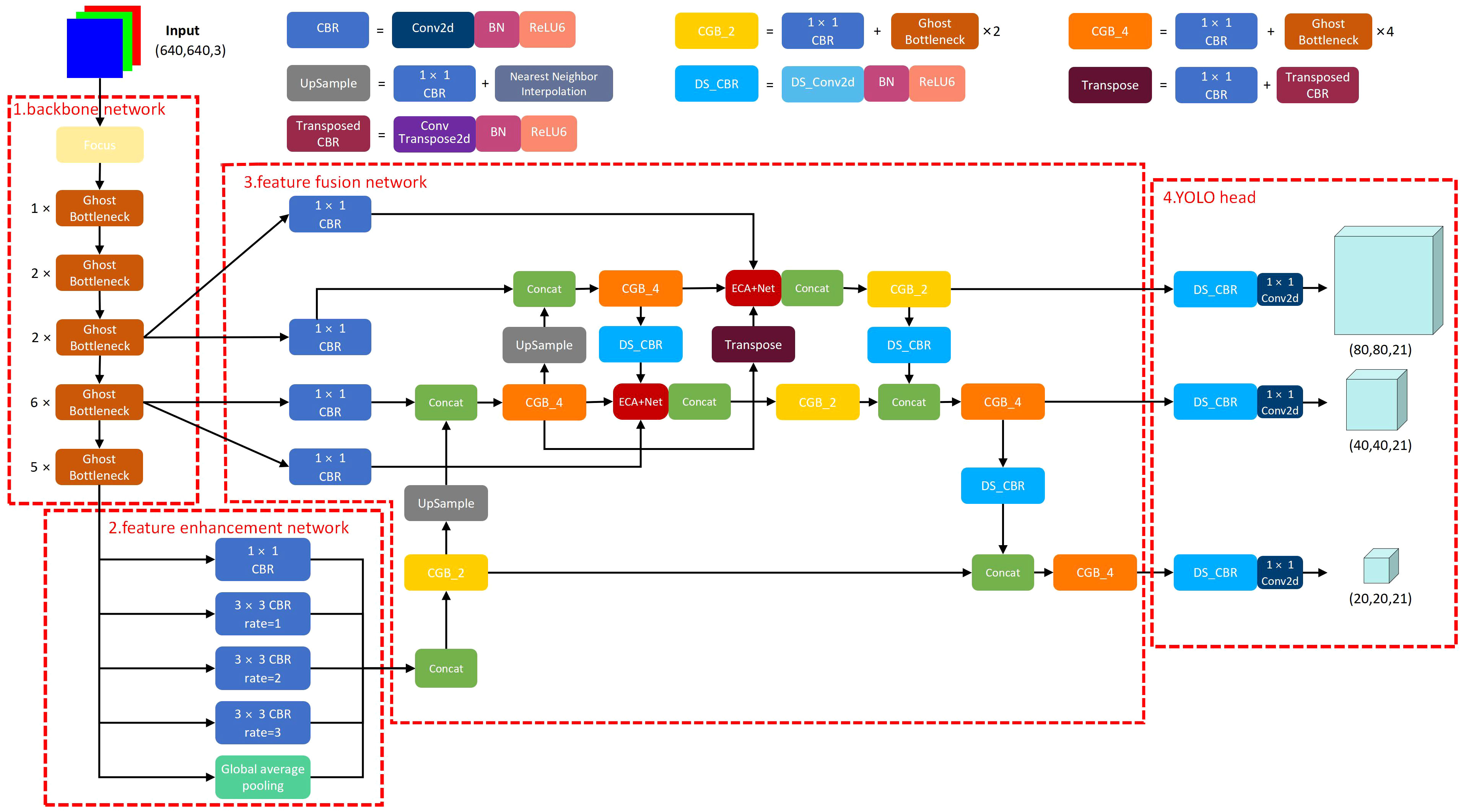
Figure 1 Structure of the GED-YOLO model.
2.2 ECA+GhostNet
The regular convolutions produce many similar feature maps during feature extraction, which are usually considered as redundant information. This redundant information increases the model’s parameters and reduces the model’s efficiency. GhostNet greatly alleviates the feature redundancy issue by using Ghost modules instead of regular convolutions. The process for the Ghost module can be divided into three parts: (1) Use a 1 × 1 convolution for feature integration to build the necessary concentration feature layer; (2) use multiple depth-wise convolutions to generate more Ghost feature layers; and (3) concatenate the feature layers created in the first two stages and output the concatenated result. The structure of the Ghost module is shown in Figure 2A.
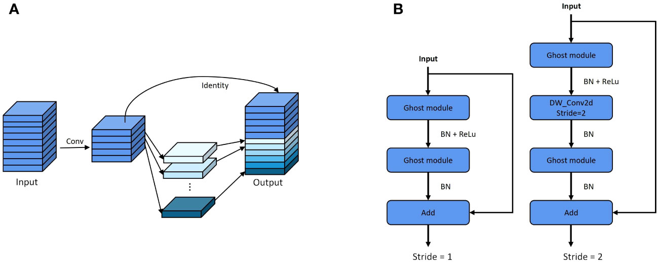
Figure 2 (A) Structure of the Ghost module. (B) Structure of the Ghost bottleneck.
The Ghost bottleneck is the basic component of GhostNet and can be used as a reusable feature extraction module. Similar to the basic residual block in ResNet (He et al., 2016), the Ghost bottleneck also has the residual module, as shown in Figure 2B. The first Ghost module is used as an extension layer to increase the number of network channels and obtain more feature information. The second Ghost module is the concatenate layer, which reduces channel numbers and contacts with the shortcut’s feature layer. The Ghost bottlenecks with different strides are constructed by using depth-wise convolutions to change the size of the feature layer. And the GhostNet is stacked by multiple Ghost bottlenecks with different strides.
In GhostNet, there are several attention networks to help the network perform feature extraction, but the original attention network has many parameters and is inefficient. This paper introduces the Efficient Channel Attention network (ECA-Net) (Wang et al., 2020), which is lighter and more efficient than the original Squeeze-and-Excitation network (SENet) (Hu et al., 2018). The ECA-Net uses 1D convolutions to learn channel feature information. Moreover, ECA-Net uses each channel and its K nearest neighbor channels to obtain local cross-channel interaction information. Using this attention network can improve network efficiency and accelerate network operations. The adaptive-size convolution kernel K is calculated as follows.
In this formula, C represents the total number of input channels, |x|odd represents the nearest odd number to x, γ is set to 2, and b is set to 1. Then, the obtained feature layer is activated through the sigmoid function and multiplied by the original feature layers, as shown in Figure 3A. The sigmoid activation function is formulated as follows.
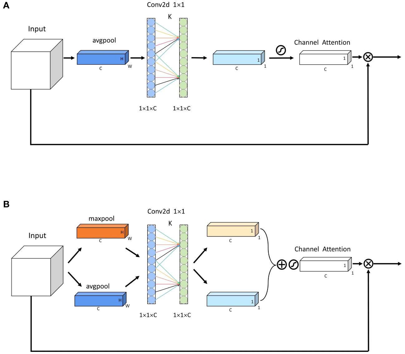
Figure 3 (A) Structure of the ECA-Net. (B) Structure of the ECA+Net.
ECA-Net is both lightweight and efficient; however, the network still misses some eddy information when extracting the channel feature information. Accordingly, a new attention network, ECA+Net, is proposed, which can obtain more comprehensive channel feature information than the original network. ECA+Net processes the input feature layers with average pooling and maximum pooling, learns channel feature information separately by 1D convolutions, sums the learning results, and activates the feature layers through the sigmoid function, as shown in Figure 3B. And the structure of ECA+GhostNet is shown in Table 1.
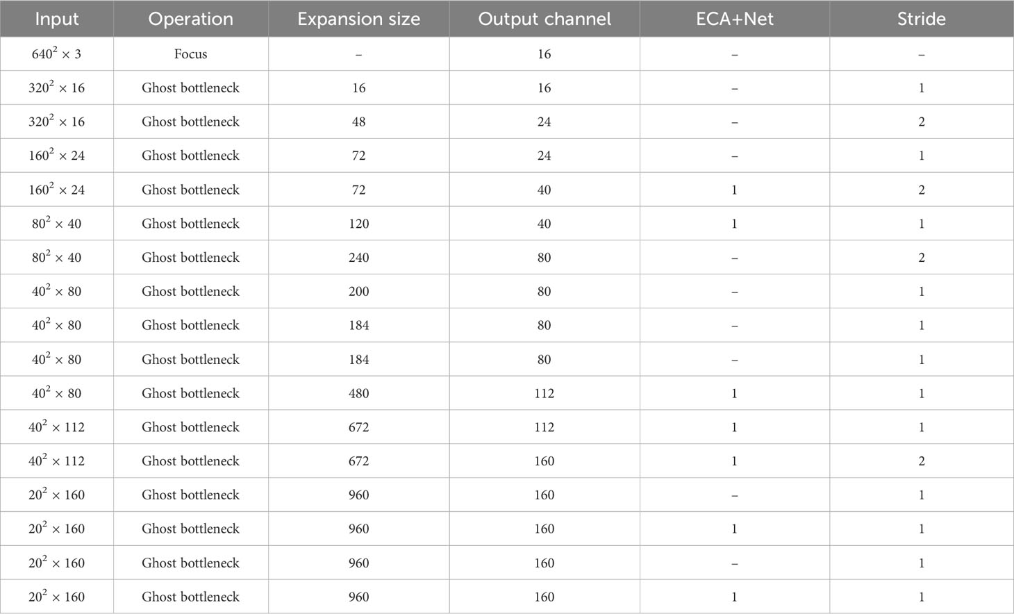
Table 1 Structure of the ECA+GhostNet.
2.3 ASPP
With the development of new object detection methods, the backbone network has become increasingly deeper. However, the increase in the network depth increases the network’s receptive field, which may lead to a loss of feature information for small-scale eddies. This paper uses the dilated convolution (Chen et al., 2018) with small dilation rates to enhance the small-scale eddy features. This convolution method can obtain more ocean eddy feature information by expanding the interval between the convolution kernels. According to the ocean eddy size, convolutions with dilation rates of 1, 2, and 3 are selected to construct the small-target ASPP network.
The ASPP network consists of five modules: a convolution block, three dilated convolution blocks, and a global average pooling block. Among them, the convolution block and dilated convolution blocks are constructed with the convolution + batch normalization + ReLU6 activation function (CBR) modules. The convolution kernel size of the convolution block is 1 × 1, and the convolution kernel size of the dilated convolution blocks is 3 × 3. Moreover, to prevent the loss of ocean eddy feature information caused by large-span convolutions, this ASPP network removes the convolution module and directly outputs the 5 channels’ feature layers. This operation simplifies the network operation process and reduces the loss of eddy feature information.
2.4 GED-PANet
To address the insufficient eddy feature extraction performance of existing lightweight backbone networks, a new feature fusion network, GED-PANet, is proposed based on the PANet. This network integrates the eddy features by repeatedly extracting and concatenating the feature layers that are output by the backbone network and the feature enhancement network. The structure of GED-PANet is shown in Figure 4.
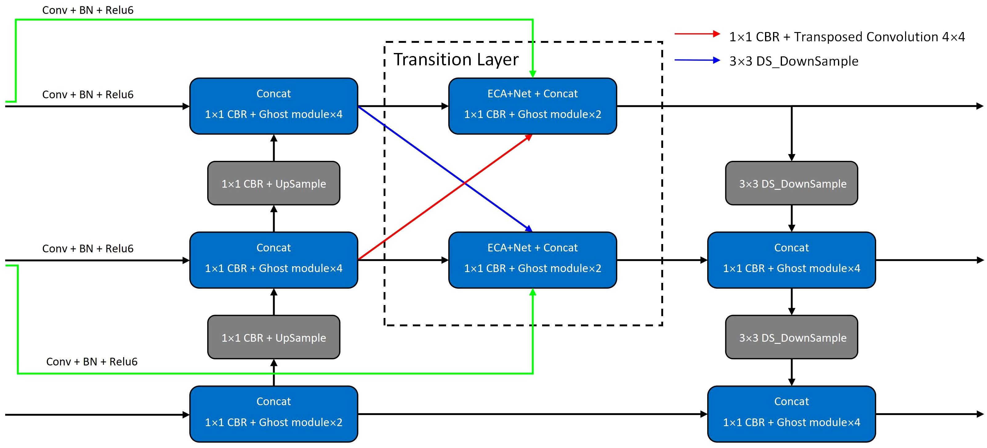
Figure 4 Structure of the GED-PANet.
In the bidirectional feature pyramid network (BiFPN) (Tan et al., 2020), skip connections between different feature layers are used to improve the feature fusion results. Therefore, in the GED-PANet, we also use skip connections to improve small-scale and medium-scale eddy feature layers, as shown by the green lines in Figure 4. To enhance the feature correlation between ocean eddies in different layers, the network uses transposed convolutions and depthwise separable convolutions for cross-layer feature fusion, as shown by the blue and red lines in Figure 4. Using these cross-layer sampling methods leads to more diverse eddy features, thus improving the network performance. And due to the effect of checkerboard artifacts (Odena et al., 2016), the transposed convolution with a kernel size of 4 × 4 and a step size of 2 is selected.
The problem of feature fusion clutter is alleviated by adding a transition layer, as shown by the dotted line region in Figure 4. This transition layer consists of ECA+Nets, convolution modules, and Ghost modules. When the network integrates eddy features, the attention networks produce weights that can be used to determine the features’ contributions. Then, the network accurately integrates the eddy features according to the weighted contributions.
Additionally, to reduce the number of network parameters, GED-PANet uses Ghost modules and depthwise separable convolutions instead of regular convolutions. The 3 (or 5) convolution blocks are changed into one 1×1 convolution block with 2 (or 4) Ghost modules. The 1×1 convolution block is used to adjust the number of channels, and the Ghost modules are used for feature fusion and feature extraction.
2.5 Loss function
The loss function of GED-YOLO consists of Classes loss, Confidence loss, and Location loss. Among them, Classes loss and Confidence loss use the BCELoss. Classes loss is used to calculate the classification loss for samples, while Confidence loss is used to measure the objectness score and the background score. And Location loss uses the CIoU function to calculate the difference between the predicted box and the ground truth box. The loss function for GED-YOLO is as follows, in the formula, Lcls is the Classes loss, Lconf is the Confidence loss, Llocc is the Location loss, and λ is the weighting factor.
The BCELoss function is a classical classification loss function that can effectively classify data samples, and is calculated as follows. p is the prediction result of GED-YOLO, and y is the ground truth.
The CIOU, as an excellent regression loss function, takes the distance between the target and the anchor, the overlap rate, the scale, and the penalty term as the discriminating standards, which makes the target box regression more stable, and does not have the problems such as dispersion during the training process like the IoU and the GIoU. The calculation formulas are as follows.
In the above formulas, IoU is the ratio of the intersection over the union between the predicted box and the ground truth box, which can be used to judge the quality of the prediction results. b and bgt represent the center points of the prediction box and the ground truth box, respectively, ρ2 is the Euclidean distance between the two center points, and c is the diagonal distance of the smallest enclosed area that contains both the prediction box and the ground truth box. And αv is the predicted box aspect ratio fitting the aspect ratio of the ground truth box. Among them, α is a balancing parameter and v is a parameter used to measure the consistency of the aspect ratio.
3 Experimental preparation
3.1 Dataset
The data used in this paper is Level 4 SLA data published by the Copernicus Marine Environment Monitoring Service (CMEMS) (https://marine.copernicus.eu/), which is a global product from multiple satellite altimeter data fusion. The spatial resolution of the data is 0.25°, the temporal resolution is one day, and the data format is NetCDF.
The sea area of 10°N–30°N, 120°E–150°E, which is in the northwest Pacific Ocean, was selected as the dataset area, as shown in Figure 5. And the SLA data from 2017–2020 were selected as the experimental data. This data contains SLA information for different years, seasons, and months. It can well reflect the shape characteristics of ocean eddies and has good time coherence and data complexity. We also plotted the contours of the data to highlight the eddy shape features. Then, we manually labeled the dataset using labelImg software, labeling cyclonic eddies as CE and anticyclonic eddies as AE. LabelImg is a common image annotation tool for object detection, which is written in Python and uses Qt as the graphical interface. The software can store labeled eddies as XML files to support subsequent model training. In addition, to ensure the accuracy of the ocean eddy annotations, we asked experts to review and validate the manual annotations. As for the labeling criterion of the eddies in the dataset, the experts made a comprehensive decision by combining the flow velocity data of the labeled area with the eddy detected by the PET method. Then, the eddies that were wrongly labeled by the human eye were manually eliminated to ensure the accuracy of the eddy dataset.
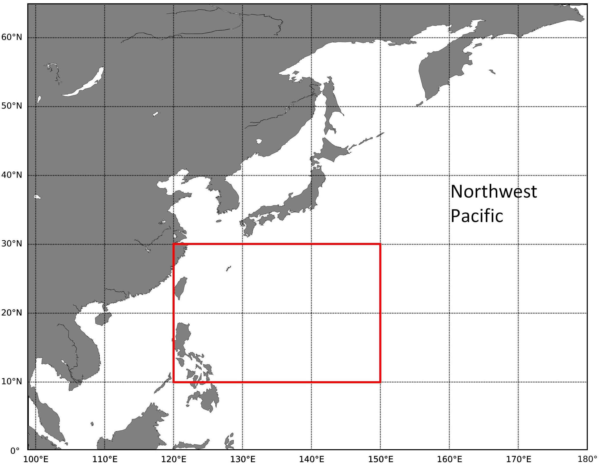
Figure 5 The dataset area (10°N–30°N, 120°E–150°E).
After the experts’ validation, we divided the dataset into the training part, validation part, and testing part. Training part: data used for model training. Validation part: data used for model hyper-parameter tuning. Testing part: data used for model generalizability judgment. The ratio of the training part to the validation part was 9:1, and the ratio of the training samples (training and validation parts) to the testing part was also 9:1. Finally, 1182 training images, 132 validation images, and 147 testing images were obtained.
3.2 Evaluation indices
This paper used Precision, Recall, F1 score, Average Precision (AP), and mean Average Precision (mAP) as the evaluation indices. The Precision is the proportion of correct model-identified samples among all model-identified samples. The Recall is the proportion of correct model-identified samples among all correct samples. The F1 score is the harmonic average of precision and recall. The AP refers to the area under the precision-recall (P-R) curve, which can be used to evaluate the robustness and generalizability of the training results. The mAP is the average of the APs for each class. The calculation formulas for the evaluation indices are as follows.
In these formulas, TP is the number of correct samples identified as correct, FP is the number of incorrect samples identified as correct, FN is the number of correct samples identified as incorrect, P is the precision, R is the recall, and N is the number of sample classes. In addition, we calculate the GFLOPS values for each model. GFLOPS means Giga Floating-point Operations Per Second, which can be used to measure the model’s computational complexity.
3.3 Experimental device and software
The experimental algorithms in this paper were built using Python 3.7 and Pytorch 1.7.1 framework. The program used the Anaconda3 virtual environment and the CUDA version was 11.0. As for the software packages, we used Scipy version 1.2.1, Numpy version 1.17.0, and Matplotlib version 3.1.2. For hardware, the CPU of the experimental computer is AMD Ryzen 7 5800X8-Core processor, the memory of the experimental computer is 32 GB, and the graphics card is NVIDIA GeForce RTX 3080 12G.
4 Experiments and analysis
4.1 Ablation experiments and analysis
To evaluate the impact of each improvement on the proposed model, we conducted step-by-step ablation experiments based on the original GhostNet-YOLO model (Chen et al., 2022). Due to the small size of the eddies relative to the dataset images, this experiment belongs to small and medium target detection. To better extract the image features of the eddies, the large patch size of 640 × 640 was chosen in this experiment. During model training, if the batch size is too small, it will cause the flat minimizers, which in turn will lead to the loss function oscillating without converging the ladder, and if the batch size is too large, it will cause the sharp minimizers, which in turn will lead to the poor model generalization ability (Keskar et al., 2016). GPUs can perform better with batch sizes that are powers of 2. Considering the size of the dataset and the computer hardware, the batch size was set to 16. In this experiment, the initial learning rate was set to 0.01, the optimizer was the Adam optimizer, and the momentum parameter was 0.9. During the training process, we set the weights to be saved every 5 epochs of training, used the Mosaic data enhancement method, used the Cosine Annealing Learning Rate, used single-GPU training mode, did not parallelize the computation, and set the total epoch to 50. Finally, the training took 3 hours and 16 minutes. The loss change image of the training process is shown in the Supplementary Material.
Table 2 shows the changes in mAP for the ablation experiments, and it can be seen that the use of ECA+GhostNet increased the mAP by 0.7%. The small-target ASPP network enhanced the model’s ability to extract ocean eddy features, and the addition of this network increased the mAP by 0.26%. Using the GED-PANet significantly improved the eddy detection performance, increasing the mAP by 1.52%. Overall, compared to the mAP of the original model, the mAP of GED-YOLO increased by 2.48%.
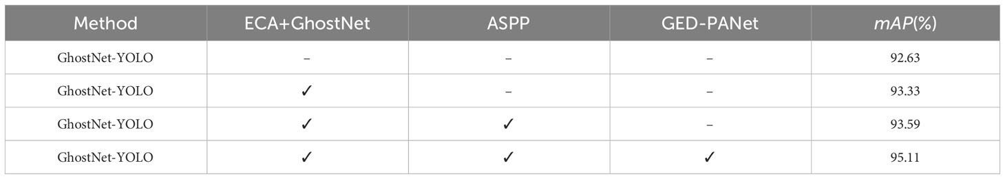
Table 2 Results of the ablation experiments.
4.2 Comparison experiments and analysis
To evaluate the eddy detection performance of GED-YOLO, we compared our model to other models. Due to the large differences in the detection principles of different structure models, some limitations are imposed on the models’ quantitative analysis. For example, the two-stage object detection model generates 9 priority bounding boxes during the prediction process, while the one-stage model only generates 3 priority bounding boxes, which creates some limitations in analyzing the same modules in different models. Therefore, in this experiment, we used the YOLO framework’s model as the baseline model and selected a lot of YOLO models for experiments. The results of the comparison experiments are shown in Table 3.
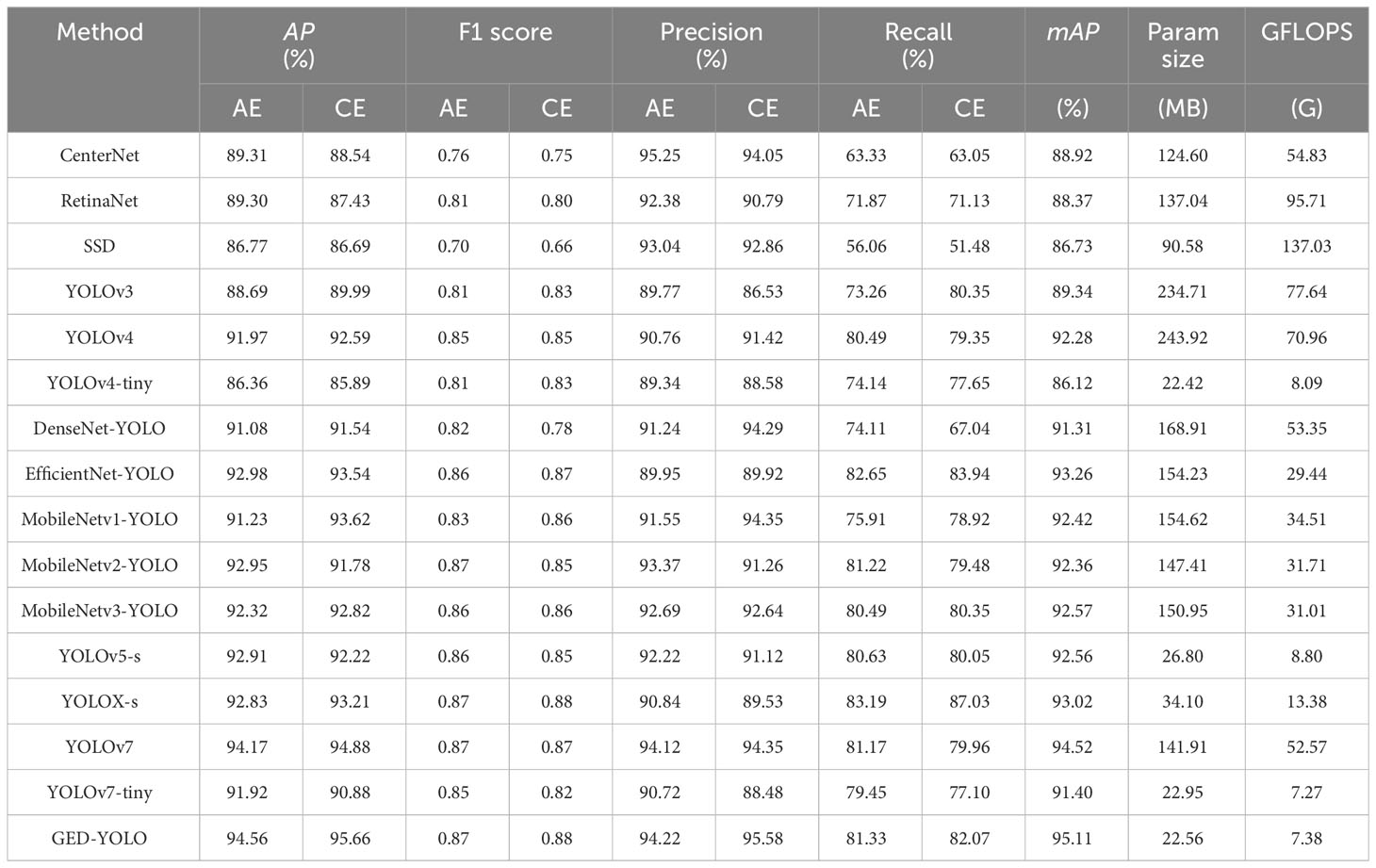
Table 3 Results of the comparison experiments.
First, GED-YOLO had the highest AP values of 94.56% and 95.66% among all models. Compared to YOLOv7 (Wang et al., 2022a), the AP value of GED-YOLO was 0.39% higher for anticyclonic eddies and 0.78% higher for cyclonic eddies. Second, GED-YOLO and YOLOX (Ge et al., 2021) had the highest F1 scores among all models. Both had F1 scores of 0.87 for anticyclonic eddies and 0.88 for cyclonic eddies. CenterNet (Duan et al., 2019) had the highest precision of 95.25% for anticyclonic eddies, and GED-YOLO had the highest precision of 95.58% for cyclonic eddies. And the average value of GED-YOLO’s precision is 0.25% higher than CenterNet’s. YOLOX had the highest recall scores of 83.19% and 87.03%. However, the difference in the recall between anticyclonic eddies and cyclonic eddies was 3.84%, which might lead to an imbalance in the detection of different classes of eddies. Furthermore, GED-YOLO had the highest mAP among the comparison models, with an mAP of 95.11%. The model parameter size of GED-YOLO was 22.56 MB, which was significantly lighter than traditional models. Although the parameter size of GED-YOLO was 0.14 MB larger than that of YOLOv4-tiny, its detection performance was significantly better. The GFLOPS values of GED-YOLO, YOLOv7-tiny, YOLOv5-s, and YOLOv4-tiny were significantly lower than those of the traditional large-scale models. This indicated that these lightweight models had low computational complexity. And among these lightweight models, GED-YOLO had a higher mAP value. In addition, the result of the graphical visualization of the different models’ complexity and mAP is presented in the Supplementary Material.
Figure 6 shows the eddy detection results on January 1, 2017, for different models. In the figure, the red boxes represent anticyclonic eddies and the blue boxes represent cyclonic eddies. It can be seen that the eddies detected by GED-YOLO, YOLOX-S, and YOLOv7 were in high consistency with the eddies in the ground truth.
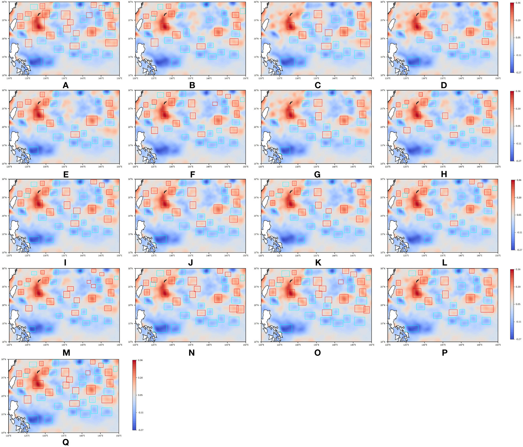
Figure 6 The detection visualization results of comparison experiments on January 1, 2017. (A) Ground truth. (B) CenterNet. (C) RetinaNet. (D) SSD. (E) YOLOv3. (F) YOLOv4. (G) YOLOv4-tiny. (H) DenseNet-YOLO. (I) EfficientNet-YOLO. (J) MobileNetv1-YOLO. (K) MobileNetv2-YOLO. (L) MobileNetv3-YOLO. (M) YOLOv5-s. (N) YOLOX-s. (O) YOLOv7. (P) YOLOv7-tiny. (Q) GED-YOLO.
Overall, the eddy detection performance of GED-YOLO was better than the other structural models, including CenterNet, SSD (Liu et al., 2016), and RetinaNet (Lin et al., 2017). GED-YOLO also had better training results than the other YOLO series models, such as YOLOv3 (Redmon and Farhadi, 2018), YOLOv4 (Bochkovskiy et al., 2020), and YOLOv5-s. Moreover, GED-YOLO extracted eddy features better than DenseNet (Huang et al., 2017), EfficientNet (Tan and Le, 2019), and MobileNet series (Howard et al., 2017; Sandler et al., 2018; Howard et al., 2019) models. And compared with other lightweight models, such as YOLOv4-tiny and YOLOv7-tiny, GED-YOLO did show better eddy detection performance.
4.3 Generalization experiments and analysis
For a more comprehensive analysis of GED-YOLO’s eddy detection performance, we carried out generalization experiments. We calculated and plotted the graphical visualization of GED-YOLO eddy detection performance, as shown in Figure 7.
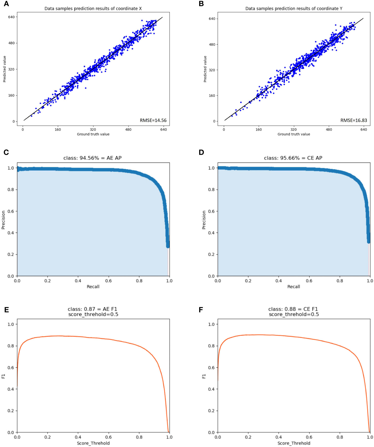
Figure 7 The Graphical visualization of GED-YOLO detection performance. (A) Predicted results for the eddies center points coordinate X. (B) Predicted results for the eddies center points coordinate Y. (C) Results of AP graphical visualization of anticyclonic eddies. (D) Results of AP graphical visualization of cyclonic eddies. (E) Results of F1 graphical visualization of anticyclonic eddies. (F) Results of F1 graphical visualization of cyclonic eddies.
We geometrically computed the GED-YOLO predictions in the testing part to obtain the coordinates (X, Y) of the eddy centers. After that, the predicted X-values and Y-values were compared with the center points calculated by Ground truth, and the A and B graphs were obtained. It can be seen in Figure 7A that there were significantly fewer points in the range of X-values from 0 to 160 than in the other ranges. This was because the dataset had land in that range. And in Figure 7B, the points in the range of 0 to 320 were less than those in the range of 320 to 640. This was because the range of 0 to 320 was located in the sea area of 10°N to 20°N, and the number of eddies near the equator was less than that in the higher latitudes.
As can be seen from C and D in Figure 7, GED-YOLO performed well in precision and recall and had a good balance in eddy detection. E and F in Figure 7 are the F1 Score and score threshold curves. These two curves showed that GED-YOLO was stable in the eddy detection. Therefore, GED-YOLO showed good performance in eddy detection and index parameters evaluation.
4.4 Uncertainty experiments and analysis
Currently, deep learning models have been fully applied in various fields, but the models still have some uncertainty in the process of prediction (Gawlikowski et al. 2023). Therefore, to sufficiently test the robustness and generalizability of the model, we carried out model uncertainty experiments on the GED-YOLO.
Firstly, we carried out the uncertainty experiment of the experimental data. We first added noise to the images of 2017 and 2019 in the dataset and mixed them with the original 2018 and 2020 images to produce a dataset with 50% noise content. And we added noise to the images of 2018 and 2020 to make a dataset with 100% noise content. Then, we obtained three datasets with 0%, 50%, and 100% noise content and retrained these datasets separately using GED-YOLO. The mAP values of GED-YOLO on 0%, 50%, and 100% were 95.11%, 95.14%, and 95.04%, respectively. The detection results for each dataset are shown in Figure 8. It can be seen that the detection performance of GED-YOLO on the same dataset for original and noisy images was stable, and the eddy detection results were highly consistent. As shown in Figures 8A and D, the GED-YOLO trained on the dataset with 0% noise content had the same eddy detection results on both images. However, there was still uncertainty in GED-YOLO for training on different datasets. As can be seen from A, B, and C in Figure 8, there were still small differences in eddy detection by GED-YOLO for the different datasets. And it can be found from the figure that there were subtle differences in the prediction of the eddy size by the GED-YOLO model. To better balance the uncertainty, we calculated the average value and sample standard deviation of the mAP for different datasets. Ultimately, the mAP of the data uncertainty experiment was 95.10%, and the sample standard deviation of the mAPs was 0.0513.
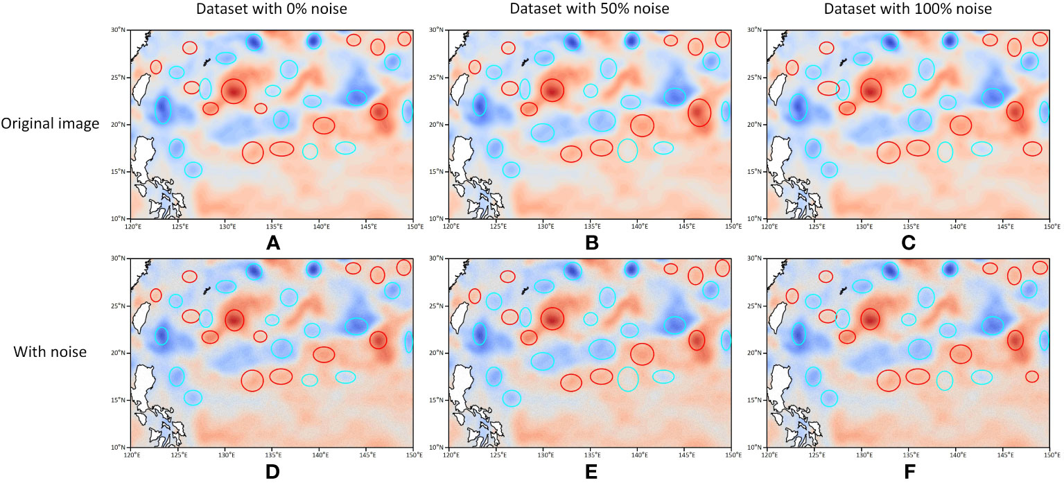
Figure 8 Detection results of data uncertainty experiments. (A) Results of detecting the original image with 0% noise dataset. (B) Results of detecting the original image with 50% noise dataset. (C) Results of detecting the original image with 100% noise dataset. (D) Results of detecting the noisy image with 0% noise dataset. (E) Results of detecting the noisy image with 50% noise dataset. (F) Results of detecting the noisy image with 100% noise dataset.
Secondly, we carried out the model uncertainty experiment for GED-YOLO. We perturbed the model weights by loading the pre-trained weights. Before the experiment, we trained the VOC 2012 dataset and our dataset to produce the pre-trained weights. Different from the direct training model, loading the pre-trained weights can make the original model weights perturbed and make the model weights more orderly in training. We conducted uncertainty experiments using the model without loaded pre-trained weights, the model loaded with VOC 2012 pre-trained weights, and the model loaded with our dataset’s pre-trained weights. And we observed the model uncertainty by comparing the training results with different weights. It can be seen in Table 4 that the pre-trained weights of the VOC 2012 dataset and our dataset slightly improved the training results. And the mAP of the freeze training model is smaller than that of the unfreeze training model. This was because the weight of the backbone network didn’t change during the freezing training, resulting in a slower increase in the mAP. The average mAP of the freeze training result was 94.87%, and the sample standard deviation was 0.0346. The average mAP of the unfreeze training result was 95.13%, and the sample standard deviation was 0.0208.
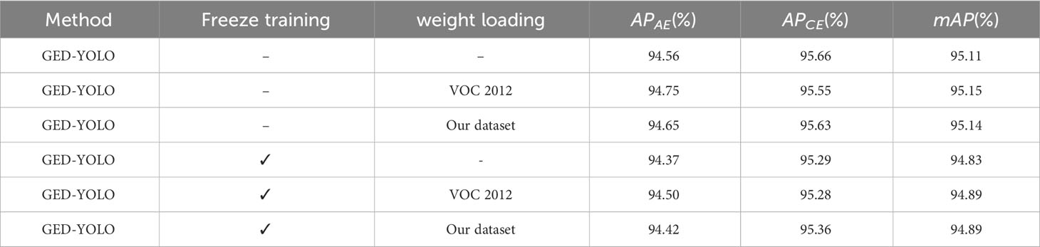
Table 4 Experimental results of the model uncertainty.
We also conducted the distributional uncertainty experiment. In this experiment, we divided the training samples and the testing part according to the ratios of 9:1, 8:2, and 7:3. To make the data of training samples and testing part interchangeable, we redivided the dataset. Specifically, we redistributed data from the training samples to the testing part and retrained the model. We analyzed the uncertainty by training on datasets of different scales and divisions. As can be seen in Table 5, the training results with a ratio of 9:1 were better than those with a ratio of 8:2, while the training results with a ratio of 8:2 were better than those with a ratio of 7:3. In addition, we found that redividing the dataset caused uncertainty in GED-YOLO. So we calculated mAP average values and sample standard deviations as experimental results for datasets with ratios of 9:1, 8:2, and 7:3. The mAPs of the distributional uncertainty experiments were 95.10%, 94.24%, and 93.56%, and the sample standard deviations were 0.0208, 0.0351, and 0.0404, respectively.
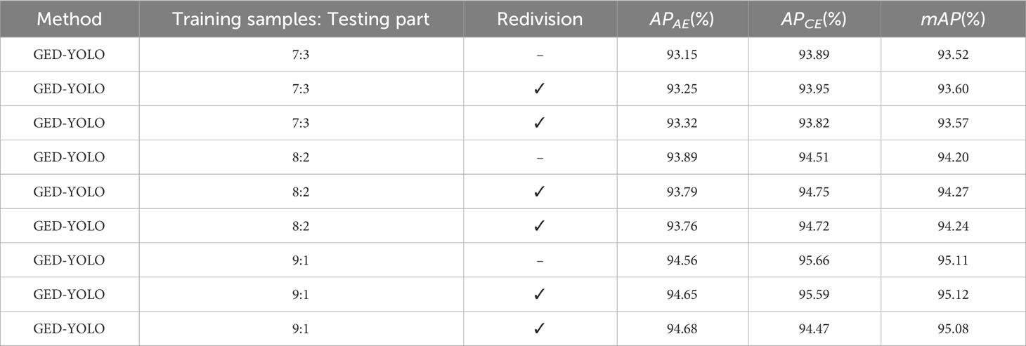
Table 5 Experimental results of the distributional uncertainty.
4.5 Detection experiments and analysis
In this paper, we also conducted detection experiments to test the usefulness of GED-YOLO. We selected four different deep learning models, CenterNet, YOLOv4, YOLOX-s, and GED-YOLO, for detection experiments. And the data for the area of 10°N–30°N, 120°E–150°E in 2021 were selected as experimental data. We used data that were not in the dataset for these experiments to better test the usefulness of the models. The detection results for different periods are shown in Figure 9. The results show that GED-YOLO and YOLOX-s detected more ocean eddies than YOLOv4 and CenterNet, and the detection confidences of GED-YOLO and YOLOv4 were higher than those of YOLOX-s and CenterNet.
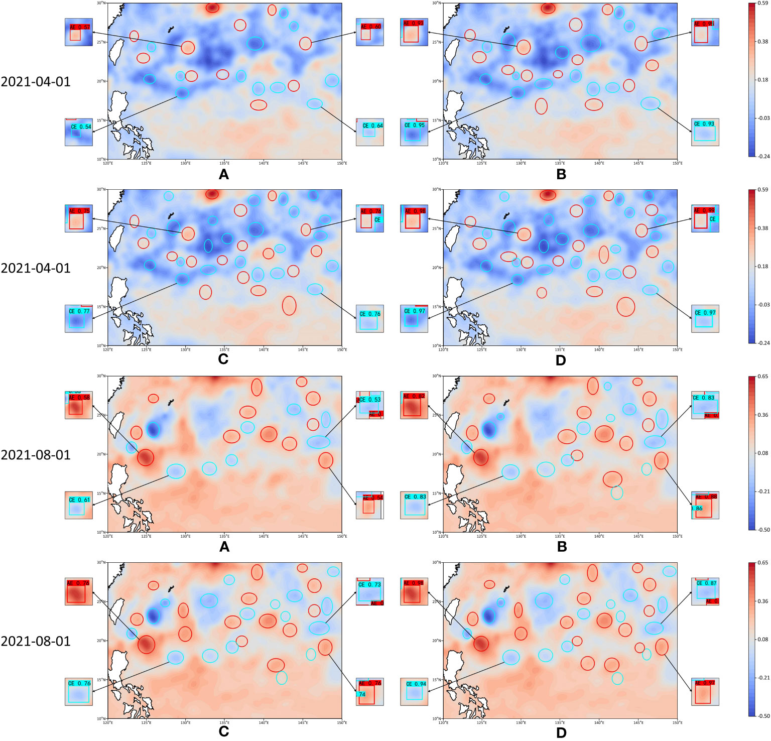
Figure 9 The detection results of four models. (A) CenterNet. (B) YOLOv4. (C) YOLOX-s. (D) GED-YOLO.
Figure 10 presents the eddy statistics detected by the four methods based on 2021 data. YOLOX-s and GED-YOLO detected more ocean eddies than YOLOv4 and CenterNet. However, compared with the results of the other three models, the detection results of YOLOX-s showed large anomalous fluctuations from July to November. Furthermore, the proportion of different classes of eddies detected by YOLOX-s differed by approximately 2.4% from the results of the other models, as shown in Table 6. The main reason for this anomaly was the large divergence in the recall of YOLOX-s for different classes of eddies. In contrast, the eddy detection results of the other three models were more stable. In general, GED-YOLO had good detection performance, suggesting that GED-YOLO could be used as a reliable deep learning ocean eddy detection model.
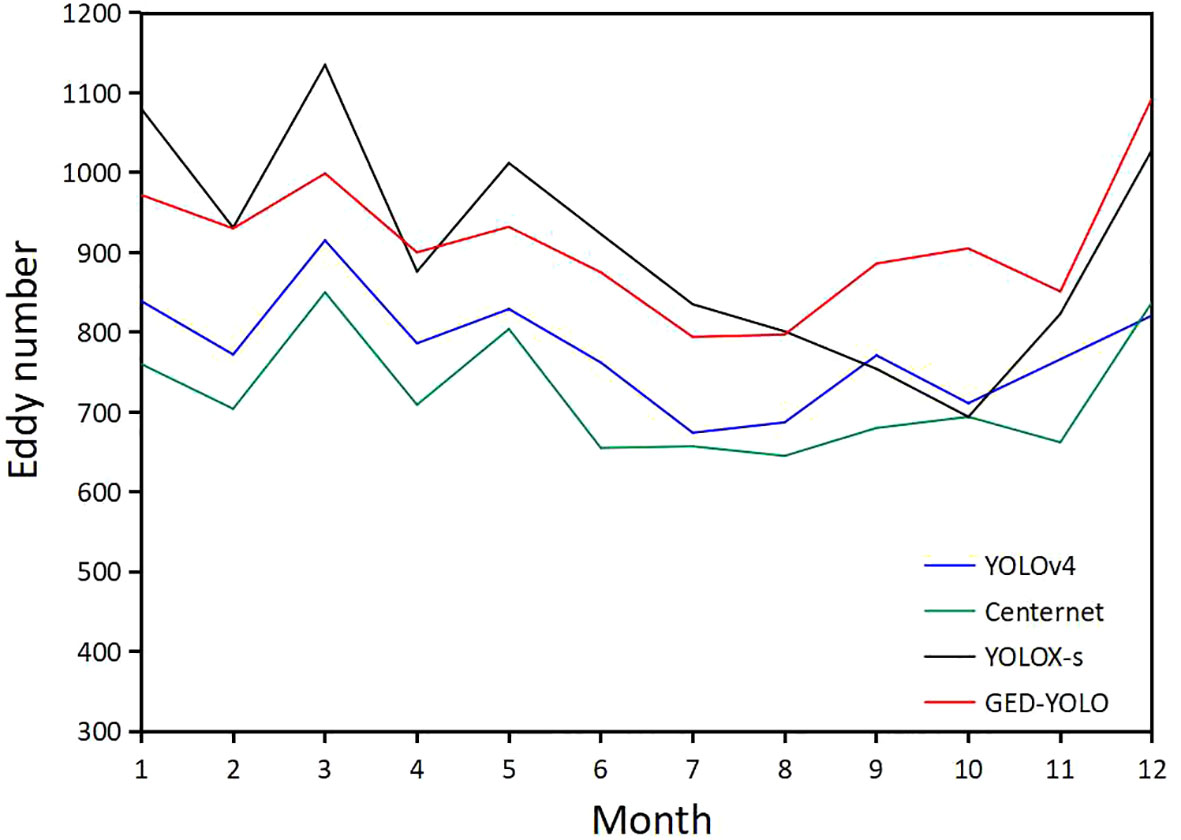
Figure 10 Statistical chart of eddy detection results in 2021.
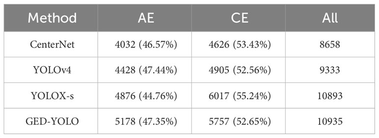
Table 6 Statistical table of the total number of detected eddies in 2021.
4.6 Test experiments and analysis
4.6.1 Regional test experiments
To test the accuracy of GED-YOLO in detecting eddies, this study compared the detection results of GED-YOLO with those of the physical-based method. The criterion for GED-YOLO to detect ocean eddies is the geometric features of the closed contours of the SLA data, which belongs to the category of Eulerian eddy detection. Therefore, for a better quantitative comparison, we chose the PET method, which detects ocean eddies also by the sea surface closed profiles, for experiments. In addition, to evaluate the experiment results, we manually examined the different detected eddies by the geostrophic flow.
The detection results for the Indian Ocean area (30°S–45°S, 100°E–120°E) on December 1, 2021, are shown in Figure 11. In this figure, the black dotted line areas are the areas detected by GED-YOLO but not by the PET, the black solid line areas are the areas detected incorrectly by GED-YOLO, the green dotted line areas are the areas detected by the PET but not by GED-YOLO, and the green solid line areas are the areas detected incorrectly by the PET.
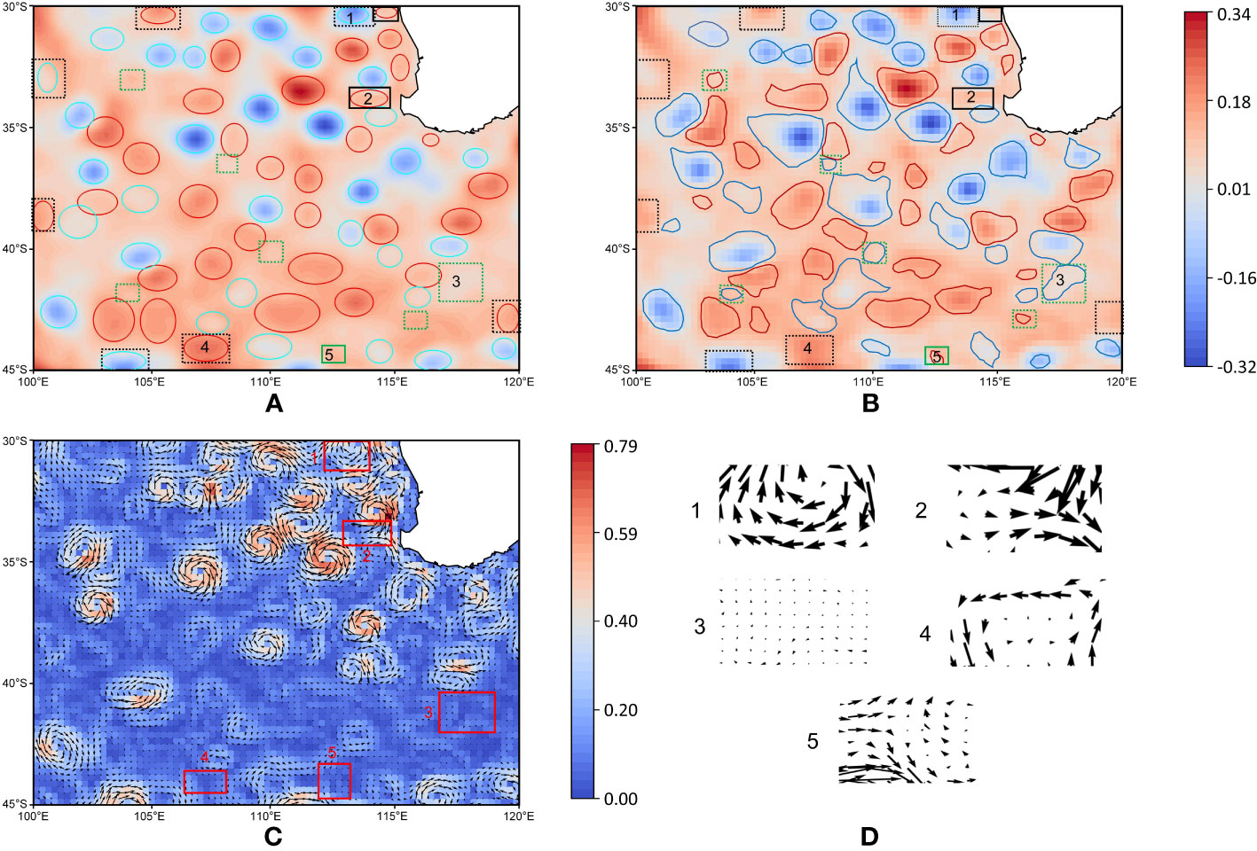
Figure 11 Test results in the Indian Ocean area. (A) GED-YOLO. (B) PET. (C) Geostrophic flow. (D) Regional geostrophic flow.
The figure shows that the boundary detection performance of GED-YOLO was better than that of PET, as shown in regions 1 and 4 in Figure 11. However, due to insufficient contour drawings, GED-YOLO had poor detection performance for small-amplitude eddies. As shown in region 3 in Figure 11, the image failed to draw a closed contour feature for the eddy in this area, resulting in the loss of eddy detection. In addition, GED-YOLO had eddy detection errors in areas near the mainland. The errors in the regions were caused by the impact of the coastline and seafloor topography, causing sea surface anomalies and creating pseudo-eddies, which eventually led to eddy detection errors. As shown in region 2 in Figure 11, the complex coastline led to the formation of strong opposite currents that produced sea surface anomalies similar to eddies, resulting in eddy detection errors. In the open ocean, GED-YOLO could remove the pseudo-eddies, as shown in region 5 in Figure 11. In terms of the eddy detection speed, PET needed 2–3 seconds to detect ocean eddies for one day, while GED-YOLO only needed 0.14 seconds. We also counted the detection results of these two methods for December 2021 and calculated the correlation coefficient. The correlation coefficient is calculated as follows.
The statistical results are shown in Figure 12. The number of ocean eddies detected by the two methods was highly consistent. And the correlation coefficient between GED-YOLO and PET was 0.93, which means that the two methods had a strong correlation.
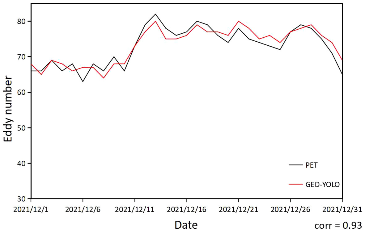
Figure 12 Statistical chart of test results in the Indian Ocean area.
For the Atlantic Ocean area (30°N–50°N, 10°W–40°W) and the Pacific Ocean area (20°N–40°N, 120°W–150°W), GED-YOLO also showed good ocean eddy detection performance, and results of the test on December 1, 2021, are shown in Figure 13. As in the Indian Ocean test experiment, in Figure 13, the solid line areas indicate the areas that were incorrectly detected by the two methods, and the dotted line areas indicate the areas in which one method detected more eddies than the other method. In the open ocean, the detection performance of these two methods was similar, and in the boundary areas, GED-YOLO had a better detection performance than PET. The detection speed of GED-YOLO was 0.14 seconds for one day of data, which was much faster than the 2–3 seconds needed by PET for the same amount of data. However, the ability of GED-YOLO to detect small-amplitude eddies was still poor due to insufficient contour drawing.
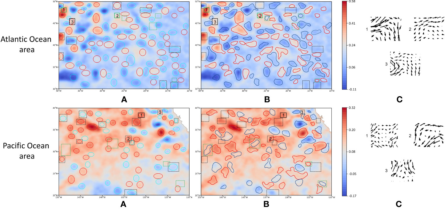
Figure 13 Test results in the Atlantic Ocean area and the Pacific Ocean area. (A) GED-YOLO. (B) PET. (C) Regional geostrophic flow.
In addition, we also carried out experiments for the eddy detection method based on another physical principle. The Lagrangian eddy detection method (Haller and Beron-Vera, 2013) is one of the most trustworthy methods for eddy detection based on the rotating flow field characteristics of eddies. We compared the detection results of the Lagrangian, PET, and GED-YOLO, as shown in Figure 14. It can be seen in the figure that the Lagrangian method detected eddies with smoother boundaries than PET, and the size of the detected eddies is relatively smaller. Although the number of eddies detected by the Lagrangian method was less than that of PET and GED-YOLO, the accuracy of eddy detection was higher. As shown in region 1 of the figure, both PET and GED-YOLO showed errors in eddy detection. This was due to the sea surface anomalies caused by the complex currents in the region, which produced a pseudo-eddy. And this pseudo-eddy behaved the same as normal eddy in the SLA data, which in turn led to the detection error of PET and GED-YOLO. Moreover, the Lagrangian method was more rigorous in confirming the eddy boundary. As shown in region 2 and region 3, the Lagrangian method could detect the eddy boundaries accurately based on the flow velocity data, while the boundaries detected by the PET method were not appropriate enough. And GED-YOLO did not detect eddies in these two regions. In the boundary region, the detection performance of GED-YOLO was better than that of Lagrangian and PET. As shown in region 4 of Figure 14C, GED-YOLO detected the eddy, while the other two methods did not. This was due to eddies in the boundary region, some of their data being outside the experimental area, which made the computation of the physically-based models incomplete, leading to missing detections. GED-YOLO detected ocean eddy based on the eddy feature in the images, so it did not necessarily require complete eddy data. Therefore, in future work, we will fuse SLA data with velocity data to detect ocean eddies more accurately.

Figure 14 The eddy detection results of the Lagrangian method, the PET method, and the GED-YOLO method. (A) Results of the Lagrangian method. (B) Results of the PET method. (C) Results of the GED-YOLO method. (D) Regional geostrophic flow.
4.6.2 Global test experiments
To adequately assess the model’s accuracy and usefulness, we conducted test experiments on a global scale. We divided the global data for January 1, 2022, into 108 regions based on different sea areas, detected the eddies separately, and combined the detection results. The detection results are shown in Figure 15. PET detected 2289 anticyclonic eddies and 2387 cyclonic eddies, while GED-YOLO detected 2371 anticyclonic eddies and 2456 cyclonic eddies. Among them, 1902 anticyclonic eddies and 1956 cyclonic eddies were detected by both methods, demonstrating consistency rates of 81.63% and 80.78%, respectively.
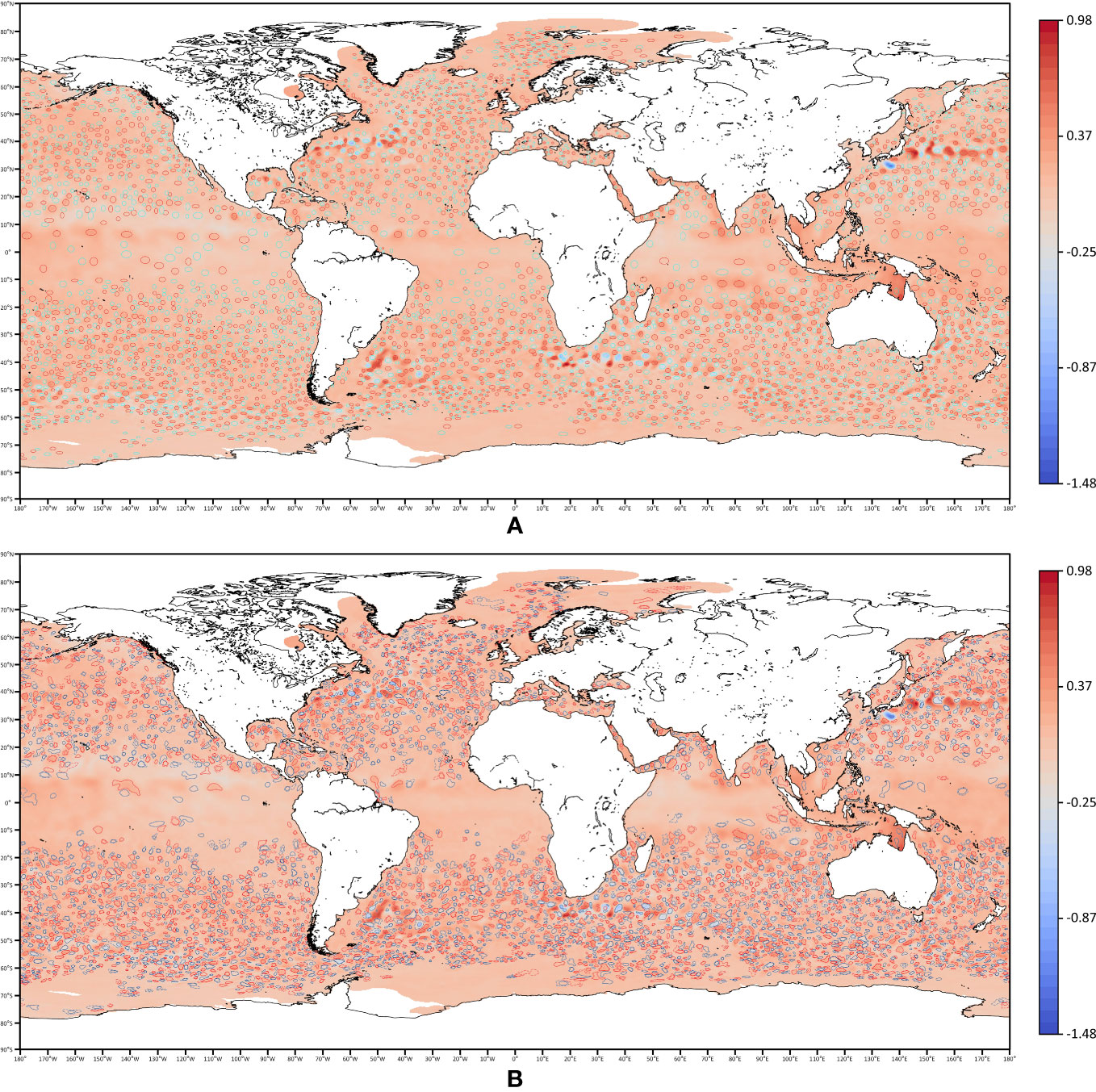
Figure 15 The global ocean eddy detection results. (A) GED-YOLO. (B) PET.
It can be seen in Figure 15 that the eddy detection performance of GED-YOLO was better than that of PET in the area of 10°S–10°N. And GED-YOLO detected the 108 areas in 15 seconds, which was much faster than the PET’s. In addition, PET required complex calculations, such as high-pass filtering and automatic interpolation, to detect ocean eddies. Due to these computational limitations, PET was unstable and often unusable. While GED-YOLO solved this shortcoming well, it could detect ocean eddies quickly and stably.
5 Conclusion
In this study, GED-YOLO, a lightweight and efficient deep learning ocean eddy detection model, was proposed. This model used ECA+GhostNet as the backbone network, a small-target ASPP model as the feature enhancement network, and GED-PANet as the feature fusion network. The SLA data acquired in the region of 10°N–30°N, 120°E–150°E from 2017–2020 were selected as the dataset. The experimental results showed that the mAP of GED-YOLO reached 95.11%, and the model parameter size was 22.56 MB. Compared with other deep learning models, GED-YOLO had better detection performance and lighter model parameter size. And the robustness and the generalizability of the model were also confirmed well by generalization and uncertainty experiments. In test experiments, GED-YOLO showed good eddy detection performance in other areas, including the Indian Ocean area, the Atlantic Ocean area, the Pacific Ocean area, and a global scale. Therefore, GED-YOLO could be applied as a lightweight and reliable deep learning model for ocean eddy detection.
Although GED-YOLO could quickly and stably detect ocean eddies, the model still had shortcomings in small-amplitude eddy detection and eddy boundary determination. Therefore, the development of a more accurate and comprehensive deep learning model for detecting ocean eddies has become the focus of our future research. In future work, we will produce a more detailed eddy dataset to highlight the features of small-amplitude eddies. Then, we will attempt to extract the boundaries of eddies by using instance segmentation models. In addition, we will attempt to fuse multisource and multitype data to detect ocean eddies more accurately.
Data availability statement
The original contributions presented in the study are included in the article/supplementary material. Further inquiries can be directed to the corresponding authors.
Author contributions
HS: Conceptualization, Methodology, Writing – original draft. HL: Conceptualization, Funding acquisition, Methodology, Writing – review & editing. MX: Methodology, Validation, Writing – review & editing. FY: Investigation, Validation, Writing – review & editing. QZ: Data curation, Validation, Writing – review & editing. CL: Validation, Writing – review & editing.
Funding
The author(s) declare financial support was received for the research, authorship, and/or publication of this article. This research is funded by the National Program on Global Change and Air-Sea Interaction (Phase II) – Parameterization assessment for interactions of the ocean dynamic system.
Acknowledgments
The authors would like to thank Copernicus Marine Environment Monitoring Service for the data supplied. The authors would like to thank the editor and reviewers for their comments and suggestions.
Conflict of interest
The authors declare that the research was conducted in the absence of any commercial or financial relationships that could be construed as a potential conflict of interest.
Publisher’s note
All claims expressed in this article are solely those of the authors and do not necessarily represent those of their affiliated organizations, or those of the publisher, the editors and the reviewers. Any product that may be evaluated in this article, or claim that may be made by its manufacturer, is not guaranteed or endorsed by the publisher.
Supplementary material
The Supplementary Material for this article can be found online at: https://www.frontiersin.org/articles/10.3389/fmars.2023.1266452/full#supplementary-material
References
Bai X., Wang C., Li C. (2019). A streampath-based RCNN approach to ocean eddy detection. IEEE Access 7, 106336–106345. doi: 10.1109/ACCESS.2019.2931781
Bochkovskiy A., Wang C.-Y., Liao H.-Y. M. (2020). YOLOv4: Optimal speed and accuracy of object detection. arXiv preprint arXiv doi. doi: 10.48550/arXiv.2004.10934
Cabrera M., Santini M., Lima L., Carvalho J., Rosa E., Rodrigues C., et al. (2022). The southwestern Atlantic Ocean mesoscale eddies: A review of their role in the air-sea interaction processes. J. Mar. Syst. 235, 103785. doi: 10.1016/j.jmarsys.2022.103785
Chaigneau A., Gizolme A., Grados C. (2008). Mesoscale eddies off Peru in altimeter records: Identification algorithms and eddy spatio-temporal patterns. Prog. Oceanogr. 79, 106–119. doi: 10.1016/j.pocean.2008.10.013
Chelton D. B., Schlax M. G., Samelson R. M. (2011). Global observations of nonlinear mesoscale eddies. Prog. Oceanogr. 91, 167–216. doi: 10.1016/j.pocean.2011.01.002
Chelton D. B., Schlax M. G., Samelson R. M., de Szoeke R. A. (2007). Global observations of large oceanic eddies. Geophys. Res. Lett. 34, L15606. doi: 10.1029/2007GL030812
Chen L.-C., Papandreou G., Schroff F., Adam H. (2017). Rethinking atrous convolution for semantic image segmentation. arXiv preprint arXiv. doi: 10.48550/arXiv.1706.05587
Chen L.-C., Papandreou G., Kokkinos I., Murphy K., Yuille A. L. (2018). Deeplab: Semantic image segmentation with deep convolutional nets, atrous convolution, and fully connected CRFs. IEEE Trans. Pattern Anal. Mach. Intell. 40, 834–848. doi: 10.1109/TPAMI.2017.2699184
Chen G., Yang J., Han G. (2021a). Eddy morphology: Egg-like shape, overall spinning, and oceanographic implications. Remote Sens Environ. 257, 112348. doi: 10.1016/j.rse.2021.112348
Chen G., Yang J., Tian F., Chen S., Zhao C., Tang J., et al. (2021b). Remote sensing of oceanic eddies: Progresses and challenges. Natl. Remote Sens. Bull. 25, 302–322. doi: 10.11834/jrs.20210400
Chen W., Zhu G., Mao M., Xi X., Xiong W., Liu L., et al. (2022). “Defect detection method of wind turbine blades based on improved YOLOv4,” in 2022 International Conference on Sensing, Measurement & Data Analytics in the era of Artificial Intelligence (ICSMD) (Harbin, China: IEEE), 1–4. doi: 10.1109/ICSMD57530.2022
Chollet F. (2017). “Xception: Deep learning with depthwise separable convolutions,” in Proceedings of the IEEE Conference on Computer Vision and Pattern Recognition (CVPR) (Hawaii, USA: IEEE), 1251–1258.
D’Alimonte D. (2009). Detection of mesoscale eddy-related structures through iso-SST patterns. IEEE Geosci. Remote Sens. Lett. 6, 189–193. doi: 10.1109/LGRS.2008.2009550
Dong C., Nencioli F., Liu Y., McWilliams J. C. (2011). An automated approach to detect oceanic eddies from satellite remotely sensed sea surface temperature data. IEEE Geosci. Remote Sens. Lett. 8, 1055–1059. doi: 10.1109/LGRS.2011.2155029
Duan K., Bai S., Xie L., Qi H., Huang Q., Tian Q. (2019). “CenterNet: Keypoint triplets for object detection,” in Proceedings of the IEEE/CVF International Conference on Computer Vision (ICCV) (Seoul, Korea: IEEE), 6569–6578.
Dumoulin V., Visin F. (2016). A guide to convolution arithmetic for deep learning. arXiv preprint arXiv. doi: 10.48550/arXiv.1603.07285
Duo Z., Wang W., Wang H. (2019). Oceanic mesoscale eddy detection method based on deep learning. Remote Sens. 11, 1921. doi: 10.3390/rs11161921
Faghmous J. H., Frenger I., Yao Y., Warmka R., Lindell A., Kumar V. (2015). A daily global mesoscale ocean eddy dataset from satellite altimetry. Sci. Data 2, 1–16. doi: 10.1038/sdata.2015.28
Falkowski P. G., Ziemann D., Kolber Z., Bienfang P. K. (1991). Role of eddy pumping in enhancing primary production in the ocean. Nature 352, 55–58. doi: 10.1038/352055a0
Frenger I., Gruber N., Knutti R., Münnich M. (2013). Imprint of Southern Ocean eddies on winds, clouds and rainfall. Nat. Geosci. 6, 608–612. doi: 10.1038/ngeo1863
Gawlikowski J., Tassi C. R. N., Ali M., Lee J., Humt M., Feng J., et al. (2023). A survey of uncertainty in deep neural networks. Artif. Intell. Rev. 56 (Suppl 1), 1–77. doi: 10.1007/s10462-023-10562-9
Ge Z., Liu S., Wang F., Li Z., Sun J. (2021). YOLOX: Exceeding YOLO series in 2021. arXiv preprint arXiv. doi: 10.48550/arXiv.2107.08430
Haller G., Beron-Vera F. J. (2013). Coherent lagrangian vortices: The black holes of turbulence. J. fluid mech. 731, R4. doi: 10.1017/jfm.2013.391
Han K., Wang Y., Tian Q., Guo J., Xu C., Xu C. (2020). “GhostNet: More features from cheap operations,” in Proceedings of the IEEE/CVF Conference on Computer Vision and Pattern Recognition (CVPR) (Seattle, USA: IEEE), 1580–1589.
He K., Zhang X., Ren S., Sun J. (2016). “Deep residual learning for image recognition,” in Proceedings of the IEEE Conference on Computer Vision and Pattern Recognition (CVPR) (Las Vegas, USA: IEEE), 770–778.
Howard A., Sandler M., Chu G., Chen L.-C., Chen B., Tan M., et al. (2019). “Searching for MobileNetV3,” in Proceedings of the IEEE/CVF International Conference on Computer Vision (ICCV) (Seoul, Korea: IEEE), 1314–1324.
Howard A. G., Zhu M., Chen B., Kalenichenko D., Wang W., Weyand T., et al. (2017). MobileNets: Efficient convolutional neural networks for mobile vision applications. arXiv preprint arXiv. doi: 10.48550/arXiv.1704.04861
Hu J., Shen L., Sun G. (2018). “Squeeze-and-excitation networks,” in Proceedings of the IEEE Conference on Computer Vision and Pattern Recognition (CVPR) (Salt Lake City, USA: IEEE).
Huang G., Liu Z., van der Maaten L., Weinberger K. Q. (2017). “Densely connected convolutional networks,” in Proceedings of the IEEE Conference on Computer Vision and Pattern Recognition (CVPR) (Hawaii, USA: IEEE), 4700–4708.
Isern-Fontanet J., García-Ladona E., Font J. (2003). Identification of marine eddies from altimetric maps. J. Atmos. Ocean. Technol. 20, 772–778. doi: 10.1175/1520-0426(2003)20<772:IOMEFA>2.0.CO;2
Karoui I., Chauris H., Garreau P., Craneguy P. (2010). Multi-resolution eddy detection from ocean color and sea surface temperature images. OCEANS’10 IEEE SYDNEY., 1–6. doi: 10.1109/OCEANSSYD.2010.5603856
Keskar N. S., Mudigere D., Nocedal J., Smelyanskiy M., Tang P. T. P. (2016). On large-batch training for deep learning: Generalization gap and sharp minima. arXiv preprint arXiv. doi: 10.48550/arXiv.1609.04836
Le Sommer J., d’Ovidio F., Madec G. (2011). Parameterization of subgrid stirring in eddy resolving ocean models. part 1: Theory and diagnostics. Ocean Model. 39, 154–169. doi: 10.1016/j.ocemod.2011.03.007
Lguensat R., Sun M., Fablet R., Tandeo P., Mason E., Chen G. (2018). “EddyNet: A deep neural network for pixel-wise classification of oceanic eddies,” in IGARSS 2018–2018 IEEE International Geoscience and Remote Sensing Symposium (Valencia, Spain: IEEE), 1764–1767. doi: 10.1109/IGARSS.2018.8518411
Li X., Liu B., Zheng G., Ren Y., Zhang S., Liu Y., et al. (2020). Deep-learning-based information mining from ocean remote-sensing imagery. Natl. Sci. Rev. 7, 1584–1605. doi: 10.1093/nsr/nwaa047
Lin T.-Y., Goyal P., Girshick R., He K., Dollar P. (2017). “Focal loss for dense object detection,” in Proceedings of the IEEE International Conference on Computer Vision (ICCV) (Venice, Italy: IEEE), 2980–2988.
Liu W., Anguelov D., Erhan D., Szegedy C., Reed S., Fu C.-Y., et al. (2016). “Ssd: Single shot MultiBox detector,” in Computer Vision – ECCV 2016. Eds. Leibe B., Matas J., Sebe N., Welling M. (Munich, Germany: Springer), 21–37. doi: 10.1007/978-3-319-46448-02
Liu S., Qi L., Qin H., Shi J., Jia J. (2018). “Path aggregation network for instance segmentation,” in Proceedings of the IEEE Conference on Computer Vision and Pattern Recognition (CVPR) (Salt Lake City, USA: IEEE), 8759–8768.
Mason E., Pascual A., McWilliams J. C. (2014). A new sea surface height–based code for oceanic mesoscale eddy tracking. J. Atmos. Ocean. Technol. 31, 1181–1188. doi: 10.1175/JTECH-D-14-00019.1
McWilliams J. C. (2008). The nature and consequences of oceanic eddies. Ocean Model. an Eddying Regime 177, 5–15. doi: 10.1029/177GM03
Morrow R., Le Traon P.-Y. (2012). Recent advances in observing mesoscale ocean dynamics with satellite altimetry. Adv. Space Res. 50, 1062–1076. doi: 10.1016/j.asr.2011.09.033
Nencioli F., Dong C., Dickey T., Washburn L., McWilliams J. C. (2010). A vector geometry–based eddy detection algorithm and its application to a high-resolution numerical model product and highfrequency radar surface velocities in the southern california bight. J. Atmos. Ocean. Technol. 27, 564–579. doi: 10.1175/2009JTECHO725.1
Odena A., Dumoulin V., Olah C. (2016). Deconvolution and checkerboard artifacts. Distill 1 (10), e3. doi: 10.23915/distill.00003
Pegliasco C., Delepoulle A., Mason E., Morrow R., Faugère Y., Dibarboure G. (2022). Meta3.1exp: a new global mesoscale eddy trajectory atlas derived from altimetry. Earth Syst. Sci. Data 14, 1087–1107. doi: 10.5194/essd-14-1087-2022
Redmon J., Farhadi A. (2018). YOLOv3: An incremental improvement. arXiv preprint arXiv. doi: 10.48550/arXiv.1804.02767
Roemmich D., Gilson J. (2001). Eddy transport of heat and thermocline waters in the north pacific: A key to interannual/decadal climate variability? J. Phys. Oceanogr. 31, 675–687. doi: 10.1175/1520-0485(2001)031<0675:ETOHAT>2.0.CO;2
Saida S. J., Sahoo S. P., Ari S. (2023). Deep convolution neural network based semantic segmentation for ocean eddy detection. Expert Syst. Appl. 219, 119646. doi: 10.1016/j.eswa.2023.119646
Sandler M., Howard A., Zhu M., Zhmoginov A., Chen L.-C. (2018). “MobileNetV2: Inverted residuals and linear bottlenecks,” in Proceedings of the IEEE Conference on Computer Vision and Pattern Recognition (CVPR) (Salt Lake City, USA: IEEE), 4510–4520.
Sun X., Zhang M., Dong J., Lguensat R., Yang Y., Lu X. (2021). A deep framework for eddy detection and tracking from satellite sea surface height data. IEEE Trans. Geosci. Remote Sens. 59, 7224–7234. doi: 10.1109/TGRS.2020.3032523
Tan M., Le Q. (2019). “EfficientNet: Rethinking model scaling for convolutional neural networks,” in Proceedings of the 36th International Conference on Machine Learning. vol. 97 of Proceedings of Machine Learning Research (Los Angeles, USA: PMLR), 6105–6114.
Tan M., Pang R., Le Q. V. (2020). “Efficientdet: Scalable and efficient object detection,” in Proceedings of the IEEE/CVF Conference on Computer Vision and Pattern Recognition (CVPR) (Seattle, USA: IEEE), 10781–10790.
Wang C.-Y., Bochkovskiy A., Liao H.-Y. M. (2022a). YOLOv7: Trainable bag-of-freebies sets new state-of-the-art for real-time object detectors. arXiv preprint arXiv. doi: 10.48550/arXiv.2207.02696
Wang X., Wang X., Li C., Zhao Y., Ren P. (2022b). Data-attention-YOLO (DAY): A comprehensive framework for mesoscale eddy identification. Pattern Recognit. 131, 108870. doi: 10.1016/j.patcog.2022.108870
Wang Q., Wu B., Zhu P., Li P., Zuo W., Hu Q. (2020). “ECA-Net: Efficient channel attention for deep convolutional neural networks,” in Proceedings of the IEEE/CVF Conference on Computer Vision and Pattern Recognition (CVPR) (Seattle, USA: IEEE), 11534–11542.
Williams S., Hecht M., Petersen M., Strelitz R., Maltrud M., Ahrens J., et al. (2011). Visualization and analysis of eddies in a global ocean simulation. In Comput. Graph. Forum. vol. 30, 991–1000. doi: 10.1111/j.1467-8659.2011.01948.x
Wunsch C. (1999). Where do ocean eddy heat fluxes matter? J. Geophys. Res. Oceans 104, 13235–13249. doi: 10.1029/1999JC900062
Xia L., Chen G., Chen X., Ge L., Huang B. (2022). Submesoscale oceanic eddy detection in SAR images using context and edge association network. Front. Mar. Sci. 9. doi: 10.3389/fmars.2022.1023624
Xu G., Xie W., Dong C., Gao X. (2021). Application of three deep learning schemes into oceanic eddy detection. Front. Mar. Sci. 8. doi: 10.3389/fmars.2021.672334
Keywords: ocean eddies, sea level anomaly data, deep learning, lightweight, ghost eddy detection YOLO (GED-YOLO)
Citation: Sun H, Li H, Xu M, Yang F, Zhao Q and Li C (2023) A lightweight deep learning model for ocean eddy detection. Front. Mar. Sci. 10:1266452. doi: 10.3389/fmars.2023.1266452
Received: 25 July 2023; Accepted: 18 October 2023;
Published: 10 November 2023.
Edited by:
Denis L. Volkov, Atlantic Oceanographic and Meteorological Laboratory (NOAA), United StatesReviewed by:
Zhenghua Huang, Wuhan Institute of Technology, ChinaMichael Rudko, Princeton University, United States
Copyright © 2023 Sun, Li, Xu, Yang, Zhao and Li. This is an open-access article distributed under the terms of the Creative Commons Attribution License (CC BY). The use, distribution or reproduction in other forums is permitted, provided the original author(s) and the copyright owner(s) are credited and that the original publication in this journal is cited, in accordance with accepted academic practice. No use, distribution or reproduction is permitted which does not comply with these terms.
*Correspondence: Hongping Li, bGhwQG91Yy5lZHUuY24=