The influence of vegetation-generated turbulence on deposition in emergent canopies

Laboratory experiments measured sediment deposition and turbulent kinetic energy (TKE) in bare and vegetated channels. The model vegetation represented a mangrove pneumatophore canopy. Three solid volume fractions were considered ($\varphi =$ 0.01, 0.02, and 0.04). For the same channel-averaged velocity, the vegetated region had elevated near-bed TKE compared to the bare region. Net deposition in both regions was measured by adding a sediment slurry of 11-micron solid glass spheres to the flume and collecting the deposited sediment from the flume baseboards after a 4-hr experiment. The elevated near-bed TKE in the vegetated region resulted in lower deposition compared to the bare region. A model for deposition probability written in terms of near-bed TKE (TKE model) more accurately predicted the measured deposition than a model based on bed shear stress (${\tau }_b$ model). Application of the model to field conditions suggested that, by inhibiting deposition, vegetation-generated TKE facilitates the delivery of sediment farther into the mangrove forest than would be achieved without vegetation-generated TKE.

1 Introduction

As one of the most productive ecosystems on earth, mangroves provide a variety of ecosystem services with environmental and economic benefits (Nellemann et al., 2009; Barbier et al., 2011; de Groot et al., 2012). Mangroves can protect coastal communities from storm surge events by dissipating energy from waves and currents with their above-ground biomass (e.g., branches, leaves, and aerial roots) (Mazda et al., 1997; Mazda et al., 2006; Vo-Luong and Massel, 2008; Horstman et al., 2014). Energy dissipation by mangrove forests also creates shelter for many aquatic species and supports fisheries, which provide jobs and food for millions of people (Barbier et al., 2011; Hutchison et al., 2014).

On a global scale, mangroves provide an important mechanism for mitigating climate change by trapping and sequestering carbon-rich sediment in their soils (Mcleod et al., 2011; Twilley et al., 2017; Kauffman et al., 2020) at a rate of 200 g C m^-2 year^-1 (Temmink et al., 2022). Despite occupying only 0.5% of the global coastal area, mangroves store 10-15% of total coastal carbon (Alongi, 2014) and have a carbon density of 900 Mg C ha^-1 (Temmink et al., 2022). The mangrove carbon budget is comprised of carbon-rich sediment from autochthonous (i.e., produced in situ by the mangrove) and allochthonous (i.e., produced outside the forest) sources (Woodroffe et al., 2016). Allochthonous sediment enters the forest via tidal inundation or storm surge events, and it is the ability of mangroves to trap this sediment that makes them such a significant carbon sink (Jennerjahn and Ittekkot, 2002; Adame and Lovelock, 2011; Woodroffe et al., 2016).

Above-ground biomass, including mangrove pneumatophores (i.e., vertical aerial root structures, Figure 1), creates conditions that facilitate deposition by enhancing drag and slowing currents near the bed (Furukawa and Wolanski, 1996; Horstman et al., 2017; Mullarney et al., 2017b). However, mangrove pneumatophores also generate root-scale turbulence that enhances turbulent kinetic energy (TKE), which can promote sediment resuspension and lead to erosion (Mullarney et al., 2017a; Norris et al., 2017; Norris et al., 2019; Norris et al., 2021). Because of the competing effects of velocity reduction and turbulence enhancement, the relationship between vegetation density and sediment stability is not straightforward (Fagherazzi et al., 2017; Mullarney et al., 2017a; Xu et al., 2022a). Understanding how pneumatophore roots impact the balance of the competing processes of deposition and erosion is critical for improving the assessment of sediment retention and carbon storage in mangrove forests.

FIGURE 1

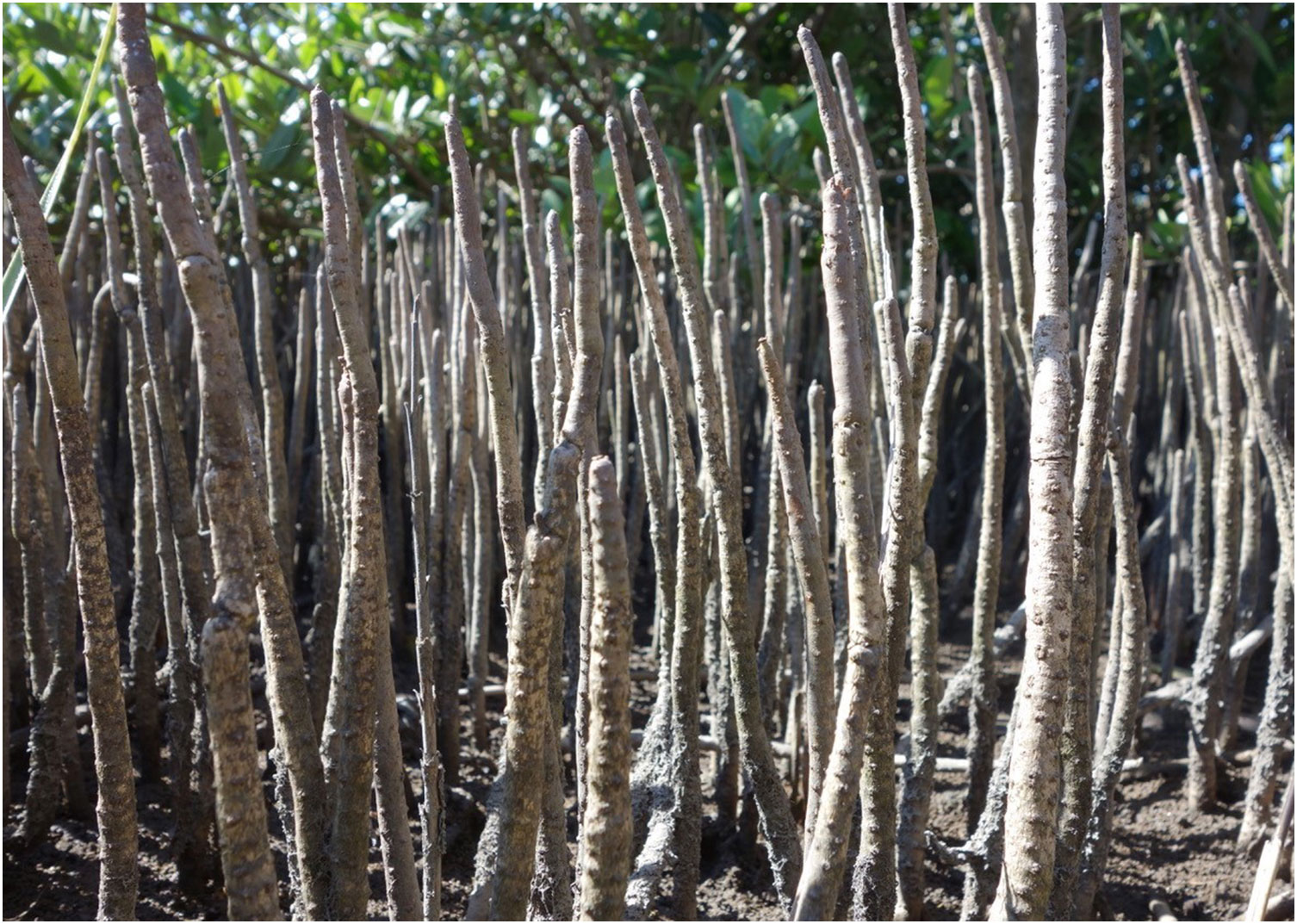
Figure 1 Black mangrove (Avicennia germinans) pneumatophores with mean diameter 1.0 ± 0.2 cm.

The rate of net deposition $(\frac{dm}{dt})$ can be described in terms of a deposition probability,

$\begin{array}{ll}\begin{array}{c}\frac{dm}{dt}=p{w}_{s}C\end{array}& (1)\end{array}$

in which $m$ is the net mass deposited per bed area over time $t$ , $p$ is the probability that particles reaching the bed will remain deposited, $w_s$ is the settling velocity, and $C$ is the near-bed suspended sediment concentration in a vertically mixed system. In Equation 1, the probability $p$ captures the influence of resuspension on mass accumulation. In the absence of resuspension, there is pure deposition ($p=1$). When resuspension is present, $p<1$. Engelund and Fredsøe (1976) developed a model to predict the probability ($p\text{'}$) that a particle on the bed is put in motion by the bed shear stress, and Zong and Nepf (2010) used this to describe the probability that a particle remains at the bed, $p=1-p\text{'}$.

$\begin{array}{ll}\begin{array}{c}p=1-{\left[1+{(\frac{\beta \pi }{6(\theta -{\theta }_c)})}^4\right]}^{-\frac{1}{4}}\end{array}.& (2)\end{array}$

$\beta$ is a bed friction coefficient, which we set to $\beta =1$. $\theta$ is the dimensionless shear stress (Shields parameter),

$\begin{array}{ll}\begin{array}{c}\theta =\frac{{\tau }_b}{({\rho }_s-\rho )g{d}_s}\end{array}& (3)\end{array}$

in which ${\tau }_b$ is the bed shear stress, ${\rho }_s$ is the sediment density, $\rho$ is the water density, $g$ is the gravitational acceleration, and $d_s$ is the particle diameter. The Shields parameter is a ratio of destabilizing (time-mean stress) and stabilizing (grain weight) forces acting on a single grain. The critical Shields parameter (${\theta }_c$) is defined by the critical bed shear stress $({\tau }_{b,c})$ needed to initiate sediment motion. When $\theta <{\theta }_c$, $p=1$, indicating pure deposition. When, θ ≤ θ_c  $p<1$, indicating the presence of resuspension.

In vegetated systems, vegetation-generated turbulence enhances resuspension by two means: (1) mixing momentum toward the bed, which enhances ${\tau }_b$ (Liu et al., 2008; Conde-Frias et al., 2023) and (2) directly interacting with the bed and mobilizing sediment with enhanced instantaneous shear and normal stress (e.g., Xu et al., 2022b). Many previous studies have described the importance of instantaneous forces (both lift and stress) associated with turbulence in mobilizing sediment grains (e.g., Bagnold, 1941; Nino and Garcia, 1996; Zanke, 2003; Smart and Habersack, 2007; Diplas et al., 2008). Sediment transport models written in terms of bed shear stress (Equation 2) have yielded inaccurate predictions for vegetated systems, because they do not account for vegetation-generated turbulence (Yang et al., 2016; Tinoco and Coco, 2018; Yang and Nepf, 2018; Liu et al., 2022). Yang et al. (2016) and Tinoco and Coco (2018) found that near-bed TKE $(k_{t(\text{nb})})$ is a better predictor of sediment motion in vegetated systems. Therefore, we hypothesized that Equation 2 might better predict deposition in vegetated systems if it were recast in terms of $(k_{t(\text{nb})})$,

$\begin{array}{ll}\begin{array}{c}p=1-{\left[1+{\left(\frac{\pi }{6({\theta }_{k_t}-{\theta }_{k_{t,c} })}\right)}^4\right]}^{-\frac{1}{4}}\end{array}.& (4)\end{array}$

In bare channels, near-bed TKE is generated by the bed shear, such that bed shear stress and TKE are linearly related (${\tau }_b=\rho \omega k_{t(\text{nb})},$ with $\omega =0.2$ , Soulsby, 1981). This relation suggests a method for redefining the critical Shields parameter (Equation 3) in terms of TKE,

$\begin{array}{ll}\begin{array}{c}{\theta }_{k_t }=\frac{\rho \omega k_{t(\text{nb})}}{({\rho }_s-\rho )g{d}_s}\end{array}& (5)\end{array}$

with ${\theta }_{k_{t,c}}$ defined by the critical near-bed TKE $(k_{t,c})$ needed to initiate sediment resuspension (Zhao and Nepf, 2021; Liu et al., 2022). Rewriting the Shields parameter in terms of TKE respects the original physical meaning, but expands the understanding of the destabilizing forces to include the effects of turbulence (e.g., Tinoco and Coco, 2018). Because the critical level of turbulence is the same in vegetated and bare channels (Yang et al., 2016), the critical turbulence level can be inferred from bare bed conditions. Specifically, $k_{t,c}={\tau }_{b,c}/\rho \omega$, such that ${\theta }_{k_{t,c}}={\theta }_c$.

Liu et al. (2022) used Equation 4 to predict deposition within a model canopy of Phragmites australis, which has a morphology consisting of a central stem surrounded by multiple leaves. Good agreement was achieved in Case 4 (Figure 8 in Liu et al., 2022), but agreement was not as good for other cases (Figure 5 in Liu et al., 2022). The robustness of the deposition model was not discussed in a systematic way across flow conditions. Further, no bare bed conditions were examined. In contrast, the present study systematically considered paired vegetated and bare bed conditions across the same range of velocity, and also extended to higher values of solid volume fraction. This facilitated a more detailed description of the parameter range over which the model may be successfully applied. Advancing existing deposition models will help to improve the modeling of sediment transport in mangrove systems and facilitate the assessment of sediment and carbon retention.

2 Materials and methods

Experiments were conducted in a recirculating Plexiglas flume with a 283 cm x 20 cm x 39 cm working section (dashed black outline in Figure 2). Plexiglas inserts (gray in Figure 2) were used to constrict the test section width to 20 cm. The water depth measured at the downstream end of the test section was $H=10 \text{cm}$, which is within depth ranges typically observed in mangrove forests (Furukawa and Wolanski, 1996; Norris et al., 2021). A sharp-crested weir ($h=5 \text{cm}$) located at the downstream end of the flume was used to fix the water depth.

FIGURE 2

Figure 2 Top view of channel. Plexiglass inserts (gray shading) constricted the test section to 20-cm width. Deposition was measured on the baseboards shown with a red outline.

Rigid vegetation, like pneumatophores, has been modeled using cylindrical dowels in several laboratory studies (Zong and Nepf, 2010; Yang et al., 2016; Tinoco and Coco, 2018; Liu et al., 2021). In this study, 0.8-cm diameter ($d$) PVC dowels were used to represent pneumatophores. The dowels were screwed into a PVC board that was inverted and inserted downward into the channel until the dowels just touched the bed. This allowed the dowels to be easily removed at the end of the experiment without disturbing the deposited sediment (Figure 2). In the field, pneumatophore canopies are spatially heterogeneous, and the pneumatophores vary in diameter (0.5 to 2 cm), height (1 to 30 cm), and solid volume fraction ($\varphi =\frac{\pi }{4}n{d}^2=$ 0.005 to 0.04, in which $n$ is roots per bed area) (Tomlinson, 2016; Yando et al., 2016; Norris et al., 2017; Norris et al., 2021). Three solid volume fractions were considered in this study: $\varphi =$ 0.01, 0.02, and 0.04. The positions of the dowels within the dowel array boards were determined using a random array generator code (MATLAB).

To characterize the flow field, a Nortek Vectrino recorded instantaneous velocity components in the streamwise ($u(t)$), lateral ($v(t)$), and vertical ($w(t)$) directions in both the bare and vegetated test sections. Four channel-averaged velocities ($U_o$) were considered (Table 1). These velocities spanned a typical range of flow conditions observed within mangrove forests (Furukawa and Wolanski, 1996; Norris et al., 2021). Velocity was measured at multiple locations across the flume at $z=$ 0.5 cm (near-bed) elevation for each channel-averaged velocity. Due to the short length of the flume, the flow was not fully developed in the bare test section, so that both wall- and bed-boundary layers were small compared to the flume width and depth. However, due to the channel constriction (Figure 2), the velocity changed 10 to 20% across the bare test-section width. This variation was captured by a five-point lateral profile in the bare section. Within the dowel array, the velocity varied at the scale of the dowel, but the laterally-averaged conditions were fully developed after just a few cylinder rows. To capture the spatial heterogeneity in the dowel array, the lateral profile included 15 positions. At each position, the velocity was measured at 200 Hz for 60 s. Tests with longer records confirmed that 60 s was sufficient to capture the mean and turbulent velocity statistics.

TABLE 1

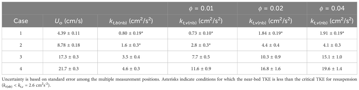
Table 1 Measured velocity and turbulent kinetic energy.

To estimate depth-averaged velocity, a profile was constructed from measurements at 0.5-cm increments from $z=$ 0.5 to 4.5 cm at a lateral position that was closest to the laterally averaged near-bed velocity. The vertical profile in the bare test section was used to calculate $U_o$. Each velocity record was decomposed into time-averaged $(\overline{u},\overline{v},\overline{w})$ and fluctuating $(u^{\prime }(t),v^{\prime }(t), w^{\prime }(t))$ components and processed using the Goring and Nikora (2002) method to remove spikes. The acceleration and velocity variance threshold parameters for this method were set to $\lambda =1$ and $k=1.5$, respectively. Turbulent kinetic energy per fluid mass is $k_t=\frac{1}{2}(\overline{u^{\text{'}2}}+ \overline{v^{\text{'}2}}+ \overline{w^{\text{'}2}})$. Near-bed laterally averaged TKE was calculated for the bare $(k_{t,b(\text{nb})})$ and vegetated $(k_{t,v(\text{nb})})$ test sections using measurements at $z=$ 0.5 cm (Table 1). Velocity measurements were made separately from the deposition experiments to avoid disturbances to the water column that could impact deposition.

The experiments used solid glass spheres with diameter $d_s=11 \text{μm}$ and density ${\rho }_s=$ 2500 kg/m³, which were selected based on grain size measured at field sites in a black mangrove forest ($\text{O}(10\text{μm})$¹). Deposition experiments began by weighing 16.3 g of glass spheres, adding them to a 1 L container with water and surfactant (Windex^® Original Glass Cleaner was added to help the sediment slurry mix with the water), and shaking the container vigorously. This mass of glass spheres was chosen to achieve an initial concentration of $C\approx 20$ mg/L throughout the flume, which is within the range of suspended sediment concentrations observed in mangrove forests (Furukawa et al., 1997; Horstman et al., 2017). The non-cohesive sediment mixture was poured across the width of the tail tank, and the recirculating pump mixed the sediment and water into a uniform concentration. Each deposition experiment ran for 4 hrs. The methodology for these deposition experiments was adapted from Zong and Nepf (2010) and Liu et al. (2022).

An optical backscatter sensor (OBS, Seapoint Sensors, Inc.) was used to measure the evolution of $C$ over the duration of the experiment (Supplementary Section 1). The OBS (20 Hz sampling rate) was located at the upstream end of the first bare baseboard and positioned at mid-depth. Preliminary studies confirmed that throughout an experiment $C$ was the same at the upstream and downstream end of the flume, so only one OBS was needed to measure $C$. This reflected the fact that the time-scale over which deposition occurred (hours) was much longer than the time-scale of mixing (minutes), with complete mixing occurring each time water passed through the pumps. Therefore, the concentration remained uniform in the test section, even as it declined due to deposition. The OBS output voltage was calibrated using prepared concentrations ranging from 0 to 44 mg/L (Supplementary Section 2).

After 4 hrs, the flume was left to slowly drain for 1 hr. Using the methodology discussed in Zhang et al. (2020), we found that the flume draining period had a negligible impact on the deposition pattern, and negligible additional deposition occurred during this time, consistent with the low $C$ at the end of the experiment. The baseboards were left to dry in the flume for 1 day. Once the baseboards were dry, the dowels were carefully lifted off the baseboards, and the bare and vegetated test section baseboards (red outline in Figure 2) were carefully removed from the flume with gloves. An acetate template was placed over each board and secured with clips. This template divided the board into three 15 cm x 15 cm windows.

Three glass fiber filters (0.7-μm pore size, 47-mm diameter) were weighed in advance, lightly wet with water, and then used to wipe the sediment off the baseboard within each window (9 filters total). Tests with additional filters indicated that using three filters was sufficient. Adding a fourth filter increased the mass by only 6%. The filters were dried in a ${60}^{\text{o}}\text{C}$ oven for 4 hrs, which was sufficient for the filters to reach a constant weight. After drying, the filters were reweighed, and the average net deposition per bed area for the bare ($m_{\text{bare}}$) and vegetated ($m_{\text{veg}}$) test sections was calculated. The uncertainty in mass deposition predominantly came from the variation among the three windows of each test section.

The deposition probability was estimated by rearranging and integrating Equation 1 over the experiment duration, $T$,

$\begin{array}{ll}p=\frac{m}{w_s{\int }_0^{T}Cdt}.& (6)\end{array}$

Using Equation 6, the deposition probability in the bare ($p_{\text{bare}}$) and vegetated ($p_{\text{veg}}$) test sections were estimated using the mass deposited in each section, $m_{\text{bare}}$and $m_{\text{veg}}$, respectively. Based on Equation 1, $C(t)$should follow an exponential decay with rate constant $-p{w}_s$. So, it was reasonable to smooth the concentration record by fitting the form $C=C_o{e}^{-bt}$with initial concentration $C_o$ and constant $b$. Because the flume was a closed system, the temporal change in $C$ was due only to deposition. The fitted concentration record was used in Equation 6 (Supplementary Section 3).

The bed shear stress in the vegetated region $({\tau }_{b,v})$ was estimated using Equation 7, developed by Conde-Frias et al. (2023), that describes the enhancement of bed shear stress by turbulence generated from rigid, emergent vegetation,

$\begin{array}{ll}\begin{array}{c}{\tau }_{b,v}=\rho {\left(\max \left(K\sqrt{\frac{k_{t,v\left(\text{nb}\right)}}{R{e}_d}}, \sqrt{C_f}{U}_o\right)\right)}^2\end{array}& (7)\end{array}$

in which $K=9.5\pm 0.4$ is a scale constant. $R{e}_d=\frac{U_{o}d}{\nu (1-\varphi )}$ is the stem Reynolds number, in which $\nu$ is the kinematic viscosity of water. $C_f=0.002$ is the bed friction coefficient (Supplementary Section 4). In the bare test section, ${\tau }_b=\rho C_f{U}_o^2$ was used to estimate bed shear stress. Conde-Frias et al. (2023) validated Equation 7 against data and simulations with $\varphi =0.016 \text{to }0.25$ and $R{e}_p$ up to 1300 (Table 2 in Conde-Frias et al. (2023)), which spans similar conditions examined in this study. Uncertainty was propagated for all calculations using the constant odds combination method described in Kline and McClintock (1953).

The critical Shields parameter was used to estimate the critical bed shear stress and critical turbulence threshold for resuspension (Zhao and Nepf, 2021). From Julien (2010),

$\begin{array}{ll}\begin{array}{c}{\theta }_c=0.25d_{*}^{-0.6}\tan ({\varphi }_R)=0.32\end{array}& (8)\end{array}$

in which ${\varphi }_R$ is the angle of repose. For the $d_s$ used in this study, ${\varphi }_R$ is ${30}^{\text{o}}$. $d_{*}$ is the dimensionless particle diameter,

$\begin{array}{ll}\begin{array}{c}{d}_{*}={\left(\frac{({\rho }_s-\rho )g}{\rho {\nu }^2}\right)}^{\frac{1}{3}}{d}_s\end{array}.& (9)\end{array}$

Equation 8 applies for $d_{*}=0.3 \text{to }1.9$. Using the parameters from this study, the critical bed shear stress and critical near-bed TKE were

$\begin{array}{ll}\begin{array}{c}{\tau }_{b,c}={\theta }_c({\rho }_s-\rho )g{d}_s=0.52\frac{\text{g}}{\text{cm}·{\text{s}}^2},\end{array}& (10)\end{array}$

$\begin{array}{ll}\begin{array}{c}{k}_{t,c}=\frac{{\tau }_{b,c}}{\rho \omega }=2.6\frac{{\text{cm}}^2}{{\text{s}}^2}\end{array}.& (11)\end{array}$

In the bare test section, $k_{t,b(\text{nb})}<k_{t,c}$ (and ${\tau }_b< {\tau }_{b,c}$) for the lower velocity Cases 1 and 2 (Table 1). Therefore, the bare test section was considered to be purely depositional $(p=1)$for these cases, from which Equation 6 can be used to estimate the settling velocity, $\overline{w_s}=$ 0.0038 $\pm$0.0003 cm/s. This was consistent with Zong and Nepf (2010), who found $w_s=$ 0.004 $\pm$ 0.002 cm/s for solid glass spheres from the same manufacturer and of the same $d$ and ${\rho }_s$ as used in this study. The estimated settling velocity was in reasonable agreement with Stokes’ Law (Stokes, 1851), $w_s=\frac{g\left(\frac{{\rho }_s}{\rho }-1\right)d_s^2}{18\nu }=$ 0.010 cm/s, given that the manufacturer’s specifications included a range of diameters (10% finer: $d_s=$ 3 μm; 90% finer: 15 μm). Using Stokes’ Law, $\overline{w_s}=$ 0.0038 cm/s suggested a mean diameter of $d_s$ = 7 μm. The value of $\overline{w_s}$ estimated from Case 1 and 2 bare test section data was subsequently used in Equation 6 to solve for the deposition probability $p$ in all other cases.

3 Results

For the same channel-averaged velocity, the vegetated test section had elevated TKE compared to the bare test section (Figure 3A). As TKE increased, resuspension increased, which was reflected in lower net deposition in the vegetated test section relative to the bare test section at the same channel-averaged velocity (Figure 3B). At the lowest velocity, all three vegetation densities produced $m_{\text{veg}}/m_{\text{bare}}$ = 1 (Figure 3B). This was also observed for $\varphi =0.01$ at the second velocity setting. For each of these cases, the near-bed turbulence was, within uncertainty, less than or equal to $k_{t,c}$ = $2.6{\text{cm}}^2/{\text{s}}^2$ (marked with asterisks in Table 1), confirming the predicted value of $k_{t,c}$ (Equation 11).

FIGURE 3

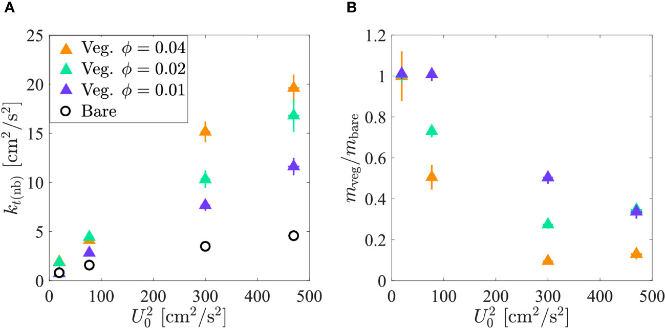
Figure 3 (A) Near-bed TKE in the bare (open black circles) and vegetated (triangles: $\varphi =$ 0.01 (purple), $\varphi =$ 0.02 (green), $\varphi =$ 0.04 (orange)) test sections versus channel-averaged velocity squared. (B) Net deposition in the vegetated test section $(m_{\text{veg}})$ normalized by net deposition in the bare test section $(m_{\text{bare}})$ versus channel-averaged velocity squared. At the lowest velocity, the three vegetated test section cases overlap. Standard error is shown by horizontal and vertical bars. In some instances, the error bars are contained within the size of the symbol. $m_{\text{veg}}$ and $m_{\text{bare}}$ data can be found in Supplementary Section 3.

For both vegetated and bare test conditions, when $k_{t(\text{nb})}\le k_{t,c}=$ 2.6 cm²/s², the deposition probability ($p$) (Equation 6) was 1 within uncertainty, and when $k_{t(\text{nb})}> k_{t,c}=$ 2.6 cm²/s², $p$ decreased with increasing $k_{t(\text{nb})}$ (Figure 4A). Furthermore, test cases with bare beds (open circles) and arrays of different solid volume fractions (triangles) collapsed to the same trend when plotted versus $k_{t(\text{nb})}$, consistent with the TKE adaptation of the Engelund and Fredsøe (1976) model (Equation 4, dashed black line in Figure 4A). In contrast, although $p$ generally decreased with increasing ${\tau }_b$, the trends were different between bare bed and vegetated conditions (Figure 4B). In the bare test section, the ${\tau }_b$ model (Equation 2, solid black line in Figure 4B) predicted a $p$ value consistent with measurements (open circles). However, in the vegetated test section, the ${\tau }_b$ model (Equation 2 with ${\tau }_{b,v}$ predicted by Equation 7) overpredicted $p$ by as much as 6-fold, because it failed to fully account for the impact of the vegetation-generated turbulence. The TKE model did best for low $k_{t(\text{nb})}$ but underpredicted $p$ for high $k_{t(\text{nb})}$ (Figure 4A).

FIGURE 4

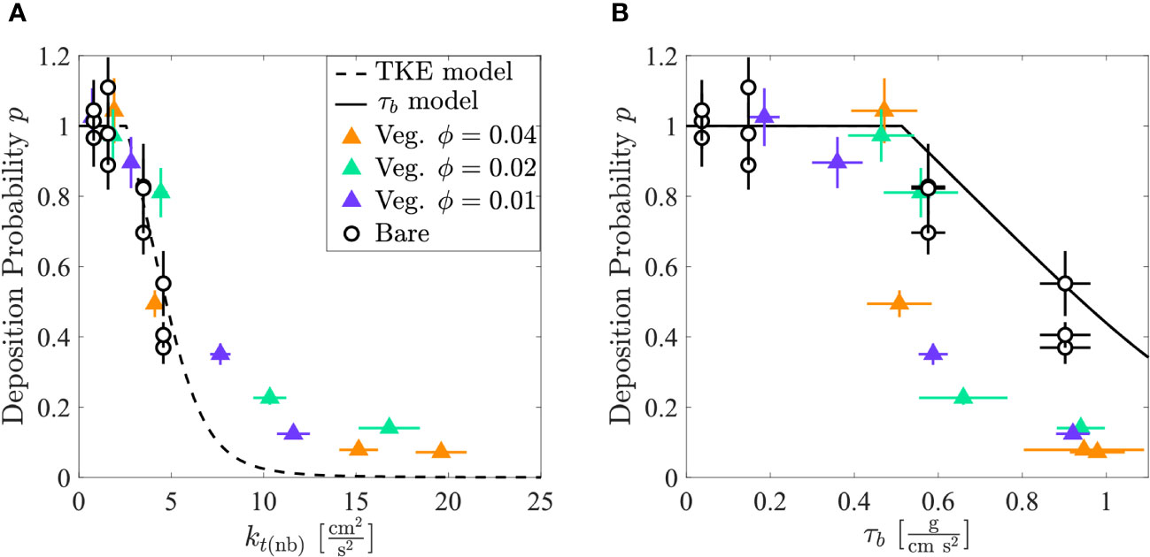
Figure 4 (A) Deposition probability in the bare (open black circles) and vegetated (triangles: $\varphi =$ 0.01 (purple), $\varphi =$ 0.02 (green), and $\varphi =$ 0.04 (orange)) test sections versus TKE. The TKE model is the dashed black line. (B) Deposition probability versus ${\tau }_b$ . The ${\tau }_b$ model is the solid black line. Standard error is shown by horizontal and vertical bars. In some instances, the error bars are contained within the size of the symbol. $p$ data can be found in Supplementary Section 3.

4 Discussion

4.1 Deposition probability within submerged vegetation

Zhang et al. (2020) measured deposition in a submerged canopy, and this data was used to estimate deposition probability, which provided a test of Equation 4 within a submerged canopy. Zhang et al. (2020) reported six cases, each with a unique velocity and stem density combination, but all with canopy height $h$ = 7.0 cm and water depth $H$ = 36 cm for Cases 1 to 5 (for Case 6 $H=$ 26 cm). Zhang et al. (2020) used solid glass spheres similar in size to those used in our experiments ($d_s$ = 7 μm, ${\rho }_s=$ 2500 kg/m³), for which the critical TKE is $k_{t,c}$ = 2.14 cm²/s² (Equation 11). The methodology for extracting the deposition probability, $p$, from the reported concentration and net deposition measurements is presented in Supplementary Section 5. The calculated deposition probability, $p$, exhibited good agreement with the TKE model (Equation 4, dashed black line in Figure 5). Additionally, the deposition probability in the bare (open circles) and vegetated (triangles) regions collapsed to the same trend when plotted versus $k_{t(\text{nb})}$.

FIGURE 5

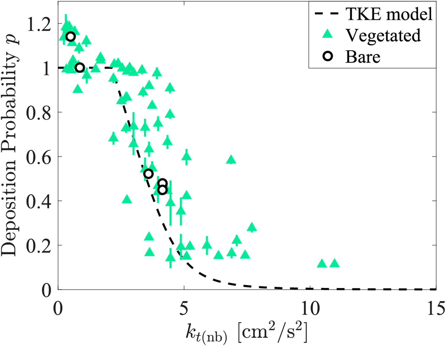
Figure 5 Deposition probability, $p$, in the bare (open black circles) and vegetated (green triangles) regions versus TKE using data from Zhang et al. (2020). The TKE model (dashed black line) was also plotted. Standard error is shown by vertical bars. In some instances, the error bars are contained within the size of the symbol.

Combining the data from Zhang et al. (2020) with the present study (Figure 4), Equation 4 has been shown to apply for bare bed, submerged, and emergent conditions. It is interesting to note that these scenarios have different turbulent length-scales. In an emergent canopy, turbulence is generated by individual roots and has a length-scale comparable to the root diameter (e.g., Tanino and Nepf, 2008). In contrast, for a submerged canopy, turbulence is generated both at the scale of individual roots and at the scale of the canopy shear layer, and both scales exist within the canopy (e.g., Poggi et al., 2004; Ghisalberti and Nepf, 2006). In the bare channel, turbulence length-scales are set by the channel depth (e.g., Nezu and Rodi, 1986). The validation of Equation 4 for all three flow scenarios, suggests that deposition probability is primarily determined by turbulence magnitude, with little dependence on turbulence scale. Possible explanations for this are discussed below.

Measurements reported in Poggi et al. (2004) show that within the lower part of a submerged canopy the turbulence length-scale is typically the cylinder diameter, and this has also been observed by T. Zhao (2023, unpublished data). Thus, between submerged and emergent canopies, the turbulence length-scales are similar near the bed, which is likely more relevant to deposition. However, this does not explain the consistency between bare bed and vegetated conditions. The lack of dependence on turbulence scale may be explained through two ideas. First, previous studies have made a similar observation for bed-load transport. Specifically, bedload transport within an emergent dowel array was observed to be dependent on the magnitude of turbulent kinetic energy (TKE), with no dependence on turbulence length-scale (Zhao and Nepf, 2021). This was explained using the impulse model for sediment entrainment, by showing that the total impulse was a function of turbulence intensity, but not eddy size. Second, very close to the bed, and specifically closer than the stem diameter, the turbulence becomes constrained in size by the proximity to the bed. For grains in this very near-bed region, the scale of the turbulence at its source (stem or shear layer) may be unimportant, so that again only turbulence magnitude is important in determining deposition probability. Further studies are needed to determine which description is correct.

4.2 Limits of deposition model

The model for deposition probability based on TKE collapsed bare and vegetated conditions better than the model based on bed shear stress. However, for both emergent and submerged vegetation, the TKE model underpredicted deposition for the highest turbulence intensities, specifically for $k_{t(\text{nb})}$ > 5 cm²/s² (Figures 4, 5). A similar underprediction of measured deposition was observed in Figure 8 of Liu et al. (2022), but for $k_{t(\text{nb})}$ > 15 cm²/s². The higher turbulence threshold might be a function of sediment size, as Liu et al. (2022) considered a larger particle (22 µm), compared to the present study (11 µm). The underprediction at high TKE may be related to the spatial heterogeneity of vegetated flows. The presence of vegetation creates preferential flow patterns that channel higher velocity through more open regions and create some lower velocity regions such as in the lee of stems. The zones of lower velocity and lower TKE may allow for greater deposition than predicted from Equation 4 using the spatially-averaged TKE. In the cases considered here, the deviations of the TKE model occur for $k_{t(\text{nb})}$ greater than 5 cm²/s² and p less than 0.2 to 0.3. None of the bare section cases considered here had $k_{t(\text{nb})}$ high enough or p low enough to evaluate the applicability of the TKE model in that range. Additional measurements in this part of the parameter space could improve the TKE-based deposition probability for both vegetated and unvegetated flow conditions.

4.3 Exploration of field conditions

Vegetation generates drag that reduces the mean flow, which limits the horizontal transport of sediment and promotes deposition. The tendency toward enhanced deposition within vegetated regions may be modified by root-generated turbulence, which can reduce deposition probability and extend the distance sediment travels from a source region before it deposits. To explore the role of root-generated turbulence in sediment retention within a mangrove forest, field conditions were used to evaluate the trends in velocity and deposition probability across a range of typical root density, and these were used to evaluate the time and spatial scales of deposition within the forest. Consider the inundation of a mangrove forest from an ocean edge or channel edge. The velocity entering the mangrove platform depends on the water surface slope, $S$, set up by an advancing tide. Assuming the pneumatophores are emergent, conservation of momentum predicts the velocity entering the root layer (e.g., Xu et al., 2022a),

$\begin{array}{ll}\begin{array}{c}U= \sqrt{\frac{gHS}{C_f+0.5C_{d}ndH}}\end{array}& (12)\end{array}$

in which $C_d$ is the root drag coefficient, $C_f$ is the bed friction coefficient, and $n$ is the root density. To apply the TKE model to describe the deposition probability $p$, the TKE within the pneumatophore layer was estimated as the sum of bed-generated and root-generated turbulence (Yang et al., 2016),

$\begin{array}{ll}{k}_{t,v(\text{nb})}=\underset{k_{t(\text{bed})}}{\underbrace{\frac{{\tau }_b}{\rho \omega }}}+\underset{k_{t(\text{root})}}{\underbrace{{{\delta }_{k_t}\left(\frac{C_{d,\text{form}} n{d}^2}{2(1-\varphi )}\right)}^{\frac{2}{3}}{U}^2}}& (13)\end{array}$

in which ${\delta }_{k_t}$ is a scale constant, and $C_{d,\text{form}}$ is the form drag coefficient for the cylindrical root. Zhao and Nepf (2021) found ${\delta }_{k_t}=0.52\pm 0.07$ based on data over a four-fold variation in stem diameter (0.64 to 2.5 cm). For $R{e}_d\ge 200$, Etminan et al. (2018) found $C_{d,\text{form}}=0.9C_d$. Based on Etminan et al. (2017), $C_d=1$ is a reasonable approximation, in which $C_d$ is the sum of form drag and viscous drag. Equation 13 assumes vegetation-generated turbulence is present, which requires $R{e}_d > 120$ (Liu and Nepf, 2016). Equation 7 requires a priori knowledge of $k_{t,v(\text{nb})}$. To avoid iterative calculations, ${\tau }_b$ in Equation 13 was predicted with the following model from Yang and Nepf (2018),

$\begin{array}{ll}\begin{array}{c}{\tau }_b= \{\begin{array}{c}\frac{4\rho \nu U_0}{d}, R{e}_d<\frac{4}{C_f}\\ \rho C_f{U}_0^2, R{e}_d\ge \frac{4}{C_f}.\end{array}\end{array}& (14)\end{array}$

Using the predicted TKE, the deposition probability was estimated using the TKE model (Equation 4). For comparison, deposition probability was also estimated using the ${\tau }_b$ model (Equation 2), with the bed shear stress predicted using Equation 7. This comparison was used to illustrate the influence of root-generated turbulence on the time and length scales that describe deposition.

For a tidal cycle of duration $T$, we can simplify the transport into a period of a positive velocity $U$ flooding the forest, followed by a negative $U$ draining the forest. On average, water remains in the forest for a residence time $T_R=T/2$. The fraction of sediment entering the forest that is deposited and retained can be estimated by comparing the residence time to the time scale for deposition. Consistent with Equation 1, deposition is modeled as a first-order reaction, $\partial C/\partial t=-\left(\frac{p{w}_s}{H}\right)C$, which indicates the settling time scale,

$\begin{array}{ll}\begin{array}{c}{T}_{settle }=\frac{H}{p{w}_s}\end{array}& (15)\end{array}$

Further, deposition near the channel or ocean edge reduces the sediment supplied to regions farther from the edge, which results in net deposition that decays away from the edge over an e-folding length-scale (e.g., Equation 2 in Furukawa and Wolanski, 1996),

$\begin{array}{ll}\begin{array}{c}{L}_{dep}=T_{settle}U\end{array}.& (16)\end{array}$

Equations 2, 4, 7, 12, 13, 14, 15, and 16 were used to estimate $U$, $p$, $T_{settle}/T_R$ and $L_{dep}$ as a function of root density (Figure 6). Physical parameters were chosen based on representative field conditions: tidal cycle of $T=$ 12 hours, water depth $H=$ 20 cm, for which pneumatophores should be emergent, root diameter $d =$ 0.8 cm, and root density $n$ = 0 to 800 roots $/{\text{m}}^2$, which corresponds to $\varphi \approx 0$ to 0.04. To achieve velocities within typical ranges observed in mangrove forests (0 to 0.2 m/s, Furukawa and Wolanski, 1996; Norris et al., 2021), the water surface slope was set to $S=$ 0.001 (Mullarney et al., 2017b). The settling velocity was set to $w_s=0.05$ cm/s, which is within the typical range of settling velocities measured for flocs with $d_s=O(10) \text{μm}$ (Gibbs, 1985). The bed friction coefficient was set to $C_f =$ 0.002. Note that this analysis ignores spatial and temporal variability in tidal velocity, water depth, and sediment characteristics that would be present in natural systems but are beyond the scope of a simplified scale analysis.

FIGURE 6

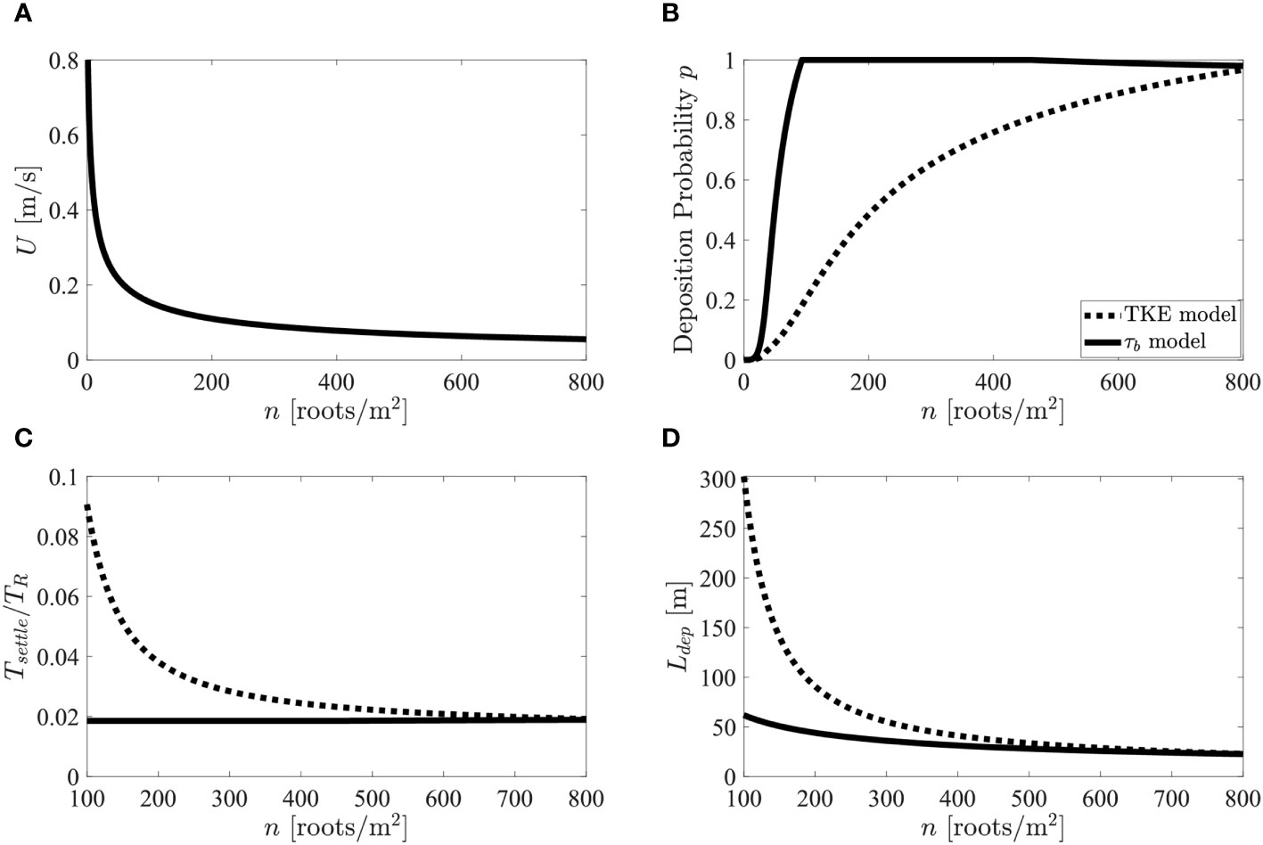
Figure 6 (A) Velocity in mangrove root layer versus root density. (B) Deposition probability versus root density. (C) Ratio of settling time to residence time versus root density. (D) Deposition length-scale. ${\tau }_b$ model (solid black line) and TKE model (dashed black line) in Figures 7B–D.

As $n$ increased, $U$ decreased (Figure 6A), resulting in a decrease in both TKE (Equation 13) and ${\tau }_b$ (Equation 7), both of which increased $p$ (Figure 6B). Thus, the strong reduction in velocity due to vegetation drag makes regions of vegetation more conducive to deposition compared to bare regions. Including the influence of root-generated turbulence (dashed line, Figure 6B) produced lower values of $p$ over the entire range of root density when compared to the ${\tau }_b$ model (solid line, Figure 6B), which did not reflect the influence of root-generated turbulence. The lower values of $p$ associated with root-generated turbulence kept sediment in suspension longer (i.e., TKE model produced longer $T_{settle}$, Figure 6C). However, the longer settling time did not influence the ability of the forest to capture the sediment, since $T_{settle}/T_R$<< 1 across the range of root density associated with mangrove forests ($n$ > 100 roots/m², Figure 6C), suggesting that a typical mangrove forest captures the majority of sediment carried in by tidal flux. However, root-generated turbulence did impact the distance into the forest that sediment can be supplied, $L_{dep}$, with root-turbulence enhancing $L_{dep}$ by up to a factor of five (Figure 6D).

To conclude, root-generated turbulence enhanced resuspension and diminished the rate of net deposition. Specifically, for the same velocity, as root density increased, TKE increased and net deposition decreased. The influence of root-generated turbulence can be described in terms of a deposition probability ($p$), which was predicted from a modified version of Engelund and Fredsøe’s (1976) model written in terms of near-bed TKE. For the range of root densities found in mangrove forests, the model suggested that root-generated turbulence did not change the amount of sediment captured during a tidal cycle but greatly increased the distance over which the captured sediment was deposited within the forest.

Data availability statement

The original contributions presented in the study are included in the article/Supplementary Material. Further inquiries can be directed to the corresponding author.

Author contributions

AD: Conceptualization, Data curation, Formal Analysis, Investigation, Methodology, Visualization, Writing – original draft, Writing – review & editing. EH: Formal Analysis, Investigation, Writing – review & editing. DR: Conceptualization, Formal Analysis, Supervision, Writing – original draft, Writing – review & editing. HN: Conceptualization, Formal Analysis, Funding acquisition, Methodology, Project administration, Resources, Supervision, Writing – original draft, Writing – review & editing.

Funding

The author(s) declare financial support was received for the research, authorship, and/or publication of this article. This study was supported by Shell International Exploration and Production through the MIT Energy Initiative. AD was supported in part by the National Science Foundation Graduate Research Fellowship under Grant No. 2141064.

Acknowledgments

We would like to thank Stephen Rudolph for his help with designing and constructing the flume inserts that made this research possible.

Conflict of interest

The authors declare that the research was conducted in the absence of any commercial or financial relationships that could be construed as a potential conflict of interest.

Publisher’s note

All claims expressed in this article are solely those of the authors and do not necessarily represent those of their affiliated organizations, or those of the publisher, the editors and the reviewers. Any product that may be evaluated in this article, or claim that may be made by its manufacturer, is not guaranteed or endorsed by the publisher.

Supplementary material

The Supplementary Material for this article can be found online at: https://www.frontiersin.org/articles/10.3389/fmars.2023.1266241/full#supplementary-material

Footnotes

1. ^ Deitrick, A. R., Ralston, D. K., Baustian, M. M., Esposito, C. R., Beltrán-Burgos, M., Courtois, A. J., et al. (2023) Cohesive sediment erosion within mangrove pneumatophores, Submitted.

References

Adame M. F., Lovelock C. E. (2011). Carbon and nutrient exchange of mangrove forests with the coastal ocean. Hydrobiologia 663 (1), 23–50. doi: 10.1007/s10750-010-0554-7

CrossRef Full Text | Google Scholar

Alongi D. M. (2014). Carbon cycling and storage in mangrove forests. Annu. Rev. Mar. Sci. 6 (1), 195–219. doi: 10.1146/annurev-marine-010213-135020

CrossRef Full Text | Google Scholar

Bagnold R. A. (1941). The physics of blown sand and desert dunes (London, Methuen: Courier Corporation).

Google Scholar

Barbier E. B., Hacker S. D., Kennedy C., Koch E. W., Stier A. C., Silliman B. R. (2011). The value of estuarine and coastal ecosystem services. Ecol. Monogr. 81 (2), 169–193. doi: 10.1890/10-1510.1

CrossRef Full Text | Google Scholar

Conde-Frias M., Ghisalberti M., Lowe R. J., Abdolahpour M., Etminan V. (2023). The near-bed flow structure and bed shear stresses within emergent vegetation. Water Resour. Res. 59 (4), e2022WR032499. doi: 10.1029/2022WR032499

CrossRef Full Text | Google Scholar

de Groot R., Brander L., van der Ploeg S., Costanza R., Bernard F., Braat L., et al. (2012). Global estimates of the value of ecosystems and their services in monetary units. Ecosystem Serv. 1 (1), 50–61. doi: 10.1016/j.ecoser.2012.07.005

CrossRef Full Text | Google Scholar

Diplas P., Dancey C. L., Celik A. O., Valyrakis M., Greer K., Akar T. (2008). The role of impulse on the initiation of particle movement under turbulent flow conditions. Science 322 (5902), 717–720. doi: 10.1126/science.1158954

PubMed Abstract | CrossRef Full Text | Google Scholar

Engelund F., Fredsøe J. (1976). A sediment transport model for straight alluvial channels. Hydrology Res. 7 (5), 293–306. doi: 10.2166/nh.1976.0019

CrossRef Full Text | Google Scholar

Etminan V., Ghisalberti M., Lowe R. J. (2018). Predicting bed shear stresses in vegetated channels. Water Resour. Res. 54 (11), 9187–9206. doi: 10.1029/2018WR022811

CrossRef Full Text | Google Scholar

Etminan V., Lowe R. J., Ghisalberti M. (2017). A new model for predicting the drag exerted by vegetation canopies. Water Resour. Res. 53 (4), 3179–3196. doi: 10.1002/2016WR020090

CrossRef Full Text | Google Scholar

Fagherazzi S., Bryan K. R., Nardin W. (2017). Buried alive or washed away: the challenging life of mangroves in the Mekong Delta. Oceanography 30 (3), 48–59. doi: 10.5670/oceanog.2017.313

CrossRef Full Text | Google Scholar

Furukawa K., Wolanski E. (1996). Sedimentation in mangrove forests. Mangroves Salt Marshes 1 (1), 3–10. doi: 10.1023/A:1025973426404

CrossRef Full Text | Google Scholar

Furukawa K., Wolanski E., Mueller H. (1997). Currents and sediment transport in mangrove forests. Estuarine Coast. Shelf Sci. 44 (3), 301–310. doi: 10.1006/ecss.1996.0120

CrossRef Full Text | Google Scholar

Ghisalberti M., Nepf H. (2006). The structure of the shear layer in flows over rigid and flexible canopies. Environ. Fluid Mechanics 6 (3), 277–301. doi: 10.1007/s10652-006-0002-4

CrossRef Full Text | Google Scholar

Gibbs R. J. (1985). Estuarine flocs: Their size, settling velocity and density. J. Geophysical Research: Oceans 90 (C2), 3249–3251. doi: 10.1029/JC090iC02p03249

CrossRef Full Text | Google Scholar

Goring D. G., Nikora V. I. (2002). Despiking acoustic doppler velocimeter data. J. Hydraulic Eng. 128 (1), 117–126. doi: 10.1061/(ASCE)0733-9429(2002)128:1(117

CrossRef Full Text | Google Scholar

Horstman E. M., Dohmen-Janssen C. M., Narra P. M. F., van den Berg N. J. F., Siemerink M., Hulscher S. J. M. H. (2014). Wave attenuation in mangroves: A quantitative approach to field observations. Coast. Eng. 94, 47–62. doi: 10.1016/j.coastaleng.2014.08.005

CrossRef Full Text | Google Scholar

Horstman E. M., Mullarney J. C., Bryan K. R., Sandwell D. R. (2017). “Deposition gradients across mangrove fringes,” in Coastal Dynamics 2017 Conference. 911–922. Available at: https://researchcommons.waikato.ac.nz/handle/10289/11160.

Google Scholar

Hutchison J., Spalding M., zu Ermgassen P. (2014). The role of mangroves in fisheries enhancement (The Nature Conservancy and Wetlands International).

Google Scholar

Jennerjahn T. C., Ittekkot V. (2002). Relevance of mangroves for the production and deposition of organic matter along tropical continental margins. Naturwissenschaften 89 (1), 23–30. doi: 10.1007/s00114-001-0283-x

PubMed Abstract | CrossRef Full Text | Google Scholar

Julien P. Y. (2010). Erosion and sedimentation (Cambridge: Cambridge University Press).

Google Scholar

Kauffman J. B., Adame M. F., Arifanti V. B., SChile-Beers L. M., Bernardino A. F., Bhomia R. K., et al. (2020). Total ecosystem carbon stocks of mangroves across broad global environmental and physical gradients. Ecol. Monogr. 90 (2), e01405. doi: 10.1002/ecm.1405

CrossRef Full Text | Google Scholar

Kline, McClintock (1953). The description of uncertainties in a single-sample experiment. Mechanical Eng. 75, 3–8.

Google Scholar

Liu D., Diplas P., Fairbanks J. D., Hodges C. C. (2008). An experimental study of flow through rigid vegetation. J. Geophysical Research: Earth Surface 113 (F4). doi: 10.1029/2008JF001042

CrossRef Full Text | Google Scholar

Liu C., Nepf H. (2016). Sediment deposition within and around a finite patch of model vegetation over a range of channel velocity. Water Resour. Res. 52 (1), 600–612. doi: 10.1002/2015WR018249

CrossRef Full Text | Google Scholar

Liu C., Shan Y., Nepf H. (2021). Impact of stem size on turbulence and sediment resuspension under unidirectional flow. Water Resour. Res. 57 (3), e2020WR028620. doi: 10.1029/2020WR028620

CrossRef Full Text | Google Scholar

Liu C., Yan C., Sun S., Lei J., Nepf H., Shan Y. (2022). Velocity, turbulence, and sediment deposition in a channel partially filled with a phragmites australis canopy. Water Resour. Res. 58 (8), e2022WR032381. doi: 10.1029/2022WR032381

CrossRef Full Text | Google Scholar

Mazda Y., Magi M., Ikeda Y., Kurokawa T., Asano T. (2006). Wave reduction in a mangrove forest dominated by Sonneratia sp. Wetlands Ecol. Manage. 14 (4), 365–378. doi: 10.1007/s11273-005-5388-0

CrossRef Full Text | Google Scholar

Mazda Y., Wolanski E., King B., Sase A., Ohtsuka D., Magi M. (1997). Drag force due to vegetation in mangrove swamps. Mangroves Salt Marshes 1 (3), 193–199. doi: 10.1023/A:1009949411068

CrossRef Full Text | Google Scholar

Mcleod E., Chmura G. L., Bouillon S., Salm R., Björk M., Duarte C. M., et al. (2011). A blueprint for blue carbon: Toward an improved understanding of the role of vegetated coastal habitats in sequestering CO2. Front. Ecol. Environ. 9 (10), 552–560. doi: 10.1890/110004

CrossRef Full Text | Google Scholar

Mullarney J. C., Henderson S. M., Norris B. K., Bryan K. R., Fricke A. T., Sandwell D. R., et al. (2017a). A question of scale: how turbulence around aerial roots shapes the seabed morphology in mangrove forests of the Mekong Delta. Oceanography 30 (3), 34–47. doi: 10.5670/oceanog.2017.312

CrossRef Full Text | Google Scholar

Mullarney J. C., Henderson S. M., Reyns J. A. H., Norris B. K., Bryan K. R. (2017b). Spatially varying drag within a wave-exposed mangrove forest and on the adjacent tidal flat. Continental Shelf Res. 147, 102–113. doi: 10.1016/j.csr.2017.06.019

CrossRef Full Text | Google Scholar

Nellemann C., Corcoran E., Duarte C. M., Valdés L., De Young C., Fonseca L., et al. (2009). Blue carbon. A rapid response assessment (GRID-Arendal: United Nations Environment Programme)ISBN: 978-82-7701-060-1. Available at: www.grida.no.

Google Scholar

Nezu I., Rodi W. (1986). Open-channel flow measurements with a laser doppler anemometer. J. Hydraulic Eng. 112 (5), 335–355. doi: 10.1061/(ASCE)0733-9429(1986)112:5(335

CrossRef Full Text | Google Scholar

Nino Y., Garcia M. (1996). Experiments on particle–turbulence interactions in the near–wall region of an open channel flow: Implications for sediment transport. J. Fluid Mechanics 326, 285–319. doi: 10.1017/S0022112096008324

CrossRef Full Text | Google Scholar

Norris B. K., Mullarney J. C., Bryan K. R., Henderson S. M. (2017). The effect of pneumatophore density on turbulence: A field study in a Sonneratia-dominated mangrove forest, Vietnam. Continental Shelf Res. 147, 114–127. doi: 10.1016/j.csr.2017.06.002

CrossRef Full Text | Google Scholar

Norris B. K., Mullarney J. C., Bryan K. R., Henderson S. M. (2019). Turbulence within natural mangrove pneumatophore canopies. J. Geophysical Research: Oceans 124 (4), 2263–2288. doi: 10.1029/2018JC014562

CrossRef Full Text | Google Scholar

Norris B. K., Mullarney J. C., Bryan K. R., Henderson S. M. (2021). Relating millimeter-scale turbulence to meter-scale subtidal erosion and accretion across the fringe of a coastal mangrove forest. Earth Surface Processes Landforms 46 (3), 573–592. doi: 10.1002/esp.5047

CrossRef Full Text | Google Scholar

Poggi D., Porporato A., Ridolfi L., Albertson J. D., Katul G. G. (2004). The effect of vegetation density on canopy sub-layer turbulence. Boundary-Layer Meteorology 111 (3), 565–587. doi: 10.1023/B:BOUN.0000016576.05621.73

CrossRef Full Text | Google Scholar

Smart G., Habersack H. (2007). Pressure fluctuations and gravel entrainment in rivers. J. Hydraulic Res. 45 (5), 661–673. doi: 10.1080/00221686.2007.9521802

CrossRef Full Text | Google Scholar

Soulsby R. L. (1981). Measurements of the Reynolds stress components close to a marine sand bank. Mar. Geology 42 (1), 35–47. doi: 10.1016/0025-3227(81)90157-2

CrossRef Full Text | Google Scholar

Stokes G. G. (1851). “On the effect of the internal friction of fluids on the motion of pendulums,” in Transactions of the cambridge philosophical society, part II. 9, 8–106.

Google Scholar

Tanino Y., Nepf H. M. (2008). Lateral dispersion in random cylinder arrays at high Reynolds number. J. Fluid Mechanics 600, 339–371. doi: 10.1017/S0022112008000505

CrossRef Full Text | Google Scholar

Temmink R. J. M., Lamers L. P. M., Angelini C., Bouma T. J., Fritz C., van de Koppel J., et al. (2022). Recovering wetland biogeomorphic feedbacks to restore the world’s biotic carbon hotspots. Science 376 (6593). doi: 10.1126/science.abn1479

CrossRef Full Text | Google Scholar

Tinoco R. O., Coco G. (2018). Turbulence as the main driver of resuspension in oscillatory flow through vegetation. J. Geophysical Research: Earth Surface 123 (5), 891–904. doi: 10.1002/2017JF004504

CrossRef Full Text | Google Scholar

Tomlinson P. B. (2016). The botany of mangroves (Cambridge: Cambridge University Press).

Google Scholar

Twilley R. R., Castañeda-Moya E., Rivera-Monroy V. H., Rovai A. (2017). “Productivity and carbon dynamics in mangrove wetlands,” in Mangrove ecosystems: A global biogeographic perspective. Eds. Rivera-Monroy V., Lee S., Kristensen E., Twilley R. (Cham: Springer). doi: 10.1007/978-3-319-62206-4_5

CrossRef Full Text | Google Scholar

Vo-Luong P., Massel S. (2008). Energy dissipation in non-uniform mangrove forests of arbitrary depth. J. Mar. Syst. 74 (1), 603–622. doi: 10.1016/j.jmarsys.2008.05.004

CrossRef Full Text | Google Scholar

Woodroffe C. D., Rogers K., McKee K. L., Lovelock C. E., Mendelssohn I. A., Saintilan N. (2016). Mangrove sedimentation and response to relative sea-level rise. Annu. Rev. Mar. Sci. 8 (1), 243–266. doi: 10.1146/annurev-marine-122414-034025

CrossRef Full Text | Google Scholar

Xu Y., Esposito C. R., Beltrán-Burgos M., Nepf H. M. (2022a). Competing effects of vegetation density on sedimentation in deltaic marshes. Nat. Commun. 13 (1), 1. doi: 10.1038/s41467-022-32270-8

PubMed Abstract | CrossRef Full Text | Google Scholar

Xu Y., Li D., Nepf H. (2022b). Sediment pickup rate in bare and vegetated channels. Geophysical Res. Lett. 49 (21), e2022GL101279. doi: 10.1029/2022GL101279

CrossRef Full Text | Google Scholar

Yando E. S., Osland M. J., Willis J. M., Day R. H., Krauss K. W., Hester M. W. (2016). Salt marsh-mangrove ecotones: Using structural gradients to investigate the effects of woody plant encroachment on plant–soil interactions and ecosystem carbon pools. J. Ecol. 104 (4), 1020–1031. doi: 10.1111/1365-2745.12571

CrossRef Full Text | Google Scholar

Yang J. Q., Chung H., Nepf H. M. (2016). The onset of sediment transport in vegetated channels predicted by turbulent kinetic energy. Geophysical Res. Lett. 43 (21), 11,261–11,268. doi: 10.1002/2016GL071092

CrossRef Full Text | Google Scholar

Yang J. Q., Nepf H. M. (2018). A turbulence-based bed-load transport model for bare and vegetated channels. Geophysical Res. Lett. 45 (19), 10,428–10,436. doi: 10.1029/2018GL079319

CrossRef Full Text | Google Scholar

Zanke U. (2003). On the influence of turbulence on the initiation of sediment motion. Int. J. Sediment Res. 18 (1), 17–31.

Google Scholar

Zhang J., Lei J., Huai W., Nepf H. (2020). Turbulence and particle deposition under steady flow along a submerged seagrass meadow. J. Geophysical Research: Oceans 125 (5), e2019JC015985. doi: 10.1029/2019JC015985

CrossRef Full Text | Google Scholar

Zhao T., Nepf H. M. (2021). Turbulence dictates bedload transport in vegetated channels without dependence on stem diameter and arrangement. Geophysical Res. Lett. 48 (21), e2021GL095316. doi: 10.1029/2021GL095316

CrossRef Full Text | Google Scholar

Zong L., Nepf H. (2010). Flow and deposition in and around a finite patch of vegetation. Geomorphology 116 (3), 363–372. doi: 10.1016/j.geomorph.2009.11.020

CrossRef Full Text | Google Scholar