 Cui Baolong
 Liu Jingyi
 Guo Wuhong1,2
94% of researchers rate our articles as excellent or good
Learn more about the work of our research integrity team to safeguard the quality of each article we publish.
Find out more
ORIGINAL RESEARCH article
Front. Mar. Sci. , 06 November 2023
Sec. Ocean Observation
Volume 10 - 2023 | https://doi.org/10.3389/fmars.2023.1259864
This article is part of the Research Topic Ocean Observation based on Underwater Acoustic Technology, volume II View all 23 articles
Ocean Acoustic Tomography (OAT) is an efficient and economical marine acoustic observation technique. Targeted observation is an appealing procedure to reduce the uncertainty of ocean environment prediction through additional observation. This study aimed to assess the validity of OAT as an observation method for targeted observation. OAT based on Niche Genetic Algorithm was employed to extract sound speed and temperature profiles from acoustic transmission time, utilizing data from the 2019 Yellow Sea experiment. The inversion results were compared with measurement data, which are found to be accurate and reliable. To further evaluate OAT as targeted observation method, the vertical bias structure of OAT was added on synchronous measurement data in the sensitive area of targeted observation to simulate OAT observation in sensitive area. This simulated data was then incorporated into a 3D-Var assimilation system to improve the short-term prediction of the target region. Comparing the predictions derived with the measurement data at the verification time, it shows that the simulated OAT observation improved the quality of target region prediction, indicating that OAT can be an effective observation method for targeted observation. An Observing System Simulation Experiment was conducted to assess the impact of OAT characteristics on prediction improvement. The results show that both adding observation nodes and extending the observation duration have positive effects, while extending the observation duration performs better.
Ocean acoustic tomography (OAT) is a marine remote sensing technique by utilizing the sound field generated from measured properties (Worcester, 2019). This method extracts acoustic characteristics, such as Sound Speed Profile (SSP), through the analysis of travel time or other acoustic signals. Corresponding marine environment characteristics is inverted through the ocean-acoustic coupled relationship. The concept of OAT was initially proposed by Munk and Wunsch (Munk and Wunsch, 1979; Munk et al, 1995), aiming to investigate mesoscale phenomena such as vortices, convection, and internal waves. An advantage of OAT over other methods is its ability to facilitate long-term, large-area, and cost-effective ocean monitoring, taking advantage of the characteristics that acoustic signals transmit over long distances and acoustic propagation is sensitive to the marine environment (Dushaw et al, 2001).
Numerous OAT experiments have been conducted since the 1980s, showcasing the versatility and potential of this technique. RTE83 experiment (DeFerrari and Nguyen, 1986; Howe, 1987) validated the feasibility of flow velocity inversion using a single source-receiver pair of acoustic nodes in a range-dependent environment, achieving success at a distance of 300km in Atlantic Ocean. In 1988-1989, Greenland Sea Tomography experiment (Jin et al, 1993) became the first to employ mobile nodes to estimate the effect of sea ice on acoustic pulses. SLICE89 experiment (Howe et al, 1991) combined acoustic tomography with ocean models to enable ocean forecasting on a scale of 1000-2000km. AMODE experiment (Dushaw et al, 2001) conducted in 1991 utilized mobile nodes to measure eddy currents in Northwest Atlantic. Acoustic Thermometry of Ocean Climate (ATOC) experiment, organized by International Ocean Research Association (Dushaw and Worester, 2001; Dushaw, 1999), stands out as a remarkable achievement. This experiment incorporated vertical line arrays, submarine receiving arrays, and US Army’s SOSUS system to receive low-frequency acoustic signals propagating over basin distances. Its purpose was to monitor long-term temperature changes and global warming as indicators of climate trends. In 2001, ASIAEX experiment (Duda et al, 2004), conducted in collaboration with various countries and organizations, focused on the seas surrounding China. Its primary objective was to investigate the interaction mechanism between the acoustic field and the water bodies. It is shown that the mutual correlation function and Green’s function of marine environmental noise have the similarity of arrival time structure, based on which some scholars proposed the idea of using marine environmental noise for passive acoustic tomography, and the idea was realised by experimental observation (Gasparini et al, 1997; Fried et al, 2013; Li et al, 2019). The presence of mesoscale processes such as ocean fronts/vortices in the oceans has led to the development of acoustic tomography for horizontally varying environmental (Carrière and Hermand, 2008; Yang et al, 2022);. In recent years, coastal acoustic tomography technology has made significant progress, particularly in monitoring semi-enclosed environments such as ports and bays (Yamoaka et al, 2002; Zhu et al, 2010; Zhu et al, 2013). Additionally, acoustic tomography has been applied to observe mesoscale phenomena such as internal waves (Lynch et al, 1996; Dahl et al, 2004; Li et al, 2014) and Kuroshio current (Yuan et al, 1999; Lebedev et al, 2003; Huang et al, 2013; Taniguchi et al, 2023). Currently, experimental research primarily emphasizes coastal velocity inversion, with limited studies focusing on marine environment inversion, especially in the context of oceanic environment prediction.
The essence of acoustic tomography lies in the recognition of acoustic signal propagation time and structure. Several mainstream methods are commonly used in this field, including ray travel time tomography (Munk et al, 1995), matched-peak tomography (Skarsoulis et al, 1996), modal travel time tomography (Shang, 1989), modal-phase tomography, and modal-horizontal-refraction tomography (Shang et al, 2000). Ray travel time tomography, being the most classic and widely used method, employs matching filters to measure the travel time. Matched-peak tomography locates the maximum peak value in the arrival pattern and analyzes the peak structure of the signal to determine the travel time accurately. Modal travel time tomography, on the other hand, relies on the principles of normal mode theory to identify the arrival time. Normal wave phase tomography and horizontal refraction tomography, which are similar, replace the normal wave travel time with the normal wave phase or horizontal refraction angle. These substitutions are then substituted into algorithms to obtain the desired travel time information. Regarding the acquisition algorithms of travel time, two common approaches are utilized: the perturbation method (Munk et al, 1995) and the matching field method (Taroudakis and Markaki, 1997). The perturbation method assumes that the difference between the theoretical calculation and measured propagation delays is proportional to the difference in sound velocity. However, this method tends to be less accurate in complex and non-linear marine environments. In contrast, the matching field method aims to obtain the optimal solution that corresponds to the measured values through acoustic and marine models. The effectiveness of this method relies on the accuracy of the model and the efficiency of the optimization algorithm employed.
Targeted observation, also known as adaptive observation, is a strategy approach aimed at reducing numerical prediction uncertainty through employing additional observations. In this strategy, the goal is to improve the prediction quality of a specific area, referred to as the target region, at a designated verification time. To achieve this, additional observations are deployed within sensitive areas to acquire additional information. This additional information is subsequently assimilated into the ocean model to refine Initial Conditions (ICs) and improve the prediction accuracy (Rabier et al, 1996; Rabier et al, 1996; Snyder, 1996; Mu, 2013). Originally introduced in atmospheric studies, targeted observation has undergone validation through a series of field experiments such as FASTEX (Joly et al, 1999), NOPREX (Langland et al, 1999), and WSRP (Szunyogh et al, 2000). Recognizing its potential, World Meteorological Organization (WMO) proposed The Observing System Research and Predictability Experiment (THORPEX), which integrated targeted observation concepts into a scientific framework for improving global high-impact weather prediction (Parsons et al, 2017). More recently, the concept of targeted observation has been extended to oceanic prediction studies, although the focus has primarily been on large-scale ocean phenomena, such as Indian Ocean Dipole (Feng et al, 2016) and Kuroshio (Kramer et al, 2012; Wang et al, 2013; Zhang et al, 2017). However, there remains a scarcity of researches related to the acoustic field within targeted observation studies.
The identification of sensitive areas, a crucial aspect of targeted observation, relies on two types of algorithms. The first type is based on ensemble prediction techniques, such as Ensemble Kalman Filter (EnKF) (Hamill and Snyder, 2002) and Ensemble Transform Kalman Filter (ETKF) (Bishop et al, 2001). These algorithms specifically focus on calculating the reduction in forecast error covariance resulting from different observation configurations (Wei et al, 2008; Zhang et al, 2015; Feng et al, 2019; Thiruvengadam et al, 2021). The second type of algorithm is based on adjoint mode techniques, which include approaches such as Singular Vectors (SV) (Buizza and Montani, 1999), adjoint sensitivity (Baker and Daley, 2000), and Conditional Nonlinear Optimal Perturbation (CNOP) (Mu et al, 2003). CNOP extends the concept of SV to nonlinear systems, focusing on identifying the initial perturbation that exhibits most rapid growth in the forecast. Targeted observation based on CNOP has demonstrated its wide applicability in high-impact weather events prediction and air-sea coupling events prediction (Dushaw et al, 2001; Duan and Hu, 2015; Duan and Mu, 2018; Chan et al., 2022; Liu et al, 2023).
A field experiment was conducted at Yellow Sea of China in August 2019, comprising two main components: an OAT experiment and a targeted observation experiment. In this study, OAT experiment data served as the foundation for validating the effectiveness of OAT in accurately inverting the vertical speed and temperature structure using Niche Genetic Algorithm (NGA). To simulate the OAT observation for targeted observation, the bias structure was extracted and incorporated into the measurements within the sensitive area of targeted observation. Subsequently, the simulated observations were integrated into a 3D-Var assimilation model to improve the short term (7 days) prediction accuracy of the target region. Thus, considering the large-area coverage and long-term observation capabilities characteristics of OAT, an Observing System Simulation Experiments (OSSE) was deployed to investigate the impact of increasing the observation area and extending the observation time on the prediction quality.
Regional Ocean Modeling System (ROMS), specifically the Rutgers version, is employed in this study to simulate the thermocline distribution and circulation structure of Yellow Sea. The ROMS model is an open-source ocean model based on 3D non-linear oblique pressure equations employing techniques as split-explicit, free-surface, topography following-coordinate (Shchepetkin and McWilliams, 2005). The model domain covers geographical extent from 23.7°N to 41.3°N and 117°E to 132.5°E, with a horizontal resolution of 1/24° and 32 vertical levels. To initiate the model, a cold start is performed, and the integration is carried out for 25 model years. Topography data of the model domain is from ETOPO2 dataset. The initial temperature and salinity data are derived from HYCOM+NCODA multiyear averaged (1998-2018) reanalysis data. Initial current velocities and sea surface height are set to zero. Surface forcing factors, including wind stress, heat flux, and water exchange, are obtained from multiyear averaged (1998–2018) ECMWF Re-Analysis-interim data. For the open boundaries, the forcing condition of the model is driven from the multiyear averaged monthly HYCOM + NCODA reanalysis data. Further details on the model setup and validation can be found in references Hu et al. (2021) and Liu et al. (2021).
In addition to the climatology run, a hindcast run is conducted based on the results obtained. For the analysis presented in this study, daily-averaged temperature profile data from the hindcast run are utilized.
Due to the nonlinearities of ocean and acoustic models, the parsing solution of SSP may not be feasible. Therefore, SSP solution requires the implementation of a suitable searching algorithm. In this study, NGA (Malfoud, 1995) is employed as an effective approach to obtain optimal search speed and prevent premature convergence.
NGA adopts a crossover algorithm that aims to reduce the uncertainty of individual offspring while maintaining diverse populations. Parents and offspring are preserved and compete with each other, leading to increased selection pressure. The fundamental concept is to calculate Hamming distance between every two individuals. If Hamming distance is below a specific threshold, individual with lower fitness level is penalized, making it more likely to be eliminated during the evolutionary process. Consequently, individuals are dispersed in the constrained space at a certain distance, ensuring the diversity of the population is maintained. NGA process can be summarized as follows (Figure 1):
1) Calculate Empirical Orthogonal Function (Shen et al, 1999) and determine the coefficient range based on Ocean-Acoustic Coupling Model (OACM) (Da et al, 2015) and the measured sound velocity profiles, treating them as the sample group;
2) Generate a population of M individuals randomly within the range of EOF coefficients, considering the specified operation precision;
3) Calculate the fitness of each individual as follows:
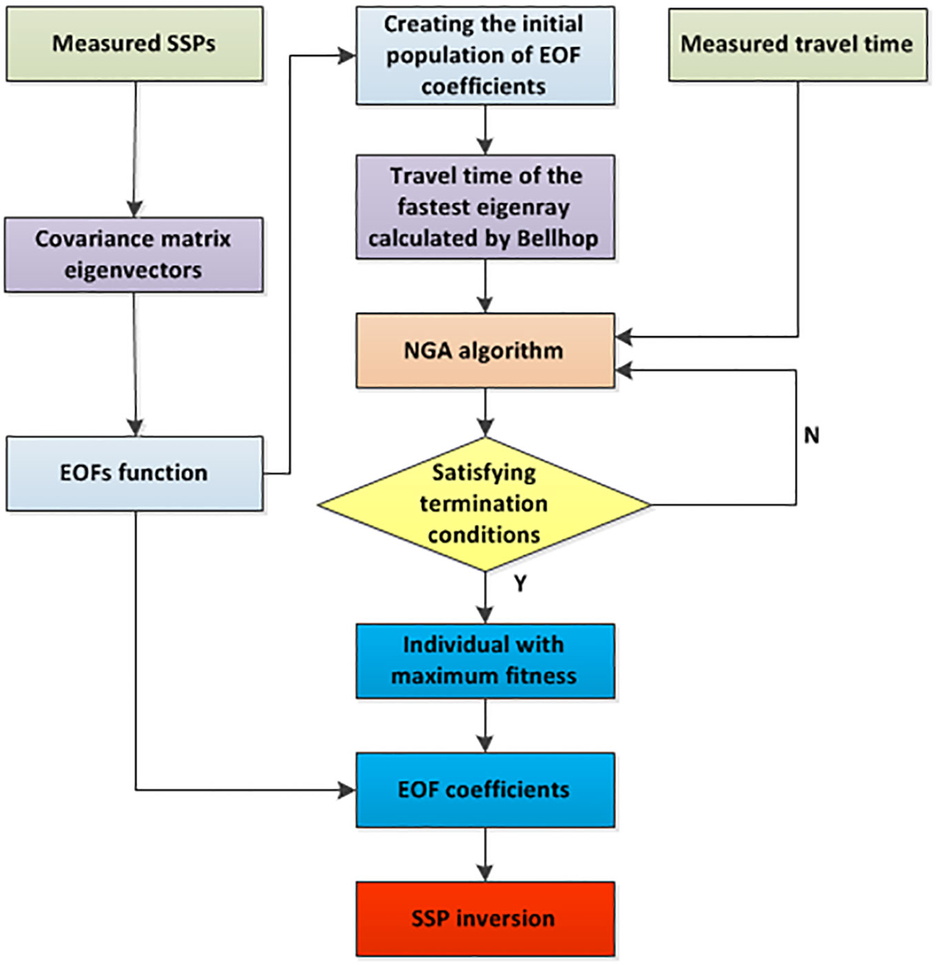
Figure 1 Schematic diagram of Niche Genetic Algorithm.
where is the calculated value of the travel time of the fastest characteristic sound rays received by each hydrophone using Bellhop model; is the travel time measured during the experiment (k=1, 2, 3…, K), and K is the number of the hydrophones;
4) Sort the individuals in descending order according to their fitness , and mark the first N (N<M) individuals;
5) Apply selection, crossover, and mutation operations to the population of M individuals;
6) Execute a niche elimination operation by combine the M individuals obtained in Step 5 with the first N individuals from Step 4, resulting in a new population of M+N individuals. Calculate Hamming distance between each pair of individuals and in the new population according to the following equation:
where represents the k-th variable of the i-th individual. When Hamming distance is less than L, the individuals with lower fitness in and are subject to a penalty function to reduce their fitness values;
7) From the population of M + N individuals, select the first M individuals with higher fitness values to generate the new population. If the termination condition has been met, the result is considered as the final output of NGA. Otherwise, repeat Step 3-6.
The observation data from targeted observation is incorporated into 3D-Var system to improve the ICs. Numerical simulations of ocean circulation patterns are assimilated with data the ocean environment observed by a wide range of instruments, guided by the statistical Bayesian conditional probability theory, to produce new numerical results. Such assimilated numerical results for the ocean environment contain both the extrapolation of the thermodynamic equations of ocean dynamics and the observed scenarios of the real state of the ocean environment. The numerical ocean model compensates for the shortcomings of the observations, which are always scattered and relatively sparse, and the observations control the uncertainties brought about by the non-linearities in the ocean dynamics and thermodynamic equations.
3D-Var aims to achieve an optimal state solution by minimizing the cost function. The equation of the cost function is as follows:
where x is the analysis variable; is the background field; is the observation value; is the background error covariance; is the observation error covariance; is the observation operator; is the inverse matrix of the corresponding matrix; is the transpose of the corresponding matrix; and L is the filter operator. In this study, “Analysis variable” refers to the vertical temperature profile result from assimilation. “Background field” refers to the prediction of temperature profile obtained from the ROMS model. “Observation value” refers to the XBT measured temperature profile. The observation update residuals are collected and spatially filtered by the filtering operator L, and the results are fed back to the grid point where the state x is located. L can be calculated as follows:
where a is the characteristic distance of the observation response; b is the distance between the observation point and the model grid point; and K is the total number of observations. Parameter a determines the scale of the multiscale method, and also the reduction ratio of each level of the scale grid to the original pattern grid when the grid varies.
The process of assimilation can be summarized as follows,
1) Observation: quality control of acquired data and production of observation data sets;
2) Assimilation: the observation dataset and model results are fed into the assimilation system module, which performs scale-by-scale 3D variational assimilation after grid transformation.
3) Forecasting: the assimilation results are substituted into the ocean model as initial values to obtain new numerical forecasts.
In this study, the process of ‘Observation - Assimilation - Forecasting’ is repeated with the number of observation cycles.
An experiment was conducted in August 2019 on the northwest continental slope of the Yellow Sea with the objective of improving short-term (7-day) thermal structure predictions during the summer season. The experiment consisted of two main components: OAT and targeted observation sections.
The targeted observation experiment was conducted from 18th to 25th August with the aim of improving short-term (7-day) thermal structure predictions. The experiment focused on a selected target region, denoted by a red box in Figure 2, which is located near the margin of Yellow Sea Cold Water Mass (YSCWM). In this region, Vertical Thermal Structure (VTS) is influenced by various dynamic processes, as well as complex topography. Consequently, the prediction of VTS in this region is associated with significant uncertainties (Hu et al, 2021). To determine the sensitive areas within the target region, an adjoint-free CNOP algorithm was employed. The identified sensitive areas were found to be oriented northeast to southwest, extending from the northeast towards the target region. These sensitive areas are likely influenced by the southwestward background currents.
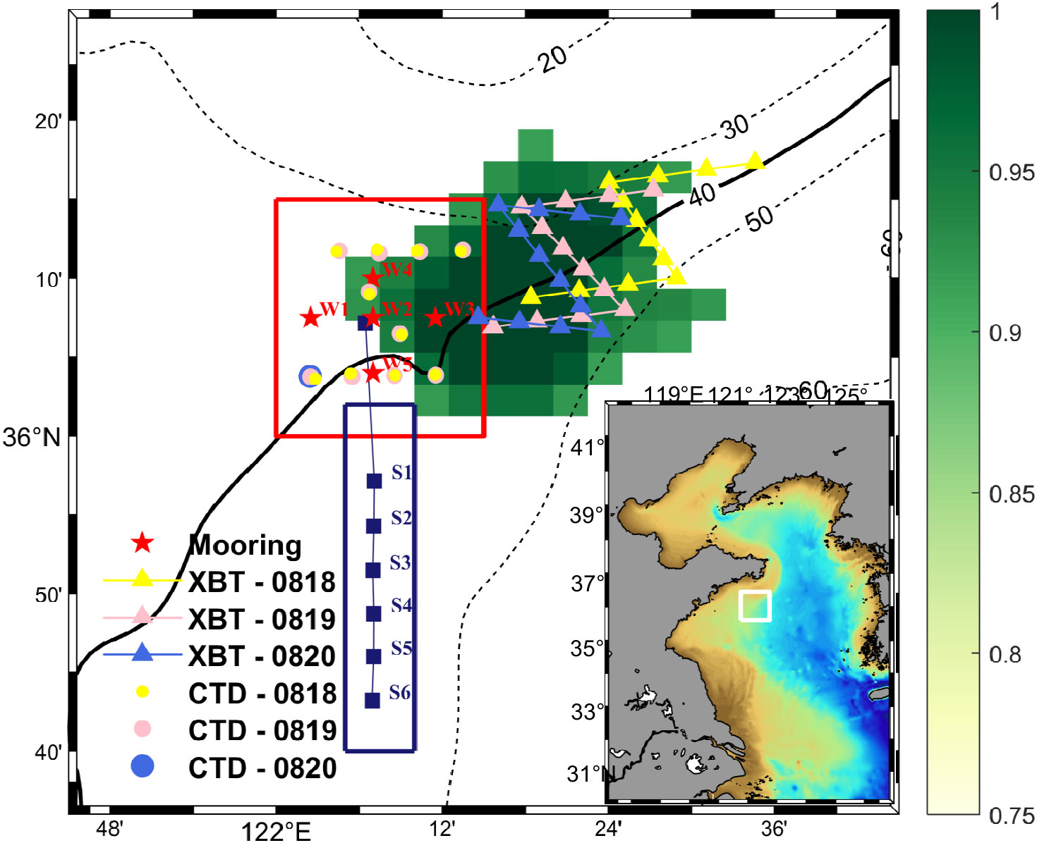
Figure 2 Schematic diagram of the experiment. The red open rectangle indicates the location of the target region of targeted observation experiment. The green area is the sensitive area in which the data were obtained on 20 August during CNOP, and which is extended from northeast to southwest towards the target region. The red closed stars indicate five temperature profile buoy stations, carried out during Aug 18-25. The yellow, grey and blue closed triangles locate thirty-six XBT locations, obtained on Aug 18, 19 and 20, respectively, and the yellow, grey and blue closed circles locate twenty-one shipboard CTD stations, obtained at the same date allocation. The violet closed squares, accompanied by a vertical array of S1, S2, S3, S4, S5 and S6, indicates 6 fixed-depth explosive acoustic source locations for OAT experiment on Aug 20. The lower right figure shows the position of the ocean model domain, in which the white open rectangle indicates the position of the experiment.
In the target region, a total of 5 buoys were deployed to gather data for the experiment. These buoys were composed of temperature loggers and pressure–temperature–conductivity loggers, enabling the collection of temperature profile at a vertical interval of 2m. The sampling interval of loggers is 10 minutes. The collected data from the buoys in the target region were utilized for validation purposes. Furthermore, shipboard temperature, conductivity, and depth measurements were conducted, resulting in 21 temperature profiles measured within the targeted region. In the sensitive region identified through CNOP (green area in Figure 2), eXpendable Bathy Thermographs (XBT) were employed to collect temperature profiles 4 times a day (4:30-7:30, 10:30- 13:30, 16:30-19:30, 22:30-01:30) along predesigned routes (i.e., triangles in Figure 2). The data acquired from XBT in the time-varying sensitive area were then substituted into cycle data assimilation process to refine the prediction of the target region at the 7-th day following XBT deployment (verification time). The refined prediction obtained from this assimilation, as well as the basic prediction, were both compared against the data measured by the buoys in the target region. These comparisons served to verify the effectiveness of the targeted observation approach. The experimental results demonstrated that observations within the identified sensitive area, which aimed at reducing initial errors, led to a more significant improvement in VTS prediction of the target region at the verification time compared to similar actions conducted solely within the target region itself (Hu et al, 2021; Liu et al, 2021). This study focuses on the application of acoustic tomography in targeted observation, and as such, the conclusions of the targeted observation experiment will not be repeated.
OAT experiment was designed to validate the feasibility of acoustic tomography for the inversion of the marine environment. The experiment was carried out on August 25 in the southern region of the targeted observation experiment, as denoted by the blue box in Figure 2. NGA algorithm was employed to invert SSP using acoustic travel time data. Subsequently, based on OACM, the corresponding temperature profile was calculated through the inversion of SSP obtained from NGA algorithm.
A launching ship was employed during the experiment to deploy fixed-depth explosive as the acoustic source. The launching ship moved away from the receiving ship and followed a predetermined trajectory from point S1 (approximately 10 nautical miles away from the receiving ship) to point S6 (approximately 22.5 nautical miles). At intervals of 2.5 nautical miles along this trajectory, the launching ship came to a halt and dropped 3 kinds of bombs at controlled depths: 7, 25, and 35m. The depths of explosions and distances between launching and receiving ships are shown in Table 1. To capture the acoustic signals generated by the explosions, a standard hydrophone was fixed at a depth of 10m on the stern of the launching ship. This hydrophone was utilized to record the explosion time and the corresponding source level.
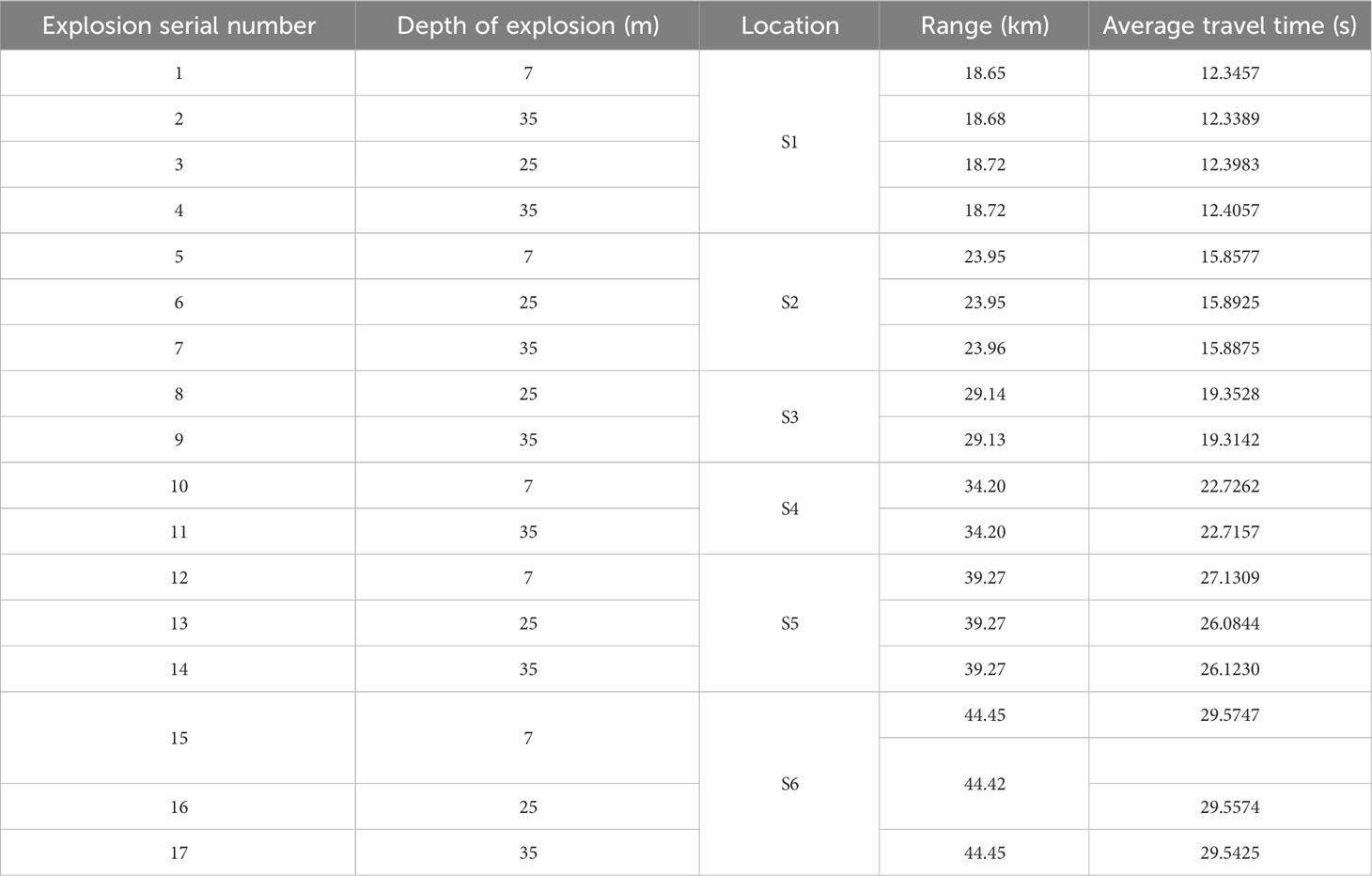
Table 1 Depths of explosions and distances between launching and receiving ships.
On the receiving ship, a vertical array comprising 15-element hydrophones was deployed on the port aft deck. The hydrophone array spanned depths ranging from 5 to 33m, with a uniform interval of 2m. The receiving ship remained anchored at a fixed position throughout the experiment, enabling the recording of the acoustic signals. The schematic diagram of OAT experiment is shown in Figure 3. Examples of signals received by hydrophones are shown in Figure 4.
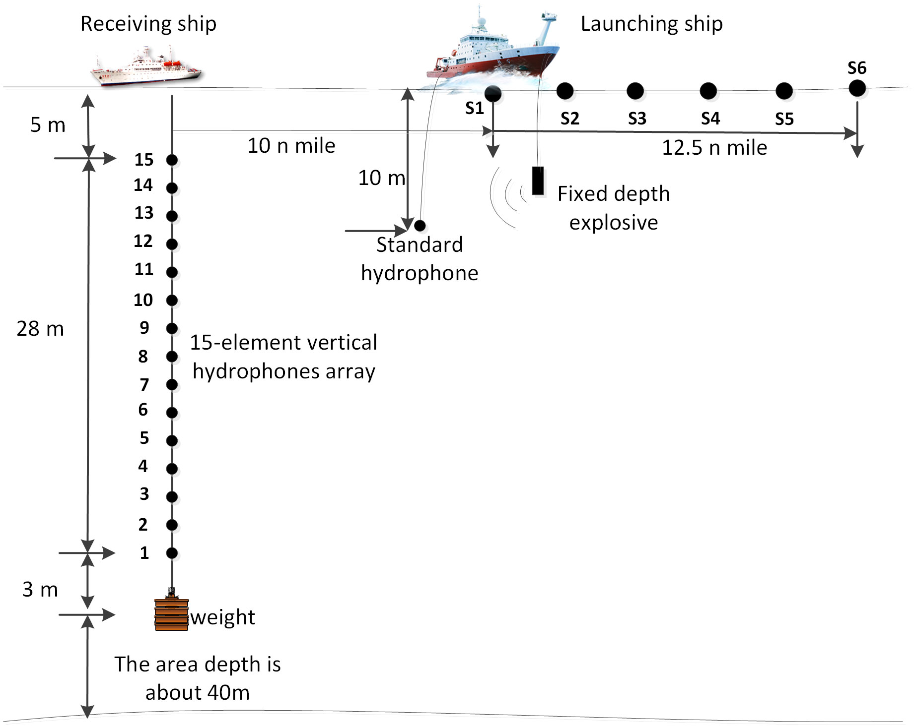
Figure 3 Schematic diagram of OAT experiment. Launching ships dropped fixed-depth explosive at specific ranges, while the explosion time were recorded using a hydrophone fixed at the stern. Receiving ship recorded acoustic signals with a 15-element vertical hydrophones array at a fixed location.
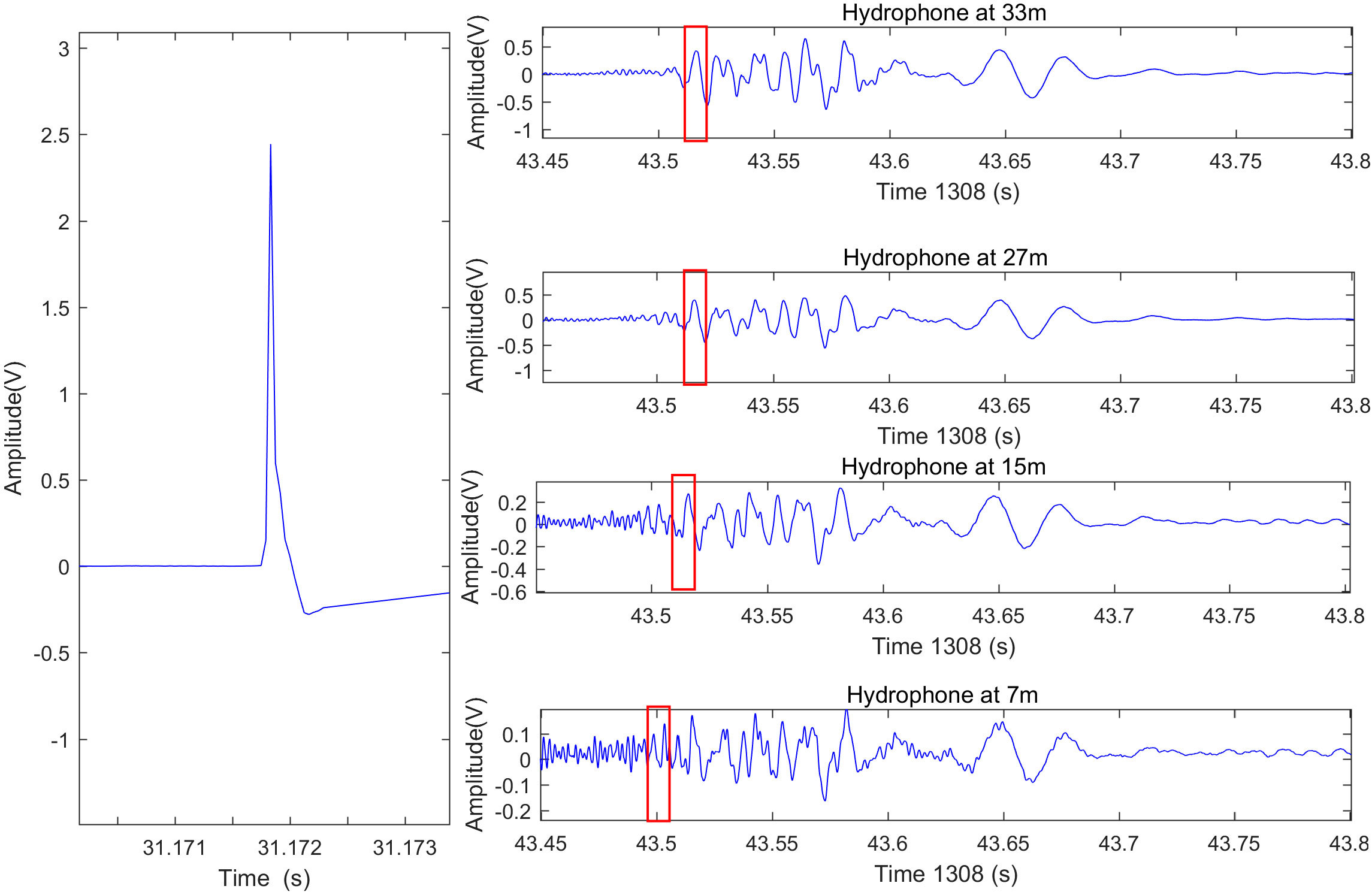
Figure 4 Examples of signals received by hydrophones on the launching and receiving ships. The figure on the left is the signal example received by the hydrophone on the launching ship. The figures on the right are the signal examples received by the receiving ship at point S1, 33m, 27m, 15m, and 7m depth hydrophones from top to bottom. The horizontal axis is the time axis, 1308 means 13:08 p.m., and the values under the horizontal axis represent the corresponding seconds.
Both the launching and receiving vessels were equipped with a multi-channel hydroacoustic signal synchronization acquisition system. This system facilitated the acquisition of the explosion sound source signals from the launching ship and the hydroacoustic signals recorded by the hydrophone array on the receiving ship. Importantly, the embedded a GPS module, enabling the acquisition of precise GPS clock information and position data for real-time synchronization of the explosion sound source signals. This synchronization ensured accurate temporal alignment between the recorded acoustic signals and facilitated reliable analysis of the acoustic data obtained during the experiment.
The steps of inverting the ocean environment in section 2.2 were executed as follows:
1) A total of 29 SSPs were measured by the launching and receiving ships during the OAT experiment. The covariance matrix eigenvectors and eigenvalues of these SSPs were computed. As the largest three eigenvalues accounted for more than 95% of the sum of all the eigenvalues, so the 3-order EOFs was used. The eigenfunctions corresponding to top 3 eigenvalues are the EOF functions. The EOF coefficients of every SSP were calculated;
2) The EOF coefficients obtained above were augmented with a normal perturbation to generate an initial population with a population size of 500. The population size of 500 was found in the simulations to cover the variable space of the EOF coefficients well and achieve as large a diversity of populations as possible;
3) The positioning and timing information is obtained through synchronous GPS data collected by the standard hydrophone on the launching ship and the hydrophone array on the receiving ship. The travel time of the acoustic signal is calculated using the first wave peak of the signal received by the receiving ship and the signal pulse received by the launching ship. A matched filter algorithm was used to determine the travel times of different eigenrays and the eigenray with the min travel time is consider as the fastest eigenray. The time obtained above is considered as the travel time of the fastest eigenray (Table 1). It’s worth mentioning that there is a distance (30m) between the bomb launching point and the hydrophone on the launching ship. So, an extra delay is added on travel time. Considering that the depth of 0-15m is a homogeneous layer and the speed of sound is 1535m/s, it is necessary to add another 0.0195s to the travel time. In this way, the in equation (1) is calculated. Subsequently, the BELLHOP acoustic model is employed to calculate the intrinsic acoustic propagation delay from the sound source to each hydrophone i.e., in equation (1). Thus, the fitness of the individuals of each population was calculated according to equation (1);
4) The 500 individuals were sorted by and the top 100 individuals were labelled, i.e., the crowding factor was set to 1/5 (De Jong, 1975; Zhang, 2013; Cui et al, 2021);
5) Selection, crossover and mutation operations of genetic algorithm were performed on all 500 individuals to produce the next generation. The maximum number of genetic generations was set to be 40, the mating probability to be 0.5, the mutation probability to be 0.2. The parameters are the result of a comprehensive consideration after simulation, which takes into account both the need to traverse the entire search space and also the computational efficiency;
6) The Hemming distances between the 500 individuals generated in the step 5 and the 100 individuals labeled in the step 4 were calculated according to equation (2). The less adapted of the two individuals within specific distance was penalized. Thus, 500 individuals (out of 500 + 100 individuals above) with higher fitness are the next generation.
The above steps were repeated until the fitness function of the optimal individual satisfied the termination condition, then the corresponding SSP of the optimal individual was output as the inversion result.
The SSP obtained from the experiments of 35m bombs at 6 release points (S1-S6) and measured data are selected as samples and shown in Figure 5. The measured data are XBT measurement from launching and receiving vessels during the experiment. Due to the limited availability of salinity data (only 2 CTD measurements per buoy), the salinity profile is assimilated with measured data based on ROMS dataset, shown in Figure 6A. The average SSP of OAT is shown in Figure 6B. Consequently, the temperature profile is extracted using OACM and illustrated in Figure 6C. Figure 6 reveals that the biases primarily originate in the thermocline depth, while the biases in the sea surface mixed layer and deeper layers are relatively smaller. Root Mean Square Error (RMSE) for SSP and temperature profile is calculated to be 1.07m/s and 0.40°C, respectively. Specifically, RMSE in thermocline depth (15-40m) is 1.21m/s and 0.47°C. These results are considered accurate, taking into account the limited number of blast sources and the duration of the experiment. The findings suggest that NGA algorithm-based OAT can reliably invert the marine environment in Yellow Sea.
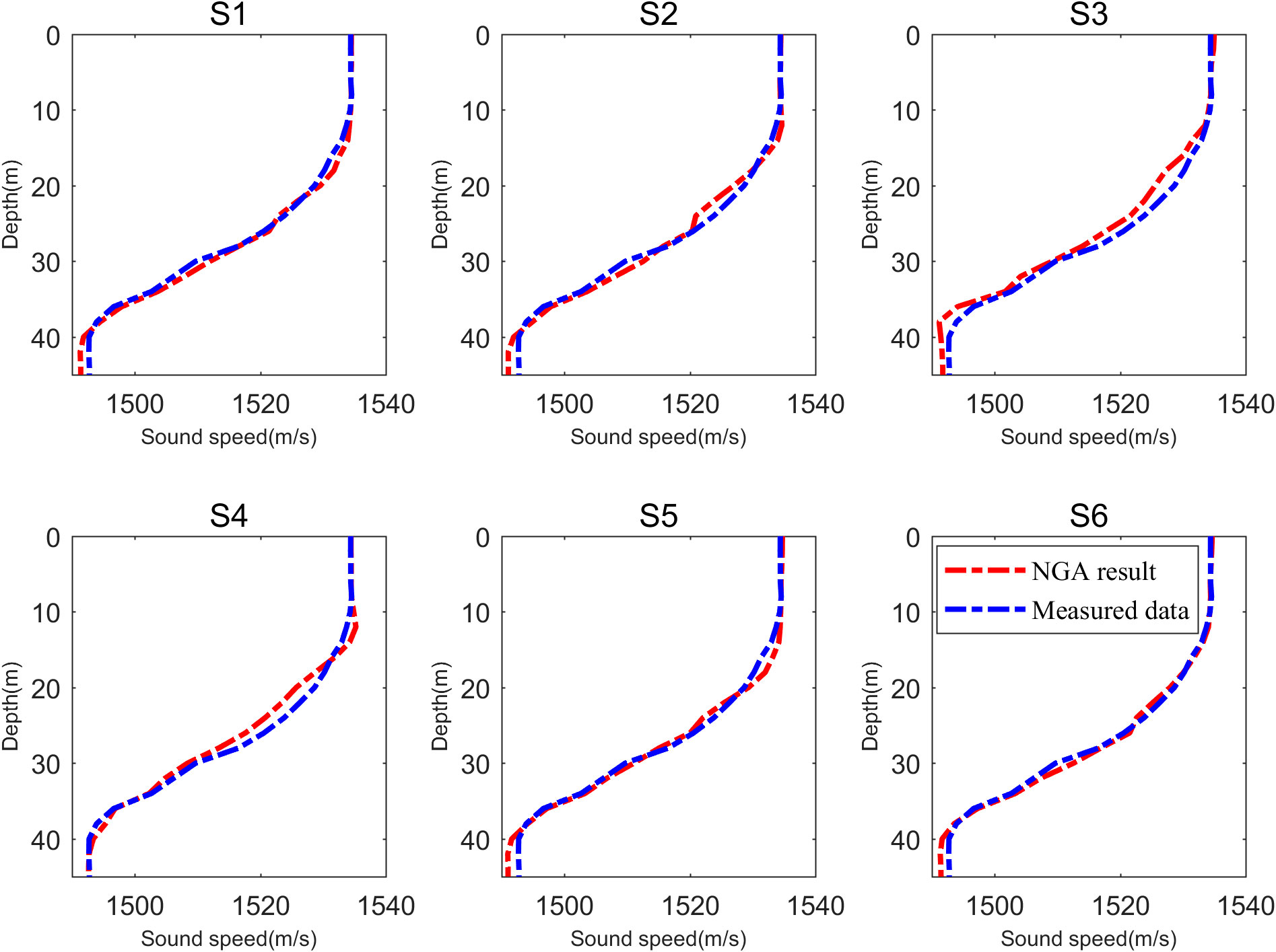
Figure 5 Comparisons of NGA results and measured data obtained from the experiments of 35m bombs at 6 release points (S1-S6).
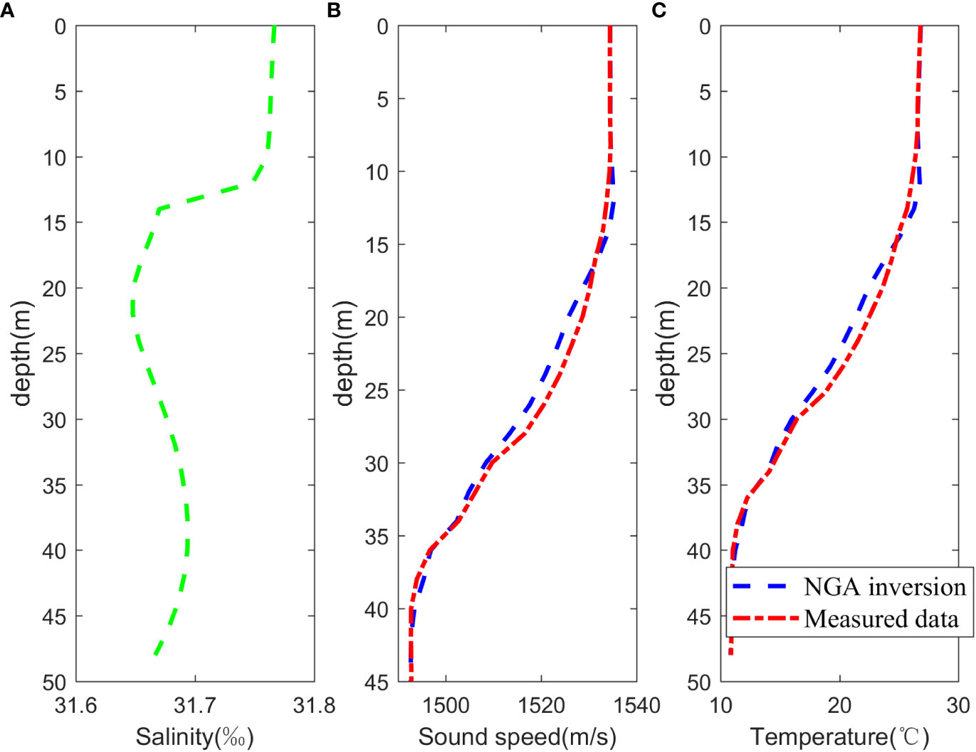
Figure 6 Results of OAT inversion. (A) Salinity profile after assimilation with measured data based on ROMS dataset, (B) Comparison of average SSP obtained from OAT and measured data, (C) Comparison of average temperature profiles obtained from OAT and measured data.
As OAT experiment was not conducted within the sensitive area of targeted observation, a simulation experiment was employed to verify the impact of OAT on ocean environment prediction.
Considering the variation characteristics of temperature in the OAT experiment area and the sensitive area are quite different, it’s irrational to assimilate OAT inversion result as targeted observation data directly. In this study, the temperature bias obtained from the acoustic tomography inversion and the temperature measurement data from XBT in the sensitive area were combined to simulate the acoustic tomography inversion data within the sensitive area. The vertical bias structure is related only to the OAT inversion method, but not the region. Thus, the simulated observations of “truth + bias” avoid the influence of the bias in different regions on the results. These simulated OAT observation data were then brought into the assimilation system to obtain updated ICs, leading to improved predictions through the use of 3D-Var and ROMS methods. The prediction results at the verification time were compared between the basic prediction, the measured data from buoys in the target region (noted by red stars in Figure 2), the assimilation of XBT measured data, and the assimilation of the simulated OAT assimilation. The comparison results are shown in Figure 7.
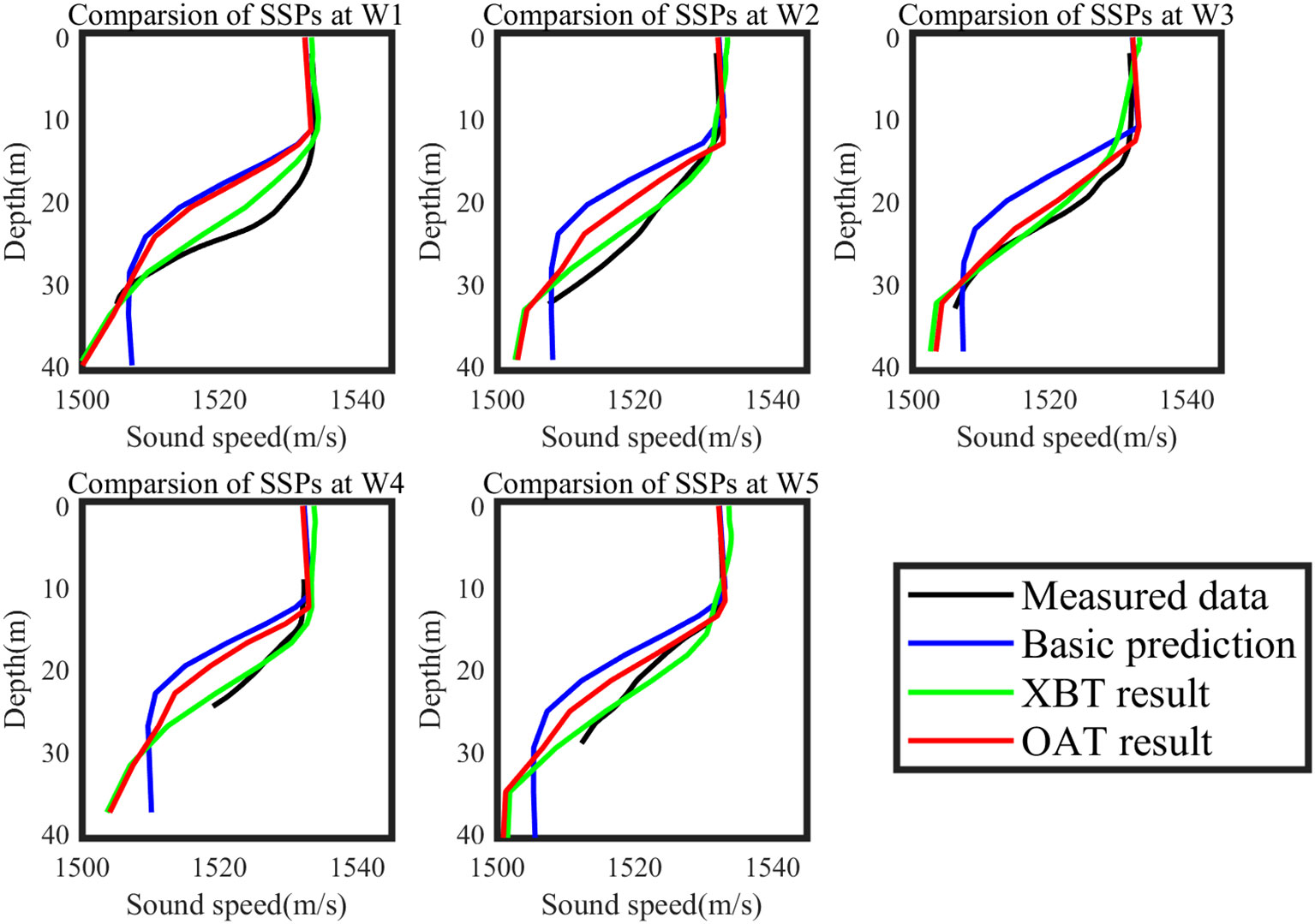
Figure 7 Comparisons of sound speed profile at different buoy station at verification time (day 7), including measured data (black line), basic prediction (blue line), assimilation results from XBT measured data (green line) and assimilation results from OAT inversion simulation data (red line).
The results demonstrate that both the simulated OAT observation and Exp observation(XBT result) significantly improve the accuracy of temperature profile forecasts compared to the basic prediction at the verification time. These results are closer to the measured data, particularly in surface and thermocline layers. It should be noted that the comparison does not include the deeper layers since the buoy depths do not reach the seafloor. RMSEs of the basic prediction, Exp, and OAT simulation data compared to the measured data at 5 buoys are calculated and presented in Table 2. Overall, Exp yields more accurate results than OAT simulation data, primarily due to the introduced bias of OAT inversion. On average, RMSE of XBT prediction is reduced by 68.1%, while RMSE of OAT prediction is decreased by 49.9% comparing with basic prediction. On the other hand, setting VTS at W3 buoy as an example, the RMSEs of these predictions along with a Ctrl Run, which is the result of assimilation based on observation in the target region, are shown in Figure 8. From Figure 8, the bias of XBT and OAT results change on a similar trajectory. At the verification time, the RMSE in the target region was greatly reduced by experiment with deploying XBT observation and simulated OAT observation in the identified sensitive area (XBT result and OAT result) than that of experiment with observations being deployed in the verification area itself (Ctrl Run). These findings demonstrate that OAT can serve as a reliable observation method for targeted observation.
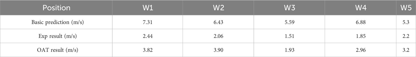
Table 2 RMSEs of basic prediction, experimental data, and OAT data compared with measured data in the target region at 7-th day.
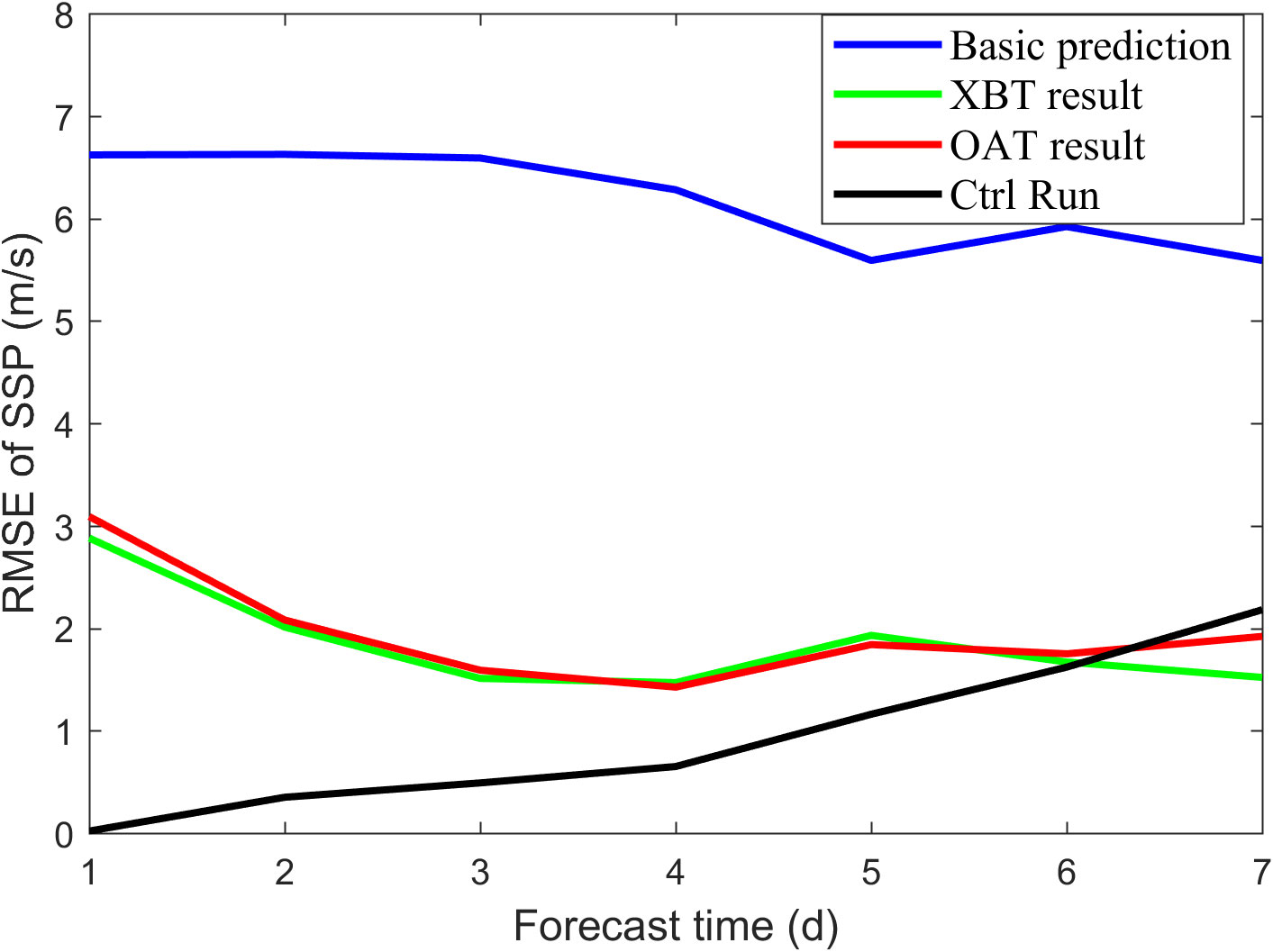
Figure 8 Temporal evolution of vertical integration RMSEs of SSP at W3 station, including basic prediction (blue line), assimilation results from XBT measured data in sensitive area (green line), OAT inversion simulation data in sensitive area (red line) and measured data in the target region (Ctrl Run-black line).
The simulation experiment described above provides validation regarding the influence of OAT data from XBT locations. However, the unique characteristics of acoustic tomography, including its large-area coverage and long-term observation capabilities under low-cost conditions, necessitate further verification of OAT’s influence on prediction using OSSE. For the OSSE, two sets of predictions with different ICs and same driving conditions are selected: “True Run” and “Ctrl Run”. “True Run” and “Ctrl Run” are predictions from same boundary and driving conditions, but different initial conditions. “True Run” is regarded as the real ocean measured data. “Ctrl Run” is regarded as the basic prediction without additional observation. Targeted observation data from the sensitive area, extracted from “True Run”, is combined with OAT inversion bias to simulate OAT targeted observation data. This OAT targeted observation data is then assimilated with data from “Ctrl Run” using 3D-Var system, resulting in the generation of “Exp Run”. By comparing the predictions of “Ctrl Run” and “Exp Run” with “True Run” at the verification time, the impact of OAT as a targeted observation method on prediction can be analyzed (Figure 9). To further investigate the effect of OAT observations on prediction quality under different conditions, various experiment setups were employed. EXP1 replicates the same OAT observation condition as XBT measurement. Observations were carried out at the locations of the triangular markers of the three Z-lines in the sensitive area of Figure 2 from day 1 to day 3. EXP2 simulates observation on all ocean model nodes in the sensitive area, meaning the observation area is 4 times the area of EXP1, while the observation keeps the same(day 1-3). EXP3 takes observation in the same area as EXP1 while the observations time is extended, which indicates that observations are located on the triangular locations from day 1 to day 5. EXP4 is the combination of EXP2 and EXP3, i.e., observations are carried out on all ocean model nodes in the sensitive area from day 1 to day 5. The results of these experiments are depicted in Figure 10 and Table 3.
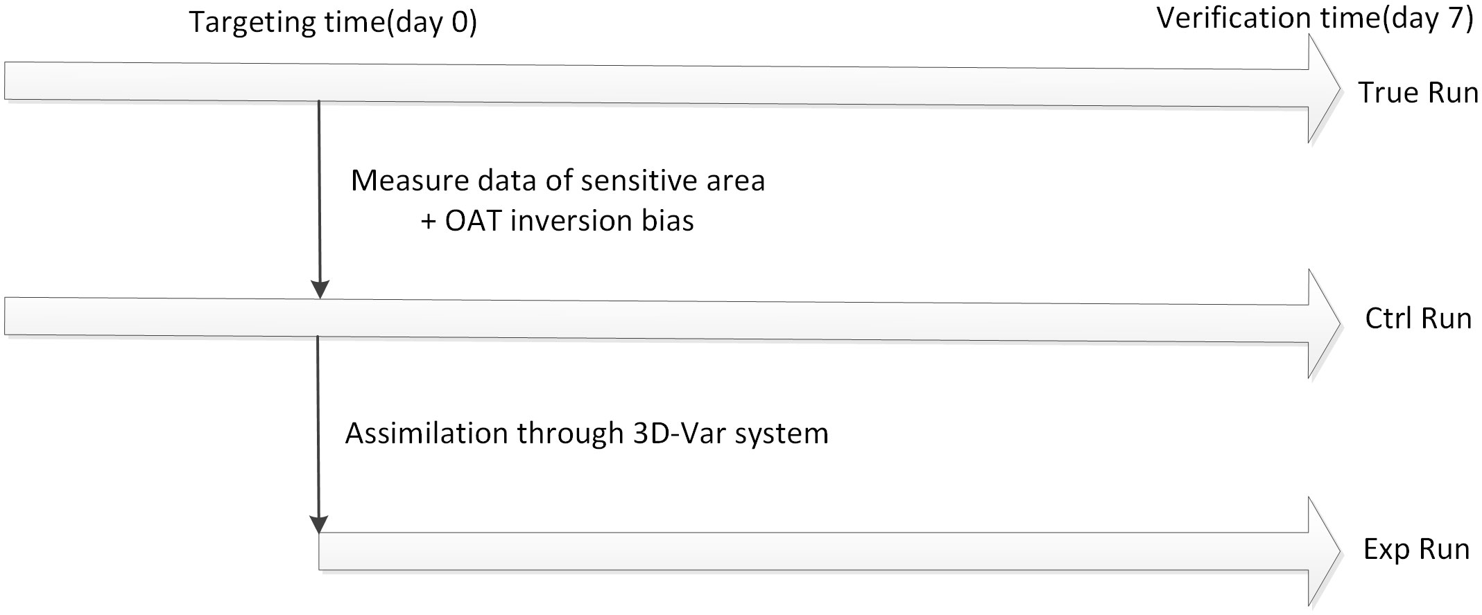
Figure 9 Schematic diagram of Observing System Simulation Experiments (OSSE). Targeted observation data from the sensitive area at the targeting time is extracted from “True Run”. This data is then combined with OAT inversion bias and assimilated with data from “Ctrl Run” to generate “Exp Run”.
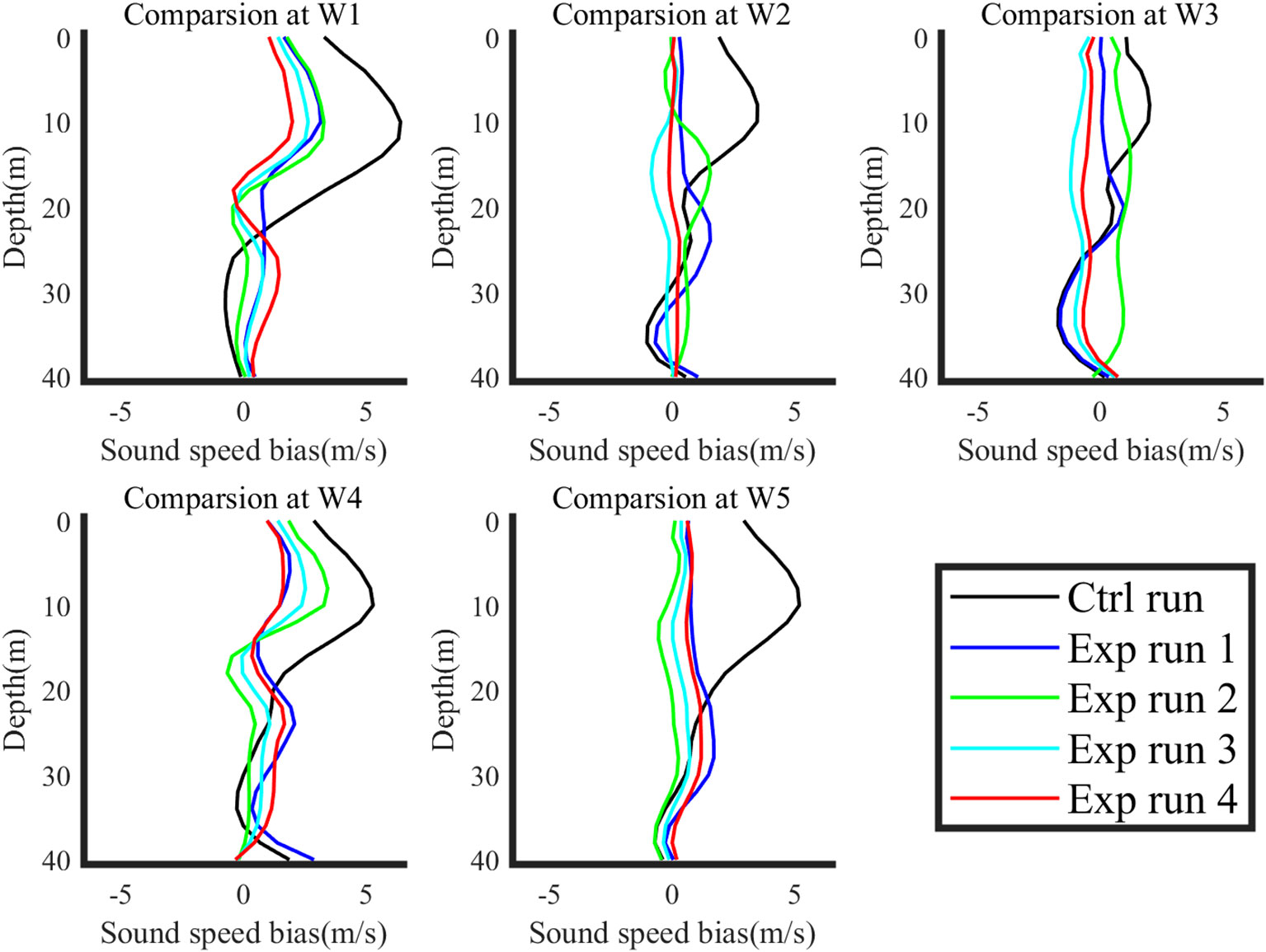
Figure 10 Results of OSSE. Vertical sound speed bias structures of different experiment conditions are configured, including Ctrl Run (black line), EXP1 for basic OAT observation (blue line), EXP2 for larger observation area (green line), EXP3 for extended observation time (black line), and EXP4 for both a larger observation (cyan line) area and an extended observation time (red line).
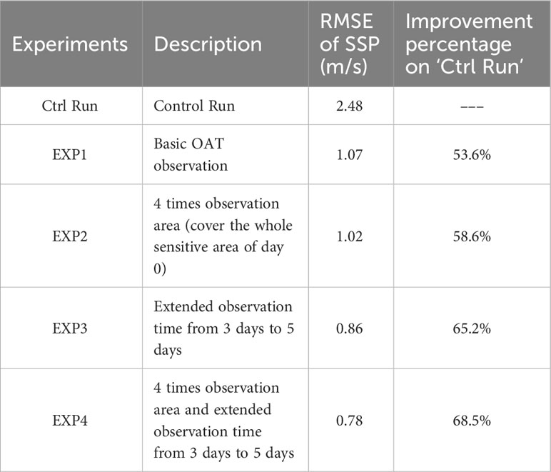
Table 3 Setup and results of OSSE.
The results of EXP1 reinforce the finding that OAT can improve prediction quality, thereby validating its utility as a targeted observation method. EXP2 and EXP3 demonstrate that increasing the observation area and extending the observation time further improve the prediction quality. However, it is observed that the enhancement in prediction quality is more pronounced with an extended observation time. This phenomenon can be attributed to the fact that both the horizontal resolution of the ocean model employed and the assimilation radius of the 3D-Var system exceed the observation spacing. Consequently, expanding the observation area may not yield enough additional valuable environmental information. Conversely, extending the observation time not only provides more observations but also reduces the time interval between the final observations and the verification time. EXP4 results reveal that the combination of increasing the observation area and extending the observation time improves the prediction quality for maximum. However, improvement achieved through this approach is not notably different from that achieved solely by extending the observation time. Furthermore, extending the observation time is more cost-effective and logistically feasible compared to deploying additional observation nodes during sea trials. Consequently, prolonged observations duration emerges as an efficient and economical approach to observation, thereby offering reference for the implementation of acoustic tomography targeted observation projects.
OAT is a cost-effective, long-term, and wide-area ocean monitoring method that obtains acoustic signals to invert marine environment characteristics. In this study, the validity of OAT for the marine environment inversion was verified using data collected during the 2019 Yellow Sea experiment. The OAT inversion biases were incorporated into measurements obtained from the sensitive area, identified by CNOP method, to simulate OAT observations from the sensitive area. These simulated OAT observations were substituted into a 3D-Var assimilation system to improve the quality of ICs and subsequently enhance the short term (7-day) prediction of the target region. These findings confirm the effectiveness of OAT as a targeted observation method. Considering the large-scale and long-duration nature of OAT, OSSE method was employed to further test the impact of OAT on prediction quality. Specifically, the effects of adding observation nodes and extending the observation duration were examined. The results show that both approaches and their combination have positive effects in reducing prediction uncertainty. However, it was found that extending the observation duration is a more efficient strategy.
This study aims to verify the feasibility of acoustic tomography as a targeted observation method in a simulated environment using actual measurement data. It is important to note that the findings of this study are yet to be validated in sea trials. Additionally, most existing acoustic tomography observation methods utilize fixed or submerged buoys, while the sensitive area for targeted observation changes with time. Therefore, it is crucial to investigate optimal selection strategies for observation nodes that can yield the highest improvement in prediction quality. Additionally, it is necessary to examine the effect of parameter variations in the ocean model and assimilation model on acoustic tomography and its corresponding targeted observations. Understanding the interrelationships and contribution of these parameters to the prediction quality requires further investigation.
The raw data supporting the conclusions of this article will be made available by the authors, without undue reservation.
CB: Formal Analysis, Methodology, Writing – original draft, Writing – review & editing. LJ: Data curation, Formal Analysis, Writing – review & editing. GW: Funding acquisition, Investigation, Resources, Writing – review & editing. DL: Funding acquisition, Resources, Writing – review & editing.
The author(s) declare financial support was received for the research, authorship, and/or publication of this article. This research received support by National Basic Research Program of China (Grant Number 2019-JCJQ-ZD-149-00) and Taishan Scholars Program.
We are grateful to Liu Kun for his help in ocean model building, Hu Huiqin for her assistance in assimilation system, the captains Bing Liu, Xiufeng Chen and all the crews of the R/V KeXue No. 3 and R/V ChuangXin No. 2 for their cooperation in collecting the observation data.
The authors declare that the research was conducted in the absence of any commercial or financial relationships that could be construed as a potential conflict of interest.
All claims expressed in this article are solely those of the authors and do not necessarily represent those of their affiliated organizations, or those of the publisher, the editors and the reviewers. Any product that may be evaluated in this article, or claim that may be made by its manufacturer, is not guaranteed or endorsed by the publisher.
Baker N. L., Daley R. (2000). Observation and background adjoint sensitivity in the adaptive observation-targeting problem. Q.J.R. Meteorol. Soc 126 (565), 1431–1454. doi: 10.1002/qj.49712656511
Bishop C. H., Etherton B. J., Majumdar S. J. (2001). Adaptive sampling with the ensemble transform kalman filter. Part I: theoretical aspects. Monthly Weather Review. 129 (3), 420–436. doi: 10.1175/1520-0493(2001)129<0420:ASWTET>2.0.CO;2
Buizza R., Montani A. (1999). Targeting observations using singular vectors. J. Atmospheric Sci. 56 (17), 2965–2985. doi: 10.1175/1520-0469(1999)056<2965:TOUSV>2.0.CO;2
Carrière O., Hermand J. P. (2008). A sequential Bayesian approach to vertical slice tomography of a shallow water environment. J. Acoustical Soc. America. 123 (5_Supplement), 3339–3339. doi: 10.1121/1.2933874
Chan P. W., Han W., Mak B., Qin X., Liu Y., Yin R., et al. (2022). ). Ground-space-sky observing system experiment during tropical cyclone mulan in August 2022. Adv.Atmos. Sci. 40 (2), 194–200. doi: 10.1007/s00376-022-2267-z
Cui B., Xu G., Da L., Guo W. (2021). Shallow sea sound speed profile inversion based on niche genetic algorithm. J. Appl. Acoustics 40 (2), 1–8. doi: 10.11684/j.issn.1000-310X.2021.02
Da L., Guo W., Zhao J., Fan P. (2015). Capture uncertainty of underwater environment by ocean-acoustic coupled model. Acta Acustica. 40 (3), 477–486. doi: 10.15949/j.cnki.0371-0025.201
Dahl P. H., Zhang R., Miller J. H., Bartek L. R., Peng Z., Ramp S. R., et al. (2004). Overview of results from the asian seas international acoustics experiment in the east China sea. IEEE J. Oceanic Engineering. 29 (4), 920–928. doi: 10.1109/JOE.2005.843159
DeFerrari H. A., Nguyen H. B. (1986). ). Acoustic reciprocal transmission experiments, Florida Straits. J. Acoust Soc. Am. 79 (2), 299–315. doi: 10.1121/1.393569
De Jong K. A. (1975). An analysis of the bechavior of a class of genetic adaptive systems (MI, United States: University of Michigan). Ph. D Dissertation.
Duan W., Hu J. (2015). The initial errors that induce a significant “spring predictability barrier” for El Nino ˜ events and their implications for target observation: results from an earth system model. Clim. Dynam. 46 (11–12), 3599–3615. doi: 10.1007/s00382-015-2789-5
Duan W. S., Mu M. (2018). Predictability of el nino-southern ˜ Oscillation events. OXFORD research encyclopedia, CLIMATE SCIENCE. (United States: Oxford University). Available at: https://climatescience.oxfordre.com. doi: 10.1093/acrefore/9780190228620.013.80
Duda T. F., Lynch J. F., Newhall A. E., Wu L., Chiu C. S. (2004). Fluctuation of 400-hz sound intensity in the 2001 ASIAEX south China sea experiment. IEEE J. Oceanic Engineering. 29 (4), 1264–1279. doi: 10.1109/joe.2004.836997
Dushaw B. D. (1999). “The Acoustic Thermometry of Ocean Climate (ATOC) Project: Towards depth-averaged temperature maps of the North Pacific Ocean,” in Proceeding of the International Symposium on Acoustic Tomography and Thermometry, Tokyo, Japan. doi: 10.1121/1.413035
Dushaw B., Forbes A., Gaillard F., Gavrilov A., Gould J., Howe B., et al. (2001). “Observing the ocean in the 2000’s: A strategy for the role of acoustic tomography in ocean climate observation,” in Observing the oceans in the 21st century (University of Washington,United States: GODAE Project Office and Bureau of Meteorology).
Dushaw B. D., Worester P. F. (2001). “Acoustic remote sensing of the North Pacofic on gyre and regional scales,” in Pacific CLIVAR international Pacific Implementation Workshop, International Pacific Research Center at the University of Hawaii, Honolulu, Hawaii.
Feng R., Duan W., Mu M. (2016). Estimating observing locations for advancing beyond the winter predictability barrier of Indian Ocean dipole event predictions. Climate Dynamics. 48 (3-4), 1173–1185. doi: 10.1007/s00382-016-3134-3
Feng Y., Min J., Zhuang X., Wang S. (2019). Ensemble sensitivity analysis-based ensemble transform with 3D rescaling initialization method for storm-scale ensemble forecast. Atmosphere. 10, 24. doi: 10.3390/atmos10010024
Fried S., Walker S., Hodgkiss W., Kuperman W. (2013). Measuring the effect of ambient noise directionality and split-beam processing on the convergence of the cross-correlation function. J. Acoustical Soc. America 134 (3), 1824–1832. doi: 10.1121/1.4816490
Gasparini O., Camporeale C., Crise A. (1997). Introducing passive matched field acoustic tomography. Nuovo Cimento- Societa Italiana di Fisica Sezione C. 20 (4), 497–520.
Hamill T. M., Snyder C. (2002). Using improved background-error covariances from an ensemble kalman filter for adaptive observations. Monthly Weather Review. 130 (6), 1552–1572. doi: 10.1175/1520-0493(2002)130
Howe B. M. (1987). Multiple receivers in single vertical slice ocean acoustic tomography experiments. J. Geophysical Research: Oceans. 92 (C9), 81–86. doi: 10.1029/JC092iC09p09479
Howe B. M., Mercer J. A., Spindel R. C., Worcester P. F., Hildebrand J. A., Hodgkiss W. S., et al. (1991). “Slice89: A single slice tomography experiment,” in Ocean variability & Acoustic propagation. Eds. Potter J., Warn-Varnas A. (Dordrecht: Springer). doi: 10.1007/978-94-011-3312-8_6
Hu H., Liu J., Da L., Guo W., Liu K., Cui B. (2021). Identification of the sensitive area for targeted observation to improve vertical thermal structure prediction in summer in the Yellow Sea. Acta Oceanologica Sinica. 40 (7), 77–87. doi: 10.1007/s13131-021-1738-x
Huang C.-F., Yang T. C., Liu J.-Y., Schindall J. (2013). Acoustic mapping of ocean currents using networked distributed sensors. J. Acoustical Soc America 134, 2090–2105doi: 10.1121/1.4817835
Jin G., Lynch J., Pawlowicz R., Wadhams P. (1993). Effects of sea ice cover on acoustic ray travel times, with applications to the Greenland Sea Tomography Experiment. J. Acoust Soc. Am. 94 (2), 1044–1057. doi: 10.1121/1.406951
Joly A., Browning K. A., Bessemoulin P., Cammas J., Caniaux G., Chalon J., et al. (1999). Overview of the field phase of the fronts and Atlantic Storm-Track EXperiment (FASTEX) project. Quarterly Journal of the Royal Meteorological Society. 125 (561), 3131–3163. doi: 10.1002/qj.49712556103
Kramer W., Dijkstra H. A., Pierini S., van Leeuwen P. J. (2012). Measuring the impact of observations on the predictability of the kuroshio extension in a shallow-water model. J. Phys. Oceanography. 42 (1), 3–17. doi: 10.1175/JPO-D-11-014.1
Langland R., Tóth Z., Gelaro R., Szunyogh I., Shapiro M., Majumdar S., et al. (1999). The north pacific experiment (NORPEX-98): targeted observations for improved north american weather forecasts. Bull. Amer Meteorol Soc 80, 1363–1384. doi: 10.1175/1520-0477(1999)080<1363:TNPENT>2.0.CO;2
Lebedev K. V., Yaremchuk M., Mitsudera H., Nakano I., Yuan G. (2003). Monitoring the kuroshio extension with dynamically constrained synthesis of the acoustic tomography, satellite altimeter and in situ data. J. Oceanography. 59 (6), 751–763. doi: 10.1023/B:JOCE.0000009568.06949.c5
Li F., Guo X., Hu T., Ma L. (2014). Acoustic travel-time perturbations due to shallow-water internal waves in the Yellow Sea. J. Comput. Acoustics. 22, 1–11. doi: 10.1142/S0218396X14400037
Li F., Yang X., Zhang Y., Luo W., Gan W. (2019). Passive ocean acoustic tomography in shallow water. J. Acoustical Soc. America. 145 (5), 2823–2830. doi: 10.1121/1.5099350
Liu K., Guo W., Da L., Liu J., Hu H., Cui B. (2021). Improving the thermal structure predictions in the Yellow Sea by conducting targeted observations in the CNOP-identified sensitive areas. Sci. Rep. 11 (1), 19518. doi: 10.1038/s41598-021-98994-7
Liu J. Y., Liu K., Guo W. H., Liang P., Da L. L. (2023). Optimal initial errors related to the prediction of the vertical thermal structure and their application to targeted observation: A 3-day hindcast case study in the northern South China Sea. Deep Sea Res. Part I: Oceanographic Res. Papers. 200, 104146. doi: 10.1016/j.dsr.2023.104146
Lynch J. F., Jin G., Pawlowicz R., Ray D., Plueddemann A. J., Chiu C. S., et al. (1996). Acoustic travel-time perturbations due to shallow-water internal waves and internal tides in the Barents Sea Polar Front: Theory and experiment. J. Acoust Soc. Am. 99 (2), 803–821. doi: 10.1121/1.414657
Malfoud S. W. (1995). Niche methods for genetic algorithms (Illinois: University of Illinois, Urbana-Champain).
Mu M. (2013). Methods, current status, and prospect of targeted observation. Sci. China Earth Sci. 56 (12), 1997–2005. doi: 10.1007/s11430-013-4727-x
Mu M., Duan W. S., Wang B. (2003). Conditional nonlinear optimal perturbation and its applications. Nonlin. Processes Geophys. 10 (6), 493–501. doi: 10.5194/npg-10-493-2003
Munk W., Worcester P. F., Wunsch C. (1995). Ocean acoustic tomography (Cambridge: Cambridge University Press).
Munk W., Wunsch C. (1979). Ocean acoustic tomography: a scheme for large scale monitoring. Deep Sea Res. Part A. Oceanographic Res. Papers. 26 (2), 123–161. doi: 10.1016/0198-0149(79)90073-6
Parsons D., Beland M., Burridge D., Bougeault P., Brunet G., Caughey J., et al. (2017). THORPEX research and the science of prediction. Bull. Amer Meteorol Soc 98 (4), 807–830. doi: 10.1175/bams-d-14-00025.1
Rabier F., Klinker E., Coutie P. R., Hollingsworth A. (1996). Sensitivity of forecast errors to initial conditions. Q. J. R. Meteor. Soc 122, 121–150. doi: 10.1002/qj.49712252906
Shang E. C. (1989). Ocean acoustic tomography based on adiabatic mode theory. J. Acoust Soc. Am. 85-4, 1531–1537. doi: 10.1121/1.397355
Shang E., Voronovich A., Wang Y., Naugolnykh K., Ostrovsky L. (2000). New Schemes of ocean acoustic tomography. J. Comp. Acoust. 8 (3), 459–471. doi: 10.1016/S0218-396X(00)00030-3
Shchepetkin A. F., McWilliams J. C. (2005). The regional oceanic modeling system (ROMS): A split-explicit, free-surface, topography following-coordinate oceanic model. Ocean Model. 9 (4), 347–404. doi: 10.1016/j.ocemod.2004.08.002
Shen Y., Ma Y., Du Q., Jiang X. (1999). Feasibility of description of the sound speed profile in shallow water via empirical orthogonal function (EOF). Acta Acustica. 18 (20), 21–25.
Skarsoulis E. K., Athanassoulis G. A., Send U. (1996). Ocean acoustic tomography based on peak arrivals. J. Acoust Soc. Am. 100 (2), 797–813. doi: 10.1121/1.416212
Snyder C. (1996). Summary of an informal workshop on adaptive observations and FASTEX. Bull. Amer Meteorol Soc 77 (5), 953–961. doi: 10.1175/1520-0477-77.5.953
Szunyogh I., Toth Z., Morss R. E., Majumdar S. J., Etherton B. J., Bishop C. H. (2000). The effect of targeted dropsonde observations during the 1999 winter storm reconnaissance program. Monthly Weather Review. 128 (10), 3520–3537. doi: 10.1175/1520-0493(2000)128<3520:TEOTDO>2.0.CO;2
Taniguchi N., Mutsuda H., Arai M., Sakuno Y., Hamada K., Takahashi T., et al. (2023). Reconstruction of horizontal tidal current fields in a shallow water with model-oriented coastal acoustic tomography. Front. Mar. Sci. 10, 1–17. doi: 10.3389/fmars.2023.1112592
Taroudakis M. I., Markaki M. G. (1997). On the use of matched-field processing and hybrid algorithms for vertical slice tomography. J. Acoust Soc. Am. 102 (2), 885~895. doi: 10.1121/1.419955
Thiruvengadam P., Indu J., Ghosh S. (2021). Radar reflectivity and radial velocity assimilation in a Hybrid ETKF-3DVAR System for Prediction of a Heavy Convective Rainfall. Q. J. R. Meteorological Society. 147, 1–17. doi: 10.1002/qj.4021
Wang Q., Mu M., Dijkstra H. (2013). The similarity between optimal precursor and optimally growing initial error in prediction of Kuroshio large meander and its application to targeted observation. J. Geophysical Research: Oceans. 118, 869–884. doi: 10.1002/jgrc.20084
Wei M., Tóth Z., Wobus R., Zhu Y. (2008). ). Initial perturbations based on the Ensemble Transform (ET) technique in the NCEP global operational forecast system. Tellus A 60, 62–79. doi: 10.1111/j.1600-0870.2007.00273.x
Worcester P. F. (2019). Tomography. 1st edition of Encyclopedia of Ocean Sciences. 6, 2969–2986. doi: 10.1016/B978-0-12-409548-9.11591-X
Yamoaka H., Kaneko A., Jae-Hun P., Hong Z., Gohda N., Takano T., et al. (2002). Coastal acoustic tomography system and its field application. IEEE J. Oceanic Engineering. 27 (2), 283–295. doi: 10.1109/joe.2002.1002483
Yang S. S., Li Z. L., He L. (2022). Range dependent sound speed profile inversion in the northern area of the South China Sea. Acta ACUSTICA 47 (3), 339–347. doi: 10.15949/j.cnki.0371-0025.2022.03.010
Yuan G., Nakano I., Fujimori H., Nakamura T., Kamoshida T., Kaya A. (1999). Tomographic measurements of the Kuroshio Extension Meander and its associated eddies. Geophysical Res. Letters. 26 (1), 79–82. doi: 10.1029/1998GL900253
Zhang W. (2013). Inversion of sound speed profile in three-dimensional shallow water. PH.D dissertationHarbin Eng. University. 42–45.
Zhang H., Chen J., Zhi X., Wang Y. (2015). A comparison of ETKF and downscaling in a regional ensemble prediction system. Atmosphere 6, 341–360. doi: 10.3390/atmos6030341
Zhang K., Mu M., Wang Q. (2017). Identifying the sensitive area in adaptive observation for predicting the upstream Kuroshio transport variation in a 3-D ocean model. Sci. China Earth Sci. 60 (5), 866–875. doi: 10.1007/s11430-016-9020-8
Zhu X., Kaneko A., Wu Q., Zhang C., Taniguchi N., Gohda N. (2013). Mapping tidal current structures in zhitouyang bay, China, using coastal acoustic tomography. IEEE J. Oceanic Engineering. 38 (2), 285296. doi: 10.1109/JOE.2012.2223911
Keywords: ocean environment prediction, targeted observation, ocean acoustic tomography, niche genetic algorithm, observation system simulation experiment
Citation: Baolong C, Jingyi L, Wuhong G and Lianglong D (2023) Enhancing ocean environment prediction in Yellow Sea through targeted observation using ocean acoustic tomography. Front. Mar. Sci. 10:1259864. doi: 10.3389/fmars.2023.1259864
Received: 17 July 2023; Accepted: 16 October 2023;
Published: 06 November 2023.
Edited by:
Arata Kaneko, Hiroshima University, JapanReviewed by:
Hong Zheng, Nanjing University of Information Science and Technology, ChinaCopyright © 2023 Baolong, Jingyi, Wuhong and Lianglong. This is an open-access article distributed under the terms of the Creative Commons Attribution License (CC BY). The use, distribution or reproduction in other forums is permitted, provided the original author(s) and the copyright owner(s) are credited and that the original publication in this journal is cited, in accordance with accepted academic practice. No use, distribution or reproduction is permitted which does not comply with these terms.
*Correspondence: Da Lianglong, bGlhbmdsZEAxMjYuY29t
Disclaimer: All claims expressed in this article are solely those of the authors and do not necessarily represent those of their affiliated organizations, or those of the publisher, the editors and the reviewers. Any product that may be evaluated in this article or claim that may be made by its manufacturer is not guaranteed or endorsed by the publisher.
Research integrity at Frontiers
Learn more about the work of our research integrity team to safeguard the quality of each article we publish.