Habitat modeling of mature albacore (Thunnus alalunga) tuna in the Indian Ocean

Mondal, Sandipan; Lee, Ming-An

doi:10.3389/fmars.2023.1258535

ORIGINAL RESEARCH article

Front. Mar. Sci., 05 October 2023

Sec. Marine Fisheries, Aquaculture and Living Resources

Volume 10 - 2023 | https://doi.org/10.3389/fmars.2023.1258535

Habitat modeling of mature albacore (Thunnus alalunga) tuna in the Indian Ocean

Sandipan Mondal^1,2

Ming-An Lee^1,2,3*

¹Department of Environmental Biology Fisheries Science, National Taiwan Ocean University, Keelung, Taiwan
²Center of Excellence for the Oceans, National Taiwan Ocean University, Keelung, Taiwan
³Doctoral Degree Program in Ocean Resource and Environmental Changes, National Taiwan Ocean University, Keelung, Taiwan

This study examined the spatial distribution of mature albacore tuna (Thunnus alalunga) in the Indian Ocean between 1998 and 2016 (October to March) using environmental factors and logbook fishery data from Taiwanese longliners. We collected the albacore tuna fishery data, including fishing location, fishing effort, number of catch, fishing duration, and fish weight. The optimal limits for oxygen, temperature, salinity, and sea surface height for mature albacore tuna, as determined by generalized additive modeling, were 5–5.3 mL/L, 25–29°C, 34.85–35.55 PSU, and 0.5–0.7 m, respectively. The optimal models were determined to be a geometric mean–derived habitat suitability–based model constructed with oxygen, temperature, and salinity and a generalized additive model constructed with oxygen, temperature, salinity, and sea surface height. From October to March, mature albacore tuna remained between 10°S and 30°S. Our study concurs with previous studies on albacore tuna in the region that suggest that the spawning area is located between 10-25˚S, and that spawning occurs primarily between November and January. This study reveals the spatial patterns and environmental preferences of mature albacore tuna in the Indian Ocean which may help put in place better management practices for this fishery.

1 Introduction

Assessing the impact of environmental variability on any marine species distribution requires high-resolution spatiotemporal oceanographic data. The Moderate Resolution Imaging Spectroradiometer (Mondal et al., 2021), Copernicus-based tools (Mondal et al., 2022), and Advanced Very High-Resolution Radiometer (Lan et al., 2018) can acquire such data. Many oceanographic data have been collected by multi-satellite detection since 1978. The analysis of these data has provided significant assistance to the fields of oceanography and fisheries management (Chang et al., 2019; and Chen et al., 2010) due to its colossal scale. This has increased our understanding of fish and associated species habitat parameters (Zainuddin et al., 2004; Majkowski, 2007; Lehodey et al., 2008; Xu et al., 2017; Zainuddin et al., 2008). More accurate detection data can improve fisheries management, statistical modeling, and angler fuel conservation when locating fishing sites (Klemas, 2012).

The albacore tuna (Thunnus alalunga), a carnivorous fish belonging to the Scombridae family, is known for its extensive migratory behavior (Nikolic et al., 2017) and is found in the temperate and tropical waters of the Indian, Pacific, and Atlantic oceans (Khedkar and Jadhao, 2003; Fernandez-Polanco and Llorente, 2016). Indian Ocean albacore tuna has a length at first maturity of 80–90 cm (Dhurmeea et al., 2016; Cronin et al., 2022; Cronin et al., 2023a; Cronin et al., 2023b) and mature individuals have an average weight of more than 14 kg (Chen et al., 2005), occurring mostly between latitudes 10-30°S. Albacore tuna has an age at 50% maturity at around 4-5 years and can live up to 9-10 years in the Indian Ocean (Lee and Liu, 1992; Gopalakrishna Pillai and Satheeshkumar, 2012; Farley et al., 2013; Wells et al., 2013). Slow-growing, long-lived, late-maturing albacore tuna with low natural mortality are less resilient than other tuna species from other oceans (Mugo et al., 2010; Arrizabalaga et al., 2015; Zainuddin et al., 2017) and more likely to collapse due to overfishing (Murua et al., 2017). Research on mature albacore habitat preferences in the Indian Ocean is crucial for fisheries management, conservation, ecosystem health, scientific research, and environmental monitoring. This knowledge will inform responsible Indian Ocean albacore tuna management and help preserve resources for future generations.

To investigate habitat patterns and preferences, it is necessary to understand how oceanographic parameters influence albacore tuna. Due to mechanisms of body temperature regulation and heat loss, sea surface temperature (SST) is a crucial predictor for reproduction and relative abundance of albacore tuna in surface waters (Chen et al., 2005; Arrizabalaga et al., 2010; Sagarminaga and Arrizabalaga, 2010; Phillips et al., 2014). SST is also correlated with distribution limits, and the spatial distribution of food within these limits is correlated with SST (Dufour et al., 2010; Arrizabalaga et al., 2015; Lan et al., 2018; Lee et al., 2020). Sea surface chlorophyll (SSC) is an indicator of phytoplankton abundance, and phytoplankton is at the base of the marine food web of predators such as albacore tuna (Chen et al., 2009; Kumari et al., 2009; Vayghan et al., 2020). Through maintaining body osmotic pressure, salinity plays a crucial role in the osmoregulation of albacore tuna (Telesh et al., 2013; Dueri et al., 2014; Lignot and Charmantier, 2015). Considerable deviations from optimal salinity ranges can disrupt this process. In addition, higher salinity makes seawater more dense, which can affect the speed of the current. Water current is crucial for highly migratory species like albacore tuna (Khan et al., 2020; Vayghan et al., 2020). The SST influences the mixed layer depth (MLD) and sea surface height (SSH) in certain regions. Cooling of the SST can cause a decrease in SSH, which increases the MLD due to convection (De Boyer Montégut et al., 2004). This expands the diving corridor for deep-diving species seeking prey, such as tunas. Arrizabalaga et al. (2015) concluded that temperate tunas such as albacore prefer greater MLD than the tropical tunas. Numerous additional oceanic variables, such as oxygen and primary productivity, can influence patterns of albacore distribution. Previous studies of Pacific (Chang et al., 2021) and Atlantic (Vayghan et al., 2020) Ocean albacore tuna have discussed the significance of the parameters above. Thus, knowledge of oceanographic parameters and their effect on species distribution patterns is crucial, and high-quality data derived from various satellite data assimilation model instruments are in high demand.

The most prevalent tools for evaluating species habitat patterns using oceanographic parameters are species distribution models (SDMs), also known as habitat models, ecological niche models, bioclimatic envelopes, and resource selection functions (Elith and Graham, 2009; Zimmermann et al., 2010; Duan et al., 2014). Habitat models algorithmically predict species distribution based on mathematical representations of their known distribution in environmental space (Austin, 2007). Historically, habitat suitability index (HSI)-based models, such as arithmetic mean models (AMMs) and geometric mean models (GMMs) (Lee et al., 2020; Vayghan et al., 2020), have been utilised. Technological advances have led to the use of regression models, such as generalized linear models (GLMs) (Yan et al., 2015) and generalized additive models (GAMs) (Chang et al., 2021). Species distribution models (SDMs) use catch-per-unit effort (CPUE) to predict the abundance of a given species based on oceanographic parameters. CPUE is a reliable proxy for relative abundance in fisheries (Chang et al., 2021). CPUE can be “hyper-stable” (i.e., less sensitive to rapid changes in abundance) (Harley et al., 2001), making it problematic for use as an index of abundance (Hilborn, 1992; Maunder et al., 2006). Changes in fishing location, strategy, season, or pattern can result in CPUE variations independent of relative abundance (Bishop, 2006; Ye and Dennis, 2009). Before CPUE is applied to a habitat model, standardization is performed to prevent such bias (Bentley et al., 2012).

Albacore tuna is a commercially important species; it contributes up to 6% in weight to total global tuna catches (McCluney et al., 2019). Whilst the literature now contains more information on albacore biology in the Indian Ocean, there is still a notable gap regarding the habitat of mature albacore tuna in this region, specifically concerning the utilization of remote sensing oceanography data and SDMs. It is worth noting that previous research by Mondal et al. (2021) has focused on the distribution of immature albacore tuna habitat. Chen et al. (2005) analyzed mature albacore habitat in their study. However, their analysis was limited to using Principal Component Analysis (PCA), which only extended until 2004. The present study focused on utilizing the SDM approach to accurately determine the habitat of mature albacore tuna in the Indian Ocean based on conventional (GAM) and regression (HSI) models. The hypothesis under investigation in this study was whether oceanographic variables influence the distribution pattern of mature albacore in the Indian Ocean. This study is the first to use SDMs to elucidate the habitat patterns of mature albacore tuna in the Indian Ocean. This investigation aimed to gain insights into the habitat preferences of mature albacore tuna in the Indian Ocean, particularly concerning variations in the oceanographic environment.

2 Materials and method

2.1 Data collection

2.1.1 Albacore tuna fishery data

Mature albacore tuna fishery data from October to March 1998–2016 were obtained from a Taiwanese large-scale (deep water fishing, >100 gross register tonnage and >24 m in length) long-line fishing logbook (Logbook title – Taiwanese long-liner logbook data) supplied by the Overseas Fisheries Development Council of Taiwan. Small-scale (mainly coastal water fishing,<100 gross register tonnage and<24 m in length) data were not used because of data unavailability for the period. Spatial coverage of the data was from 0°S–45°S and 20°E–120°E with a spatial resolution of 1° × 1°. The logbook contained data on number of individuals caught, number of hooks used, hooks per basket (not available for all years), and total whole fresh fish weight (wet weight) in one spatial location for a given date (month and year) and region (latitude and longitude). Average weight (≥14 kg) of all the individuals in one spatial location was used to separate mature and immature fish following Chen et al. (2005). Data pertaining to soaking time, hook depth, and operation time were unavailable. (Source of dataset cannot be revealed as theses datasets are used for academic purpose of students and researchers). Figure 1 depicts the weight distribution of mature Indian Ocean albacore tuna during the study period.

FIGURE 1

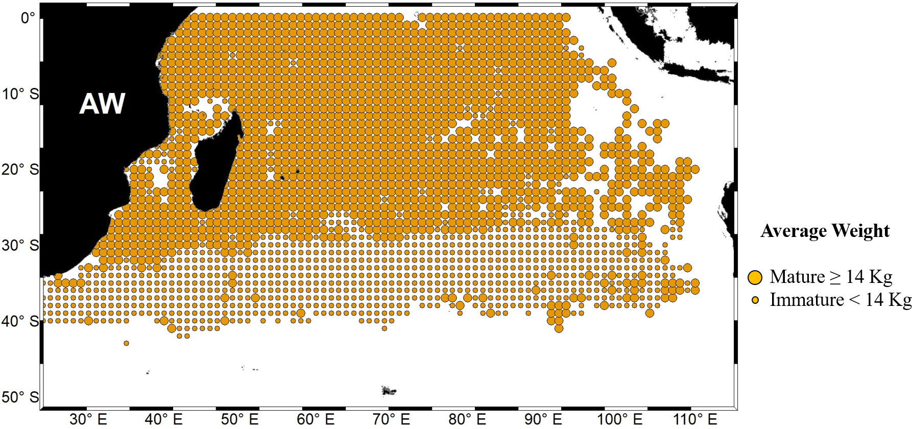
Figure 1 Weight distribution of mature albacore tuna in the Indian Ocean based on large-scale Taiwanese long-liner data from 1998 to 2016. AW indicates the average weight. Bigger and smaller circles indicate average weight of more or equal and less than 14 kg, respectively.

2.1.2 Oceanographic data

Data for the following ten oceanographic parameters were collected from various satellites (Table 1) and sources: SST, sea surface dissolved oxygen (OXY), sea surface salinity (SSS), MLD, SSH, sea surface zonal and meridional current (U, V), sea surface eddy kinetic energy (EKE), SSC (0–2 month lag), net primary productivity (NPP), rainfall (RF), and wind speed (SSW). These ten parameters are crucial for investigating albacore habitat patterns. SST regulates the body metabolism of albacore tuna. OXY is necessary for the maintenance of physiological processes. SSS is involved in marine species osmoregulation, and MLD and SSH are positively and negatively associated with SST, respectively. Ocean current speed is a key parameter for fast swimming fish such as tunas. SSC is important because it attracts secondary consumers, on which tuna feed. SSC productivity, the rate at which solar energy is captured in sugar molecules during photosynthesis (Lee et al., 2015), is an indicator of primary productivity. NPP, or the production of plant biomass, is equal to all of the carbon produced by vegetation through photosynthesis minus the carbon that is used for respiration (Lee et al., 2015); both SSC and NPP were considered in the present study. Finally, RF is inversely related to SST and was measured to investigate its potential effect on the distribution of mature albacore tuna. Spatial coverage of the data was from 0°S–45°S and 20°E–120°E with different spatial resolutions. All data collected from 1998–2016 for October to March correspond to the large-scale mature albacore tuna fishery data. Some of the environmental data were not available with spatial coverage of 1° × 1° and were interpolated to a 1° × 1° spatial grid because the spatial resolution of the fishery data was 1° × 1°; MATLAB version 2019a (Math Works, Natick, MA, USA) was used for this. All data were obtained on February 2, 2022.

1. MODIS = Moderate Resolution Imaging Spectroradiometer (https://www.ncei.noaa.gov/erddap/index.html).

2. COP = Copernicus (https://resources.marine.copernicus.eu/products).

3. AVISO = Archiving, Validation and Interpretation of Satellite Oceanographic data (https://coastwatch.pfeg.noaa.gov/erddap/griddap/erdTAssh1day.html).

TABLE 1

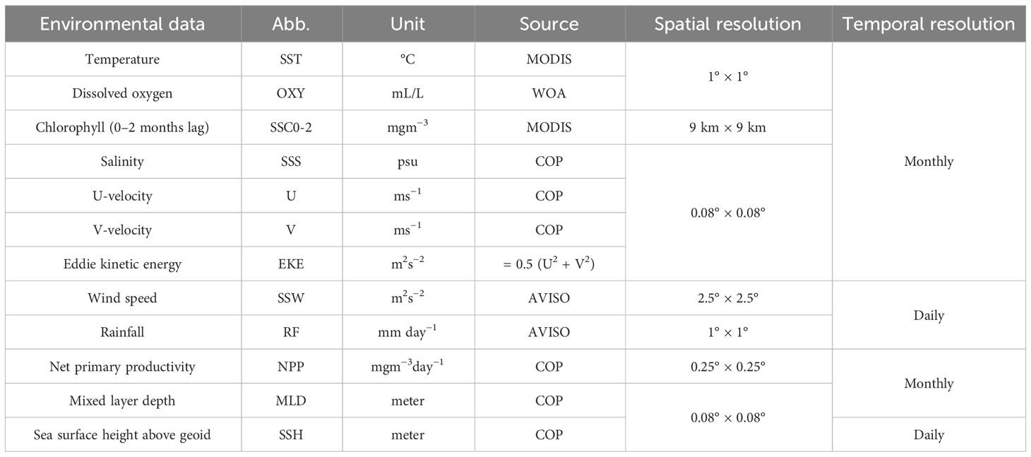
Table 1 Source of different oceanographic data.

EKE was calculated as EKE = 0.5 (U² + V²) m²s⁻².

A brief experimental flowchart is presented in Figure 2.

FIGURE 2

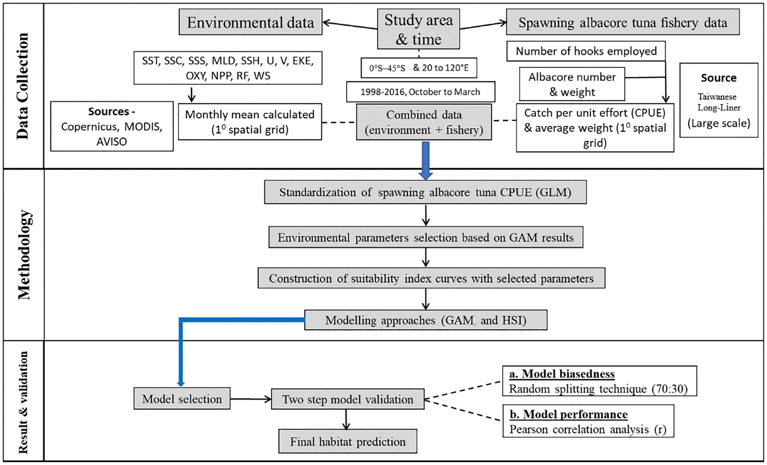
Figure 2 Experimental flowchart. Step by step methodology is illustrated.

2.2 Standardization of nominal CPUE

Mature albacore relative abundance was indexed as nominal CPUE (N.CPUE). N.CPUE (per 1000 hooks) was calculated using the following formula:

N. CPUE = \frac{N o . o f a l b a c o r e c a u g h t}{N o . o f h o o k s u s e d}

The standardization of CPUE is a crucial practice in the fields of fisheries and ecological research. The process of standardizing the CPUE entails making adjustments to the original CPUE values in order to mitigate any potential biases that could affect the outcomes (Mercer et al., 2023). To reduce the biased effects of various spatial (latitude, longitude) and temporal (year, month) factors, N.CPUE was standardized using a conventional method, GLM, to obtain bias filtered data (S.CPUE). Gear selectivity was not included in the standardization method as only long-line catch data were used in the present study. Consequently, vessel size was not included as information about vessel size for all the catches was unavailable. A stepwise GLM model (Lee et al., 2020; Vayghan et al., 2020; Mondal et al., 2021) was constructed with one to six factors in R studio version 3.6.0 using the mgcv package. In total, six models were compared and the optimal model was based on the lowest Akaike information criterion (AIC), the highest deviance explained (%), and the highest correlation (R²) values selected for standardization. The GLM models were constructed as follows.

G L M_{n} : L o g (N . C P U E + c) \sim a_{1} + a_{2} + a_{3} + …. a_{n} + µ + €

where c is a constant equal to 0.1, n is the number of variables, GLM_n refers to the model with n factors, µ is the intercept (Year × Lat, Year × Lon, and Lat × Lon), and € is a normally distributed variable with a mean of 0.

2.3 Environmental parameters selection for the model construction

GAM was used for parameter selection, and each parameter was ranked according to AIC and correlation (R²) value. Only the parameters that had correlation values of greater than 0.3 (a strong enough correlation per a shaky linear rule) were selected for model construction (Ratner, 2009). Collinearity among the selected parameters was assessed using R studio version 3.6.0. Correlation values greater than 0.6 (Chang et al., 2021) indicated collinearity among the parameter pairs.

2.4 Construction of suitability index curves

Suitability index (SI) curves were plotted for each selected parameter using summed mature albacore S.CPUE and smoothing spline regression to determine the relationship between mature albacore relative abundance (S.CPUE) and environmental variables (Lee et al., 2020; Vayghan et al., 2020; Mondal et al., 2021). In this analysis, S.CPUE was included as the dependent variable, and all selected environmental parameters were included as explanatory variables. The SI for mature albacore was established by applying S.CPUE and all environmental variables and was then normalized as follows (Austin, 2007).

S I = \frac{Y - Y m i n}{Y m a x - Y m i n}

where Y_max and Y_min, respectively, are the maximum and minimum number of observations of the S.CPUE or environmental variables, and Y is the simulated (predicted) value from Y_max to Y_min; thus, SI values can range only from 0 to 1.

The SI value was calculated using the summed frequency distribution of the S.CPUE of each class, and SI values were assumed to be between 0 and 1. The mid-points of each environmental variable class interval were used as observed values to fit the SI models. Finally, the relationship between the SI and environmental variables was calculated using the following formula (Chen et al., 2010; Lan et al., 2018).

S I = e^{α {(m + β)}^{2}}

where m denotes the response variable (environmental parameters), and α and β are fixed by applying the nonlinear least squares estimate to minimize the residuals between SI observation and SI function.

2.5 Approaches to habitat modeling

Conventional models, such as AMM and GMM and regression models, such as GAM, were used in this study. The main advantage of these types of models is their amenability to nonlinear prediction; these models thus realistically reflect the relationship between habitat preference (Mondal et al., 2021) and environmental factors. Thus, the habitat of mature albacore can be described easily based on environmental ranges. The simple AMM method algorithm yields the ratio of the sum of all observations to the total number of observations. The GMM method algorithm proceeds by multiplying all numbers and computing the nth root of these multiplicative products, where n is the total number of data points. The AMM and GMM algorithms are described using the following equations.

A M M_{n} : L o g (S . C P U E) \sim (a_{1} + a_{2} + a_{3} + …. + a_{n}) / n

G M M_{n} : L o g (S . C P U E) \sim {(a_{1} x a_{2} x a_{3} x …. x a_{n})}^{(1 / n)}

Where a₁, a₂, a₃ are different observations and n is the nth observation.

The GAM model was as follows.

G A M_{n} : L o g (S . C P U E) \sim s (a_{1}) + s (a_{2}) + s (a_{3}) + …. + s (a_{n})

where S.CPUE is the standardized CPUE of the long-line catch data, s is a smoothing function of each model covariate, and a_n is the nth oceanographic parameter.

2.6 Model selection and validation

One candidate model was chosen from each modelling method, namely conventional and regression, based on various indices, including Pearson correlation (R²) (with a preference for higher values; GAM, HSI) and AIC (with a preference for lower values; GAM, HSI). A total of two candidate models, one from the GAM and one from the HSI, were chosen for subsequent analysis.

Initially, the fishing dataset was partitioned into two random subsets, with a distribution ratio of 70% and 30%, respectively, utilizing the “Split” package and validation was conducted using the tidyverse and caret packages in R version 3.6.0. To assess the validity of the chosen GAM model, three coefficients were computed for both the training and testing datasets: R², RMSE (root mean square error), and MAE (mean absolute error). In order to validate the chosen model from HSI, only the R² was computed for both the training and testing datasets. Any model with the smallest discrepancies in R², RMSE, and MAE values between training and testing datasets, exhibited superior model performance characterized by reduced bias.

2.7 Prediction

The final two selected candidate models were then used for prediction if the validation method had better model performance with no significant bias. The predicted values for each point of the study area from the final model were then placed on a 1° × 1° spatial grid using ArcGIS software (version 10.2). The selected candidate model from GAM was used to predict CPUE (P.CPUE); this was used as a proxy for relative abundance. The selected candidate model from HSI was used to predict habitat suitability index (P.HSI) which indicated the suitable habitat zone in the range of 0-1.

3 Results

3.1 Standardization of nominal CPUE data

Among the stepwise GLM models constructed, the full GLM model (Model 5) had the lowest AIC value (184,070) and highest R² value (0.58; Table S1). The results on model performance in data standardization are depicted in Figure 3. The quantile–quantile (QQ) plot and histogram of the model (Figure S1) used for standardization exhibited an almost normal distribution. Therefore, the selected model was used for the standardization of mature albacore N.CPUE. The N.CPUE ranged from 0.1 to 2,700 individuals (monthly summed CPUE; Figure 3). After standardization was performed, the monthly summed CPUE decreased to within 0.1–1,700 individuals. The S.CPUE was used for the subsequent analyses for mature albacore tuna.

FIGURE 3

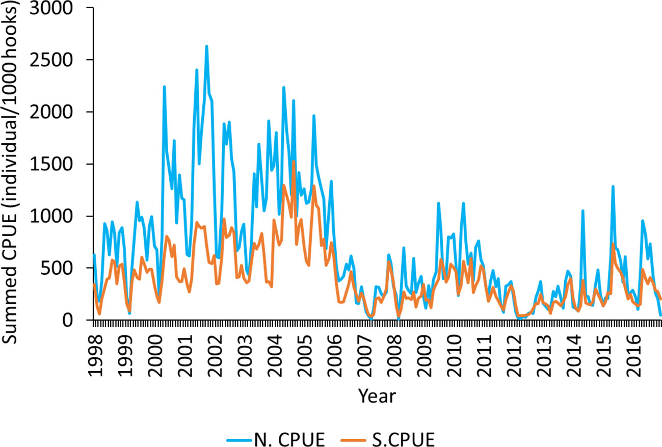
Figure 3 Nominal catch per unit effort (N.CPUE) and standardized catch per unit effort (S.CPUE) determined using the selected GLM model for mature albacore tuna.

3.2 Environmental parameter selection for model construction

Table 2 presents the environmental parameters obtained using different selection techniques. For the GAM method, OXY, SST, SSS, and SSH had correlation values greater than 0.3 in relation to S.CPUE; the correlation value for OXY was the largest at 0.793. The generalized cross-validation (GCV) index was also the lowest for OXY. Thus, only OXY, SST, SSS, and SSH were used for the final model construction. No collinearity was observed among the selected parameters (Table S2).

TABLE 2

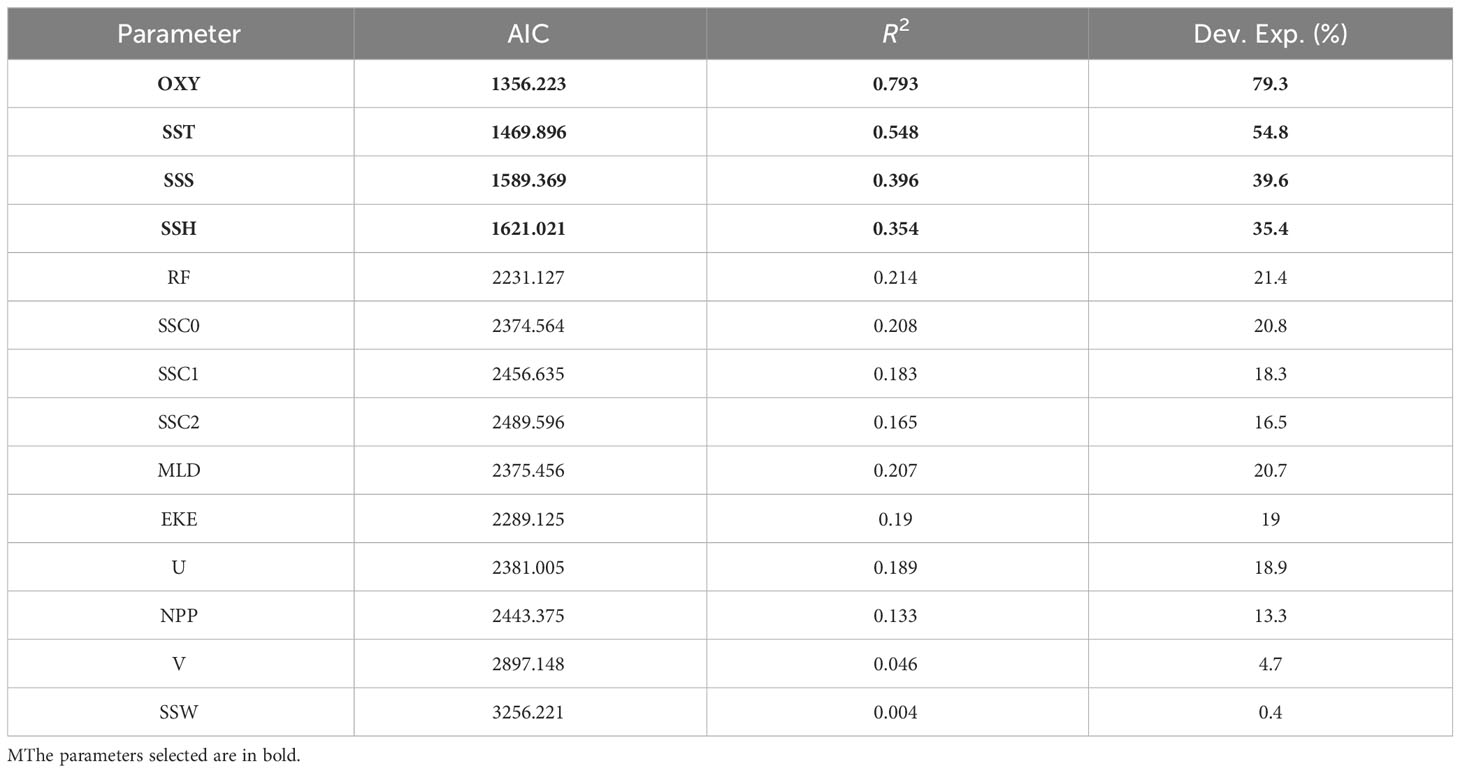
Table 2 Environmental parameter selection for model construction using GAM for mature albacore tuna.

3.3 Construction of SI curves

SI curves were constructed for mature albacore tuna against all the selected parameters (Figure 4), and the habitat SI was calculated. The optimal ranges of SST, SSS, OXY, and SSH were 25–29°C, 34.85–35.55 psu, 5–5.3 mL L⁻¹, and 0.5–0.7 m, respectively, at SI values >0.6. The sum of the S.CPUE of mature albacore in the Indian Ocean from October to March was around the SST, SSS, OXY, and SSH values of 27.5°C, 35.05 psu, 5.1 mL L⁻¹, and 0.55 m, respectively, at SI values >0.6 (Figure 4).

FIGURE 4

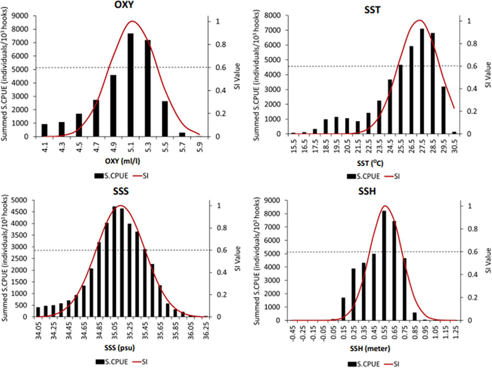
Figure 4 Suitability index (SI) curves of selected environmental variables for mature albacore tuna plotted using smoothing spline regression. Black bars, black dotted lines, and red solid lines indicate the summed standardized catch per unit effort (S.CPUE), SI with a cutoff value of >0.6, and SI curve, respectively. The intersection of the horizontal dotted line and SI curve indicates the optimal environmental range for each parameter.

3.4 Analysis of habitat model and model selection

Table S3A presents the performance results of the GAM models with all possible combinations of the selected parameters. Model 10 with OXY, SST, SSS, and SSH performed better than the other GAM models. It had the lowest AIC (80,008.57) and GCV (0.339) values with the highest adjusted R² (0.839) and percentage variance (83.9%).Thus, model 10 was selected as the optimal GAM model.

Table S3B presents the performances of AMM based HSI models with selected parameters in all possible combinations. Model 2 with OXY, and SSS indicated better performance than other AMM models. It indicated the lowest AIC value of 14.240 with the highest adjusted R² of 0.845. Thus, model 2 was selected as the optimal AMM model. Table S3B also indicated the performances of GMM based HSI models with selected parameters in all possible combinations. Model 7 with OXY, SST, and SSS indicated better performance than other GMM models. It indicated the lowest AIC value of 18.943 with the highest adjusted R² of 0.87. Thus, model 7 was selected as the optimal GMM model. After comparing the selected AMM and GMM model, the GMM based HSI model was determined to be optimal based on correlation values (Figure 5).

FIGURE 5

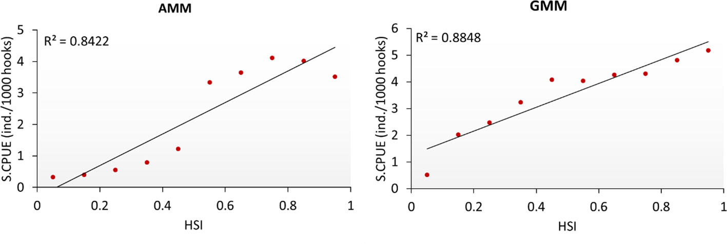
Figure 5 Comparison between the selected habitat suitability index models for mature albacore tuna.

3.5 Validation of the selected models and prediction

For GAM, results obtained using the random split validation technique indicated that the difference between the coefficient values (R², RMSE, and MAE) of the split datasets (70:30) were minimal; this entailed the absence of significant bias for the predictive performance of the selected GAM model (Table 3). Therefore, Model 10 of GAM was used for the final prediction of CPUE for all points of the study location. The selected HSI based habitat model also indicated that the difference between the R² of the split datasets (70:30) was minimal; this entailed the absence of significant bias for the predictive performance of the selected GMM model (Table 2). Therefore, Model 7 of GMM was used for final HSI prediction for all points of the study location.

TABLE 3

Table 3 Validation outcome selected models for mature albacore tuna before CPUE and HSI prediction.

In the month of October, the higher S.CPUE values had a scattered distribution (Figure 6). From November to January, higher mature albacore S.CPUE were primarily observed between 10°S–25°S. From February, a southward shift of S.CPUE towards areas below 30˚S could be observed which then became clearer in March with a high S.CPUE zone noted in areas along 35°S. Areas with lower S.CPUE values were mainly present towards north of 10°S of and south of 25°S throughout the study period. P.CPUE and P.HSI also followed a similar trend as S.CPUE with the higher observation approximately at 15°S–25°S (Figure 7) during the study period. Longitudinally, this area extended towards the east up to 100°E in the month of March. Based on P.HSI, suitable habitat zones were observed mainly between 10–25°S from October to March.

FIGURE 6

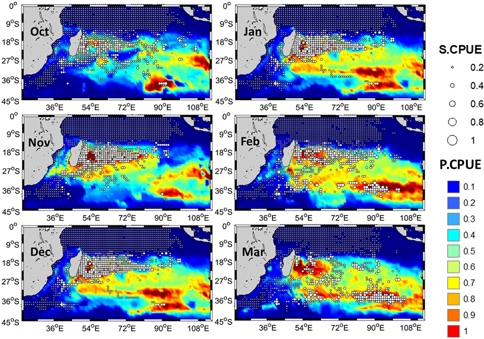
Figure 6 Monthly spatial distribution of the average standardized catch per unit effort (S.CPUE) of mature albacore tuna mapped on monthly predicted catch per unit effort (P.CPUE) in the Indian Ocean from 1998 to 2016.

FIGURE 7

Figure 7 Monthly spatial distribution of the average standardized catch per unit effort (S.CPUE) of mature albacore tuna mapped on monthly predicted habitat suitability index (P.HSI) in the Indian Ocean from 1998 to 2016.

4 Discussion

Management of the Indian Ocean albacore tuna fishery is crucial for future sustainability. Thus, practical tools must be used to enhance our understanding of key oceanographic parameters that affect albacore tuna distribution in the Indian Ocean. Based on the long-term Taiwanese fisheries long-line data, the study provides some key insights on the spatial distribution pattern of mature albacore tuna in the Indian Ocean and the influence of the marine environment on their distribution.

4.1 Environmental preferences

Environmental parameters are crucial for describing the distribution of any tuna species in the world’s oceans. Throughout the study period, mature albacore tuna tended to have a higher distribution in the 25–29°C range, particularly at 27.5°C in the Indian Ocean. This indicates the predominance of Indian Ocean mature albacore tuna in the warmer waters. One possible reason is that warmer water is suitable for spawning (Farley et al., 2013). SST is a significant environmental determinant that exerts influence on fish spawning, thereby impacting both the timing and success of this reproductive process. Additionally, SST during the spawning period affects the egg or larval development and survival of any species (Dhurmeea et al., 2016; Nikolic et al., 2017). Moreover, metabolism and reproduction are deeply connected to each other (Fontana and Della Torre, 2016). The acceleration of metabolic activity with increasing temperature suggests a slower metabolism in relatively cooler water. A sluggish metabolic rate can hinder the process and consequently reproduction. The influence of SST on the timing, success, and behaviors related to fish spawning is of utmost importance in the field of ocean studies. In addition, it exerts influence on various aspects such as egg development, larval survival, metabolic rates, mating rituals, and habitat. Furthermore, albacore may also remain in warm waters of the Indian Ocean to avoid being in direct competition for prey with juvenile albacore which tend to stay in cooler waters south of 30˚S in the Indian Ocean (Dhurmeea et al., 2016). Whilst the warm tropical waters of the Indian Ocean are oligotrophic, there are however regions of high productivity in specific areas (i.e. upwelling regions) at specific times of the year (Veldhuis et al., 1997). Thus, these factors may be the most plausible explanations for why mature albacore in the Indian Ocean were found to occupy warmer water in the current study. Mature albacore tuna in the Indian Ocean has also previously been found to have a SST range of 24–27°C during October to March (Chen et al., 2005), which supports the result of the present study.

Mature albacore tuna tended to have a higher distribution during the course of the study between 34.85 and 35.55 psu salinity, particularly around 35.05 psu in the Indian Ocean. The importance of SSS on albacore tuna distribution has been addressed in previous studies (Goñi et al., 2015; Novianto and Susilo, 2016). The effect of SSS on albacore tuna may be a proxy for other underlying processes (Mondal et al., 2022). Reglero et al. (2017)’s hypothesis, which proposed that salinity serves as an indirect predictor of oceanic conditions, provided evidence in favor of this assertion. Salinity may have an impact on a fish’s standard metabolic rate, food intake, food conversion, and endocrine regulation (Brett and Groves, 1979; Bœuf and Payan, 2001). Moreover, changes in sea surface salinity are directly connected with changes in water density (Biescas et al., 2014). The optimal density range will subsequently change as the preferred sea surface salinity range of any species changes. As water density falls outside of the preferred range, which results in energy loss, lower salinity can make swimming difficult (Bœuf and Payan, 2001). Increased salinity outside of the desired range might affect the cost of osmoregulatory regulation, requiring more energy (Urbina and Glover, 2015). Thus, salinity may have an impact on mature albacore distribution through habitat preference, with mature albacore being more common in areas with ideal salinity and less common in areas with more extreme salinity levels (Goñi et al., 2015). Proper salinity levels are essential for successful egg development, fertilization, larval survival, and the overall reproductive success of fish (Ruiz-Jarabo et al., 2022). Similarly, Chen et al. (2005) found that mature albacore tuna in the Indian Ocean have a SSS preference range of 35.01-35.32 psu, which supports the result of the present study.

Throughout the duration of the investigation, mature albacore tuna tended to have a higher distribution with OXY between 5-5.3 mL L^-1, particularly at around 5.1 mL^-1in the Indian Ocean. Oxygen intake naturally rises during swimming. Due to its high metabolism, albacore has a high oxygen requirement (Lehodey et al., 2015) with concentrations of at least 2 mL L^-1 generally required (Collette and Nauen, 1983). OXY levels can thus limit albacore tuna vertical distribution (Wang et al., 2023). The present investigation revealed a greater OXY range, which may be explained by the mature albacore tuna’s demand for higher metabolic activity during spawning (Karamushko and Christiansen, 2002). In addition, an optimal rate can result in greater food conversion and enhance larval or juvenile growth (Mallya, 2007). Moreover, decreased oxygen levels outside of the desired range can cause behavioral alterations such as shifts in horizontal or vertical distribution, adjustments to swimming activity, or breathing issues (Brill, 1994). More stress is indicated by a low concentration of OXY from the preferred value. OXY level below 2 mL L-1 can result in mortality of fish (Keller et al., 2015). The area with higher distribution in the present study has higher concentration of OXY. The presence of multiple ocean currents, such as the South Equatorial Current, South Indian Ocean Countercurrent, Madagascar Current, and Agulhas Current, contributes to this phenomenon. Ocean currents in this region facilitate the thorough mixing and ventilation of water through the upwelling process. This phenomenon impacts the mixing and transportation of oxygen-rich waters, forming oxygen-rich areas and affecting the overall biological productivity of mature albacore in the study area (McCreary et al., 2013). Mature albacore tuna in the Indian Ocean has an OXY preference range of 5.09-5.75 mL L-1, according to Chen et al. (2005), which supports the result of the present study.

4.2 Spatial distribution pattern

During October, high S.CPUE regions were distributed in a scattered manner. From November to January, higher mature albacore distribution was mainly observed between 10°S–25°S. From February, a southward shift was observed, and a higher mature albacore distribution zone was observed at approximately 35°S. In March, this shift was clearer. During March, P.HSI does not show the peak in values at around 35°S, whereas the P.CPUE does show high values in this more temperate zone. HSI represents the habitat suitability, whereas CPUE represents the relative abundance. Mature albacore tuna showed a southward shift after February and so a significant abundance near 35°S though habitat was still suitable for mature albacore near 18-25°S. The habitat suitability may be impacted by the life cycle of albacore tuna, that is, the tropical area between 10-25˚S is suitable mainly for spawning, especially during November to January, while the temperate areas (35˚S) are mainly for foraging by juvenile and adult albacore after the spawning season (Dhurmeea et al., 2016). The temperate waters of the Indian Ocean are considerably cooler than the tropical and subtropical waters, which can be favorable for the higher prey concentration (Chen et al., 2005). Cooler waters can promote the growth of greater phytoplankton blooms than warmer waters (O’Dowd et al., 2015). Increased nutrient availability and favorable light conditions for photosynthesis can cause these blooms (Trombetta et al., 2019). The abundance of phytoplankton can attract herbivorous zooplankton, thereby increasing the concentration of prey for predatory fish such as tunas. This is one plausible explanation for why mature albacore tuna shifted southward in temperate waters even though the models indicated favorable habitat suitability at 18-25°S. Mature albacore tuna spatial distribution patterns can be attributed to several possible reasons. The first one is the presence of preferred optimal environmental ranges. A 27.5°C SST isotherm line’s presence can be linked to the distribution pattern of mature albacore in the Indian Ocean. Between October and March, a southward shift in the direction of the 27.5°C SST isotherm line was seen (Figure 8). The monthly movement of the aforementioned isotherm line may thus be one explanation for the shift in mature albacore tuna spatial distribution. The relationship between the adult albacore tuna’s geographical distribution pattern and environmental factors like SSS and OXY can be explained by the SST. SST was negatively correlated to both SSS and OXY. Hence, the spatial location of the ideal SSS and OXY will also be impacted by the 27.5°C SST isotherm line’s migration southward. The distribution range of mature albacore tuna is expected to undergo a spatial shift due to alterations in the optimal SST zone.

FIGURE 8

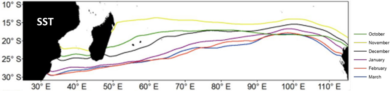
Figure 8 Locations of 27.5°C SST isotherm during the study months.

Because subtropical gyres between 10–30°S move water, salinity, and nutrients essential to marine ecosystems over great distances (Visser et al., 2015), they may also play a significant role in the high quantity of mature albacore tuna (Romanov et al., 2020) in the area from October to March. On Madagascar’s south-east coast (especially, 16°S–22°S, and 52°E–90°E), the subtropical gyre induces upwelling, which raises the productivity of the oceanic zone there (Romanov et al., 2020) and creates favorable conditions for mature albacore tuna. However, the Indian Ocean subtropical gyre is typically associated with low upwelling compared to some other oceanic regions (Visser et al., 2015; Chinni and Singh, 2022). Distribution of albacore tuna can be still higher in this region, because this kind of water exhibits less competition (due to limited nutrients) for mature albacore with other species due to spawning purposes as explained above. Spawning in less productive waters may be a strategy used to reduce the risk of predation of eggs and larvae by pelagic predators which are usually abundant in high productivity areas (Johannes, 1978). In addition, it is commonly observed that oligotrophic sub-tropical gyres exhibit a strong correlation with expansive oceanic currents. The currents above can effectively transport a wide range of substances, including nutrients, food particles, and larvae, across extensive distances. The reallocation of resources can enhance food availability and support the development of albacore larvae. A minor amount of mature albacore tuna may still remain in the area between 10-30˚S for foraging purposes outside the spawning season (i.e. the study period).

The final cause can be the influence of fishing activity on S.CPUE. From October to March, the S.CPUE was between 10°S–30°S (Figure 9). A strong correlation was observed between N.CPUE and the number of hooks; the correlation value was 0.632 for mature albacore tuna. A strong correlation was also observed between N.CPUE and albacore quantity; the correlation value was 0.621 (mature from October to March). This strongly implied that S.CPUE was affected by fishing activity.

FIGURE 9

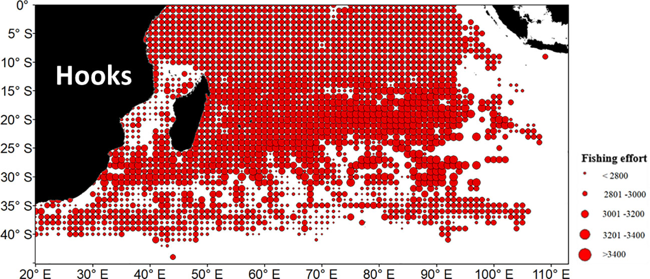
Figure 9 Average fishing effort (number of hooks) based on the mature albacore tuna data from October to March.

4.3 Potential implications for albacore fisheries

The primary objective of this study was to contribute to a toolkit for policymakers and managers who are considering climate adaptation for marine fisheries management. Habitat models can facilitate the search for productive fishing locations or new fishing grounds, saving time, money, and fuel. Nonetheless, the potential ease of overfishing as a result of the increased accessibility of fishing areas highlights the critical importance of sustainable development goals (SDGs). The SDGs aim to address ocean health issues such as overfishing and global warming. Understanding the distribution of mature albacore tuna in the Indian Ocean can facilitate long-term care and conservation initiatives. SDG 14.4 aims to maintain biologically sustainable fish stocks, whereas SDG 14.5 protects coastal and marine environments. After understanding the current status of habitats or identifying new fishing grounds, achieving these SDGs is straightforward. Modeling the locations or habitats of species can therefore be the first step in sustainability research. To maintain biologically appropriate levels of this species, it is essential to comprehend spatial and environmental habitat preferences of mature albacore tuna. The results of this study have the potential to develop adaptation techniques for the management of albacore tuna fisheries in the Indian Ocean and other oceans as well.

4.4 Study limitations and future research directions

Although the findings of this study are valuable for resource management and strategy evaluation, the present study also has limitations. Results on the habitat preferences of mature albacore could also be affected by the species habitat model algorithm and vertical behavior. Adopting various advanced habitat model techniques, assembling longer time-series fisheries data, and using available vertical oceanographic data can yield more robust insights into how mature albacore respond to various environmental factors. Moreover, the study is based solely on the catch of Taiwanese longliners and the areas of the Indian Ocean covered by these vessels. Future studies should aim to incorporate available albacore fisheries data from vessels from other countries and to also examine the effects of vertical changes in the environment on mature albacore distribution.

5 Conclusion

This study employed two empirical HSI models (AMM & GMM) and GAM model to describe the distribution of mature albacore tuna in the Indian Ocean during their spawning season (October to March). Higher mature albacore abundance was primarily observed from October to December. For the mature albacore tuna from October to March, the optimal ranges of temperature, salinity, oxygen, and SSH were 25–29°C, 34.85–35.55 psu, 5–5.3 mL L⁻¹, and 0.5–0.7 m, respectively. Mature albacore tuna tended to remain between 10–30°S from October to March. The suitable habitat zone for the mature albacore tuna from October to March was identified mainly at 15°S–25°S.

Data availability statement

The raw data supporting the conclusions of this article will be made available by the authors, without undue reservation.

Author contributions

SM: Conceptualization, Data curation, Formal Analysis, Methodology, Software, Validation, Writing – original draft, Writing – review & editing. ML: Conceptualization, Funding acquisition, Methodology, Project administration, Resources, Supervision, Validation, Visualization, Writing – review & editing.

Funding

The authors declare financial support was received for the research, authorship, and/or publication of this article. This study was funded by National Science & Technology Council (MOST111-2923-M-019-MY2).

Acknowledgments

We thank the two reviewers and the editor for their valuable comments and suggestions as well as the team members of the Fisheries Agency and Overseas Fisheries Development Council of Taiwan for their assistance in data preparation. We also acknowledge Wallace Academic Editing Company for editing the manuscript.

Conflict of interest

The authors declare that the research was conducted in the absence of any commercial or financial relationships that could be construed as a potential conflict of interest.

Publisher’s note

All claims expressed in this article are solely those of the authors and do not necessarily represent those of their affiliated organizations, or those of the publisher, the editors and the reviewers. Any product that may be evaluated in this article, or claim that may be made by its manufacturer, is not guaranteed or endorsed by the publisher.

Supplementary material

The Supplementary Material for this article can be found online at: https://www.frontiersin.org/articles/10.3389/fmars.2023.1258535/full#supplementary-material

References

Arrizabalaga H., Dufour F., Kell L., Merino G., Ibaibarriaga L., Chust G., et al. (2015). Global habitat preferences of commercially valuable tuna. Deep Sea Res. Part II: Topical Stud. Oceanography 113, 102–112. doi: 10.1016/j.dsr2.2014.07.001