 Bayoumy Mohamed
 Alexander Barth
 Aida Alvera-Azcárate1
95% of researchers rate our articles as excellent or good
Learn more about the work of our research integrity team to safeguard the quality of each article we publish.
Find out more
ORIGINAL RESEARCH article
Front. Mar. Sci. , 19 September 2023
Sec. Physical Oceanography
Volume 10 - 2023 | https://doi.org/10.3389/fmars.2023.1258117
In this study, we examined the long-term spatiotemporal trend of marine heatwaves (MHW) and marine cold spells (MCS) characteristics in the southern North Sea over the last four decades (1982-2021). We then estimated the difference between their annual mean values and the possible relationship with the large-scale climate modes of natural sea surface temperature (SST) and atmospheric variability using satellite SST data. The SST warming rate was 0.33 ± 0.06°C/decade and was associated with an increase in MHW frequency (0.85 ± 0.39 events/decade) and a decrease in MCS frequency (-0.92 ± 0.40 events/decade) over the entire period. We found a distinct difference between the annual mean values of MHW and MCS characteristics, with a rapid increase in total MHW days (14.36 ± 8.16 days/decade), whereas MCS showed an opposite trend (-16.54 ± 9.06 days/decade). The highest MHW frequency was observed in the last two decades, especially in 2014 (8 events), 2020 (5 events), and 2007 (4 events), which were also the warmest years during the study period. Only two years (2010 and 2013) in the last two decades had higher MCS frequency, which was attributed to the strong negative phase of the North Atlantic Oscillation (NAO). Our results also show that on the annual scale, both the East Atlantic Pattern (EAP) and the Atlantic Multidecadal Oscillation (AMO) play a more important role in the formation of the MHW in the southern North Sea than the other teleconnections (e.g., the NAO). However, the NAO made the largest contribution only in the winter. Strong significant (p < 0.05) positive/negative correlations were found between oceanic and atmospheric temperatures and the frequency of MHW/MCS. This suggests that with global warming, we can expect an increase/decrease in MHW/MCS occurrences in the future.
Global mean sea surface temperature (SST) has increased in recent decades due to anthropogenic-induced climate change (IPCC, 2021). One of the most certain consequences of this global warming is extremely warm ocean temperatures, known as marine heatwaves (MHWs) (Hobday et al., 2016). Due to the destructive impacts of MHWs on marine ecosystems, biodiversity, and fisheries, most of the previous studies have focused on MHWs at regional and global scales (Selig et al., 2010; Mills et al., 2013; Frölicher and Laufkötter, 2018; Smale et al., 2019; Sen Gupta et al., 2020). The other extreme cold-water phenomena, known as marine cold-spells (MCSs) have received little attention (Schlegel et al., 2021a; Wang et al., 2022), although MCSs also have crucial negative impacts on the marine ecosystem, such as shifts in the geographic distribution of marine species, mass mortality, and coral bleaching (Schlegel et al., 2017; Tuckett and Wernberg, 2018; Yao and Wang, 2022), As a result of anthropogenic global warming, the frequency and duration of MHW have increased globally over the last four decades (Oliver et al., 2018; Yao et al., 2022), while MCS generally decreased (Schlegel et al., 2021a; Wang et al., 2022). Because MHWs are driven by long-term SST warming rather than SST variability (Oliver, 2019), MHWs are expected to become more frequent and intense over the next century (Frölicher et al., 2018; Oliver et al., 2019). Recently, Mohamed et al. (2022b) found that these MHW events have extended to the Arctic seas (e.g., the Barents Sea) and are becoming more frequent, especially after the amplification of SST warming in the Arctic Ocean that occurred after 2004.
Numerous recent studies have focused on the causes and impacts of MHWs at regional to global scales, from the surface to the subsurface (Frölicher et al., 2018; Holbrook et al., 2019; Roberts et al., 2019; Sen Gupta et al., 2020; Smith et al., 2021; Schlegel et al., 2021b; Yao et al., 2022; Aboelkhair et al., 2023; Smith et al., 2023). The main ecological consequences of these extreme MHWs are their disturbance effects on foundation marine species (e.g., corals, seagrasses, and kelp forests) (Holbrook et al., 2020), benthic mass mortality (Garrabou et al., 2009), harmful algal blooms (Trainer et al., 2020), reduced surface chlorophyll levels (Bond et al., 2015; Hamdeno et al., 2022; Hamdeno and Alvera-Azcaráte, 2023), and changes in species behavior and fishing practices (Mills et al., 2013; Smale et al., 2019). MHWs are triggered by an interplay of regional atmospheric and oceanic processes and can be influenced by teleconnections and other large-scale climate variability (Holbrook et al., 2019; Holbrook et al., 2020). These processes include the persistence of a high-pressure system combined with reduced cloud cover over the ocean (i.e., atmospheric blocking), which can increase solar radiation and enhance heat transfer to the ocean. Weaker winds at the ocean surface and slower vertical mixing in the upper ocean can retain more heat at the ocean surface (Chen et al., 2015; Holbrook et al., 2019; Holbrook et al., 2020). In addition, enhanced horizontal heat advection by ocean currents and reduced coastal upwelling or Ekman pumping can increase local SST (Oliver et al., 2017; Holbrook et al., 2019).
The most influential large-scale climate modes of SST and atmospheric variability in the North Atlantic and European regions are the North Atlantic Oscillation (NAO), the East Atlantic Pattern (EAP), and the Atlantic Multidecadal Oscillation (AMO) (Hurrell et al., 2003; Knight et al., 2005; Trenberth and Shea, 2006; Scannell et al., 2016; Mohamed et al., 2022a; van der Molen and Pätsch, 2022). These climate modes are associated with changes in SST at interannual time scales (e.g., NAO) and on time scales of decades and longer (e.g., AMO and EAP) and can influence the likelihood of a MHW in this region. Several studies suggest that the genesis of MHW in the North Atlantic was strongly associated with these large-scale climate modes (Holbrook et al., 2019). For example, the most intense and prolonged MHW that occurred in the Northwest Atlantic in 2012 and severely impacted fisheries in that region (Mills et al., 2013), was primarily caused by local atmospheric warming that was enhanced by anomalous northward movement of the jet stream (Chen et al., 2014; Chen et al., 2015). This MHW began with a strong positive NAO phase in late 2011 (Chen et al., 2014; Chen et al., 2015), and the positive AMO conditions during the whole year increased the likelihood of MHW in the northwest Atlantic in 2012 (Scannell et al., 2016). Scannell et al. (2016) also found that MHW frequency in the North Atlantic was more strongly modulated by the AMO than by the NAO.
The North Sea is projected to warm twice as fast as global levels (Hobday and Pecl, 2014; Smale et al., 2019) and is strongly affected by extreme meteorological events (Chen et al., 2022). For example, the extreme atmospheric heatwaves of summer 2018 (from mid-July to early August 2018), which hit northwestern Europe with record-breaking air temperatures, were observed in many countries in this region (Kueh and Lin, 2020). During this event, dissolved methane concentrations in seawater along the Belgian coast were three times higher than normal concentrations at this time of year (Borges et al., 2019). The North Sea is also considered one of the most productive fisheries in Europe (Guiet et al., 2019) and a large marine ecosystem (Ducrotoy et al., 2000). The SST changes in this region had profound impacts on biological systems (Kirby et al., 2007) and resulted in significant economic consequences (e.g., for fisheries). However, few studies have focused on investigating SST extremes and their consequences in this region (Chen et al., 2022). To the best of our knowledge, there are no published studies that have examined the characteristics of MHW and MCS and their effects in the North Sea.
In this study, 40 years (1982-2021) of satellite-based SST data and ERA5 reanalysis of atmospheric variables (e.g., air temperature, air pressure, zonal and meridional wind components) over the southern North Sea were used to investigate: (1) the occurrence and classification of marine heatwaves (MHWs) and cold-spells (MCSs) and the spatiotemporal evolution and long-term changes in their main metrics (frequency, total days, and maximum intensity); (2) the local differences in the mean and trend between the MHW and MCS metrics; (3) the relationships between MHW/MCS frequency and the large-scale climate modes of natural SST and atmospheric variability (e.g., AMO, NAO, and EAP); (4) the atmospheric conditions during the two case studies of MCS in 2013 and MHW in 2014 that occurred in the last decade.
The North Sea is a marginal sea in northwestern Europe that connects the Baltic Sea to the Atlantic Ocean via the Norwegian Sea in the north and the English Channel in the southwest. This study focuses on the southern North Sea, a shallow water basin bordered by the United Kingdom (UK) to the west and the coasts of Germany and the Netherlands to the east, Belgium, and France to the south. The southern North Sea is defined as the area between 0-9°E longitude and 50-55°N latitude (Figure 1), connected to the Atlantic Ocean by the English Channel and the Strait of Dover. The average depth of the southern North Sea is about 25 m, with a maximum depth of about 50 m in the north and south of the United Kingdom and the shallowest depth (20 m) on Dogger Bank in the north. The southern North Sea is strongly influenced by the inflow of warm Atlantic water (AW) from the southwest through the English Channel (Figure 2A). This warm and salty AW flows further northward into the North Sea and influences the climate in the region.
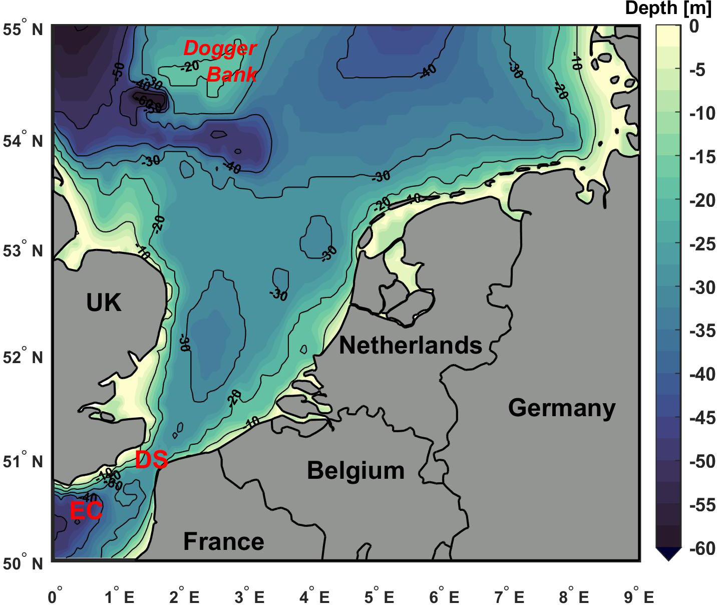
Figure 1 Bathymetry (source: GEBCO, https://www.gebco.net) of the Southern North Sea with the main geographical features. Isobaths of 10, 20, 30, 40, and 50 m are shown in black. The abbreviations stand for the English Channel (EC) and Dover Strait (DS).
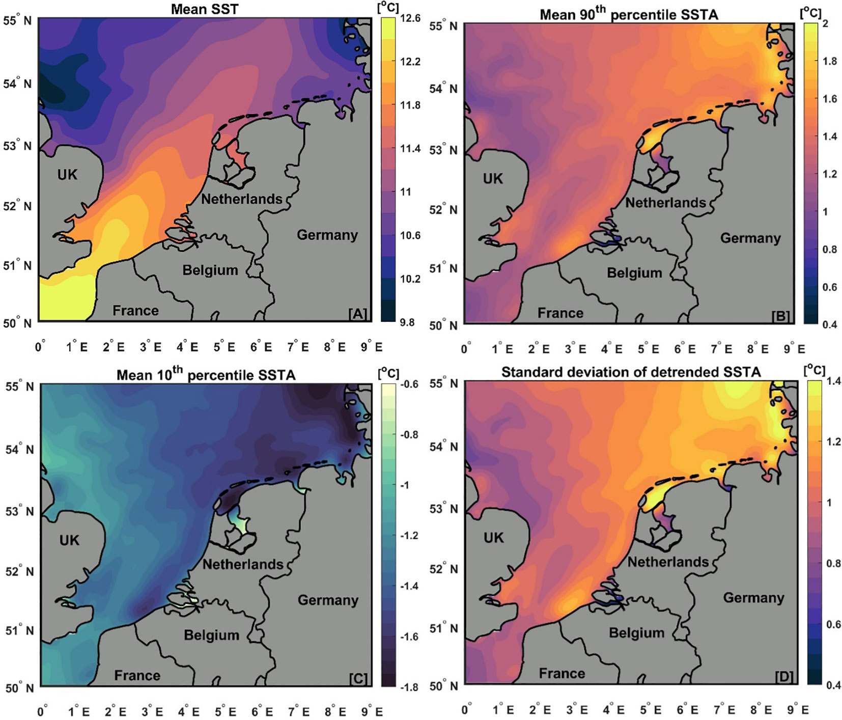
Figure 2 Spatial distribution of climatological daily mean (1982–2021) of (A) SST, (B) the 90th percentile of SSTA, (C) the 10th percentile of SSTA, and (D) standard deviation of detrended SSTA at each grid cell in the southern North Sea.
To detect MHW and MCS and their characteristics, we use high-resolution (0.05° × 0.05°) daily gridded SST data obtained from the Copernicus Marine Environment Monitoring Service (CMEMS; https://doi.org/10.48670/moi-00168, last accessed: 15 May 2023). This product was created from multiple satellite sensors and in situ observations by the Operational Sea Surface Temperature and Sea Ice Analysis (OSTIA; Good et al., 2020). The southern North Sea SST data were extracted from this global dataset, which covers a period of 14,610 days (from 1 January 1982 to 31 December 2021) and 9828 regular grid points.
To better understand the relationship between MHW/MCS and atmospheric conditions, we use the hourly gridded (0.25°x0.25°) atmospheric variables from the European Centre for Medium-Range Weather Forecasts (ECMWF) fifth-generation ERA5 reanalysis dataset (Hersbach et al., 2020). ERA5 provides hourly estimates for many atmospheric and oceanic variables from 1979 to the present. Variables used here include the daily mean surface air temperature (SAT), 10-m wind components (u10 and v10) and mean sea-level pressure (MSLP) from 1982 to 2021. Finally, the normalized monthly average time series of three of the large-scale teleconnection patterns, the NAO, the EAP, and the AMO, are obtained from the NOAA Climate Prediction Center (CPC https://www.cpc.ncep.noaa.gov/data/teledoc/telecontents.shtml; https://psl.noaa.gov/data/timeseries/AMO/, accessed on 5 April 2023).
In this study, MHWs and MCSs were determined according to the standard method outlined in Hobday et al. (2016) and (Schlegel et al., 2021a). Therein, MHWs (MCSs) are defined as “an unusually warm (cold) water event lasting at least five consecutive days with SST above (below) the seasonally varying 90th (10th) percentile threshold for that time of year”. The baseline climatology should be based on 30 years or more (Hobday et al., 2016). Here, the baseline climatology and thresholds for MHW and MCS are calculated for each grid cell for each calendar day of the year using daily SST data over the entire study period (1982-2021). When two consecutive MHW or MCS events occur with less than 2 days gap, they are considered a single event (Hobday et al., 2016). The use of these seasonally varying thresholds and baseline climatology allows the detection of MHW and MCS events at any time of the year, not just during the warm or cold seasons, whereas fixed thresholds (e.g., Frölicher et al., 2018) typically detect only MHW during the warm season and MCS during the cold season.
We used the MATLAB Marine Heatwaves (M_MHW) toolbox created by Zhao and Marin (2019) based on (Hobday et al., 2016) to detect all MHW and MCS characteristics. This implementation code is also publicly available in Python and R (Hobday et al., 2016; Schlegel and Smit, 2018), which are functionally identical to MATLAB (Hobday et al., 2016; Zhao and Marin, 2019; Pastor and Khodayar, 2023). Once the MHW/MCS events are detected, three indices are used in this study to represent the MHW/MCS characteristics, namely MHW/MCS frequency (the number of MHW or MCS events in each year), MHW/MCS days (the total number of MHW or MCS days in each year), and MHW/MCS maximum intensity (the highest SST anomalies occurring within all MHWs or MCSs in each year). The daily SST anomalies (SSTAs) were calculated with respect to the seasonal climatology for each grid cell. This is done by subtracting from the SST of each calendar day (e.g., January 1, 1982) the mean SST of that day (January 1) over the entire study period (1982-2021). The least squares method (Wilks, 2011) and the Modified Mann–Kendall (MMK) test (Hamed and Ramachandra Rao, 1998; Wang et al., 2020) are used to estimate the linear trends of SSTA and MHW/MCS characteristics (frequency, total days, and maximum intensity) and their statistical significance at the 95% confidence level.
To quantify the role of essential climate variables and large-scale climate indices on the observed MHW and MCS, we examined the relationship between MHW/MCS frequency and total days with the following climate variables and indices: SST, SAT, AMO, EAP, and NAO at the annual and seasonal scales. In shallow water regions such as the southern North Sea, the evolution of vertical thermal stratification is associated with the seasonal cycle of water temperatures (Chen et al., 2022). Therefore, in this study, we define three months with higher SST mean values (July–August–September) as summer and those with lower SST mean values (January–February–March) as winter. In addition, a spatial correlation and composite analysis were performed between MHW/MCS frequency and the three selected large-scale climate modes (AMO, NAO, and EAP) to investigate their possible role in forcing MHW and MCS in the southern North Sea. The positive and negative phases of each climate mode are defined when their values are higher or lower than one standard deviation from their climatological mean (1982–2021) (Sandler and Harnik, 2020; Mohamed et al., 2022b).
The regional climatological mean SST over the southern North Sea, 90th percentile SSTA, 10th percentile SSTA, and standard deviations of detrended SSTA from 1982 to 2021 are shown in Figures 2A–D. The southern North Sea is characterized by a lower climatological SST mean (< 10.6°C) in the northwestern part and in the German Bight (Figure 2A), compared to the southern part of the basin, which has a higher climatological SST mean (> 12.2°C), possibly due to the inflow of warm Atlantic water through the English Channel and Dover Strait (Ducrotoy et al., 2000). After subtracting annual cycles, the 90th percentile SSTA from 1982 to 2021 was generally above 1.4°C in most of the southern North Sea, with the highest values (up to 2°C) in the northeastern part and along the Dutch coast and the German Bight (Figure 2B). The lowest values (<1.4°C) were recorded along the British coasts. The 10th percentile SSTA shows an opposite pattern with the highest negative values in the northeastern part (Figure 2C). The 10th percentile threshold anomaly values are generally about -0.6 to -1.8°C below the seasonal climatological mean (Figure 2C). Figure 2D shows the spatial pattern of the standard deviations of detrended SSTA over the entire study period. These standard deviation values allow us to assess the overall SST variability that is not explained by the seasonal cycle and linear trends. The highest standard deviations (> 1.2°C) are observed in the northeastern part of the North Sea and the German Bight (Figure 2D). The region of the AW inflow has the lowest standard deviations (0.4-0.8°C). In general, the 90th percentile, standard deviation, and 10th percentile of the SSTA show zonal (west-east) variation, with the highest values in the east for both the 90th percentile and standard deviation and the lowest values for the 10th percentile.
From the analysis of SST anomalies (Figures 3, S1B), it is evident that there is a strong temporal evolution of the regionally averaged SSTA in the southern North Sea from 1982 to 2021. Between 1982 and 1997, the southern North Sea shows predominantly negative SSTA, except for 1989/1990 and 1995, which show positive SSTA during this period. From 1998 onward, overall positive SSTAs predominated, except in the winters of some years (e.g., 2006, 2009-2013, and 2018) negative SSTAs were observed. These negative SSTAs were associated with a strong negative phase of the NAO index (see Figure S2A). The reversal of SST from negative to positive anomalies coincides with the AMO inversion from negative to positive phase in 1998 (see the red line in Figure 3). The AMO index is strongly correlated (R= 0.6) with SSTA in the North Sea on the interannual time scale (i.e., 12-month mean). In general, 2007, 2014, and 2020 were the warmest years during the study period, with SSTAs of 1.5°C above the climatological mean (1982-2021). The years 1985-1987, 1996, 2011, and 2013 were the coldest years during the study period, as the SSTA was less than 1.5°C below the climatological mean (1982-2021). The overall temporal trend of SSTA is about 0.33 ± 0.06°C/decade (the solid black line in Figure 3). This result is consistent with Tinker and Howes (2020).
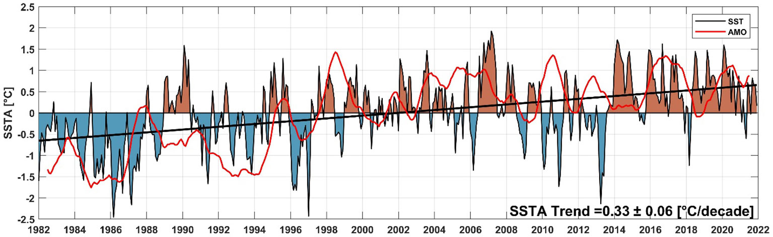
Figure 3 Southern North Sea averaged sea surface temperature anomaly (SSTA) and Atlantic Multidecadal Oscillation (AMO) index from 1982 to 2021. The red/blue shaded regions represent positive/negative SSTA, respectively. The black line represents the temporal linear SSTA trend (°C/decade). The red line is the normalized AMO index smoothed with a12-month window.
The spatial distribution of the warming SSTA trend is statistically significant (p < 0.05) over the entire southern North Sea from 1982 to 2021 (Figure 4). However, this trend is not uniform over the whole region and exhibits high spatial variability, ranging from 0.1 to 0.5°C/decade. The highest SST trend is observed in the central and northeastern parts of the study region. This could be attributed to the increased inflow of warm Atlantic water. The lowest SST trend is found along the northern Dutch coast and in the German Bight, where cold freshwater inflows occur (Ducrotoy et al., 2000).
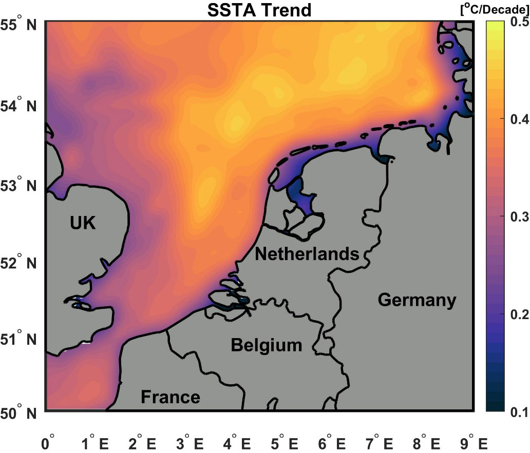
Figure 4 Spatial trend (°C/decade) map of SSTA over the southern North Sea from 1982 to 2021. Note that the SSTA trends are statistically significant (p < 0.05) at the 95% confidence level over the whole region.
The mean annual characteristics of MHW and MCS between 1982 and 2021, such as annual days and maximum intensity, and the difference between these characteristics over the southern North Sea are shown in Figure 5. Mean annual MHW and MCS days exhibit high spatial variability (Figures 5A, C), but this variability is not systematic (Figure 5E). High mean annual MHW days (more than 30 days) are observed in the region between the United Kingdom and Belgium and in the northern Netherlands and in the German Bight. The lowest values of MHW days (20-24 days) are found in the English Channel and northwestern regions (Figure 5A). A higher number of MCS days is found in most of the study area (Figure 5C), except for the northern coasts of the Netherlands and Germany (i.e., the same region that shows a lower SST trend, see Figure 3).
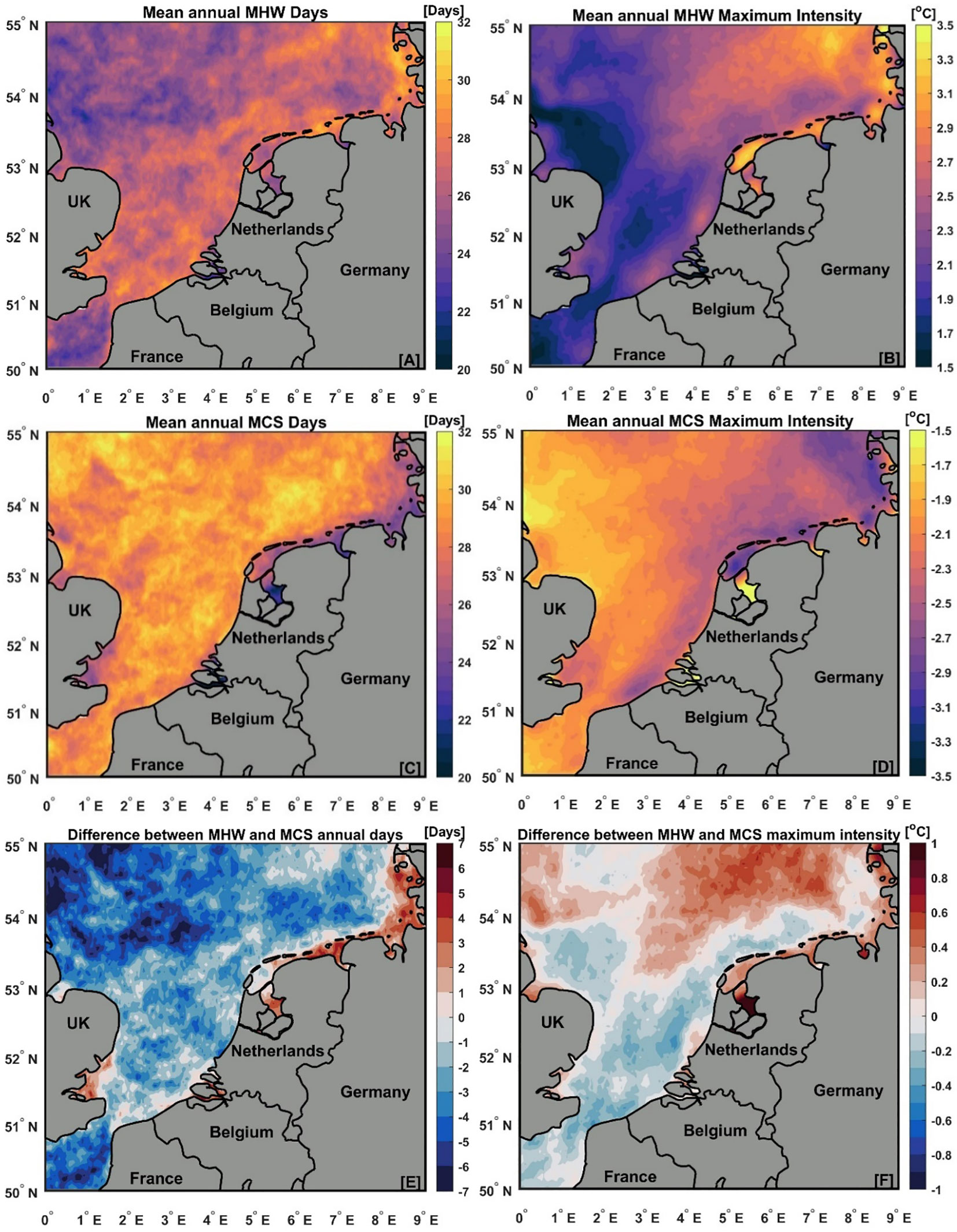
Figure 5 Spatial distribution of annual mean values of the total number of days and the maximum intensity of marine heatwaves (MHW) and marine cold-spells (MCS) and the differences between them in the southern North Sea from 1982 to 2021, (A) MHW days (days), (B) MHW maximum intensity (°C), (C) MCS days (days), (D) MCS maximum intensity (°C), (E) the difference between the mean annual MHW days and the mean annual MCS days (i.e., (A) minus (C)), and (F) the difference between the mean MHW maximum intensity and the mean MCS maximum intensity (i.e., (B) plus (D)). For (E, F), positive values (red areas) indicate that annual MHW days are greater than annual MCS days and MHW maximum intensities are more intense than MCS maximum intensities. The opposite is true for the negative values (blue areas).
The maximum intensity of MHW and MCS is greatest along the northern Dutch coast and in the German Bight (Figures 5B, D). The spatial pattern of MHW maximum intensity exhibits a dipolar or zonally increasing gradient from west to east (Figure 5B). The most intense MHWs, in terms of maximum intensity, are in the eastern part of the southern North Sea (i.e., the northern Dutch coast and the German Bight) with values above 2.7°C. The lowest MHW maximum intensity is found in the south and northwest of the study area, with values between 1.5 and 2.5°C. This pattern corresponds to areas of high SST variability (see Figure 2D), as the spatial maps of SST standard deviation are strongly correlated with maximum MHW intensity (R = 0.95) and MCS intensity (R = -0.91; i.e., SSTA is more negative with increasing standard deviation). The maximum intensity of both MHW and MCS and the SST standard deviation generally increased from west to east. Note that MCS intensity has negative values (i.e., negative SSTA). Similar to the results of (Schlegel et al., 2021a; Wang et al., 2022), the spatial pattern difference between the mean values of MHW and MCS maximum intensity (Figure 5F) is consistent with the SST variability pattern (Figure 2D).
For both MHW and MCS, the linear trend pattern of frequency and total number of days is statistically significant (p < 0.05) over most of the study region (Figures 6A–D), whereas maximum intensity shows a non-significant (p > 0.05) trend (Figures 6E, F). MHW frequency and days increased over the entire study area between 1982 and 2021, with the strongest trend in MHW frequency (up to 1.4 events/decade) in the south and west of Dogger Bank and along the northern coasts of the Netherlands and Germany (Figure 6A). The highest trend of the MHW days (up to 22 days/decade) is found in the central part of the study area (i.e., between the United Kingdom, Belgium, and the Netherlands, see Figure 6C). The non-significant MHW trend was found only in the deep region to the southwest of the Dogger Bank (see black dots in Figure 6C). In contrast, MCS frequency and days decreased significantly in most of the study area, with the strongest negative trend for frequency (-1.4 events/decade) and total days (-26 days/decade) in the northwestern part of the area (Figures 6B, D). However, MCS frequency and MCS days show a non-significant increase in regions with a lower SST trend (i.e., along the north coast of the Netherlands and Germany, see Figure 3). Non-significant trends in maximum MHW and MCS intensities are observed throughout the southern North Sea (Figures 6E, F), with only the northern coasts of the Netherlands and Germany showing significant trends with positive values of 0.2~0.6°C/decade for MHW (Figure 6E) and negative values of -0.4 ~ -0.2°C/decade for MCS (Figure 6F).

Figure 6 Trend maps of marine heatwaves (MHW) and marine cold-spells (MCS) characteristics in the southern North Sea during 1982-2021; (A) MHW frequency (events/decade), (B) MCS frequency (events/decade), (C) MHW days (days/decade), (D) MCS days (days/decade), (E) maximum MHW intensity (°C/decade) and (F) maximum MCS intensity (°C/decade). In all subgraphs, the black dots hatch regions where trends are not statistically significant at the 95% confidence level (alpha=0.05) using Modified Mann-Kendall non-parametric test for a trend.
In this section, we examine the seasonal and interannual variations in MHW and MCS characteristics (frequency, days, and maximum intensity) between 1982 and 2021 (Table 1; Figure 7). A total of 71 MHWs and 67 MCSs have occurred in the southern North Sea over the past four decades (1982-2021). These MHWs and MCSs can occur at any time of year, but the MHWs are more frequent in summer: 23 MHWs occurred between July and September during the study period (1982-2021), compared to 16 MHWs in winter between January and March. While MCSs occur more frequently in winter (17 events) than in summer (14 events) (Table 1). The total number of MHW and MCS days between 1982 and 2021 was 1050 and 1141 days, respectively.
Table 1 Summary of annual and seasonal MHW/MCS frequencies in the southern North Sea between 1982 and 2021.
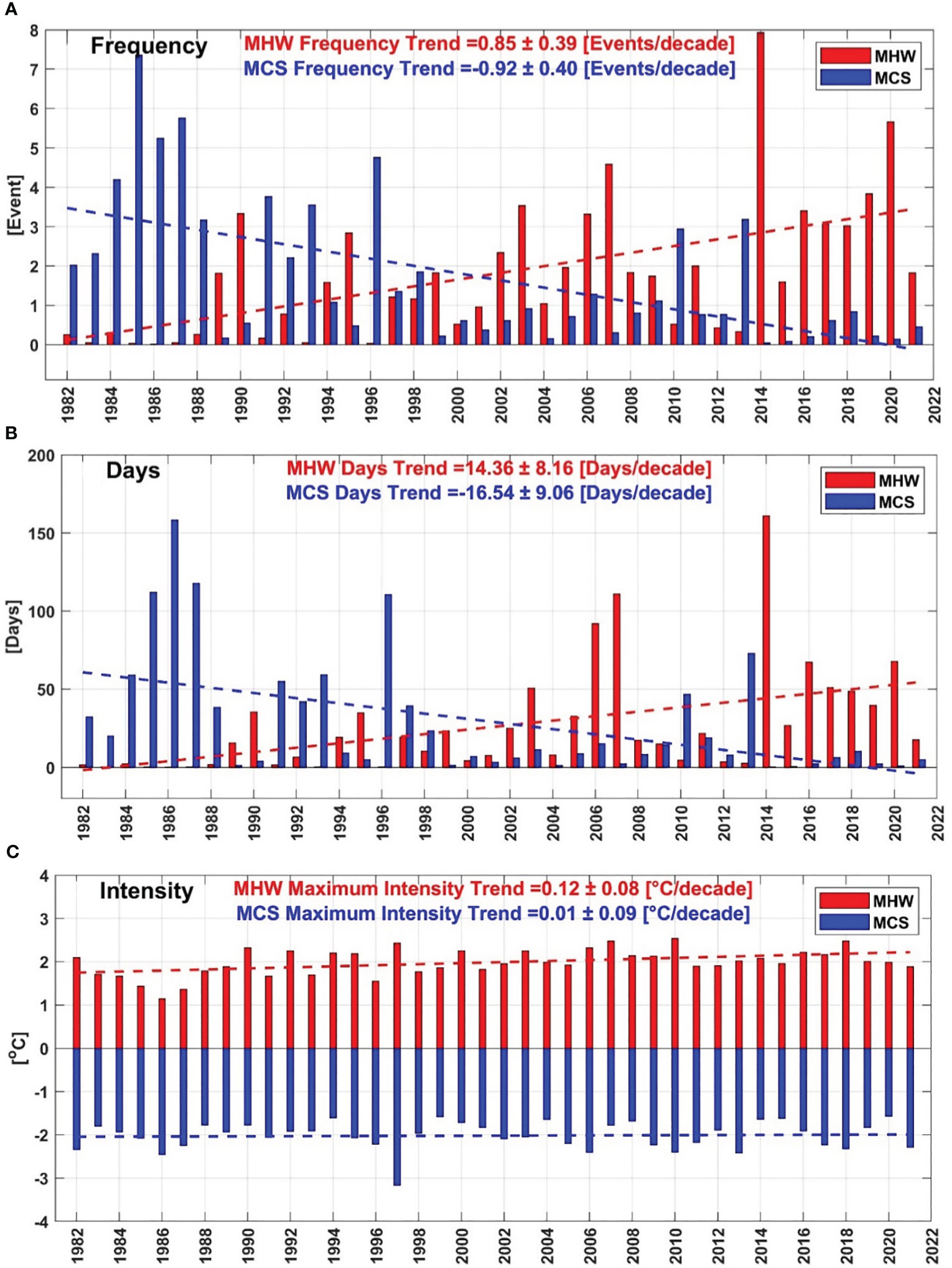
Figure 7 Regionally averaged annual mean MHW/MCS (A) frequency, (B) days, and (C) maximum intensity from 1982 to 2021. The red and blue bars represent MHW and MCS, respectively. The red and blue dashed lines represent the best-fit linear curves of the MHW and MCS characteristics, respectively. Note that the trend values are also displayed at the top of each subgraph.
Figure 7 shows the annual evolution of the frequency, total number of days, and maximum intensity of MHW (red bars) and MCS (blue bars) observed at all grid points over the southern North Sea throughout the study period. The highest annual MHW frequency was observed in 2014 (8 events, with a total of 160 MHW days), followed by 2020 (5 events, with 68 MHW days), and 2007 (4 events, with 110 MHW days) (see Figures 7A, B, red bars). The highest MCS frequency was recorded in 1985 (7 events, with 112 MCS days), followed by 1986 (5 events, with 158 MCS days), 1987 (5 events, with 117 MCS days), and 1996 (4 events, with 110 MCS days) (see Figures 7A, B, blue bars). These results are consistent with the SSTA (see Figure 3), where the highest MHW and MCS frequency occurred in the warmest and coldest years, respectively.
MHW and MCS characteristics (frequency, days, and maximum intensity) over the southern North Sea show a clear temporal trend from 1982 to 2021 (red and blue dashed lines in Figures 7A–C). Statistically significant (p < 0.05) increasing trends in annual MHW frequency and MHW days are observed over the study period (1982-2021), with trends of 0.85 ± 0.39 events/decade and 14.36 ± 8.16 days/decade, respectively (Figures 7A, B). The trend in MCS frequency and MCS days is of similar magnitude but decreases by about -0.92 ± 0.39 events/decade and -16.54 ± 9.06 days/decade, respectively (Figures 7A, B). The trend of maximum MHW intensity is 0.12 ± 0.08°C/decade, which is higher than the trend of maximum MCS intensity of 0.01 ± 0.09°C/decade (Figure 7C). Note that the MCS intensity is a negative value (blue bars in Figure 7C), and therefore, a positive trend in the maximum MCS intensity over time implies a weakening of the MCS.
On the decadal scale, the total number of MHWs increases from one decade to the next, whereas MCS have become less frequent since 1982 (Table 1; Figure 8). Figure 8 shows the annual MHW and MCS frequency versus their maximum intensities. The mean annual MHW frequency is increasing, especially in the last decade (2012–2021) with a record of 31 MHW events in this decade, 8 events in winter and 10 events in summer (Table 1), accounting for about 43%, 50% and 43% of the total annual, winter and summer events, respectively. Only five years (2004, 2010, 2012, 2013, and 2015) in the last two decades (2002-2021) have multiple MHWs below the climatological mean (1982-2021) annual MHW frequency (1.8 events, vertical dashed black line in Figure 8A), while only two years (1990 and 1995) in the first two decades (1982-2001) exceeded the mean annual MHW frequency. This increase in frequency is particularly notable in the last 10 years, as 2011, 2013, and 2015 are the only years below the mean value. Regarding the maximum intensity of MHW, there is neither a clear trend nor a clear relationship between the maximum intensity of MHW and the frequency. However, it can be observed that the MHWs have become more intense in most years of the last two decades, with the MHW maximum intensity above the annual average (1.98°C, horizontal dashed blue line in Figure 8A). The total number of MHW days has also gradually increased in the southern North Sea over the last two decades, especially in the last decade (red circles).
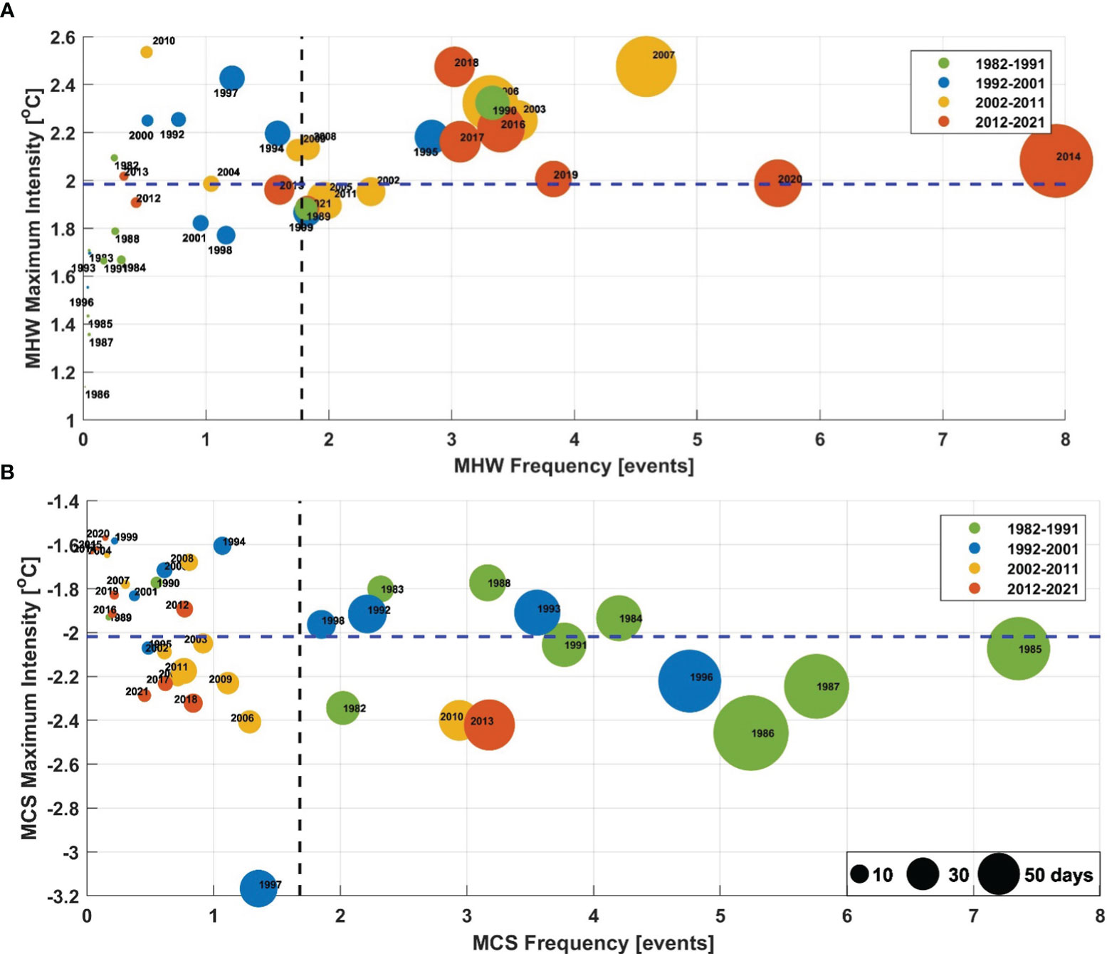
Figure 8 Annual mean maximum intensity versus frequency and total number of days in the southern North Sea by decade. (A) MHW, and (B) MCS. The dashed lines indicate the mean values for maximum intensity (horizontal) and frequency (vertical). The size of the colored circles indicates the annual average of total days. The black circles in the southeast corner of (B) represent the reference size of the circle for 10, 30, and 50 days.
The lowest MCS frequency was observed in the last two decades, especially in the last decade (2012-2021), where only 7 MCS events occurred, 5 events in winter and 2 events in summer (Table 1), representing about 10%, 14%, and 6% of the total annual winter and summer events, respectively. More than half of all MCSs detected during the analysis period occurred in the first decade (see Table 1). Only two years (2010 and 2013) in the last two decades (2002-2021) have a higher MCS frequency than the climatological mean (1982-2021) of annual MCS frequency (1.7 events, vertical dashed black line in Figure 8B). In the last decade, MCS are less intense and shorter (red circles) than in the first decade (green circles). In general, a large increase in MHW frequency and total days were observed in the last two decades, while MCSs generally decreased.
To explore the effects of large-scale teleconnection patterns (e.g., AMO, NAO, and EAP) on the annual variations of MHW and MCS in the southern North Sea, we first examine the relationship between annual SST and these climate indices (Figures 9A–C). We then examine the relationship between these climate indices with MHW/MCS frequency and total days at the annual and seasonal scales (Figures 9D–I, Table 2). We note that on the annual scale, both the AMO and EAP have a highly significant correlation (p < 0.05) with SST over the entire southern North Sea (Figures 9A, B), while the NAO is not statistically significantly (p > 0.05) correlated with SST (Figure 9C). The highest correlation between SST and AMO is found in the regions directly influenced by the inflow of warm Atlantic water (i.e., the northwestern part of the study area and the English Channel), as shown in Figure 9A. The highest correlation between SST and EAP is observed over the same region that has a stronger SST trend (i.e., the SST trend and the correlation between SST variability and EAP show similar patterns) (see Figures 4. 9B). This result indicates that the increase in surface air temperature seems to drive the SST trends in the southern North Sea, since the positive phases of the EAP are always associated with above-average surface air temperatures in Europe throughout the year.

Figure 9 Spatial distribution of correlation coefficients (R) between annual SST (top panels), MHW frequency (middle panels), and MCS frequency (bottom panels) with the different climate modes (A, D, G) AMO, (B, E, H) EAP, and (C, F, I) NAO from 1982 to 2021. Dotted areas indicate that the correlations are not statistically significant at the 95% confidence level (p > 0.05).
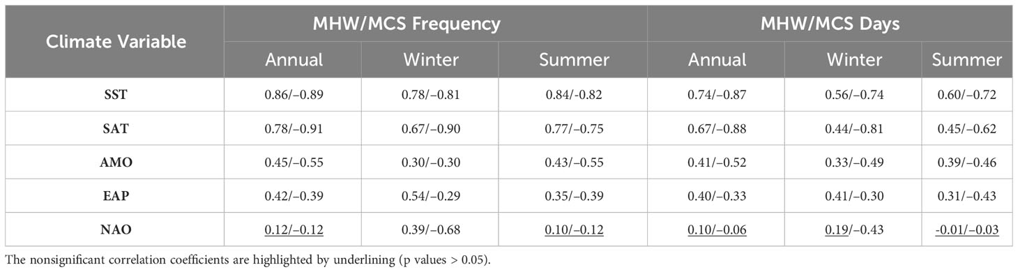
Table 2 Correlation coefficients (R) between MHW/MCS frequency and total days with climate modes (AMO, EAP, and NAO) and variables (SST and SAT) between 1982 and 2021.
We also found that at the annual scale, the frequency of MHW (MCS) had a statistically significant (p < 0.05) positive (negative) correlation with both AMO and EAP indices over most of the southern North Sea (Figures 9D, E, G, H). A non-significant correlation between the MHW frequencies and EAP was found only in the deep-water regions (e.g., in the northern of English Channel and south of the Dogger Bank, see Figure 9E), while the highest correlation with the AMO is found in the northwestern part of the southern North Sea (Figure 9D). In addition, the EAP and AMO indices have a significant positive (negative) correlation with MHW (MCS) total days (Table 2). There is no significant correlation between the NAO and the frequency or total days of MHW and MCS at the annual scale (Figures 9F, I, Table 2). Generally, on the seasonal and annual scale, significant correlations were found between the frequency and total days of MHW and MCS with two climate indices (AMO and EAP, see Table 2). This suggests that the MHW and MCS variations in the southern North Sea can be attributed to the AMO and atmospheric changes driven by the EAP climate modes. In contrast, NAO correlated only with the frequency of MHW (R= 0.39) and MCS (R= -0.68) and MCS days (R= -0.43) in winter (Table 2), whereas NAO did not correlate significantly with either the frequency of MHW and MCS or MHW and MCS days in summer (Table 2).
Furthermore, both SST and SAT showed highly significant correlation with MHW/MCS characteristics (frequency and total days). The positive correlation of MHW frequency with SAT (R= 0.78) is similar in strength to the correlation with SST (R= 0.86), and the same is true for MHW days, but shows a lower correlation with SAT (0.67) and SST (R=0.74). MCS frequency shows a strong negative correlation with SST (R= - 0.86) and SAT (R= - 0.91), and a higher negative correlation was also found between MCS days with SST (R=-0.87) and SAT (R=-0.88). This indicates that both oceanic and atmospheric warming play an important role in the formation of MHW in the southern North Sea. The relationship between MHW characteristics, SST, and SAT is stronger in summer than in winter, while the reverse was found for MCS characteristics (Table 2).
To better understand the distinct effects of the different phases of AMO, EAP, and NAO on the MHW or MCS in the southern North Sea, we performed a composite analysis by calculating the average frequency of MHW or MCS associated with the positive (> 1 standard deviation) and negative (< -1 standard deviation) phases of each climate mode (Figures 10, S3–S5). In this way, we obtain a clearer representation of the constructive and destructive influences associated with each phase. Compared to the negative phases of these climate modes, the annual frequency of MHW increased significantly in the positive phases (Figure S3). During the positive phases of AMO, EAP, and NAO, the average annual MHW frequency was found to be 2.53, 2.94, and 1.6 events, respectively. In contrast, considering only the negative phases of AMO, EAP, and NAO, the average annual frequency of MHW was 0.47, 0.80, and 0.74 events, respectively (Figure S3). The largest difference in MHW frequency between the positive and negative phases of the AMO index is found in the region affected by warm Atlantic water (i.e., the northwestern part of the southern North Sea, see Figure S3C). The atmospheric climate modes (i.e., EAP and NAO) control the westerly winds in the North Atlantic. The positive phases of these climate indices are associated with strong westerly winds leading to increased inflow of Atlantic water into the North Sea (van der Molen and Pätsch, 2022), while the negative phases represent weak westerly winds (Becker and Pauly, 1996).
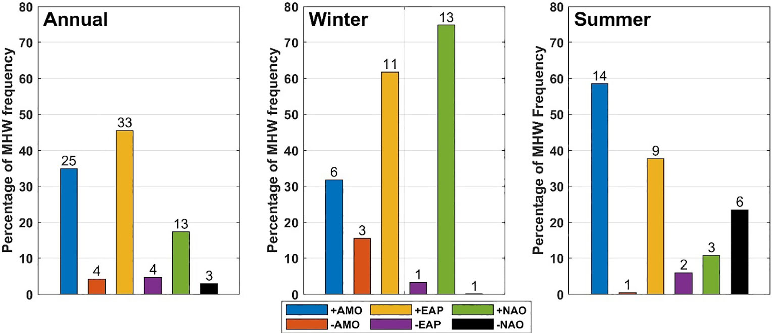
Figure 10 The percentage of MHW events coinciding with different phases (positive and negative) of three selected climate modes (AMO, EAP, and NAO) on the annual and seasonal scales. The total number of MHW events in each phase is shown above the bars.
In addition, Figure 10 shows the percentage of occurrence of MHW with different phases of the three selected climate modes (AMO, EAP and NAO). On the annual scale, both AMO and EAP influence SST (Figures 9A, B). However, the EAP has the strongest influence on the occurrence of MHW (Figure 10). Particularly, when the EAP is in a positive phase, the probability of MHW occurrence increases. More than 45% (33 MHW events out of 71 events) of MHW occurred during the positive EAP phase, whereas only 4 MHW events (5%) occurred during the negative EAP phase. For the AMO index, 35% of MHW (25 MHW events out of 71 events) occurred in the positive AMO phase, while only 4 MHW events occurred in the negative AMO phase. On the seasonal scale, the coexistence rate of MHWs with positive AMO modes is higher in summer than in winter, and the opposite was found for the EAP. Although the NAO does not correlate with MHW frequency at the annual scale (Table 2), more than 70% of the observed winter MHWs occurred during the positive phase of the NAO. The strong correlation and stronger coexistence of MHWs with the EAP and AMO modes indicate that the EAP and AMO modes play an important role in modulating MHWs in the North Sea. From the composite MCS analysis (Figures S4, S5), the negative phase of the AMO index had the strongest influence on the occurrence of MCS. On the annual scale, approximately 39% of MCS events (26 MCS events out of 67 events) occurred during the negative AMO phase (i.e., mainly before 1998, see Figure S2C). On the seasonal scale, the coexistence rate of MCSs with negative AMO modes is higher in summer (57%) than in winter (30%). In general, this composite analysis strengthens our previous correlation results (Figure 9) and confirms that MHW frequency is higher during the positive phases of these climate modes than during their negative phases. For MCS, the opposite is true.
Here, we explore the MHW and MCS events that occurred between 2013 and 2014 and the role of atmospheric conditions in the development of one of these events as a case study. As shown in Section 3.3, the highest MHW frequency was recorded in 2014 (8 events, with a total of 160 MHW days), while the highest MCS frequency in the last two decades was recorded in 2013 (3 events with a total of 73 MCS days). All these MHWs and MCSs were classified as moderate events because the SSTAs were above/below the difference between the 90th/10th percentile and the climatological mean (Hobday et al., 2018). The duration of these events reached 50 days for MHWs and 38 days for MCSs. The longest and most intense MCS event occurred in spring, while the longest but not the most intense MHW occurred in Autumn (Figure 11).
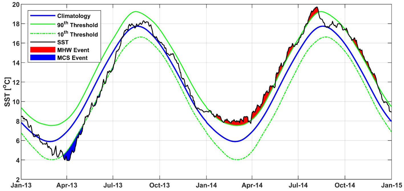
Figure 11 Daily time series of SST (in black) of the averaged southern North Sea between 2013 and 2014. The blue, green, and green dashed lines indicate the climatological mean, 90th, and 10th percentiles, respectively. The red and blue areas above and below the black curve indicate the MHW and MCS, respectively.
The case study considered here as spring MCS, which covered more than 90% of the study area, lasted from March 25 to May 1, 2013 (hereafter MCS13) and spring MHW, which covered 79% of the study area, lasted from March 31 to May 9, 2014 (hereafter MHW14), see Figure 11. MCS13 was the most intense in terms of SSTA (-2.14°C), mean intensity (-2.1°C), maximum intensity (-3.5°C), with an average absolute SST of 5.3°C. It was also the longest MCS in the last two decades, with a duration of 38 days. MHW14 had an average SSTA (1.62°C), mean intensity (1.12°C), maximum intensity (2.67°C), and an average absolute SST of about 9.1°C. The SSTAs and atmospheric conditions in April 2013 and April 2014 of MCS13 and MHW14 are shown in Figures 12A–F. During MCS13, pronounced cold (i.e., negative SSTA) was observed over the entire southern North Sea, with the highest negative anomalies (up to -3°C) along the Dutch and Belgian shelves (Figure 12A), while during MHW14, pronounced warmth (i.e., positive SSTA) was also observed over the entire southern North Sea (Figure 12B), with the highest values (up to 3°C) mainly in the same regions that exhibited negative anomalies during MCS13.
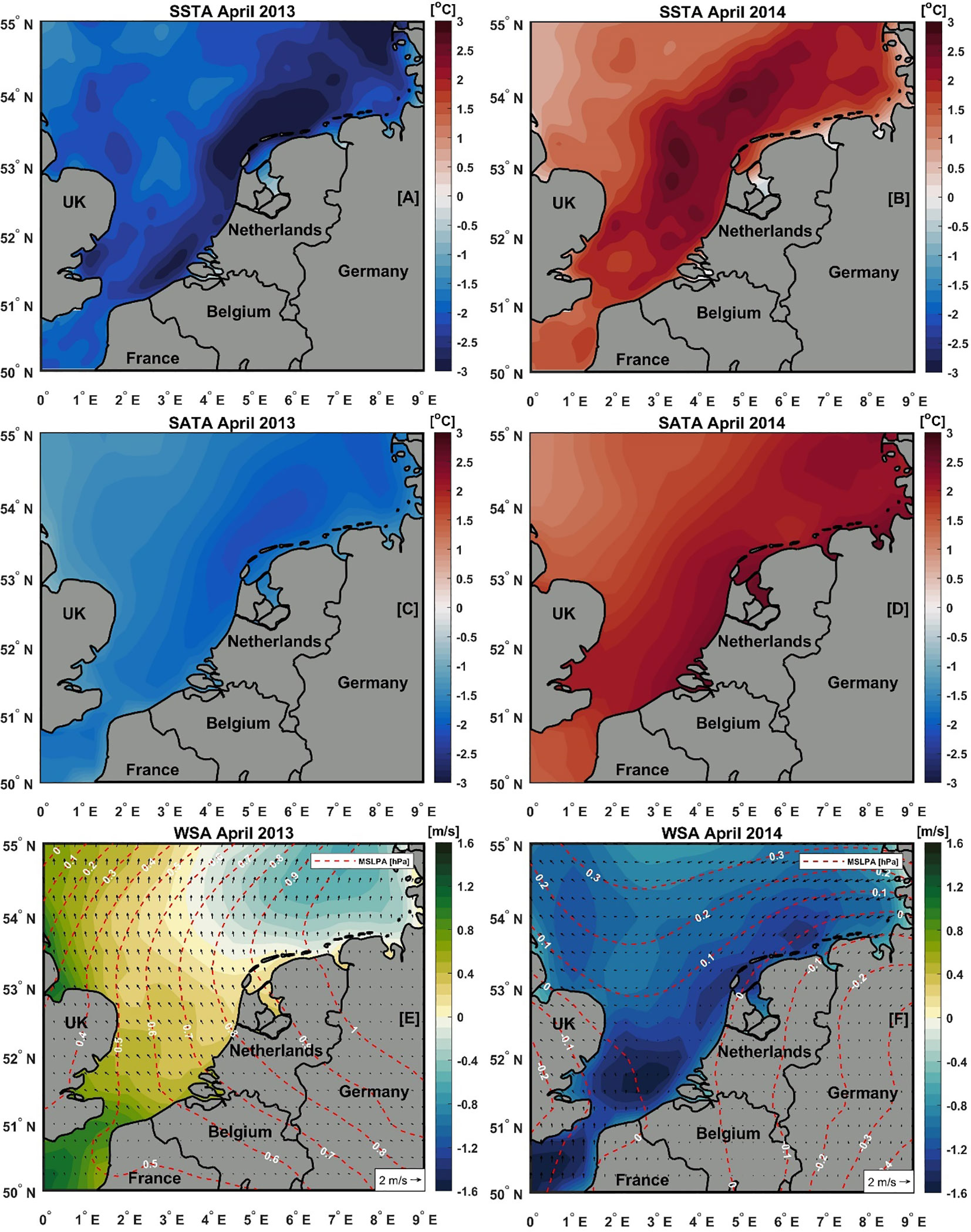
Figure 12 Composite map of anomalies in SST and atmospheric conditions during the April 2013 MCS (left) and April 2014 MHW (right) in the southern North Sea. (A, B) Sea surface temperature anomaly (SSTA, °C). (C, D) Surface air temperature anomaly (SATA, °C). (E, F) Wind speed anomalies (WSA, unit: m/s, vectors are wind direction; the shaded is magnitude). The dashed red lines show the mean sea level pressure anomaly (MSLPA, hPa).
The strong significant correlation between MHW/MCS and atmospheric factors suggests that atmospheric factors are the most important driver of MHW/MCS in the southern North Sea. In addition, previous studies in the North Sea (Becker and Pauly, 1996; Tinker and Howes, 2020), have concluded that atmospheric influences play a larger role in SST variability than oceanic influences. Therefore, the atmospheric forcings were analyzed here to explore their role in the generation of these extreme events. Atmospheric conditions during MCS13 (April 2013) showed overcooling of surface air temperature across the study region (Figure 12C), with the highest negative SAT anomalies in the same region that had the greatest negative intensity of this MCS event (Figure S6A). During the cold event (MCS13), SLP anomalies over the study region showed a zonally increasing gradient from west to east (red contour lines, Figure 12E), with an increase in absolute (Figure S7E) and anomalous wind speed values (shading, Figure 12E), showing an anticyclonic anomaly with southeasterly winds over the regions that had higher negative SSTA. The strong wind speed, especially the offshore winds (Figure 12E), could increase the vertical instability of the water column and increase the vertical mixing that brings cold water from the lower layer to the surface and cools the upper layer (Chen et al., 2022) increasing the possibility of MCS occurrence. Moreover, this MCS was associated with a strong negative phase NAO (Figure S2A).
During the warm event (MHW14), SLP anomalies showed a positive value over the ocean and a negative value over the land (red contour lines, Figure 12F). This resulted in a warm air temperature over the southern North Sea (Figure 12D) and a decrease in surface winds (Figure 12D). Averaged positive SAT anomalies reached 1.6°C in April 2014, which was one of the warmest years in recent decades (Figure S8B). The largest decrease in absolute values (Figure S7F) and anomalies (Figure 12F) of wind speed was observed in the English Channel and along the Belgian and Dutch shelves. As shown in Figure 12F, wind speed decreases by 1 m/s in most of the southern North Sea. The reduction in wind speed could enhance the thermal stratification of the water column and prevent the warm SST from mixing with the cold water below the surface, contributing to further warming of the surface water and thus the occurrence of the MHWs. This result indicates that the 2014 MHW is likely due to atmospheric forcing. However, with the anomalous SST warming, there was also an anomalous southeasterly wind over the English Channel, which could enhance the influx of warm Atlantic water into the North Sea. Therefore, further data sets and analysis are needed to investigate the local dynamic factors responsible for the development of MHW in the North Sea, including the role of oceanic forcing (e.g., heat advection by ocean currents) in the trend and variability identified in this study.
In this study, we quantified and compared the mean values and trends of MHW and MCS in the southern North Sea over the last four decades (1982-2021). We then described their seasonal and interannual evolution, as well as their possible relationship with large-scale climate modes (e.g., AMO, NAO, and EAP). The main conclusions of this study are summarized below.
The long-term warming SST trend in the southern North Sea showed a regional variation between 0.1 and 0.5°C/decade. The lowest SST trends were observed in coastal areas (e.g., along the northern Dutch coast and in the German Bight), while the highest SST trends were observed in the central and northeastern parts of the southern North Sea. This could be due to the accumulation of warm Atlantic water in these regions. The overall SST trend was about 0.33 ± 0.06°C/decade between 1982 and 2021. High spatial variability was also observed in mean MHW and MCS total days and maximum intensity. Regions with high MHW and MCS maximum intensity coincide with regions with high SST variability (see Figures 2D, 5B, D). The long-term warming trend of SST in the southern North Sea also increased the frequency and total number of MHW days to 0.85 ± 0.39 events/decade and 14.36 ± 8.16 days/decade, respectively. In contrast, the frequency and total number of MCS days showed the opposite trend, reaching -0.92 ± 0.39 events/decade and -16.54 ± 9.06 days/decade, respectively. There were no significant trends in the maximum intensity of MHW and MCS.
The composite analysis of MHW frequency with different phases of AMO, EAP, and NAO (Figures 10, S3, Table 2) showed the role of AMO and EAP in regulating MHW in the southern North Sea at the annual scale and NAO in winter. At the annual and seasonal scales, we found that positive AMO and EAP phases considerably increase the probability of MHW occurrence in the southern North Sea, while the NAO was the largest contributor only in winter. On an annual basis, we found that about 45%, 33%, and 18% of the total observed MHWs (71 events) occurred during positive EAP, AMO, and NAO phases, respectively. During winter, more than 70% of the MHW events occurred when the NAO index was in positive phase. The highest annual mean MHW frequency was associated with the positive phases of EAP (2.94 events), AMO (2.53 events), and NAO (1.6 events), while it was lower during the negative phases of these climate modes. This result suggests that the positive phases of these climate modes may be a favorable condition for a more frequent occurrence of MHW in the southern North Sea. This was also confirmed by the correlation analysis between MHW frequency and these climate modes (Figure 9) and by comparing MHW statistics during the positive and negative phases of the different climate modes (Figures S3, S4).
The highest correlation between SST and climate modes was found for the EAP index over the entire southern North Sea (Figure 9B), suggesting that atmospheric forcing has the largest influence on SST, consistent with previous studies (Becker and Pauly, 1996; Tinker and Howes, 2020). However, advective transports from the North Atlantic also play a role and likely explain part of the observed SST changes (Winther and Johannessen, 2006), particularly at the entrances to the North Sea, as indicated by the correlation between SST and the AMO index (Figure 9A), which is an indicator of AW inflow to the North Sea. We also found that MHW generally had a higher (lower) annual frequency during the positive (negative) phases of the EAP and AMO modes, which also showed a high correlation with annual MHW frequency. These results suggest that the annual variability of MHW in the southern North Sea could be attributed to the EAP-related atmospheric forcing and AMO. Moreover, our study showed that anomalous atmospheric warming and wind play a more important role in the formation of MHWs.
Overall, this study has improved our understanding of MHW and MCS in the southern North Sea, including their characteristics and their seasonal and interannual variability driven by low-frequency climatic modes such as AMO, EAP, and NAO. Future research needs to focus in more detail on specific MHW events (e.g., MHW 2022) to better understand the physical mechanisms and causes of these events, particularly ocean dynamic factors, including advection by ocean currents. This may include in situ data that include time series of the entire water column, not just SST, to examine the vertical extent of MHW from the surface to the subsurface (i.e., bottom MHW) and to estimate the heat budget of the mixed layer during these events. The earlier study by (Smale et al., 2019) identified the North Sea as a region where a high proportion of species are at the edge of their thermal tolerance range and high levels of non-climatic human stressors and intensification of MHW have affected the ecosystem (Tinker and Howes, 2020). A recent study (Alvera-Azcárate et al., 2021) has found that the spring bloom happens now one month earlier than 23 years ago. The causes of this phenology shift are still elusive, and the trend changes in extreme temperature observed in this study might help explaining partially this phenomenon. Thus, more research is needed to not only better understand but also monitor the consequences of these increasing MHW events in a region. Especially in the coastal environment and nearshore areas where important commercial fishing activities occur.
The original contributions presented in the study are included in the article/Supplementary Material. Further inquiries can be directed to the corresponding author.
BM: Conceptualization, Data curation, Formal Analysis, Funding acquisition, Investigation, Methodology, Project administration, Resources, Software, Supervision, Validation, Visualization, Writing – original draft, Writing – review & editing. AB: Conceptualization, Data curation, Formal Analysis, Funding acquisition, Investigation, Methodology, Project administration, Resources, Software, Supervision, Validation, Visualization, Writing – review & editing. AA-A: Conceptualization, Data curation, Formal Analysis, Funding acquisition, Investigation, Methodology, Project administration, Resources, Software, Supervision, Validation, Visualization, Writing – review & editing.
This work was fully funded by the STEREO-IV (Support To Exploitation and Research in Earth Observation) program administered by BELSPO (Belgian Science Policy Office) through the North-Heat project (STEREO-IV BELSPO # project SR/00/404).
The authors would like to thank the organizations that provided the data used in this work, including the Copernicus Marine Environment Monitoring Service (CMEMS), the European Centre for Medium-Range Weather Forecasts (ECMWF), and the National Oceanic and Atmospheric Administration (NOAA). We would also like to express our gratitude to the reviewers for their contributions to the development of this manuscript.
The authors declare that the research was conducted in the absence of any commercial or financial relationships that could be construed as a potential conflict of interest.
All claims expressed in this article are solely those of the authors and do not necessarily represent those of their affiliated organizations, or those of the publisher, the editors and the reviewers. Any product that may be evaluated in this article, or claim that may be made by its manufacturer, is not guaranteed or endorsed by the publisher.
The Supplementary Material for this article can be found online at: https://www.frontiersin.org/articles/10.3389/fmars.2023.1258117/full#supplementary-material
Aboelkhair H., Mohamed B., Morsy M., Nagy H. (2023). Co-occurrence of atmospheric and oceanic heatwaves in the eastern mediterranean over the last four decades. Remote Sens 5, 1841. doi: 10.3390/RS15071841
Alvera-Azcárate A., van der Zande D., Barth A., Troupin C., Martin S., Beckers J. M. (2021). Analysis of 23 years of daily cloud-free chlorophyll and suspended particulate matter in the greater north sea. Front. Mar. Sci. 8. doi: 10.3389/FMARS.2021.707632/BIBTEX
Becker G. A., Pauly M. (1996). Sea surface temperature changes in the North Sea and their causes. ICES J. Mar. Sci. 53, 887–898. doi: 10.1006/JMSC.1996.0111
Bond N. A., Cronin M. F., Freeland H., Mantua N. (2015). Causes and impacts of the 2014 warm anomaly in the NE Pacific. Geophys. Res. Lett. 42, 3414–3420. doi: 10.1002/2015GL063306
Borges A. V., Royer C., Martin J. L., Champenois W., Gypens N. (2019). Response of marine methane dissolved concentrations and emissions in the Southern North Sea to the European 2018 heatwave. Cont. Shelf Res. 190, 104004. doi: 10.1016/J.CSR.2019.104004
Chen K., Gawarkiewicz G., Kwon Y.-O., Zhang W. G. (2015). The role of atmospheric forcing versus ocean advection during the extreme warming of the Northeast U.S. continental shelf in 2012. J. Geophys. Res. Ocean. 120, 4324–4339. doi: 10.1002/2014JC010547
Chen K., Gawarkiewicz G. G., Lentz S. J., Bane J. M. (2014). Diagnosing the warming of the Northeastern U.S. Coastal Ocean in 2012: A linkage between the atmospheric jet stream variability and ocean response. J. Geophys. Res. Ocean. 119, 218–227. doi: 10.1002/2013JC009393
Chen W., Staneva J., Grayek S., Schulz-Stellenfleth J., Greinert J. (2022). The role of heat wave events in the occurrence and persistence of thermal stratification in the southern North Sea. Nat. Hazards Earth Syst. Sci. 22, 1683–1698. doi: 10.5194/NHESS-22-1683-2022
Ducrotoy J. P., Elliott M., De Jonge V. N. (2000). The north sea. Mar. pollut. Bull. 41, 5–23. doi: 10.1016/S0025-326X(00)00099-0
Frölicher T. L., Fischer E. M., Gruber N. (2018). Marine heatwaves under global warming. Nat 560, 360–364. doi: 10.1038/s41586-018-0383-9
Frölicher T. L., Laufkötter C. (2018). Emerging risks from marine heat waves. Nat. Commun. 9, 1–4. doi: 10.1038/s41467-018-03163-6
Garrabou J., Coma R., Bensoussan N., Bally M., Chevaldonné P., Cigliano M., et al. (2009). Mass mortality in Northwestern Mediterranean rocky benthic communities: effects of the 2003 heat wave. Glob. Change Biol. 15, 1090–1103. doi: 10.1111/J.1365-2486.2008.01823.X
Good S., Fiedler E., Mao C., Martin M. J., Maycock A., Reid R., et al. (2020). The current configuration of the OSTIA system for operational production of foundation sea surface temperature and ice concentration analyses. Remote Sens. 12. doi: 10.3390/rs12040720
Guiet J., Galbraith E., Kroodsma D., Worm B. (2019). Seasonal variability in global industrial fishing effort. PloS One 14. doi: 10.1371/JOURNAL.PONE.0216819
Hamdeno M., Alvera-Azcaráte A. (2023). Marine heatwaves characteristics in the Mediterranean Sea: Case study the 2019 heatwave events. Front. Mar. Sci. 10. doi: 10.3389/FMARS.2023.1093760/BIBTEX
Hamdeno M., Nagy H., Ibrahim O., Mohamed B. (2022). Responses of satellite chlorophyll-a to the extreme sea surface temperatures over the arabian and Omani gulf. Remote Sens. 14, 4653. doi: 10.3390/RS14184653
Hamed K. H., Ramachandra Rao A. (1998). A modified Mann-Kendall trend test for autocorrelated data. J. Hydrol. 204, 182–196. doi: 10.1016/S0022-1694(97)00125-X
Hersbach H., Bell B., Berrisford P., Hirahara S., Horányi A., Muñoz-Sabater J., et al. (2020). The ERA5 global reanalysis. Q. J. R. Meteorol. Soc 146, 1999–2049. doi: 10.1002/qj.3803
Hobday A. J., Alexander L. V., Perkins S. E., Smale D. A., Straub S. C., Oliver E. C. J., et al. (2016). A hierarchical approach to defining marine heatwaves. Prog. Oceanogr. 141, 227–238. doi: 10.1016/j.pocean.2015.12.014
Hobday A. J., Oliver E. C. J., Gupta A., Benthuysen J. A., Burrows M. T., Donat M. G., et al. (2018). Categorizing and naming marine heatwaves. Oceanography 31, 162–173. doi: 10.5670/oceanog.2018.205
Hobday A. J., Pecl G. T. (2014). Identification of global marine hotspots: Sentinels for change and vanguards for adaptation action. Rev. Fish Biol. Fish. 24, 415–425. doi: 10.1007/S11160-013-9326-6/FIGURES/3
Holbrook N. J., Scannell H. A., Sen Gupta A., Benthuysen J. A., Feng M., Oliver E. C. J., et al. (2019). A global assessment of marine heatwaves and their drivers. Nat. Commun. 10, 1–13. doi: 10.1038/s41467-019-10206-z
Holbrook N. J., Sen Gupta A., Oliver E. C. J., Hobday A. J., Benthuysen J. A., Scannell H. A., et al. (2020). Keeping pace with marine heatwaves. Nat. Rev. Earth Environ. 1, 482–493. doi: 10.1038/s43017-020-0068-4
Hurrell J. W., Kushnir Y., Ottersen G., Visbeck M. (2003). An overview of the north atlantic oscillation. Geophys. Monogr. Ser. 134, 1–35. doi: 10.1029/134GM01
IPCC (2021)Summary for policymakers. In: Climate change 2021: The physical science basis. Contribution of working group I to the sixth assessment report of the intergovernmental panel on c (Cambridge Univ. Press). Available at: https://www.ipcc.ch/report/ar6/wg1/chapter/summary-for-policymakers/ (Accessed May 25, 2023).
Kirby R. R., Beaugrand G., Lindley J. A., Richardson A. J., Edwards M., Reid P. C. (2007). Climate effects and benthic–pelagic coupling in the North Sea. Mar. Ecol. Prog. Ser. 330, 31–38. doi: 10.3354/MEPS330031
Knight J. R., Allan R. J., Folland C. K., Vellinga M., Mann M. E. (2005). A signature of persistent natural thermohaline circulation cycles in observed climate. Geophys. Res. Lett. 32, 1–4. doi: 10.1029/2005GL024233
Kueh M.-T., Lin C.-Y. (2020). The 2018 summer heatwaves over northwestern Europe and its extended-range prediction. Sci. Rep. 10, 1–18. doi: 10.1038/s41598-020-76181-4
Mills K. E., Pershing A. J., Brown C. J., Chen Y., Chiang F. S., Holland D. S., et al. (2013). Fisheries management in a changing climate: Lessons from the 2012 ocean heat wave in the Northwest Atlantic. Oceanography 26. doi: 10.5670/OCEANOG.2013.27
Mohamed B., Nilsen F., Skogseth R. (2022a). Interannual and decadal variability of sea surface temperature and sea ice concentration in the barents sea. Remote Sens. 14, 4413. doi: 10.3390/RS14174413
Mohamed B., Nilsen F., Skogseth R. (2022b). Marine heatwaves characteristics in the barents sea based on high resolution satellite data, (1982–2020). Front. Mar. Sci. 9. doi: 10.3389/FMARS.2022.821646
Oliver E. C. J. (2019). Mean warming not variability drives marine heatwave trends. Clim. Dyn. 53, 1653–1659. doi: 10.1007/S00382-019-04707-2
Oliver E. C. J., Benthuysen J. A., Bindoff N. L., Hobday A. J., Holbrook N. J., Mundy C. N., et al. (2017). The unprecedented 2015/16 Tasman Sea marine heatwave. Nat. Commun. 8, 1–12. doi: 10.1038/ncomms16101
Oliver E. C. J., Burrows M. T., Donat M. G., Sen Gupta A., Alexander L. V., Perkins-Kirkpatrick S. E., et al. (2019). Projected marine heatwaves in the 21st century and the potential for ecological impact. Front. Mar. Sci. 6. doi: 10.3389/FMARS.2019.00734/BIBTEX
Oliver E. C. J. J., Donat M. G., Burrows M. T., Moore P. J., Smale D. A., Alexander L. V., et al. (2018). Longer and more frequent marine heatwaves over the past century. Nat. Commun. 9, 1–12. doi: 10.1038/s41467-018-03732-9
Pastor F., Khodayar S. (2023). Marine heat waves: Characterizing a major climate impact in the Mediterranean. Sci. Total Environ. 861, 160621. doi: 10.1016/J.SCITOTENV.2022.160621
Roberts S. D., Van Ruth P. D., Wilkinson C., Bastianello S. S., Bansemer M. S. (2019). Marine heatwave, harmful algae blooms and an extensive fish kill event during 2013 in south Australia. Front. Mar. Sci. 6. doi: 10.3389/fmars.2019.00610
Sandler D., Harnik N. (2020). Future wintertime meridional wind trends through the lens of subseasonal teleconnections. Weather Clim. Dyn. 1, 427–443. doi: 10.5194/WCD-1-427-2020
Scannell H. A., Pershing A. J., Alexander M. A., Thomas A. C., Mills K. E. (2016). Frequency of marine heatwaves in the North Atlantic and North Pacific since 1950. Geophys. Res. Lett. 43, 2069–2076. doi: 10.1002/2015GL067308
Schlegel R. W., Darmaraki S., Benthuysen J. A., Filbee-Dexter K., Oliver E. C. J. (2021a). Marine cold-spells. Prog. Oceanogr. 198, 102684. doi: 10.1016/J.POCEAN.2021.102684
Schlegel R. W., Oliver E. C. J., Chen K. (2021b). Drivers of marine heatwaves in the northwest atlantic: the role of air–sea interaction during onset and decline. Front. Mar. Sci. 8. doi: 10.3389/FMARS.2021.627970/BIBTEX
Schlegel R. W., Oliver E. C. J., Wernberg T., Smit A. J. (2017). Nearshore and offshore co-occurrence of marine heatwaves and cold-spells. Prog. Oceanogr. 151, 189–205. doi: 10.1016/J.POCEAN.2017.01.004
Schlegel R., Smit A. (2018). heatwaveR: A central algorithm for the detection of heatwaves and cold-spells. J. Open Source Software 3, 821. doi: 10.21105/JOSS.00821/STATUS.SVG
Selig E. R., Casey K. S., Bruno J. F. (2010). New insights into global patterns of ocean temperature anomalies: Implications for coral reef health and management. Glob. Ecol. Biogeogr. 19, 397–411. doi: 10.1111/J.1466-8238.2009.00522.X
Sen Gupta A., Thomsen M., Benthuysen J. A., Hobday A. J., Oliver E., Alexander L. V., et al. (2020). Drivers and impacts of the most extreme marine heatwaves events. Sci. Rep. 10, 19359. doi: 10.1038/s41598-020-75445-3
Smale D. A., Wernberg T., Oliver E. C. J., Thomsen M., Harvey B. P., Straub S. C., et al. (2019). Marine heatwaves threaten global biodiversity and the provision of ecosystem services. Nat. Clim. Change 9, 306–312. doi: 10.1038/s41558-019-0412-1
Smith K. E., Burrows M. T., Hobday A. J., King N. G., Moore P. J., Sen Gupta A., et al. (2023). Biological impacts of marine heatwaves. Ann. Rev. Mar. Sci. 15, 119–145. doi: 10.1146/ANNUREV-MARINE-032122-121437
Smith K. E., Burrows M. T., Hobday A. J., Sen Gupta A., Moore P. J., Thomsen M., et al. (2021). Socioeconomic impacts of marine heatwaves: Global issues and opportunities. Sci. (80-.). 374. doi: 10.1126/science.abj3593
Tinker J., Howes E. L. (2020). The impacts of climate change on temperature (air and sea), relevant to the coastal and marine environment around the UK. MCCIP Science Review. doi: 10.14465/2020.arc01.tem
Trainer V. L., Kudela R. M., Hunter M. V., Adams N. G., McCabe R. M. (2020). Climate extreme seeds a new domoic acid hotspot on the US west coast. Front. Clim. 0. doi: 10.3389/FCLIM.2020.571836
Trenberth K. E., Shea D. J. (2006). Atlantic hurricanes and natural variability in 2005. Geophys. Res. Lett. 33, 12704. doi: 10.1029/2006GL026894
Tuckett C. A., Wernberg T. (2018). High latitude corals tolerate severe cold spell. Front. Mar. Sci. 5. doi: 10.3389/FMARS.2018.00014/BIBTEX
van der Molen J., Pätsch J. (2022). An overview of Atlantic forcing of the North Sea with focus on oceanography and biogeochemistry. J. Sea Res. 189, 102281. doi: 10.1016/J.SEARES.2022.102281
Wang Y., Kajtar J. B., Alexander L. V., Pilo G. S., Holbrook N. J. (2022). Understanding the changing nature of marine cold-spells. Geophys. Res. Lett. 49, e2021GL097002. doi: 10.1029/2021GL097002
Wang F., Shao W., Yu H., Kan G., He X., Zhang D., et al. (2020). Re-evaluation of the power of the mann-kendall test for detecting monotonic trends in hydrometeorological time series. Front. Earth Sci. 8. doi: 10.3389/feart.2020.00014
Wilks D. S. (2011). Statistical methods in the atmospheric sciences (Cambridge, MA: Academic Press).
Winther N. G., Johannessen J. A. (2006). North Sea circulation: Atlantic inflow and its destination. J. Geophys. Res. 111, 12018. doi: 10.1029/2005JC003310
Yao Y., Wang C. (2022). Marine heatwaves and cold-spells in global coral reef zones. Prog. Oceanogr. 209, 102920. doi: 10.1016/J.POCEAN.2022.102920
Yao Y., Wang C., Fu Y. (2022). Global marine heatwaves and cold-spells in present climate to future projections. Earth’s Futur. 10, e2022EF002787. doi: 10.1029/2022EF002787
Keywords: marine heatwaves, marine cold-spells, Southern North Sea, ERA5, Atlantic multidecadal oscillation, climate change
Citation: Mohamed B, Barth A and Alvera-Azcárate A (2023) Extreme marine heatwaves and cold-spells events in the Southern North Sea: classifications, patterns, and trends. Front. Mar. Sci. 10:1258117. doi: 10.3389/fmars.2023.1258117
Received: 13 July 2023; Accepted: 05 September 2023;
Published: 19 September 2023.
Edited by:
Kyung-Ae Park, Seoul National University, Republic of KoreaReviewed by:
You-Soon Chang, Kongju National University, Republic of KoreaCopyright © 2023 Mohamed, Barth and Alvera-Azcárate. This is an open-access article distributed under the terms of the Creative Commons Attribution License (CC BY). The use, distribution or reproduction in other forums is permitted, provided the original author(s) and the copyright owner(s) are credited and that the original publication in this journal is cited, in accordance with accepted academic practice. No use, distribution or reproduction is permitted which does not comply with these terms.
*Correspondence: Bayoumy Mohamed, YmEubW9oYW1lZEB1bGllZ2UuYmU=; bS5iYXlvdW15QGFsZXh1LmVkdS5lZw==
Disclaimer: All claims expressed in this article are solely those of the authors and do not necessarily represent those of their affiliated organizations, or those of the publisher, the editors and the reviewers. Any product that may be evaluated in this article or claim that may be made by its manufacturer is not guaranteed or endorsed by the publisher.
Research integrity at Frontiers
Learn more about the work of our research integrity team to safeguard the quality of each article we publish.