Foraging movements of humpback whales relate to the lateral and vertical distribution of capelin in the Barents Sea

Understanding how individual animals modulate their behaviour and movement patterns in response to environmental variability plays a central role in behavioural ecology. Marine mammal tracking studies typically use physical environmental characteristics that vary, and/or proxies of prey distribution, to explain predator movements. Studies linking predator movements and the actual distributions of prey are rare. Here we analysed satellite tag data from ten humpback whales in the Barents Sea (north-east Atlantic) to examine how their spatial movement and dive patterns are influenced by the geographic and vertical distribution of capelin, which is a key prey species for humpback whales. We used capelin density estimates based on direct observations from a trawl-acoustic survey and sun elevation to explore the drivers of changes in movement patterns. We found that the humpback whales’ exhibited characteristic area restricted search movement where capelin density was the highest. While horizontal movements showed both positive and negative individual relationships with sun elevation, humpback whale dive depth was positively correlated with diurnal variations in the vertical distribution of capelin. This suggests that in addition to whales foraging in regions of high capelin density, they also target the densest shoals of capelin at a range of depths, throughout the day and night. Overall, our findings suggest that regions of high capelin density are important foraging grounds for humpback whales, highlighting the central role capelin plays in the Barents Sea marine ecosystem.

1 Introduction

The distribution, availability, abundance, and type of prey strongly influences the behaviour of marine predators (Womble et al., 2014; Goldbogen et al., 2015; Hays et al., 2016). Marine predators may adapt both their horizontal and vertical movements in response to changes in patchy prey distribution to optimise their foraging efficiency3 (Boyd, 1996; Sims et al., 2008; Bestley et al., 2010; Thums et al., 2011; Bestley et al., 2015; Joy et al., 2015). Optimal foraging theory predicts that predators should concentrate their efforts on high prey density patches while minimising the transit time between prey patches to maximise their net energy gain and ultimately their fitness (Hedenström and Alerstam, 1997; Houston and McNamara, 2014). During foraging, marine predators commonly exhibit area-restricted search (ARS) behaviour, characterised by reduced speeds and increased turning rates to remain within a prey patch (Kareiva and Odell, 1987; Witteveen et al., 2008; Hazen et al., 2009; Jonsen et al., 2005; Breed et al., 2009; McClintock et al., 2012; Silva et al., 2013). In contrast, movement associated with transit displays consistent and elevated speeds with lower turning rates (Fauchald and Tveraa, 2003). When prey density declines in a particular area, predators may either leave in search of another high-density patch, or switch to alternate prey species (Murdoch, 1969; Van Baalen et al., 2001; Vogel et al., 2021). Therefore, movement analysis of predators can be linked to areas of high prey density.

The humpback whale (Megaptera novaeangliae) is a cosmopolitan species, with several distinct stocks identified around the world (Gulland, 1966; Stone et al., 1990; Baker et al., 1993; Rasmussen et al., 2007). Humpback whales typically migrate yearly between high latitude feeding areas and low latitude breeding grounds (Clapham, 2009). Their main feeding grounds are generally nutrient rich waters, where their diet consists of a variety of patchily distributed prey including fish, krill, copepods, and squid (Baker et al., 1985; Clapham and Palsbøll, 1997; Clapham, 2009; Meynecke et al., 2021).

The northeast Atlantic is regarded as a highly productive area, in particular the Barents Sea (Sakshaug and Slagstad, 1991; Sakshaug, 1997; Carmack and Wassmann, 2006). This area has some of the world’s largest pelagic fish stocks, such as Norwegian spring-spawning herring (Clupea harengus), capelin (Mallotus villosus) and cod (Gadus morhua). Northeast Arctic cod and haddock are the largest stocks of these species in the world (Hop and Gjøsæter, 2013; Hansen et al., 2019; Johannesen et al., 2019). The high productivity of this area also supports a large biomass of marine predators such as cetaceans, pinnipeds, seabirds and large fishes (Skern-Mauritzen et al., 2022). Marine predators are frequently observed in these productive waters exploiting the abundant prey resources (Gjøsæter et al., 2009; van der Meeren and Prozorkevich, 2019; Hamilton et al., 2021; Skern-Mauritzen et al., 2022). During the summer and autumn, northeast Atlantic humpback whales forage throughout the Norwegian and Barents Seas and around Iceland (Christensen et al., 1992; Leonard and Øien, 2020; Hamilton et al., 2021), and at least some proportion of the population also make use of abundant resources well into the winter season (Kettemer et al., 2022).

In the Barents Sea, humpback whales have been assumed to feed mainly on herring, capelin, and krill (Løviknes et al., 2021). In the last decades, an increase of humpback whales and other baleen whales in the northern Barents Sea has been attributed to growing fish stocks (Leonard and Øien, 2020). More generally, feeding hotspot areas in the Barents Sea for several marine mammal species overlap with the main feeding ground for adult capelin feeding on krill (van der Meeren and Prozorkevich, 2019; Hamilton et al., 2021). During summer months, shoals of capelin migrate to central and northern areas of the Barents Sea to feed, primarily on copepods and krill (Dalpadado et al., 2012; Dalpadado and Mowbray, 2013). While in these summer feeding grounds, capelin undertake diel vertical migrations, with a tendency to aggregate at deeper depths during the day and disperse towards the surface at night (Dalpadado and Mowbray, 2013; Skaret et al., 2020 Fall et al., 2021). This pattern is believed to be linked to variations in light intensity. The tendency of capelin to undertake vertical migrations is attributed to following their primary prey, krill, which utilise diel vertical migration to evade visual predators. Similarly, capelin themselves likely also migrate to avoid their visual predators (Gjøsæter, 1998; Hop and Gjøsæter, 2013).

Two feeding modes are generally observed for humpback whales: ram feeding and lunge feeding (Goldbogen et al., 2013). Ram feeding is characterised by whales swimming through dense prey schools at constant, slow speeds with their mouths open, forcing water through their exposed baleen plates (Goldbogen et al., 2013). Lunging, on the other hand, is characterised by whales engulfing a large volume of prey-filled water at high speed, thereafter, filtering the water out with their mouths closed (Goldbogen et al., 2013). Feeding can occur at the surface, in shallow waters, and/or at depth and at the bottom (Jurasz and Jurasz, 1979; Ware et al., 2011; Ware et al., 2014; Mastick et al., 2022). While little is known about how humpback whales locate and track prey patches, presumably they use multiple senses, such as visual, auditory, and olfactory. They may also use memory of previously visited areas, rely on cues from conspecifics or anthropogenic cues such as the presence of fishing vessels.

One common limitation of previous marine mammal predator-prey telemetry-based studies is that they use indirect proxies of prey distribution. In this study we are able to examine the links between predator movements and the distribution of a key prey resource, capelin. Moreover, we account for horizontal movements (c.f. Vogel et al., 2021), as well as for vertical movements of whales in relation to their prey. The main objective of this study is to assess the degree to which northeast Atlantic humpback whale diving behaviour and spatial distribution is influenced by the spatial and vertical distribution of capelin in the Barents Sea using satellite telemetry and large-scale acoustic survey data. Our study aims to investigate: (1) the association between Barents Sea capelin distribution and both horizontal and vertical movements of humpback whales, (2) whether diel variations in light levels influence the horizontal movement behaviour of humpback whales, (3) how diel variations in humpback whale diving correlates with capelin vertical distribution and (4) the presence of individual variation in the behavioural responses of whales to capelin density.

2 Materials and methods

2.1 Study site

Tagging (Figure 1A) was conducted between the 4^th and 9^th of September 2018 as part of a collaborative research cruise conducted between the University of Tromsø and Institute of Marine Research (IMR) within the Barents Sea, just east of Svalbard. The choice timing and location of tagging efforts was informed by previous humpback whale sightings data collected from prior annual Joint Norwegian/Russian ecosystem surveys in the Barents Sea and adjacent waters (van der Meeren and Prozorkevich, 2019). Tagging took place concurrently with the annual joint Barents Sea Norwegian/Russian ecosystem cruise (between August and October 2018) that was conducting its acoustic and biological surveying for capelin in the same area (dashed line, Figure 1A).

FIGURE 1

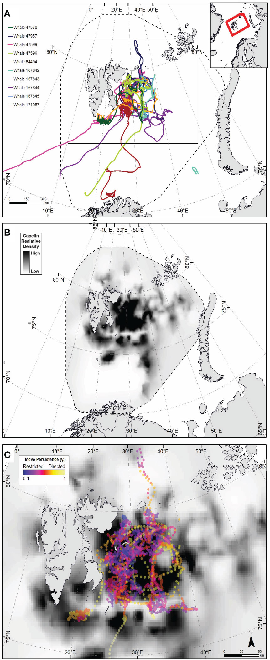
Figure 1 Tracks from 10 humpback whales (at 3-hr time interval steps) instrumented in the northern Barents Sea in September 2018 (A). Dashed line in (A, B) show the spatial extant of the capelin modelled density. Red Box in inset indicates the spatial frame of (A, B). (B) depicts the 2018 modelled relative capelin density distribution. Dark black indicates areas of higher relative density. (C) shows relative density of capelin with humpback whale move persistence (γ_t) estimate points between September 4^th 2018 and October 31st overlaid, where yellow points indicate high γ_t (i.e. transiting behaviour) and dark purples indicate low γ_t (i.e. restricted foraging behaviour).

2.2 Tagging methods

Ten subdermally-anchored satellite tags (5 SPOT-303 tags and 5 SPLASH-302 tags, Wildlife Computers, Redmond, WA) were deployed using an Aerial Rocket Tagging System (ARTS, Kleivane et al., 2022) following best tagging practices described by Andrews et al. (2019). Specifically, whales were slowly approached and tagged from a 20 ft open rigid inflatable boat. Tags were placed below the dorsal fin and were sterilised with 70% ethanol before deployment. When possible, photographs of the flukes were taken, enabling identification of the individual whales and ensuring that the same individual was not tagged twice. Tagging was approved by the Norwegian Food Safety Authority (Mattilsynet) under permit FOTS ID 14135 2017/279575.

The five deployed SPOT tags provided transmissions used to drive estimates of geographic position using the doppler-shift of the signals received by Argos satellite receivers, as described at https://www.argos-system.org. These tags were programmed to send ~15 transmissions per hour for the first four months, then reduce to 12 transmissions per hour for the following three months, before finally reducing to 80 transmission per day until their batteries failed or the tag was lost. This programming schedule allowed for high temporal resolution data early in the tagging period and then coarser data later to prolong battery life in cases when tags remained attached for longer periods than expected. The five SPLASH tags similarly transmitted horizontal position data, whilst additionally recording information on the diving behaviour of the tagged animal. These tags were programmed to transmit 400 data transmissions per day, in order to receive as much behavioural dive information as possible during the main period of interest, i.e. the summer feeding season.

2.3 Tag data processing

Tag location data were pre-processed by Argos-CLS using their Kalman filter (Lopez et al., 2014). All subsequent data processing and statistical analyses were carried out using the R programming language (version 4.2.2, R Core Team, 2022). A continuous-time correlated random walk state-space model (CRW) implemented in the ‘fit_ssm’ function in the ‘aniMove’ R package (Jonsen et al., 2023) was used to estimate the most probable paths taken by each whale (Jonsen et al., 2019; Jonsen et al., 2020; Jonsen et al., 2023). Specifically, the CRW represents the most likely path an animal took based on the pre-filtered ARGOS position estimates by converting the non-uniform time series to a regularised path (Johnson et al., 2008), accounting for location uncertainty and temporally-irregular transmissions (Jonsen et al., 2005). This model enabled us to estimate whale positions while accounting for location uncertainty at regularised 3-hour intervals. Substantial gaps in tracking data can present challenges when fitting these types of models, such as unreliable predictions during these periods of data absence. To mitigate this issue, whale tracks containing a gap greater than 1 week were split prior to CRW modelling and further statistical analysis. A split-track segment was included in subsequent analyses only if it had at least 20 consecutive raw data points and there was at least one position each day.

2.4 Humpback whale movements

2.4.1 Horizontal movements-move persistence (γ_t)

Move persistence (γ_t) is a behavioural index that considers autocorrelation between consecutive movements of animal track locations and accounts for changes across both speed and heading (Jonsen et al., 2019). This continuous metric ranges from 0, indicating highly tortuous movements typically within a restricted area, associated with e.g. searching or foraging, to 1, representing consistent movements in terms of both directionality and speed (Jonsen et al., 2019). We selected move persistence as our metric of humpback whale horizontal movement behaviour, because it provides a continuous scale that allows for subtle difference in movement behaviour, rather than defining somewhat arbitrary discrete behavioural states (Breed et al., 2012; Auger-Méthé et al., 2017; Eisaguirre et al., 2019; Jonsen et al., 2019). The ‘fit_mpm’ function in the ‘aniMotum’ R package (Jonsen et al., 2023) was used to estimate pooled move persistence from the location data.

2.4.2 Vertical movements

SPLASH tags were programmed to optimise data collection for behavioural dive data. The tags recorded maximum dive depth, dive duration, dive start- and end-time for dives that were ≥15 meters deep and ≥2 minutes in duration. Like the horizontal position data, this data was also transmitted using Argos satellite receivers.

2.5 Capelin density

Continuous acoustic data and biological data from trawl hauls were collected as part of the joint Russian/Norwegian annual Barents Sea ecosystem survey (Eriksen et al., 2018) between August and October 2018. The data were used to map the relative density of capelin in the Barents Sea where the 10 whales were tagged. Using a fleet of research vessels, the survey is designed to visit an equally-spaced station grid with 35 nautical miles between each station, where the ships collect trawl data, and other abiotic data. The vessels survey along transects connecting the stations, and additional transects between the station grid in the areas where most capelin is expected (van der Meeren and Prozorkevich, 2019). The vessels continuously sample acoustic echosounder data along the transects using SIMRAD EK60 or EK80 equipment calibrated according to standard procedures (Demer et al., 2015). The echosounder data were processed using the Large Scale Survey System software package as outlined by Korneliussen et al. (2006). The classification and allocation of acoustic backscattering to biological categories was done by experts on board using a combination of acoustic signal characteristics and pelagic trawl catches, and with ‘capelin’ as a target category. The resulting acoustic density values were stored by category as nautical area scattering coefficient (NASC; m²/nmi²) (Maclennan et al., 2002) with a horizontal resolution of 1 nautical mile and a vertical resolution of 10 m. The abundance estimate of capelin used for assessment purposes is made in StoX (Johnsen et al., 2019), and combines the acoustic data at the resolution of 1 nautical miles (Elementary Distance Sampling Unit; EDSU) with biological data within a given pre-defined stratum using transects as Primary Sampling Unit (PSU). We used the R-package ‘RstoX’ (Holmin, 2019; Johnsen et al., 2019) to link the per-stratum biological data to acoustic data to obtain capelin density as biomass per EDSU.

Based on the vertically integrated EDSU density estimates from the above analysis, we created an interpolated capelin density surface, using the Integrated Nested Approximation model (INLA) and Template Model Builder (TMB) frameworks as implemented in the ‘INLA’ and ‘sdmTMB’ packages (Rue et al., 2009; Lindgren et al., 2011; Martins et al., 2013; Lindgren and Rue, 2015; Kristensen et al., 2016; Anderson et al., 2022). Here, we used the INLA functionality to create irregular triangulated meshes covering the entire survey region, where the mesh size is adapted to the sampling resolution such that areas with denser number of data points are associated with smaller mesh sizes. We then developed a spatial interpolation model in TMB, where unexplained variation in density is assumed to follow a Gaussian Random Field (GRF) process, and where spatial autocorrelation is governed by a Matérn function with parameters estimated by TMB. To model spatial point processes, TMB uses the stochastic partial differential equation (SPDE) approach originally implemented in INLA (Rue et al., 2009; Lindgren and Rue, 2015). To account for the barrier effect caused by Svalbard’s coastline, supporting barrier models were employed, as described in Bakka et al. (2016, 2018, 2019). Together, these spatial point-process methods were used on the capelin density point values along transects to interpolate relative capelin density as described previously in Vogel et al. (2021). We assumed that the NASC-derived density values follow a negative binomial distribution. The resulting interpolated surface is thus assumed to represent the overall spatial capelin distribution throughout the entire the survey period (September – October), as well as the entire vertical water column. Hereafter we refer to the resulting interpolated density surface as the ‘relative capelin density field’.

2.6 Capelin density whale interactions

2.6.1 Horizontal interactions

To investigate how changes in time-varying move persistence (γ_t) calculated based on the whales’ three hrs-interpolated locations are influenced by environmental variables and how these relationships may vary between individuals, we used mixed-effect modelling using the ‘mpmm’ package in R (Auger-Méthé et al., 2017; Jonsen et al., 2019; Jonsen et al., 2020). Specifically, we examined two environmental variables potentially correlated with humpback whale horizontal movements: (1) horizontal capelin density and (2) sun angle (as a proxy for light intensity), which is thought to be correlated with vertical distribution of capelin (Gjøsæter, 1998; Mowbray, 2002). Light intensity was included to examine whether whales preferentially forage in lower light levels when capelin is closer to the surface, compared to when the capelin move down through the water column when light levels are higher. Based on the location and time of each whale track coordinate along each movement trajectory, a corresponding relative capelin biomass value was extracted from the relative capelin density field. Tracking points that occurred outside of this field were excluded from the analyses. Additionally, only tracking points that occurred in September or October 2018 were used in this study which overlapped with the capelin survey. Sun angle values were calculated for every point along each humpback whale trajectory based on their recorded location and time using the ‘solarpos’ function from the ‘maptools’ R package (Bivand and Lewin-Koh, 2021).

We modelled γ_t as a function of various combinations of the explanatory variables and random effects structures:

$$\text{logit}({\text{γ}}_{\text{t}})={\text{ρ}}_{\text{t}}+{\text{α}}_{\text{t}}+({\text{ρ}}_{\text{t}}+{\text{α}}_{\text{t}}| \text{id})$$

This equation allows for nine possible model permutations (Table 1) for how the two environmental explanatory variables (relative capelin density and sun angle) might influence whales move persistence. Fixed effects are represented by capelin density (ρ_t) and sun angle (α_t), and terms in parentheses indicate random slopes, with individual whale identifiers (id) representing random intercepts to assess the extent to which relationships may differ among individuals (see Jonsen et al., 2019 for further details). The models were ranked based on changes in Akaike’s information criterion (ΔAIC) and likelihood ratio (ΔLR).

TABLE 1

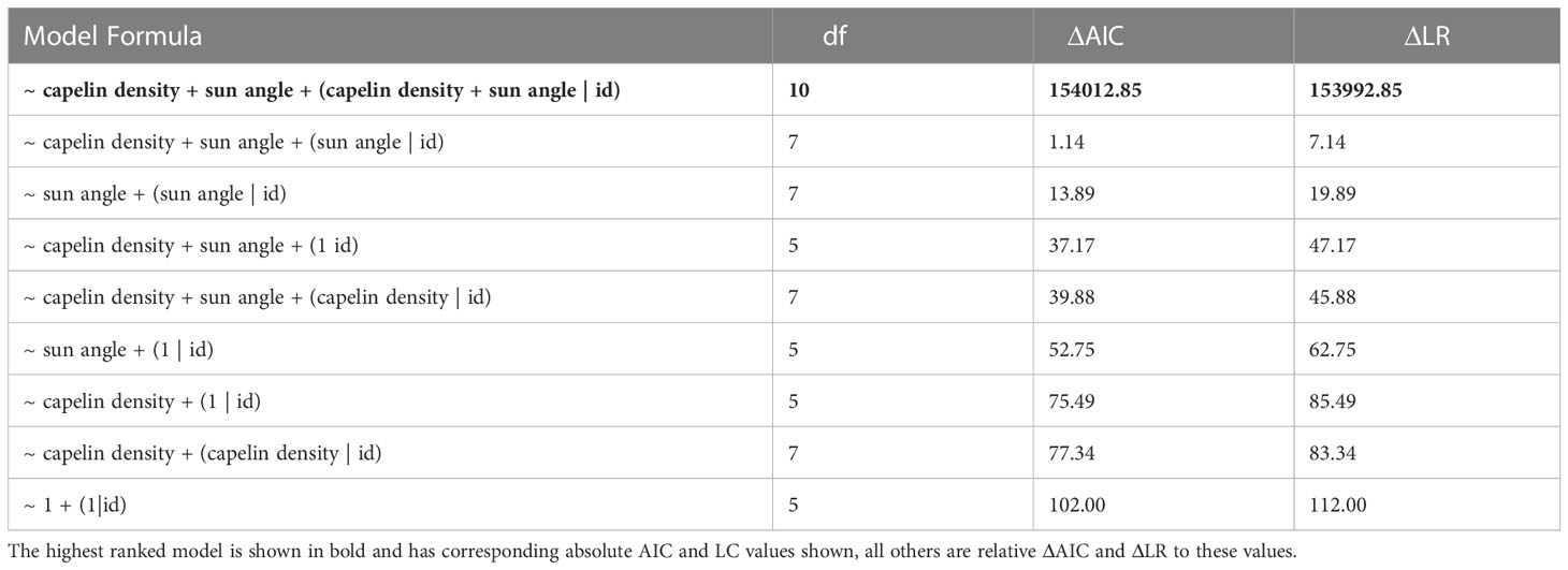
Table 1 Ranked list of mixed-effect models based on changes in Akaike’s information criterion (ΔAIC) and likelihood ratios (ΔLR).

2.6.2 Vertical interactions

To further investigate how humpback whale movements were influenced by the spatial characteristics of capelin, we also compared the five whales with dive data records (Table 2) to NASC-derived capelin density within the capelin acoustic survey area (Figure 1A, dashed line). Only dive data occurring between September 4^th 2018 (first day of tagging) and October 31^st 2018 were used for dive analysis. The calculated vertical capelin distribution (at 10-meter depth resolution) was derived from the acoustic NASC values collected from the capelin survey, regardless of geographic location within the survey area, and was segmented by time of day. To do this, we first calculated 25^th, 50^th and 75^th quantiles of humpback whale dive depths by hour using the ‘quantile’ function from the ‘qgam’ package (Fasiolo et al., 2017). We then calculated the mean NASC value of each 10m depth cell per hour. Using these depth bin averages, we calculated the weighted 25^th, 50^th and 75^th quantiles for the capelin data using the ‘Quantile’ function from the ‘DescTools’ package (Signorell, 2023). Since quantile capelin data are a function of the NASC measurements, the mean NASC values per cell were used to weight the capelin centre of mass values.

TABLE 2

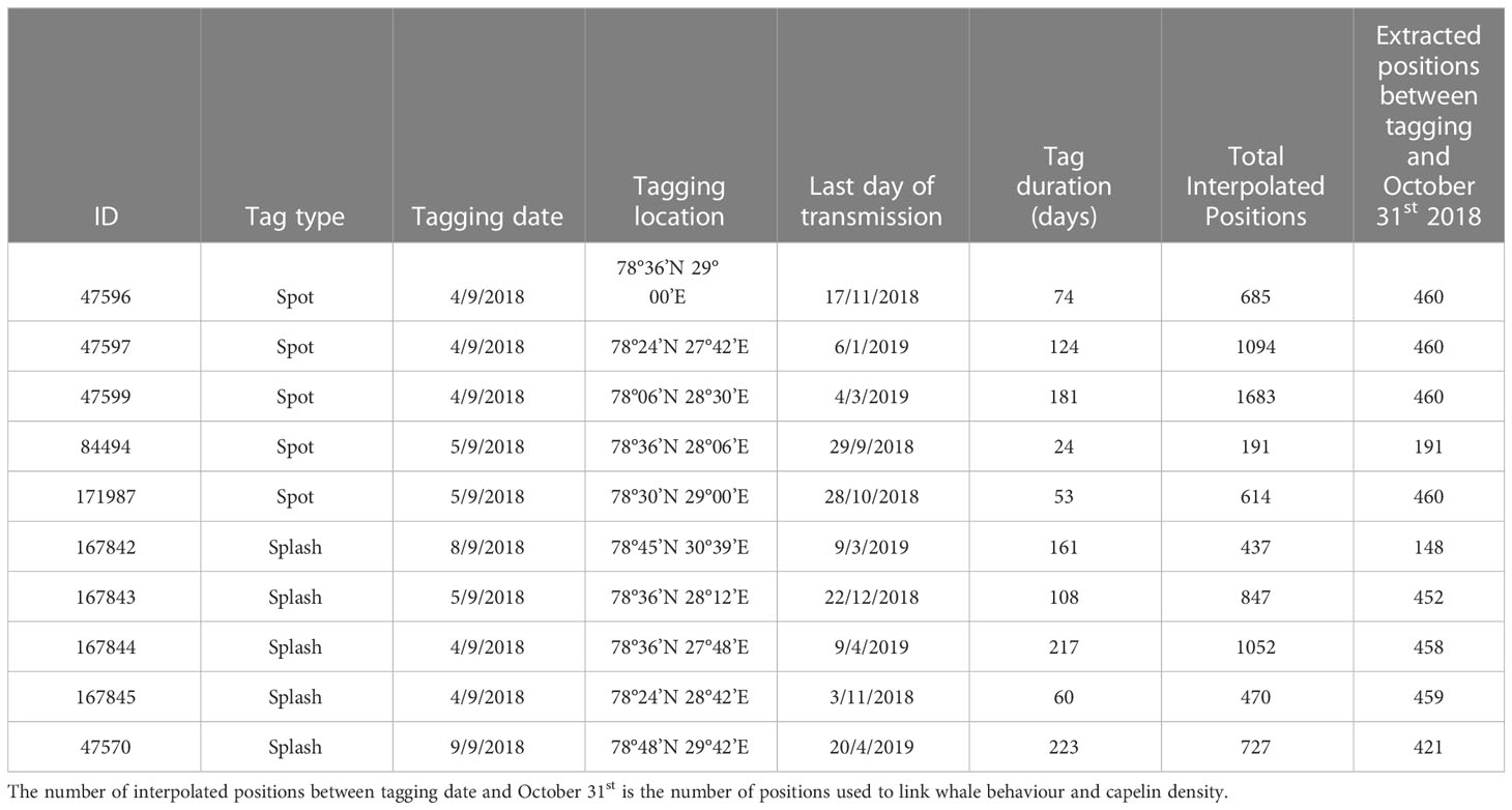
Table 2 Tag summary statistics.

To compare the whale dive depth with the weighted capelin depth, a Pearson’s product-moment correlation test was performed on the hourly 50% quantile (median) values of both datasets. A linear regression model was used with the ‘lm’ function from the ‘stats’ package (R Core Team, 2022), using the 50% quantile of the humpback whale dive depths by hour as the response variable and the weighted 50% quantile of capelin depth by hour as the predictor variable.

3 Results

3.1 Humpback whale tag performance

Tag duration was generally longer for Splash tags (60-223 days, mean=152, sd=55, n=5) than for Spot tags (24 –181 days, mean=92, sd=55, n=5) (Table 2). The period all ten whales were tracked within the area (Figure 1; Supplemental Figure 1) covered by the capelin surveys between tagging date and October 31^st ranged from 19 to 58 days (mean=50, sd=14). This gave a total of 208 whale-days of spatial overlap between capelin survey data and whale tracking data between tagging date and October 31^st that were used for subsequent capelin-humpback whale horizontal interaction analysis.

3.2 Horizontal humpback whale movements and distribution

The tracks of all ten whales exhibited highly clustered, tortuous movement patterns east of Svalbard on the Spitsbergen, Great and Central Banks (Figure 1A; Supplemental Figure 2), also reflected in clusters of low move persistence (Figure 1C), indicative of area-restricted search (ARS).

3.3 Vertical humpback behaviour

The Splash tags recorded 13,530 humpback whale dives in total (ranging from 120 for 5701 per individual), where 10,692 of the dives occurred during the capelin survey period (Table 3; Figure 2). Supplemental Figure 3 shows all recorded dives over a 5-month period for the 5 individuals tagged with Splash tags. A clear diurnal pattern can be seen is September and October (representing 79% of all dives recorded). A diurnal pattern was not observed in November, December, and January. Average dive depth across the full tracks of all individuals was 110 ± 80 meters, and average dive duration was 6 ± 3 minutes. Overall average dive depth between tagging and October 31^st and within the survey area was 110 ± 78 meters, and average dive duration was 5 ± 2 minutes. The maximum recorded dive depth for an individual whale between tagging and October 31^st was 352 meters.

TABLE 3

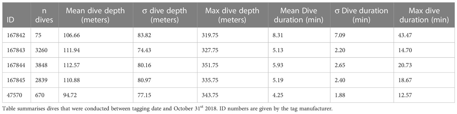
Table 3 Diving information from Splash satellite tags deployed on five individual humpback whales.

FIGURE 2

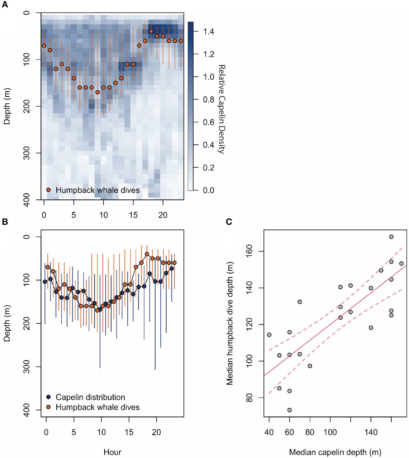
Figure 2 (A) shows relative capelin density throughout the water column and throughout the day from the IMR/PINRO Barents Sea Ecosystem Acoustic survey for capelin. The log transformed NASC values taken throughout the water column give a capelin density at 10 m depth bins. Here, dark blues indicate high relative capelin density and light blue indicate low relative capelin density. Superimposed over the capelin density is red points (representing median) and lines (representing 25-75% quantiles) of humpback dive depths. (B) again shows humpback whale dive depth median and 25%-75% quantiles in red with the same centre of mass capelin distribution in dark blue. Only dive data occurring between September 4^th 2018 (first day of tagging) and October 31^st 2018 were used because they overlapped temporally with the capelin survey. (C) shows the results from a linear regression model in red, with capelin median depth as the predictor and median humpback whale dive depth is the response variable.

The 50^th quantile of hourly humpback dive depths displays a clear diurnal pattern (Figure 2). On average, the whales dove deeper in the daytime between 06:00 and 13:00, and shallower at night between 16:00 and 00:00, with the intermediate hours spent shifting gradually.

3.4 Capelin-Humpback whale interactions

3.4.1 Horizontal interactions

There is a clear spatial co-occurrence between low move persistence areas of humpback whales and high capelin density patches (Figure 1D). On average, move persistence was inversely influenced by capelin biomass and sun angle (Table 3). The most parsimonious model, logit(γ_t) = ρ_t + α_t + (ρ_t + α_t | id), included random intercept and slope terms, suggesting that there are individual differences in overall movement characteristics between whales. On average, humpback whales tended to exhibit restricted movements in areas of high capelin densities, suggesting foraging behaviour (Figure 3A). All but two of the whales (ID 167845, and to a lesser degree, ID 167843, Supplemental Figure 4) responded this same way to changes in capelin biomass. The relationship between move persistence and sun angle was highly variable between individuals (Figure 3B), with seven individuals showing negative relationships while three had positive relationships. This suggests that humpback whales generally exhibit low move persistence when in high capelin density areas, whereas their relationship with sun angle is highly individual. The second ranked model logit (γ_t) = ρ_t + α_t + (α_t | id), was also considered based on its ΔAIC (<1.14) and its small LR values, as well as the belief that using AIC based rankings frequently selects for the most complex models (Wagenmakers and Farrell, 2004). This model considers capelin density as only influencing random intercepts, whilst sun angle was both random intercept and slope terms (Supplemental Figure 5). This model indicated that all whales responded this same way to changes in capelin density, however whales respond individually to changes in sun angle, suggesting no clear relationship at the population level.

FIGURE 3

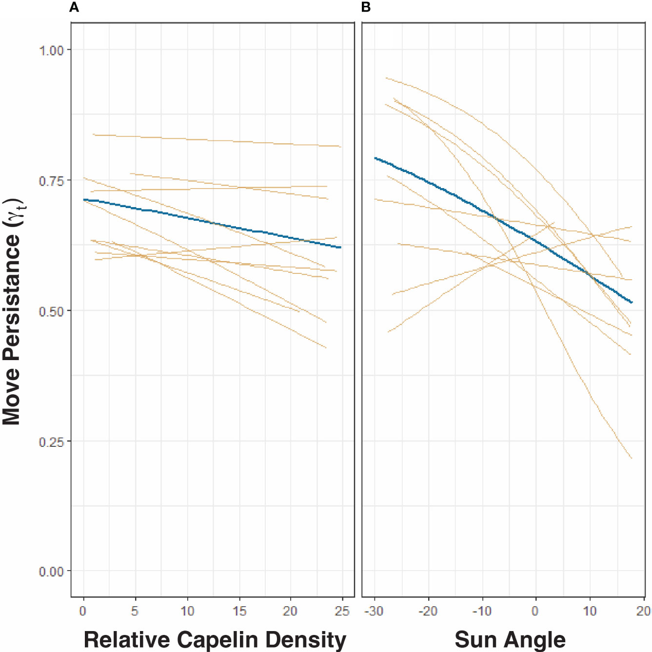
Figure 3 Most parsimonious model from mixed effect analysis of the relationship between humpback whale move persistence (γ_t) and relative capelin density (A) and sun angle (light intensity, (B). Fixed effects are depicted in blue and random effects in yellow. As per the most parsimonious model [logit(γ_t) = ρ_t + α_t + (ρ_t + α_tid)] in Table 2, both panels allow for random intercepts and random slopes.

3.4.2 Vertical interactions

We found a strong positive linear relationship between whale dive depth and capelin distribution (adjusted r² = 0.6086, p = 4.21e-06, Figure 2). This suggests that humpback whale dive depth increases with capelin depth.

4 Discussion

Humpback whales broadly follow the spatial distribution and vertical movements of capelin when on the summer feeding grounds in the Barents Sea. Reduced speed and directionality of horizontal movements within areas of high capelin density strongly suggest that humpback whales target high-density capelin areas. Past ecosystem surveys, opportunistic sightings, and whaling records have all indicated that the area east of the Svalbard archipelago is an important foraging ground for northeast Atlantic humpback whales during late summer and fall (Nøttestad et al., 2015; van der Meeren and Prozorkevich, 2018; Hamilton et al., 2021). In addition, Ressler et al. (2015) found, based on visual whale sightings and echosounder caplin data, that humpback whale distribution correlated with the acoustic estimates of capelin. Through the use of satellite tracking, our study expanded on Ressler et al. (2015) by correlating individual humpback whale movement behaviour with capelin density. This supports the hypothesis that capelin are either (A) directly a key prey species for humpback whales during the late summer in the Barents Sea, or (B) that capelin and humpbacks target the same prey species, such as copepods and krill. Regardless of whether either or both of these hypotheses are true, our finding of humpback whales foraging movements being influenced by changes in capelin density distribution supports the strong link between humpback whales and capelin.

In addition to the strong negative relationship between capelin biomass and move persistence, our most parsimonious model also suggested that light intensity influenced the movement behaviour of humpback whales. Overall, the negative relationship between light intensity and whale move persistence suggests that whales display area-restricted foraging behaviour at higher sun intensities. This could reflect the whales diving deeper during the day to reach the capelin that migrate to the deep when light intensities are stronger (Dalpadado and Mowbray, 2013; Skaret et al., 2020; Fall et al., 2021), and therefore the whales have restricted surface behaviours. However, the substantial variability in the individual responses to light intensity suggests that this relationship is not uniform across individuals and may simply be a spurious artifact. For example, this individual variability could be due to the variations across both tag retention time and the amount of time each whale spent within the geographical limits of the capelin surveys in the Barents Sea. Furthermore, seeing as in the summer, light is consistently intense (high sun angle) in the Barents Sea due to its high latitude. Some whales stayed in this northern foraging area throughout the polar night until as late as January, well after the sun has ceased to rise over the horizon. It is plausible that the 3 h reconstructed step intervals used in this study might not provide sufficient temporal resolution to detect variations in the horizontal whale movements caused by capelin diel vertical migrations (Postlethwaite and Dennis, 2013). Similarly, the vertical migrations of capelin in the water column only influence the dive depth patterns of humpback whales, and not their horizontal movements (or at least not at this resolution). This is consistent with our finding of whale depths consistently following the capelin depths throughout the day and night. This explanation agrees with recent pinniped studies that suggesting that both vertical and horizontal movements need to be considered when examining seal foraging (Bestley et al., 2015; Carter et al., 2016). Fine-scale studies of humpback whale diving behaviour in other regions (e.g. Friedlaender et al., 2013) have found strong diel variations in their dive behaviours relating to variations to their prey and its relationship to light.

We also showed a strong positive correlation between whale dive depth and vertical capelin distribution. During the capelin survey period, August-October, capelin were found concentrating at the surface at night and moving deeper during the day. Correspondingly, humpback whale dive depths (between September and October) also showed a diurnal vertical pattern matching the capelin distribution. This diel vertical pattern in humpback whale diving behaviour likely reflects feeding on the densest patches of capelin, suggesting that humpback whales adjust their diving behaviour in response to capelin density distributions in the water column. Our findings are consistent with previous studies showing that foraging humpback whales in other waters maximised their energetic gain by targeting the densest prey depth layers to optimise their energy efficiency (Goldbogen et al., 2008; Ware et al., 2011; Friedlaender et al., 2013; Burrows et al., 2016; Friedlaender et al., 2016). Our results also suggest that humpback whales may feed throughout the day and night, which may help explain the complex relationship between horizontal move persistence and sun angle. The diurnal pattern of whale dive depth observed in September and October was not observed in November, December, or January. This might be expected since the attenuation of diurnal diving patterns in other polar marine mammals has been observed in winter (Biuw et al., 2010). Furthermore, since the number of dives recorded in November, December and January were limited, and only represented 21% of the total dive data, it is possible that the limited number of dives was insufficient to statistically reveal any underlying dive depth patterns.

While our results suggest a strong correlation between capelin distribution and humpback whale movements, it should be noted that there are differences in the spatial and temporal coverage of these datasets that might inadvertently introduce bias. The capelin biomass density field is based on directly measured NASC-derived capelin density that was limited to the geographical range covered by the acoustic surveys. To accommodate this, we limited our analyses to use only humpback whale location points that fell within the survey region. Furthermore, since the annual Barents Sea ecosystem cruise that collected the capelin data used in this study was conducted between August and October 2018, our INLA analysis represents a static image of capelin density for this time-period. In contrast, our whale satellite tagging data sometimes extended for time periods past this period, and typically with higher temporal resolution. For this reason, the whale movement data used in our analysis, either horizontal or vertical, was truncated to only include data that matched both the geographic and temporal constraints of the capelin survey data. Our capelin density distribution models a static spatial distribution over the survey area, and our mixed-effects modelling assumes that this static distribution is representative of the capelin distribution over this time period. While the broad-scale spatial distribution of capelin is believed to remain relatively stable over the summer and fall months, we cannot discount the possibility of variations resulting from fine-scale physical and biological oceanic dynamics that might occur. These variations could potentially influence whale movements. Nonetheless, the fact that we observed correlations between our static capelin distribution and our dynamic whale horizontal movements suggest that our static image captures the key aspects of the capelin distribution during this period, and therefore provides valuable information about predator-prey interactions. Similar analyses have previously found good agreement between herring distribution and killer whale move movement patterns in the Norwegian Sea (Vogel et al., 2021).

Our comparison of whale depth movements and capelin depth distribution also involves certain assumptions related to the spatial and temporal distributions of capelin that again might inadvertently introduce bias. For this comparison, we aggregated all the capelin depth data, regardless of location, to create a matrix of capelin density as a function of depth over time. Similarly, our whale depth data was aggregated within the survey region, to reveal whale depth use as a function of time of the day. This analysis does not consider the possibility that the depth uses of capelin and whales might differ geographically over the survey area. Regardless, the strong correlation between whale and capelin hourly depth suggests that their depth uses were relatively stable across the survey region, and again provides insight into the humpback whale-capelin predator prey interactions. The vertical movements of diving air-breathing animals almost certainly influence their horizontal behaviour, and a horizontal movement model would therefore most likely be improved by inclusion of such vertical information (Bestley et al., 2015; McClintock et al., 2017). However, in this study, only half of the whales were tagged with Splash tags (n=5) that provided both horizontal and vertical movement information. While this limited sample size is likely be sufficient for providing an indication of the relationship between the vertical diving behaviour and the vertical prey distribution, these data were too sparse for developing and fitting a complex three-dimensional model. For this reason, we analysed the horizontal and vertical movement and prey distribution data separately. A comparative study of three-dimensional whale movement in relation to the three-dimensional distribution of their prey might add further insight into whale predator prey behaviour. Future studies using only Splash tags are warranted to explore this multidimensional analysis.

This study presents direct evidence of the influence capelin density has on humpback whale movements in the Barents Sea, without relying on prey proxies. It highlights the direct relationship between prey and predator movements, emphasizing the importance of measuring prey density for a deeper understanding of marine predator-prey dynamics. This study also provides a timepoint against which future changes in humpback whale foraging behaviour and responses to environmental changes can be assessed.

Data availability statement

The raw data supporting the conclusions of this article will be made available by the authors, without undue reservation.

Ethics statement

The animal study was approved by the Norwegian Food Safety Authority 123 (Mattilsynet) under permit FOTS ID 14135 2017/279575. The study was conducted in accordance with the local legislation and institutional requirements.

Author contributions

EV: Conceptualization, Data curation, Formal Analysis, Investigation, Methodology, Validation, Visualization, Writing – original draft, Writing – review & editing. SS: Data curation, Formal Analysis, Investigation, Writing – original draft. MB: Conceptualization, Investigation, Methodology, Supervision, Validation, Visualization, Writing – review & editing. M-AB: Formal Analysis, Investigation, Supervision, Writing – review & editing. LK: Data curation, Writing – review & editing. GS: Methodology, Validation, Writing – review & editing, Investigation. NØ: Data curation, Writing – review & editing. AR: Conceptualization, Funding acquisition, Investigation, Resources, Supervision, Writing – review & editing.

Acknowledgments

We thank the research teams and crew, in particular Kjell-Arne Fagerheim and Lisa Kettemer, for their support during fieldwork. This project was part of the “Whalefeast project” (financed by The Regional Research Council in Troms). We also thank Jennifer Arthur for her assistance in GIS to render the maps in our figures.

Conflict of interest

The authors declare that the research was conducted in the absence of any commercial or financial relationships that could be construed as a potential conflict of interest.

Publisher’s note

All claims expressed in this article are solely those of the authors and do not necessarily represent those of their affiliated organizations, or those of the publisher, the editors and the reviewers. Any product that may be evaluated in this article, or claim that may be made by its manufacturer, is not guaranteed or endorsed by the publisher.

Supplementary material

The Supplementary Material for this article can be found online at: https://www.frontiersin.org/articles/10.3389/fmars.2023.1254761/full#supplementary-material

References

Anderson S. C., Ward E. J., English P. A., Barnett L. A. K. (2022). sdmTMB: an R package for fast, flexible, and user-friendly generalized linear mixed effects models with spatial and spatiotemporal random fields. bioRxiv 2022.03.24.485545. doi: 10.1101/2022.03.24.485545

CrossRef Full Text | Google Scholar

Andrews R. D., Baird R. W., Calambokidis J., Goertz C. E., Gulland F. M., Heide-Jorgensen M. P., et al. (2019). Best practice guidelines for cetacean tagging. J. Cetacean Res. Manage. 20 (1), 27–66.

Google Scholar

Auger-Méthé M., Albertsen C. M., Jonsen I. D., Derocher A. E., Lidgard D. C., Studholme K. R., et al. (2017). Spatiotemporal modelling of marine movement data using Template Model Builder (TMB). Mar. Ecol. Prog. Ser. 565, 237–249. doi: 10.3354/meps12019

CrossRef Full Text | Google Scholar

Baker C. S., Herman L. M., Perry A., Lawton W. S., Straley J. M., Straley J. H. (1985). Population characteristics and migration of summer and late-season humpback whales (megaptera Novaeangliae) in Southeastern Alaska. Mar. Mammal Sci. 1 (4), 304–323. doi: 10.1111/j.1748-7692.1985.tb00018.x

CrossRef Full Text | Google Scholar

Baker C. S., Perry A., Bannister J. L., Weinrich M. T., Abernethy R. B., Calambokidis J., et al. (1993). Abundant mitochondrial DNA variation and world-wide population structure in humpback whales. Proc. Natl. Acad. Sci. U.S.A 90 (17), 8239–8243. doi: 10.1073/pnas.90.17.8239

PubMed Abstract | CrossRef Full Text | Google Scholar

Bakka H., Rue H., Fuglstad G. A., Riebler A. (2018). Spatial modeling with r-INLA: a review. Wiley Interdis- cip Rev. Comput. Stat. 10, e1443.

Google Scholar

Bakka H., Vanhatalo J., Illian J., Simpson D., Rue H. (2016). Accounting for physical barriers in species distribution modeling with non-stationary spatial random effects. arXiv:1608.03787.

Google Scholar

Bakka H., Vanhatalo J., Illian J. B., Simpson D., Rue H. (2019). Non-stationary gaussian models with physical barriers. Spat Stat. 29, 268–288.

Google Scholar

Bestley S., Jonsen I. D., Hindell M. A., Harcourt R. G., Gales N. J. (2015). Taking animal tracking to new depths: synthesiz- ing horizontal–vertical movement relationships for four marine predators. Ecology 96, 417–427. doi: 10.1890/14-0469.1

PubMed Abstract | CrossRef Full Text | Google Scholar

Bestley S., Patterson T. A., Hindell M. A., Gunn J. S. (2010). Predicting feeding success in a migratory predator: integrating telemetry, environment, and modeling techniques. Ecology 91 (8), 2373–2384.

PubMed Abstract | Google Scholar

Biuw M., Nøst O. A., Stien A., Zhou Q., Lydersen C., Kovacs K. M. (2010). Effects of hydrographic variability on the spatial, seasonal and diel diving patterns of southern elephant seals in the eastern Weddell Sea. PloS One 5 (11), e13816. doi: 10.1371/journal.pone.0013816

PubMed Abstract | CrossRef Full Text | Google Scholar

Bivand R., Lewin-Koh N. (2021). “maptools: Tools for Handling Spatial Objects,” in R package version 1, 1–2. Available at: https://CRAN.R-project.org/package=maptools.

Google Scholar

Breed G. A., Costa D. P., Jonsen I. D., Robinson P. W., Mills-Flemming J. (2012). State-space methods for more completely capturing behavioral dynamics from animal tracks. Ecol. Model. 235–236, 49–58. doi: 10.1016/j.ecolmodel.2012.03.021

CrossRef Full Text | Google Scholar

Boyd I. L. (1996). Temporal scales of foraging in a marine predator. Ecology 77 (2), 426–434.

Google Scholar

Breed G. A., Jonsen I. D., Myers R. A., Bowen W. D., Leonard M. L. (2009). Sex-specific, seasonal foraging tactics of adult grey seals (Halichoerus grypus) revealed by state–space analysis. Ecology 90, 3209–3221.

PubMed Abstract | Google Scholar

Burrows J. A., Johnston D. W., Straley J. M., Chenoweth E. M., Ware C., Curtice C., et al. (2016). Prey density and depth affect the fine-scale foraging behavior of humpback whales megaptera novaeangliae in sitka sound, alaska, USA. Mar. Ecol. Prog. Ser. 561, 245–260.

Google Scholar

Carmack E., Wassmann P. (2006). Food webs and physical–biological coupling on pan-Arctic shelves: Unifying concepts and comprehensive perspectives. Prog. Oceanography 71 (2), 446–477. doi: 10.1016/j.pocean.2006.10.004

CrossRef Full Text | Google Scholar

Carter M. I. D., Bennett K. A., Embling C. B., Hosegood P. J., Russell D. J. (2016). Navigating uncertain waters: a critical review of inferring foraging behaviour from location and dive data in pinnipeds. Mov Ecol. 4, 25. doi: 10.1186/s40462-016-0090-9

PubMed Abstract | CrossRef Full Text | Google Scholar

Christensen I., Haug T., Øien N. (1992). Seasonal distribution, exploitation and present abundance of stocks of large baleen whales (Mysticeti) and sperm whales (Physeter macrocephalus) in norwegian and adjacent waters. ICES J. Mar. Sci. 49 (3), 341–355.

Google Scholar

Clapham P. J. (2009). “Humpback Whale: Megaptera novaeangliae,” in Encyclopedia of Marine Mammals, 2nd ed. Eds. Perrin W. F., Würsig B., Thewissen J. G. M. (London: Academic Press), 582–585. doi: 10.1016/B978-0-12-373553-9.00135-8

CrossRef Full Text | Google Scholar

Clapham P. J., Palsbøll P. J. (1997). Molecular analysis of paternity shows promiscuous mating in female humpback whales (Megaptera novaeangliae, Borowski). Proc. R. Soc. London. Ser. B: Biol. Sci. 264 (1378), 95–98. doi: 10.1098/rspb.1997.0014

CrossRef Full Text | Google Scholar

Dalpadado P., Ingvaldsen R. B., Stige L. C., Bogstad B., Knutsen T., Ottersen G., et al. (2012). Climate effects on the Barents Sea ecosystem dynamics. ICES J. Mar. Sci. 69, 1303–1316. doi: 10.1093/icesjms/fss063

CrossRef Full Text | Google Scholar

Dalpadado P., Mowbray F. (2013). Comparative analysis of feeding ecology of capelin from two shelf ecosystems, off Newfoundland and in the Barents Sea. Prog. Oceanography 114, 97–105. doi: 10.1016/j.pocean.2013.05.007

CrossRef Full Text | Google Scholar

Demer D. A., Berger L., Bernasconi M., Bethke E., Boswell K., Chu D., et al. (2015). Calibration of acoustic instruments.

Google Scholar

Eisaguirre J. M., Auger-Méthé M., Barger C. P., Lewis S. B., Booms T. L., Breed G. A. (2019). Dynamic-parameter move- ment models reveal drivers of migratory pace in a soar- ing bird. Front. Ecol. Evol. 7, 317.

Google Scholar

Eriksen E., Gjøsæter H., Prozorkevich D., Shamray E., Dolgov A., Skern-Mauritzen M., et al. (2018). From single species surveys towards monitoring of the Barents Sea ecosystem. Prog. Oceanography 166, 4–14. doi: 10.1016/j.pocean.2017.09.007

CrossRef Full Text | Google Scholar

Fall J., Johannesen E., Englund G., Johansen G. O., Fiksen Ø. (2021). Predator–prey overlap in three dimensions: cod benefit from capelin coming near the seafloor. Ecography 44 (5), 802–815. doi: 10.1111/ecog.05473

CrossRef Full Text | Google Scholar

Fasiolo M., Goude Y., Nedellec R., Wood S. N. (2017) Fast calibrated additive quantile regression. Available at: https://arxiv.org/abs/1707.03307.

Google Scholar

Fauchald P., Tveraa T. (2003). Using first-passage time in the analysis of area-restricted search and habitat selection. Ecology 84, 282–288.

Google Scholar

Friedlaender A. S., Johnston D. W., Tyson R. B., Kaltenberg A., Goldbogen J. A., Stimpert A. K., et al. (2016). Multiple-stage decisions in a marine central-place forager. R. Soc. Open Sci. 3 (5), 160043. doi: 10.1098/rsos.160043

PubMed Abstract | CrossRef Full Text | Google Scholar

Friedlaender A. S., Tyson R. B., Stimpert A. K., Read A. J., Nowacek D. P. (2013). Extreme diel variation in the feeding behavior of humpback whales along the western Antarctic Peninsula during autumn. Mar. Ecol. Prog. Ser. 494, 281–289. doi: 10.3354/meps10541

CrossRef Full Text | Google Scholar

Gjøsæter H. (1998). The population biology and exploitation of capelin (Mallotus villosus) in the Barents Sea. Sarsia 83 (6), 453–496. doi: 10.1080/00364827.1998.10420445

CrossRef Full Text | Google Scholar

Gjøsæter H., Bogstad B., Tjelmeland S. (2009). Ecosystem effects of the three capelin stock collapses in the Barents Sea. Mar. Biol. Res. 5 (1), 40–53. doi: 10.1080/17451000802454866

CrossRef Full Text | Google Scholar

Goldbogen J. A., Calambokidis J., Croll D. A., Harvey J. T., Newton K. M., Oleson E. M., et al. (2008). Foraging behavior of humpback whales: Kinematic and respiratory patterns suggest a high cost for a lunge. J. Exp. Biol. 211 (23), 3712–3719. doi: 10.1242/jeb.023366

PubMed Abstract | CrossRef Full Text | Google Scholar

Goldbogen J. A., Friedlaender A. S., Calambokidis J., McKenna M. F., Simon M., Nowacek D. P. (2013). Integrative approaches to the study of baleen whale diving behavior, feeding performance, and foraging ecology. Bioscience 63 (2), 90–100. doi: 10.1525/bio.2013.63.2.5

CrossRef Full Text | Google Scholar

Goldbogen J. A., Hazen E. L., Friedlaender A. S., Calambokidis J., DeRuiter S. L., Stimpert A. K., et al. (2015). Prey density and distribution drive the three-dimensional foraging strategies of the largest filter feeder. Funct. Ecol. 29 (7), 951–961.

Google Scholar

Gulland J. (1966). The Stocks of Whales, by N. A. Mackintosh. Fishing News, 47s. 6d. - A Hundred Years of Modern Whaling, by E. J. Slijper. Nederlandsche Commissie voor Internationale Natuurbe-scherming. Free from FPS, 8d postage. Oryx 8 (6), 383–384. doi: 10.1017/S0030605300005603

CrossRef Full Text | Google Scholar

Hamilton C. D., Lydersen C., Aars J., Biuw M., Boltunov A. N., Born E. W., et al. (2021). Marine mammal hotspots in the Greenland and Barents Seas. Mar. Ecol. Prog. Ser. 659, 3–28. doi: 10.3354/meps13584

CrossRef Full Text | Google Scholar

Hansen C., Drinkwater K. F., Jähkel A., Fulton E. A., Gorton R., Skern-Mauritzen M. (2019). Sensitivity of the Norwegian and Barents Sea Atlantis end-to-end ecosystem model to parameter perturbations of key species. PloS One 14 (2), e0210419. doi: 10.1371/journal.pone.0210419

PubMed Abstract | CrossRef Full Text | Google Scholar

Hays G. C., Ferreira L. C., Sequeira A. M., Meekan M. G., Duarte C. M., Bailey H., et al. (2016). Key questions in marine megafauna movement ecology. Trends Ecol. Evol. 31 (6), 463–475.

PubMed Abstract | Google Scholar

Hazen E. L., Friedlaender A. S., Thompson M. A., Ware C. R., Weinrich M. T., Halpin P. N., et al. (2009). Fine-scale prey aggregations and foraging ecology of humpback whales megaptera novaeangliae. Mar. Ecol. Prog. Ser. 395, 75–89.

Google Scholar

Hedenström A., Alerstam T. (1997). Optimum fuel loads in migratory birds: distinguishing between time and energy minimization. J. Theor. Biol. 189 (3), 227–234.

PubMed Abstract | Google Scholar

Holmin A. J. (2019) Rstox: Running stox functionality inde- pendently in r. Available at: https://github.com/Sea2Data/Rstox.

Google Scholar

Hop H., Gjøsæter H. (2013). Polar cod (Boreogadus saida) and capelin (Mallotus villosus) as key species in marine food webs of the Arctic and the Barents Sea. Mar. Biol. Res. 9 (9), 878–894. doi: 10.1080/17451000.2013.775458

CrossRef Full Text | Google Scholar

Houston A. I., McNamara J. M. (2014). Foraging currencies, metabolism and behavioural routines. J. Anim. Ecol. 83 (1), 30–40.

PubMed Abstract | Google Scholar

Johannesen E., Johnsen E., Johansen G. O., Korsbrekke K. (2019). StoX applied to cod and haddock data from the Barents Sea NOR-RUS ecosystem cruise in autumn-Swept area abundance, length and weight at age 2004-2017. Fisken og havet 6, 2–40.

Google Scholar

Johnsen E., Totland A., Skålevik Å., Holmin A. J., Dingsør G. E., Fuglebakk E., et al. (2019). StoX: An open source software for marine survey analyses. Methods Ecol. Evol. 10 (9), 1523–1528. doi: 10.1111/2041-210X.13250

CrossRef Full Text | Google Scholar

Johnson D. S., London J. M., Lea M.-A., Durban J. W. (2008). Continuous-time correlated random walk model for animal ^TELemetry data. Ecology 89 (5), 1208–1215. doi: 10.1890/07-1032.1

PubMed Abstract | CrossRef Full Text | Google Scholar

Jonsen I. D., Flemming J. M., Myers R. A. (2005). Robust state–space modeling of animal movement data. Ecology 86 (11), 2874–2880. doi: 10.1890/04-1852

CrossRef Full Text | Google Scholar

Jonsen I. D., Grecian W. J., Phillips L., Carroll G., McMahon C., Harcourt R. G., et al. (2023). aniMotum, an R package for animal movement data: Rapid quality control, behavioural estimation and simulation. Methods Ecol. Evol. 14 (3), pp.806–pp.816. doi: 10.1111/2041-210X.14060

CrossRef Full Text | Google Scholar

Jonsen I. D., McMahon C. R., Patterson T. A., Auger-Méthé M., Harcourt R., Hindell M. A., et al. (2019). Movement responses to environment: Fast inference of variation among southern elephant seals with a mixed effects model. Ecology 100 (1), e02566. doi: 10.1002/ecy.2566

PubMed Abstract | CrossRef Full Text | Google Scholar

Jonsen I. D., Patterson T. A., Costa D. P., Doherty P. D., Godley B. J., Grecian W. J., et al. (2020). A continuous-time state-space model for rapid quality control of argos locations from animal-borne tags. Movement Ecol. 8 (1), 31. doi: 10.1186/s40462-020-00217-7

CrossRef Full Text | Google Scholar

Joy R., Dowd M. G., Battaile B. C., Lestenkof P. M., Sterling J. T., Trites A. W., et al. (2015). Linking northern fur seal dive behavior to environmental variables in the eastern bering sea. Ecosphere 6, 75.

Google Scholar

Jurasz C. M., Jurasz V. P. (1979). Feeding modes of the humpback whale, Megaptera novaeangliae, in southeast Alaska. Sci. Rep. Whales Res. Institute 31, 113–127.

Google Scholar

Kareiva P., Odell G. (1987). Swarms of predators exhibit" preytaxis" if individual predators use area-restricted search. Am. Nat. 130 (2), 233–270.

Google Scholar

Kettemer L. E., Ramm T., Broms F., Biuw M., Blanchet M.-A., Bourgeon S., et al. (2022). Arctic humpback whales respond to nutritional opportunities before migration. bioRxiv, 2022–2010.

Google Scholar

Kleivane L., Kvadsheim P. H., Bocconcelli A., Øien N., Miller P. J. (2022). Equipment to tag, track and collect biopsies from whales and dolphins: the ARTS, DFHorten and LKDart systems. Anim. Biotelemetry 10 (1), 1–13. doi: 10.1186/s40317-022-00303-0

CrossRef Full Text | Google Scholar

Korneliussen R. J., Ona E., Eliassen I., Heggelund Y., Patel R., Godø O. R., et al. (2006). “The large scale survey system-LSSS.” in Proceedings of the 29th Scandinavian Symposium on Physical Acoustics, Ustaoset 29, 2006.

Google Scholar

Kristensen K., Nielsen A., Berg C. W., Skaug H., Bell B. M. (2016). TMB: automatic differentiation and laplace approximation. J. Stat. Software 70 (5), 1–21. doi: 10.18637/jss.v070.i05

CrossRef Full Text | Google Scholar

Leonard D. M., Øien N. I. (2020). Estimated abundances of cetacean species in the Northeast Atlantic from two multiyear surveys conducted by Norwegian vessels between 2002-2013. NAMMCO Scientific Publications 11. doi: 10.7557/3.4695

CrossRef Full Text | Google Scholar

Lindgren F., Rue H. (2015). Bayesian spatial modelling with r-INLA. J. Stat. Softw 63, 1–25.

Google Scholar

Lindgren F., Rue H., Lindström J. (2011). An explicit link between gaussian fields and gaussian markov random fields: the stochastic partial differential equation approach. J. R Stat. Soc. Ser. B Stat. Methodol 73, 423–498.

Google Scholar

Lopez R., Malardé J., Royer F., Gaspar P. (2014). Improving argos doppler location using multiple-model kalman fil- tering. IEEE Trans. Geosci Remote Sens 52, 4744–4755.

Google Scholar

Løviknes S., Jensen K. H., Krafft B. A., Anthonypillai V., Nøttestad L. (2021). Feeding hotspots and distribution of fin and humpback whales in the Norwegian sea from 2013 to 2018. Front. Mar. Sci. 8. doi: 10.3389/fmars.2021.632720

CrossRef Full Text | Google Scholar

Maclennan D. N., Fernandes P. G., Dalen J. (2002). A consistent approach to definitions and symbols in fisheries acoustics. ICES J. Mar. Sci. 59 (2), 365–369. doi: 10.1006/jmsc.2001.1158

CrossRef Full Text | Google Scholar

Martins T. G., Simpson D., Lindgren F., Rue H. (2013). Bayesian computing with INLA: new features. Comput. Stat. Data Anal. 67, 68–83.

Google Scholar

Mastick N. C., Wiley D., Cade D. E., Ware C., Parks S. E., Friedlaender A. S. (2022). The effect of group size on individual behavior of bubble-net feeding humpback whales in the southern Gulf of Maine. Mar. Mammal Sci. 38 (3), 959–974. doi: 10.1111/mms.12905

CrossRef Full Text | Google Scholar

McClintock B. T., King R., Thomas L., Matthiopoulos J., McConnell B. J., Morales J. M. (2012). A general discrete- time modeling framework for animal movement using multistate random walks. Ecol. Monogr. 82, 335–349.

Google Scholar

McClintock B. T., London J. M., Cameron M. F., Boveng P. L. (2017). Bridging the gaps in animal movement: hidden behaviors and ecological relationships revealed by integrated data streams. Ecosphere 8 (3), e01751. doi: 10.1002/ecs2.1751

CrossRef Full Text | Google Scholar

Meynecke J.-O., de Bie J., Barraqueta J.-L. M., Seyboth E., Dey S. P., Lee S. B., et al. (2021). The role of environmental drivers in humpback whale distribution, movement and behavior: A review. Front. Mar. Sci. 8. doi: 10.3389/fmars.2021.720774

CrossRef Full Text | Google Scholar

Mowbray F. (2002). Changes in the vertical distribution of capelin (Mallotus villosus) off Newfoundland. ICES J. Mar. Sci. 59 (5), 942–949. doi: 10.1006/jmsc.2002.1259

CrossRef Full Text | Google Scholar

Murdoch W. W. (1969). Switching in general predators: exper- iments on predator specificity and stability of prey popu- lations. Ecol. Monogr. 39, 335–354.

Google Scholar

Nøttestad L., Krafft B. A., Anthonypillai V., Bernasconi M., Langård L., Mørk H. L., et al. (2015). Recent changes in distribution and relative abundance of cetaceans in the norwegian sea and their relationship with potential prey. Front. Ecol. Evol. 2, 83.

Google Scholar

Ochoa Zubiri K. (2017) Diving behaviour of humpback whales feeding on overwintering herring in North-Norwegian fjords. Available at: https://munin.uit.no/handle/10037/13178.

Google Scholar

Pedersen M. A. (2020) Foraging behaviour of humpback whales (Megaptera novaeangliae): Automatic detection of feeding lunges from two-dimensional data. Available at: https://munin.uit.no/handle/10037/19548.

Google Scholar

Postlethwaite C. M., Dennis T. E. (2013). Effects of temporal resolution on an inferential model of animal movement. PloS One 8 (5), e57640. doi: 10.1371/journal.pone.0057640

PubMed Abstract | CrossRef Full Text | Google Scholar

Rasmussen K., Palacios D. M., Calambokidis J., Saborío M. T., Dalla Rosa L., Secchi E. R., et al. (2007). Southern Hemisphere humpback whales wintering off Central America: Insights from water temperature into the longest mamMalian migration. Biol. Lett. 3 (3), 302–305. doi: 10.1098/rsbl.2007.0067

PubMed Abstract | CrossRef Full Text | Google Scholar

R Core Team (2022). R: A language and environment for statistical computing (Vienna, Austria: R Foundation for Statistical Computing). Available at: https://www.R-project.org/.

Google Scholar

Ressler P. H., Dalpadado P., Macaulay G. J., Handegard N., Skern-Mauritzen M. (2015). Acoustic surveys of euphausiids and models of baleen whale distribution in the Barents Sea. Mar. Ecol. Prog. Ser. 527, 13–29. doi: 10.3354/meps11257

CrossRef Full Text | Google Scholar

Rue H., Martino S., Chopin N. (2009). Approximate bayesian inference for latent gaussian models by using integrated nested laplace approximations. J. R Stat. Soc. B Stat. Methodol 71, 319–392.

Google Scholar

Sakshaug E. (1997). Biomass and productivity distributions and their variability in the Barents Sea. ICES J. Mar. Sci. 54 (3), 341–350. doi: 10.1006/jmsc.1996.0170

CrossRef Full Text | Google Scholar

Sakshaug E., Slagstad D. (1991). Light and productivity of phytoplankton in polar marine ecosystems: A physiological view. Polar Res. 10 (1), 69–86. doi: 10.3402/polar.v10i1.6729

CrossRef Full Text | Google Scholar

Signorell A. (2023). “DescTools: Tools for Descriptive Statistics,” in R package version 0, vol. 99. , 48. Available at: https://CRAN.R-project.org/package=DescTools.

Google Scholar

Silva M. A., Prieto R., Jonsen I., Baumgartner M. F., Santos R. S. (2013). North atlantic blue and fin whales suspend their spring migration to forage in middle latitudes: building up energy reserves for the journey? PloS One 8, e76507.

PubMed Abstract | Google Scholar

Sims D. W., Southall E. J., Humphries N. E., Hays G. C., Bradshaw C. J., Pitchford J. W., et al. (2008). Scaling laws of marine predator search behaviour. Nature 451 (7182), 1098–1102.

PubMed Abstract | Google Scholar

Skaret G., Johansen G. O., Johnsen E., Fall J., Fiksen Øyvind, Englund Göran, et al. (2020). Diel vertical movements determine spatial interactions between cod, pelagic fish and krill on an Arctic shelf bank. Mar. Ecol. Prog. Ser. 638, 13–23. doi: 10.3354/meps13254

CrossRef Full Text | Google Scholar

Skern-Mauritzen M., Lindstrøm U., Biuw M., Elvarsson B., Gunnlaugsson T., Haug T., et al. (2022). Marine mammal consumption and fisheries removals in the Nordic and Barents Seas. ICES J. Mar. Sci. 79 (5), 1583–1603. doi: 10.1093/icesjms/fsac096

CrossRef Full Text | Google Scholar

Stone G., Florez-Gonzalez L., Katona S. (1990). Whale migration record. Nature 346 (6286), 705–705. doi: 10.1038/346705a0

CrossRef Full Text | Google Scholar

Thums M., Bradshaw C. J., Hindell M. A. (2011). In situ measures of foraging success and prey encounter reveal marine habitat-dependent search strategies. Ecology 92 (6), 1258–1270.

PubMed Abstract | Google Scholar

Van Baalen M., Křivan V., van Rijn P. C. J., Sabelis M. W. (2001). Alternative food, switching predators, and the persistence of predator–prey systems. Am. Nat. 157, 512–524.

PubMed Abstract | Google Scholar

van der Meeren G. I., Prozorkevich D. (2019). Survey report from the joint Norwegian/Russian ecosystem survey in the Barents Sea and adjacent waters, August-October 2018. IMR/PINRO Jopint Rep. Ser. 2–2019, 85.

Google Scholar

van der Meeren G. I., Prozorkevich D. (2018). Survey report from the joint Norwegian/Russian ecosystem survey in the barents sea and adjacent waters, august-november 2018. IMR/PINRO Joint Rep. Ser.

Google Scholar

Vogel E. F., Biuw M., Blanchet M.-A., Jonsen I. D., Mul E., Johnsen E., et al. (2021). Killer whale movements on the Norwegian shelf are associated with herring density. Mar. Ecol. Prog. Ser. 665, 217–231. doi: 10.3354/meps13685

CrossRef Full Text | Google Scholar

Wagenmakers E. J., Farrell S. (2004). AIC model selection using Akaike weights. Psychonomic Bull. Rev. 11, 192–196. doi: 10.3758/BF03206482

CrossRef Full Text | Google Scholar

Ware C., Friedlaender A. S., Nowacek D. P. (2011). Shallow and deep lunge feeding of humpback whales in fjords of the West Antarctic Peninsula. Mar. Mammal Sci. 27 (3), 587–605. doi: 10.1111/j.1748-7692.2010.00427.x

CrossRef Full Text | Google Scholar

Ware C., Wiley D. N., Friedlaender A. S., Weinrich M., Hazen E. L., Bocconcelli A., et al. (2014). Bottom side-roll feeding by humpback whales (Megaptera novaeangliae) in the southern Gulf of Maine, U.S.A. Mar. Mammal Sci. 30 (2), 494–511. doi: 10.1111/mms.12053

CrossRef Full Text | Google Scholar

Witteveen B., Foy R., Wynneand K., Tremblay Y. (2008). Investigation of foraging habits and prey selection by humpback whales (Megaptera novaeangliae) using acoustic tags and concurrent fish surveys. Mar. Mammal Sci. 24, 516–534.

Google Scholar

Womble J. N., Blundell G. M., Gende S. M., Horning M., Sigler M. F., Csepp D. J. (2014). Linking marine predator diving behavior to local prey fields in contrasting habitats in a subarctic glacial fjord. Mar. Biol. 161, 1361–1374.

Google Scholar