
94% of researchers rate our articles as excellent or good
Learn more about the work of our research integrity team to safeguard the quality of each article we publish.
Find out more
ORIGINAL RESEARCH article
Front. Mar. Sci., 15 November 2023
Sec. Aquatic Microbiology
Volume 10 - 2023 | https://doi.org/10.3389/fmars.2023.1249281
 Jian Zhai1,4
 Jun Sun1,2,3,4*
Microzooplankton (MZP) are an important part of the microbial food web and play a pivotal role in connecting the classic food chain with the microbial loop in the marine ecosystem. They may play a more important role than mesozooplankton in the lower latitudes and oligotrophic oceans. In this article, we studied the species composition, dominant species, abundance, and carbon biomass of MZP, including the relationship between biological variables and environmental factors in the eastern equatorial Indian Ocean during the spring intermonsoon. We found that the MZP community in this ocean showed a high species diversity, with a total of 340 species. Among these, the heterotrophic dinoflagellates (HDS) (205 species) and ciliates (CTS) (126 species) were found to occupy the most significant advantageous position. In addition, CTS (45.3%) and HDS (39.7%) accounted for a larger proportion of the population abundance, while HDS (47.1%) and copepod nauplii (CNP) (46.4%) made a larger contribution to the carbon biomass. There are significant differences in the ability of different groups of MZP to assimilate organic carbon. In this sea area, MZP are affected by periodic currents, and temperature is the main factor affecting the distribution of the community. The MZP community is dominated by eurytopic species and CNP. CTS are more sensitive to environmental changes than HDS, among which Ascampbelliella armilla may be a better habitat indicator species. In low-latitude and oligotrophic ocean areas, phytoplankton with smaller cell diameters were found to occupy a higher proportion, while there was no significant correlation between the total concentration of integrated chlorophyll a and the biological variables of MZP. Therefore, we propose that the relationship between size-fractionated phytoplankton and MZP deserves further study. In addition, the estimation of the carbon biomass of MZP requires the establishment of more detailed experimental methods to reflect the real situation of organisms. This study provides more comprehensive data for understanding the diversity and community structure of MZP in the eastern equatorial Indian Ocean, which is also of good value for studying the adaptation mechanism and ecological functions of MZP in low-latitude and oligotrophic ocean ecosystems.
Microzooplankton (MZP) are defined as a group of heterotrophic or mixotrophic plankton whose body sizes are within a certain range (20-200 μm) (Zhang et al., 2001; Evelyn and Barry, 2007; Calbet, 2008). In marine ecosystems, MZP have been found to consist mainly of protozoans, planktonic larvae, and some metazoans (Calbet, 2008), such as ciliates, heterotrophic dinoflagellates, sarcodines, copepod nauplii, and a very small number of marine cladocerans and rotifers (Beers and Stewart, 1969; Sieburth et al., 1978; Stoecker et al., 2014b; Yong et al., 2022). Among them, ciliates and heterotrophic dinoflagellates are usually the more abundant and diverse biological groups in many oceanic regions (Liu et al., 2002; Jyothibabu et al., 2008a; Jyothibabu et al., 2008b; Biswas et al., 2012; Stoecker et al., 2014b; Chen et al., 2020; Devi et al., 2020). MZP are an important component of marine ecosystems and may play a key role in marine microbial food webs (Zhang et al., 2001; Evelyn and Barry, 2007; Sun et al., 2007; Jyothibabu et al., 2008b; Dolan et al., 2022b). The study of MZP grazing on phytoplankton has become an important element in the study of carbon transfer and energy flow in marine ecosystems (Broglio et al., 2004; Calbet and Landry, 2004; Stoecker et al., 2014a). In particular, the introduction of the concept of the microbial loop (Azam et al., 1983) in the ocean has led to the recognition of the ecological important role of MZP in the carbon cycling process of marine microbial ecosystems (Calbet and Landry, 1999). There are two main ways that carbon enters the food web in the ocean. For one thing, phytoplankton can synthesize organic carbon from inorganic carbon in the photosynthetic process (Sun, 2011). Indeed, phytoplankton with small algal cell diameters are too small to be effectively consumed by mesozooplankton in the oligotrophic warm open ocean (Calbet and Landry, 2004). Dissolved organic matter (DOM) in the ocean can be used by planktonic heterotrophic bacteria for secondary production (Pomeroy, 1974). However, it is almost impossible for mesozooplankton to directly feed on planktonic heterotrophic bacteria. It has been demonstrated experimentally that only a smaller proportion of the organic carbon stored by these microorganisms is assimilated by mesozooplankton (Steinberg et al., 2017). Instead, they are mostly eaten by MZP such as ciliates or heterotrophic dinoflagellates. This may suggest that MZP occupy a more important niche than mesozooplankton in oligotrophic ocean areas (Calbet, 2008). Thus, MZP may play a more important role in the transfer of dissolved organic carbon (DOC) within the microbial food web (Landry and Hassett, 1982; Calbet and Landry, 2004; Garzio et al., 2013). MZP are the main grazer of phytoplankton in the oligotrophic warm ocean areas, and they also are important food for mesozooplankton, macrozooplankton, and some juvenile fish (Calbet and Landry, 2004; Calbet and Saiz, 2005). Therefore, MZP may act as nutrient hubs that link microbial food webs with traditional food chains (Zhang and Wang, 2000; Dolan et al., 2022b). In short, existing results indicate that MZP may play important ecological functions in carbon cycling in tropical oligotrophic seawater (Calbet and Landry, 1999), which is also of great significance in studying the function of marine plankton ecosystems (Caron and Hutchins, 2012).
The Wyrtki jet (Wyrtki, 1973), monsoon circulation (Peng et al., 2015), and a large amount of diluted water (Shetye et al., 1991) from land strongly affect the salinity level of surface seawaters in the eastern Indian Ocean and cause severe stratification. Therefore, it is often regarded as a typical tropical oligotrophic sea area (Nagura and Mcphaden, 2018). Influenced by the Indian Ocean and Eurasia, the eastern Indian Ocean surface seawater has formed a unique monsoon current in the world (Chen, 2019). From November to March of the next year, the northeast monsoon is prevailing to form the northeast monsoon current (NMC), and from May to September, the southwest monsoon is prevailing to form the southwest monsoon current (SMC). Other times belong to the spring or autumn monsoon interval when the strength of the two monsoons alternates (Peng et al., 2015). This large-scale monsoon and circulation favor the convergence of different water masses or currents, allowing for the input of some highly nutritious seawater into surrounding oceanic regions, which may lead to an increase in primary production in the Indian Ocean (Strutton et al., 2015). This can also directly or indirectly affect the amount and composition of organic matter entering the microbial food web (Caron and Hutchins, 2012). It has been reported that the increase of salinity in the high salinity system of the Arabian Gulf in the northwest Indian Ocean will adversely affect the MZP community (Al-Yamani et al., 2019). In the Bay of Bengal, the concentration of dissolved oxygen in the intermediate layer of the sea drops sharply due to the massive decomposition of organic matter and the lack of water flow exchange, resulting in the formation of oxygen minimum zones (OMZs) (Wishner et al., 2020). Dissolved oxygen was one of the main factors determining the abundance of tintinnids. The reduction of body length, diameter of mouth, and abundance ratio of tintinnids was more obvious in the oxygen minimum zones (Wang et al., 2022).
The eastern Indian Ocean is a typical tropical oligotrophic marine ecosystem with a complex and variable climate, and some studies have been conducted on the structure of the MZP community in its nearshore waters and anoxic water layers (Ramaiah et al., 2005; Jyothibabu et al., 2008a; Al-Yamani et al., 2019; Wang et al., 2022). However, there is still a lack of information on overall MZP and the major groups over large areas of the eastern equatorial Indian Ocean. In this study, we aimed to find out fundamental features in (1) species composition; (2) traits of dominant species; (3) distribution of abundance and carbon biomass of MZP and the major groups; (4) the relationship between biological variables of MZP and environmental variables in the eastern Indian Ocean during the spring inter-monsoon. The results of this study are expected to contribute to the understanding of adaptations of MZP biomes to environmental change in the tropical oligotrophic open ocean and further uncover the ecological functions that MZP can fulfill in the microbial food web.
We conducted a comprehensive survey of the biological, chemical, physical, and geological parameters in the equatorial area of the eastern Indian Ocean and its adjacent sea area (80.00-96.10°E, 10.08°N-6.00°S) on the R/V “SHIYAN 1” from March to April 2016 (Table 1). In this survey, 23 MZP sampling stations were set up, which were divided into five observation sections (Figure 1).
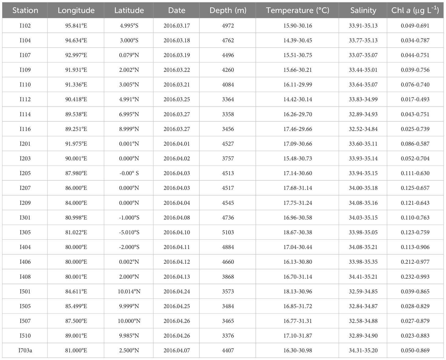
Table 1 Basic information of survey stations in the eastern Indian Ocean and variation range of general hydrological parameters (temperature, salinity, and integrated chlorophyll a) in the 0-200 m water column.
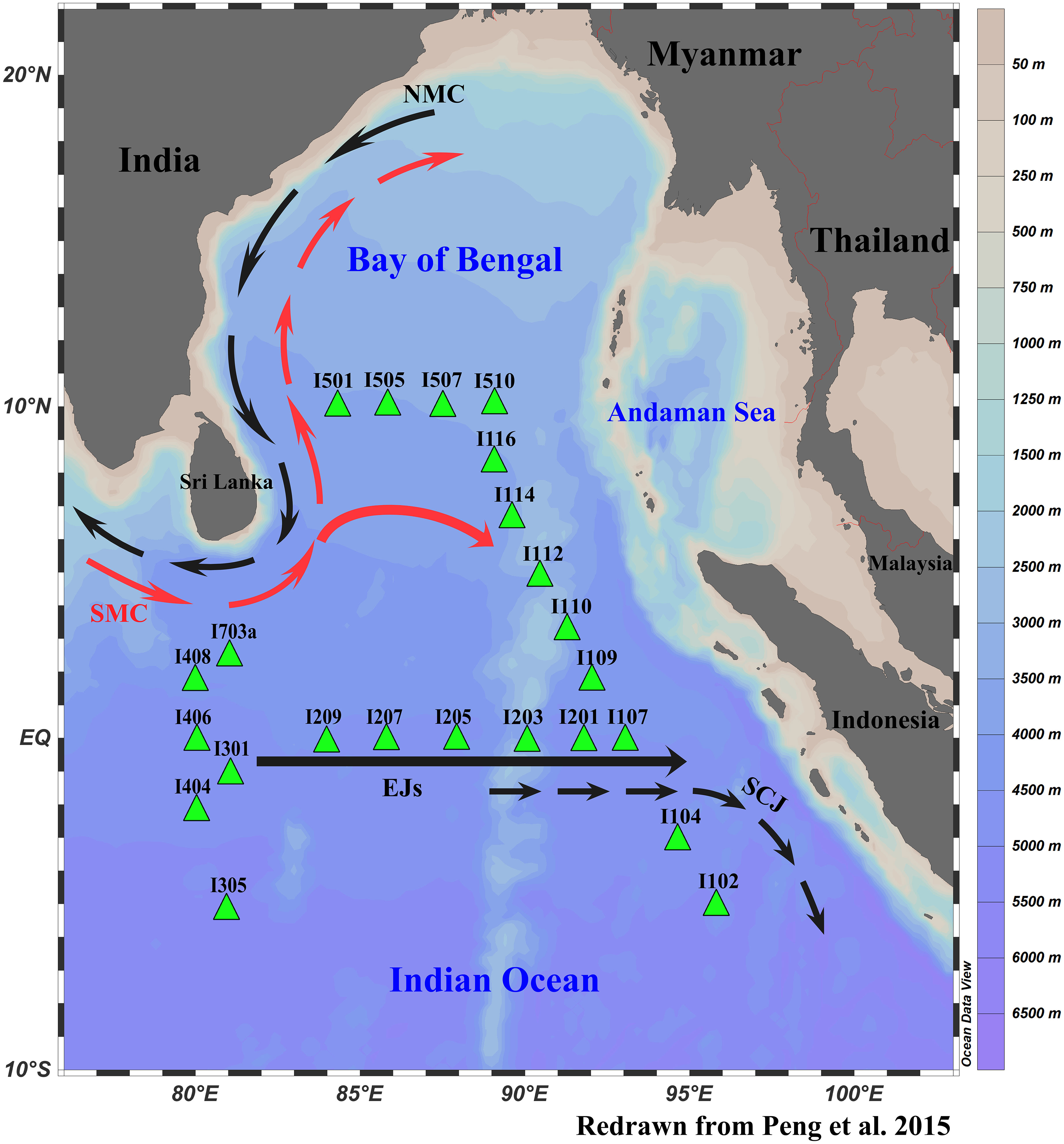
Figure 1 Location of microzooplankton sampling stations in the eastern Indian Ocean. The major surface currents include the Northeast Monsoon Currents (NMC), Southwest Monsoon Currents (SMC), Equatorial Jets (EJs, also called Wyrtki jets), and South Java Currents (SJC). The black (red) dotted arrows represent the occurrence of winter (summer), and the black straight arrows represent periodic occurrences in spring or autumn.
MZP samples were collected using a custom-made plankton net with a mesh aperture of 20 μm (80 cm mouth diameter, 0.5 m2 mouth area, total length 270 cm). A special digital flow meter (HYDRO-BIOS, Kiel) was set up to record the volume of the seawater column filtered by the plankton net. At each survey station, the vertically hauled net was lowered and recovered at the traction speeds of 0.5 m s-1 and 0.1 m s-1, respectively, a process which was carried out from a depth of 200 m to the surface. The collected samples were rinsed thoroughly with seawater filtered by Whatman GF/F glass filters and collected in 500 ml polyethylene plastic bottles. Then, the samples were fixed with 3% formaldehyde solution and stored in a dark place until the laboratory analysis.
The 100 ml seawater samples were collected and filtered through a 0.45 μm acetate fiber filter membrane. Then, the filtrate was refrigerated at 4°C and used for nutrient analysis. The concentrations of dissolved inorganic phosphorus (DIP), dissolved inorganic nitrogen (DIN), and dissolved silicon (DSi) were measured by the colorimetric method using an AA3 automatic analyzer (Bran Luebbe, Germany). The DIP in seawater was determined by the phosphorus molybdenum blue method (Martin and Doty, 1982) and the determination of DSi in seawater by the molybdenum blue method (Isshiki et al., 1991). The DIN measured included ammonium (NH4-N), nitrate (NO3-N), and nitrite (NO2-N). Ammonium was determined by the sodium salicylate method (Pai et al., 2001), nitrate was determined by the cadmium column method, and nitrite was determined by the naphthalene ethylenediamine method (Patey et al., 2008).
Then, 500 ml seawater samples of different depths (0.5 m, 25 m, 50 m, 75 m, 100 m, 150 m, and 200 m) were collected and filtered through a 20 μm mesh, a 2 μm cellulose acetate membrane, and a 0.2 μm Whatman-GF/F glass fiber filter membrane to obtain the concentration of size-fractionated chlorophyll a (micro-, nano-, and pico-). The total concentration of chlorophyll a was the sum of the concentrations of size-fractionated chlorophyll a. The filter membrane was wrapped in tin foil and stored in a refrigerator at -20°C for frozen preservation. In the laboratory, the membrane was extracted in 90% acetone solution for 24 h, after which the concentration of chlorophyll a was measured fluorometrically using a Turner Designs fluorometer (Hamilton, 1984). In this survey, the water depth, temperature, salinity, and other physical or chemical parameters were recorded by the Seabird CTD (Sea-Bird SCIENTIFIC, Seabird SBE 17 Plus) to understand the general hydrological situation of the sea area.
The MZP samples were slowly mixed and taken at 100 ml and gently filtered through a 200 μm mesh to remove a larger volume of plankton or impurities from the sample (Devi et al., 2020). Then, the filtrate was stored in 100 ml polyethylene bottles. Although the use of a mesh to filter samples may cause interference with some of the larger vulnerable MZP (Zhang et al., 2001), it can avoid covering or shielding other smaller MZP. In this way, can we avoid affecting the count and measurement of individual cells. Therefore, the filtration process is still widely used for plankton counting and identification (Liu et al., 2002; Jyothibabu et al., 2008a; Devi et al., 2010; Garzio et al., 2013).
The 100 ml filtrate sample was thoroughly mixed, and MZP subsamples (0.5ml-1ml) were taken by pipettors and placed in a 1 ml quantitative DSJ plankton counting frame. Species identification, individual counting, and linear parameter measurement were performed under a microscope (Motic Panthera L) at a magnification of 100-400X. For the species identification of MZP, we assumed that they were mainly heterotrophic, given that no chloroplasts were observed in the dinoflagellates group, purely autotrophic types of dinoflagellates are rare (Lessard and Swift, 1985), and heterotrophic or mixotrophic types are present in almost exclusively all dinoflagellates (Sun and Guo, 2011). This procedure has been adopted in many studies (Paterson et al., 2007; Jyothibabu et al., 2008b; Stoecker et al., 2014b; Yong et al., 2022). All tintinnids, including their empty lorica, were considered because the protoplast could easily dissociate from the lorica during sampling or after immobilization with chemical reagents (Gomez, 2007). Finally, we divided the MZP into five groups, namely, ciliates (CTS) including tintinnids and aloricate ciliates, heterotrophic dinoflagellates (HDS), copepod nauplii (CNP), sarcodines (SDS), and other taxa. Based on the available literature, CTS, HDS, and SDS were identified at the species level as far as possible, while CNP and other taxa were identified at the group level (Kofoid and Campbell, 1929; Kofoid and Campbell, 1939; Hada, 1970; Isamu, 1991; Tomas, 1997; Sun and Liu, 2002; Zhang et al., 2012).
According to the observed MZP individual geometry, the most approximate geometric model was selected, and the basic formula of the geometric model was used to calculate the MZP biovolume. The linear parameters of the volumetric model were measured using the ruler in the imaging system of the Motic Images Advanced 3.2 software. In routine analysis, it is not possible to measure the volume of each organism, and although some studies have shown that a minimum of 10 individuals per species is acceptable (Sun and Liu, 2003), we recommend measuring more individuals to obtain more accurate data. Therefore, we measured at least 20 independent individuals with complete traits for each species to calculate the biovolume of the species. The biovolume of each species was calculated from the mean linear parameter by a geometric formula (Hillebrand et al., 1999). For CTS, biovolume was measured according to the most similar geometry for each species, including cylinder, cone, and sphere, etc. Measurements of carbon biomass of tintinnids based on lorica volume tend to be overestimated (Gilron and Lynn, 1989). Therefore, the measurement of linear parameters should not include the thickness of the lorica but should be based on the actual space of protoplasts within the lorica as the volume used for carbon biomass calculation. In addition, the volume of the protoplast should be calculated as 1/3 of the volume of the space in which the protoplast may exist (Rychert, 2011). These measurements can be employed to try to avoid overestimating the carbon biomass of CTS protoplasts. The volume of HDS was measured by referring to the volume model of Sun (Sun and Liu, 2003). The volume of SDS was measured according to the method described by Caron (Caron et al., 1995), and the basic trait parameters, such as body length, were measured for CNP (Uye et al., 1996).
The carbon biomass of MZP is usually calculated using a conversion factor combined with the volume of individual organisms (Putt and Stoecker, 1989; Sun et al., 2007; Stoecker et al., 2014b; Wang et al., 2022). Based on the existing literature, we used conversion factors to calculate carbon biomass for tintinnids (0.053 pg C μm-3) (Verity and Lagdon, 1984), heterotrophic dinoflagellates (0.76 pg C μm-3) (Menden-Deuer and Lessard, 2000), and sarcodines (0.0026 pg C μm-3 for radiolarians and 0.018-0.18 pg C μm-3 for foraminiferans) (Caron et al., 1995). The carbon biomass of copepod nauplii was calculated using an empirical formula for body length (Uye et al., 1996). However, other taxa were not measured for carbon biomass because they were not common or had very low abundance in the samples. For each sample, we calculated the abundance and carbon biomass of MZP by estimating the total number of MZP individuals in the sample divided by the volume of the filtered water column at the sampling depth.
The average temperature, average salinity, and average integrated chlorophyll a concentration in the sampling water column were calculated by trapezoidal integration (Uitz et al., 2006).
Where PT, PS, and PC are, respectively, the average temperature (°C), average salinity, and average integrated chlorophyll a concentration (μg L-1) in the sampling water column; Pi is temperature, salinity, or integrated chlorophyll a concentration in layer i; D is the maximum depth (m) of the sampled water column; Di is the depth (m) of water layer i; and n is the sampling level in the water column.
The abundance of population is the most basic form of data for understanding the community structure of MZP, but there are relatively few studies on carbon biomass due to the different types of fixatives, the choice of volume model, and conversion factors (Yang et al., 2008; Stoecker et al., 2014b). In this study, the abundance and carbon biomass were calculated according to the following formulae:
Where A is the total abundance (ind. m-3) of MZP in a sample; N is the individual number of MZP in a subsample examined under a microscope; V1 is the volume (ml) of the subsample; V2 is the volume (ml) of the net sampling sample; and V3 is the volume (m3) of the filtered water column.
Where B is the total biomass (μg C m-3) of MZP in a sample; C is the carbon biomass of MZP in a microscopic subsample; V1 is the volume (ml) of the subsample; V2 is the volume (ml) of the net sampling sample; and V3 is the volume (m3) of the filtered water column.
The dominance of MZP and their various groups was calculated using the following formula (Xu and Chen, 1989):
Where Y is the dominance of the species i; ni is the individual number of the species i; N is the total individual number of MZP; and fi is the frequency of occurrence of the species i.
The biodiversity index is an important indicator for evaluating and judging the diversity of biological community structure or ecosystem stability (MacArthur, 1955).To analyze the diversity level of MZP and their major group communities, we used the following biodiversity indices.
The Margalef index (d) was used to calculate the species richness index (Abrams, 1989):
Where d is the Margalef richness index; S is the species number of MZP in the sample; and N is the individual number of MZP in the sample.
The Shannon–Weaver diversity index (H’) with base 2 was used to calculate the species diversity index (Shannon, 1950):
Where H’ is the Shannon–Weaver diversity index; S is the species number of MZP in the sample; Pi = (ni N-1) is the ratio of individual of the i species to the total individual number of MZP in the sample; and N is the total individual number of MZP in the sample.
The Pielou evenness index was used to calculate the species evenness index (Pielou, 1966):
Where J is the Pielou evenness index and S is the species number of MZP in the sample.
In this study, the data of biological variables (abundance and carbon biomass) and environmental parameters (temperature, salinity, chlorophyll a) were graphed and analyzed by Ocean Data View 5.5.2 and Origin pro2022. The biodiversity index of MZP and their major groups was calculated by Past 4.09. Correlation analysis of the data was performed by IBM SPSS Statistics 27. Cluster analysis was used to reflect the differences in MZP communities, and Primer 6 (6.1.12.0) was used for data visualization.
Through the observation of the basic hydrological parameters (temperature, salinity, and integrated chlorophyll a) at 23 survey stations (Table 1), it can be seen that the average temperature, average salinity, and average integrated chlorophyll a concentration in the eastern equatorial Indian Ocean show obvious spatial differences during the spring intermonsoon (Figure 2). On the spatial distribution, the changes of each hydrological parameter showed a trend of high value in the west and low value in the east. At all stations, the temperature of the surface seawater ranged from 29.66 to 31.87°C, the average temperature of the water column ranged from 23.21 to 27.25°C (mean of 25.29 ± 0.89°C), the salinity of the surface seawater ranged from 32.38 to 34.41, the average salinity of the water column ranged from 33.37 to 34.95 (mean of 34.39 ± 0.45), and the average integrated chlorophyll a concentration of the water column ranged from 0.2328 to 0.526 μg L-1 (mean of 0.3689 ± 0.0688 μg L-1). There were large temperature variations between all stations, with the maximum average temperature (27.25°C) occurring at station I406 and the minimum average temperature (23.21°C) occurring at station I112, while the temperature changed relatively gently among the other stations and did not change significantly at the horizontal gradient of latitude. In terms of general trends, the temperature was relatively low in the offshore transect along the west coast of Sumatra, while the temperature of seawater was relatively high in the mouth of the Bay of Bengal and the western part of the eastern Indian Ocean. The range of salinity chance in the eastern equatorial Indian Ocean area was relatively small, with the maximum value (34.95) appearing at station I408 and the minimum value (33.37) appearing at station I510, but the salinity showed an obvious gradient in the latitude direction. In the equatorial transect, the salinity of the seawater was maintained at a relatively high level, and the salinity variation between the stations was small. Therefore, the salinity distribution of the transect zone showed a stable state (Figure 2B). However, the salinity of the seawater in the Bay of Bengal in the transect 10°N north of the equator was relatively low, which presented an obvious difference boundary with the salinity of the seawater near the equator. The seawater with a high concentration of integrated chlorophyll a was mainly distributed in the western part of the eastern Indian Ocean, while the integrated chlorophyll a in the eastern part of the sea was relatively low. The distribution of chlorophyll a was the same as that of temperature, with the minimum value appearing at station I112 and the maximum value appearing in the western waters of the eastern Indian Ocean. This indicates that there may be a strong similarity between the distribution pattern of integrated chlorophyll a and that of temperature. The concentration of size-fractionated chlorophyll a had a significant bias in the proportion of total chlorophyll a concentration, among which the concentration of nano-chlorophyll a occupied the highest proportion of 50.5%, followed by the concentration of pico-chlorophyll a occupying 45.5% and the concentration of micro-chlorophyll a occupying only 4%.
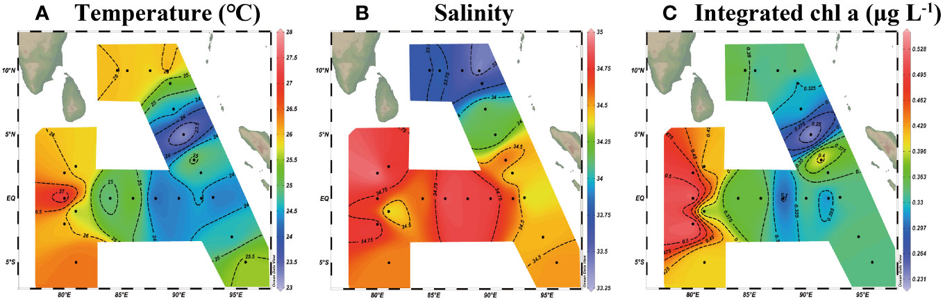
Figure 2 Spatial distribution of (A) temperature (°C), (B) salinity, and (C) integrated chlorophyll a concentration (μg L-1) in the eastern Indian Ocean during the spring inter-monsoon.
By analyzing MZP samples collected from 23 stations in the eastern equatorial Indian Ocean, we identified MZP belonging to 2 phyla (Protozoa and Arthropoda), 63 genera, and a total of 340 species (Supplementary Material Table 1). The level of species composition and proportion of each biological group in all survey stations were as follows (Figure 3). HDS contributed from 22 genera and 206 species (1 unidentified species) accounted for 59.4% of the total species number of MZP. CTS contributed from 36 genera and 126 species (1 unidentified species) accounted for 36.5% of the total species number. It is seen that the genus number of CTS was larger, while the species number of HDS was larger. Among HDS, Ceratium accounted for the largest number of species (54 species) and accounted for 26.34% of the total species number of HDS, followed by Dinophysis and Protoperidinium (20 species each), which accounted for 9.76% of the total species number of HDS; this may indicate that Ceratium has more selectivity in environmental adaptation. Among CTS, Eutintinnus species were the most abundant (13 species), accounting for 10.32% of the total species number of CTS, followed by Salpingella (10 species), accounting for 7.94%, and thirdly by Rhabdonella (9 species), which accounted for 7.14%. In addition, the presence of symbiosis with other phytoplankton (Synechococcus and Ornithocercus) in HDS algal cells was noted in our specific observations of individual organisms, and most of the tintinnids were hyaline species in which a portion of the cellular protoplasts had escaped from the lorica.
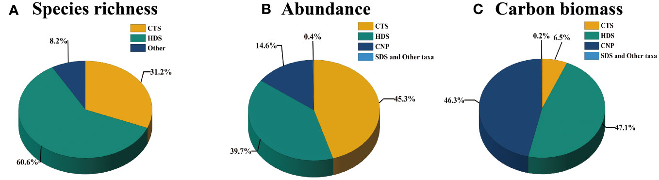
Figure 3 The composition proportion of (A) species richness, (B) abundance, (C) carbon biomass of the microzooplankton community in the eastern Indian Ocean.
In all sampling stations in the eastern equatorial Indian Ocean, the MZP abundance ranged from 701 to 9235 ind. m-3 (mean of 2588 ± 1767 ind. m-3). The abundance of CTS ranged from 234 to 4400 ind. m-3 (mean of 1173 ± 912 ind. m-3) and accounted for 45.3% of the total abundance of MZP (Figure 3B). The abundance of HDS ranged from 234 to 3650 ind. m-3 (mean of 1029 ± 725 ind. m-3) and accounted for 39.7% of the total abundance of MZP. The abundance of CNP ranged from 125 to 1106 ind. m-3 (mean of 379 ± 207 ind. m-3) and accounted for 14.6% of the total abundance of MZP. SDS and other taxa were fewer in this study, with a range of 0-79 ind. m-3 (mean of 9 ± 17 ind. m-3) and the total abundance accounting for only 0.4%. The MZP community in the eastern equatorial Indian Ocean was mainly contributed by CTS and HDS, which shared the same characteristics of abundance and species diversity. In addition, CNP also occupied a certain proportion of abundance in each sample, which was much higher than that of SDS and other groups.
The carbon biomass of MZP ranged from 8.013 to 83.678 μg C m-3 (mean of 28.576 ± 15.69 μg C m-3). The carbon biomass levels of HDS ranged from 2.033 to 57.94 μg C m-3 (mean of 13.459 ± 11.734 μg C m-3) and accounted for 47.1% of the total carbon biomass of MZP (Figure 3C). The carbon biomass of CNP ranged from 3.524 to 30.496 μg C m-3 (mean of 13.245 ± 6.35 μg C m-3) and accounted for 46.4% of the total carbon biomass. The carbon biomass of CTS ranged from 0.46 to 6.768 μg C m-3 (mean of 1.847 ± 1.312 μg C m-3) and accounted for 6.5%. The carbon biomass of SDS and other taxa was very low and accounted for only 0.2% of the total carbon biomass.
There were significant differences in the species richness levels of MZP among all the stations in the eastern equatorial Indian Ocean. The maximum number of MZP species (179 species) appeared at station I110, of which 101 species were mainly contributed by HDS. The minimum number (52 species) appeared at station I112, of which 29 species were mainly contributed by CTS. These results indicated that HDS dominated the MZP community when species richness was high, while CTS might have been more dominant when species richness was low. However, the locations of the maximum and minimum species numbers of CTS and HDS were not synchronized. The maximum (71 species) and minimum (22 species) number of CTS species occurred at stations I110 and I501, respectively. It may be that environmental factors such as temperature have a certain impact on the traits of organisms, resulting in differences in species diversity. The maximum (102 species) and minimum number (17 species) of HDS species occurred at stations I104 and I112, respectively.
Figure 4 represents the spatial variability in abundance and carbon biomass distribution of MZP and the major groups (CTS and HDS). The total abundance of MZP showed that the coastal area was a high abundance area, while the abundance of MZP in the open ocean far from the coast was relatively low (Figure 4A). MZP are the main predators of phytoplankton (such as cyanobacteria or diatoms) in oligotrophic waters at low latitudes, so the distribution pattern of food may affect the distribution of predators. Relatively high concentrations of chlorophyll a in coastal waters indicate high phytoplankton densities in this area, which may cause a proliferation of MZP. At the same time, the maximum abundance of MZP in the survey area appeared at station I110 (9235 ind. m-3), but there was a big difference in MZP abundance in the nearby station I112 (967 ind. m-3). Combined with the results of minimum values of temperature (Figure 2A) and integrated chlorophyll a concentration (Figure 2C) at station I112, we believe that when the average temperature of each water layer in the eastern equatorial Indian Ocean attains a low-temperature condition of about 23°C, the bloom of the phytoplankton and MZP community will be severely restricted. In addition, the distribution pattern of the total abundance of MZP was similar to that of CTS and HDS (Figures 4B, C), indicating that the MZP community in the eastern Indian Ocean was mainly dominated by CTS and HDS. At the same time, the abundance ratio of CTS and HDS showed that CTS may make a greater contribution to the regulation of the abundance structure of the MZP community.
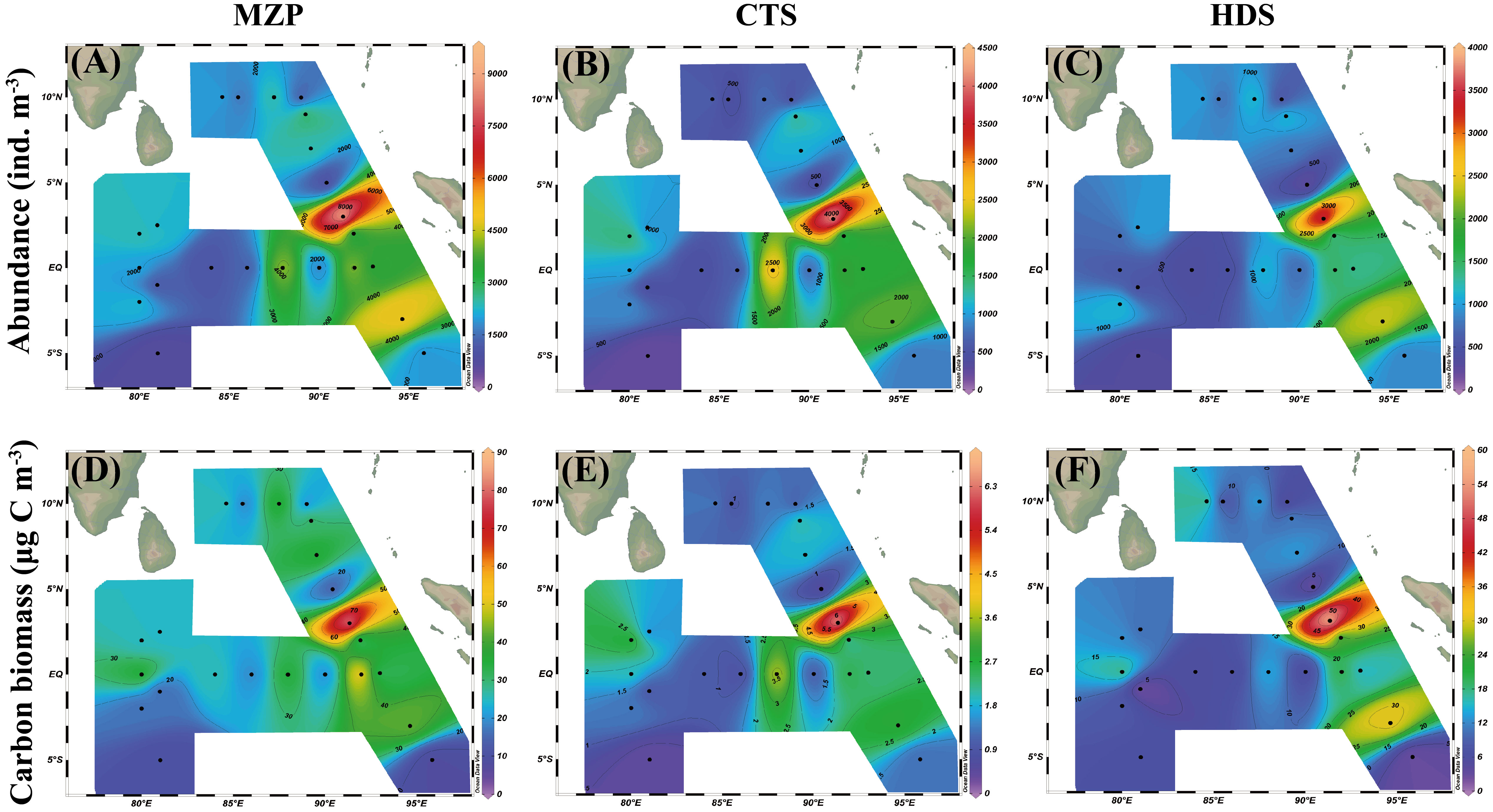
Figure 4 Spatial distribution of (A–C) abundance (ind. m-3) and (D–F) carbon biomass (μg C m-3) of microzooplankton and their major groups in the eastern Indian Ocean.
In terms of carbon biomass, the maximum value of the carbon biomass of the MZP appeared at station I110 (83.678 μg C m-3), and the minimum value appeared at station I102 (8.013 μg C m-3) (Figure 4D). In addition, the carbon biomass of MZP in the waters south of the equator was low. In the seawater north of the equator, except for station I110, the carbon biomass of MZP in other stations was more evenly distributed with little difference. The high carbon biomass sea areas of CTS and HDS mainly appeared in the coastal waters of the west coast of Sumatra (Figures 4E, F), but the carbon biomass levels were generally low. The carbon biomass distribution patterns of CTS and HDS were different from those of MZP, possibly because a large proportion of the carbon biomass of MZP in the eastern Indian Ocean was contributed by CNP. Therefore, in the various MZP groups, HDS and CNP may have stronger organic carbon storage capacity than CTS. It could also be because the measurement standard of volume size and the selection of conversion factor could affect the estimation of the carbon biomass of MZP.
The magnitude of dominance often reflects the role and ecological position of the species population in the biological community. The species composition of the top 9 dominant species of MZP in the eastern equatorial Indian Ocean (Table 2, Figure 5), the proportion of abundance of each species in the dominant species group (Figure 6), and the spatial distribution of abundance of each dominant species (Figure 7) were shown in the chart. The dominant species of MZP in the eastern Indian Ocean seawaters consisted mainly of CTS (6 species) and HDS (3 species), with the dominant species of CTS occupying a greater proportion of the abundance level than the dominant species of HDS (Figure 6). CNP were present at all stations and occupied a large proportion of the abundance (Figure 2B). These results may indicate that CNP, CTS, and HDS are eurytopic organisms among the dominant groups of MZP in the eastern Indian Ocean, and CNP may also play an important role in the microbial food web. CNP were abundant in the seawater of the eastern equatorial Indian Ocean. In the 0-200 m water layer of the eastern equatorial Indian Ocean, the abundance of CNP ranged from 126 to 1106 ind. m-3 (mean value of 379 ind. m-3). The population abundance of CNP accounted for 14.6% of the total abundance of MZP, and the maximum population abundance (1106 ind. m-3) was observed at station I110. Copepods are permanent zooplankton, and their larval populations are also considerable and widely distributed, so they are known as one of the largest biomasses of multicellular organisms in the world’s oceans.
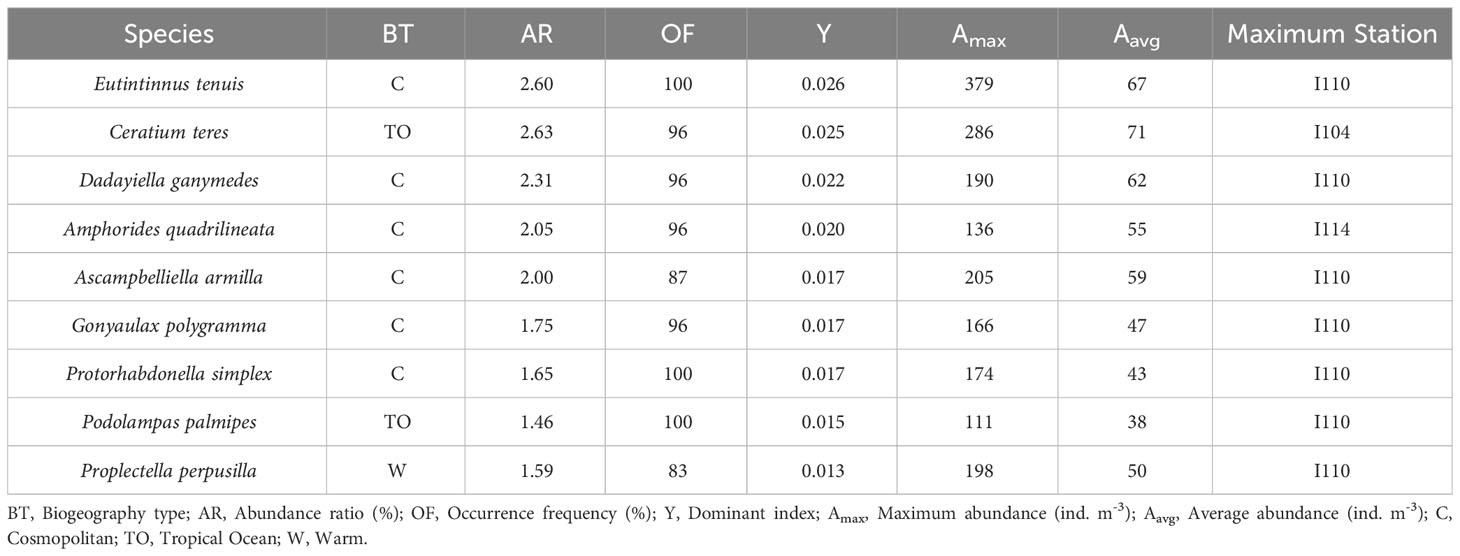
Table 2 Dominant species of microzooplankton in the eastern Indian Ocean and related statistics.
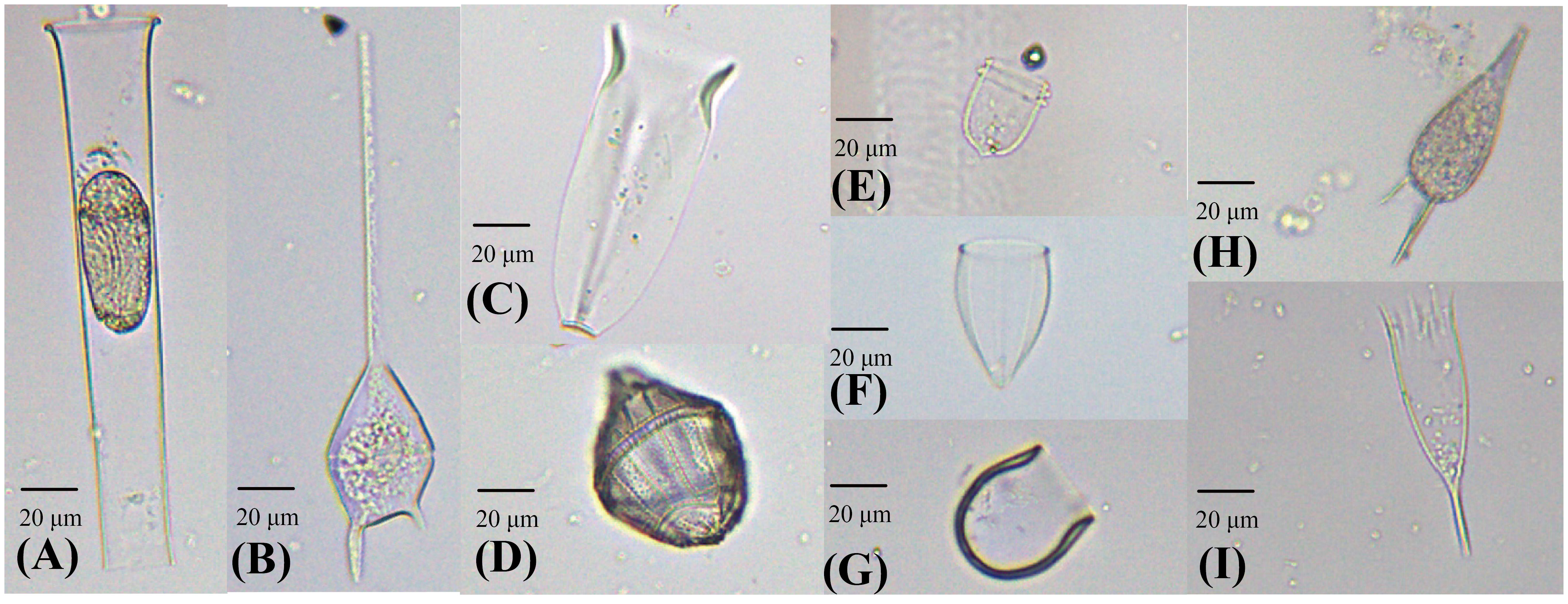
Figure 5 Photographs of dominant species in the eastern Indian Ocean. (A) Eutintinnus tenuis; (B) Ceratium teres; (C) Amphorides quadrilineata; (D) Gonyaulax polygramma; (E) Ascampbelliella armilla; (F) Protorhabdonella simplex; (G) Proplectella perpusilla; (H) Podolampas palmipes; (I) Dadayiella ganymedes.
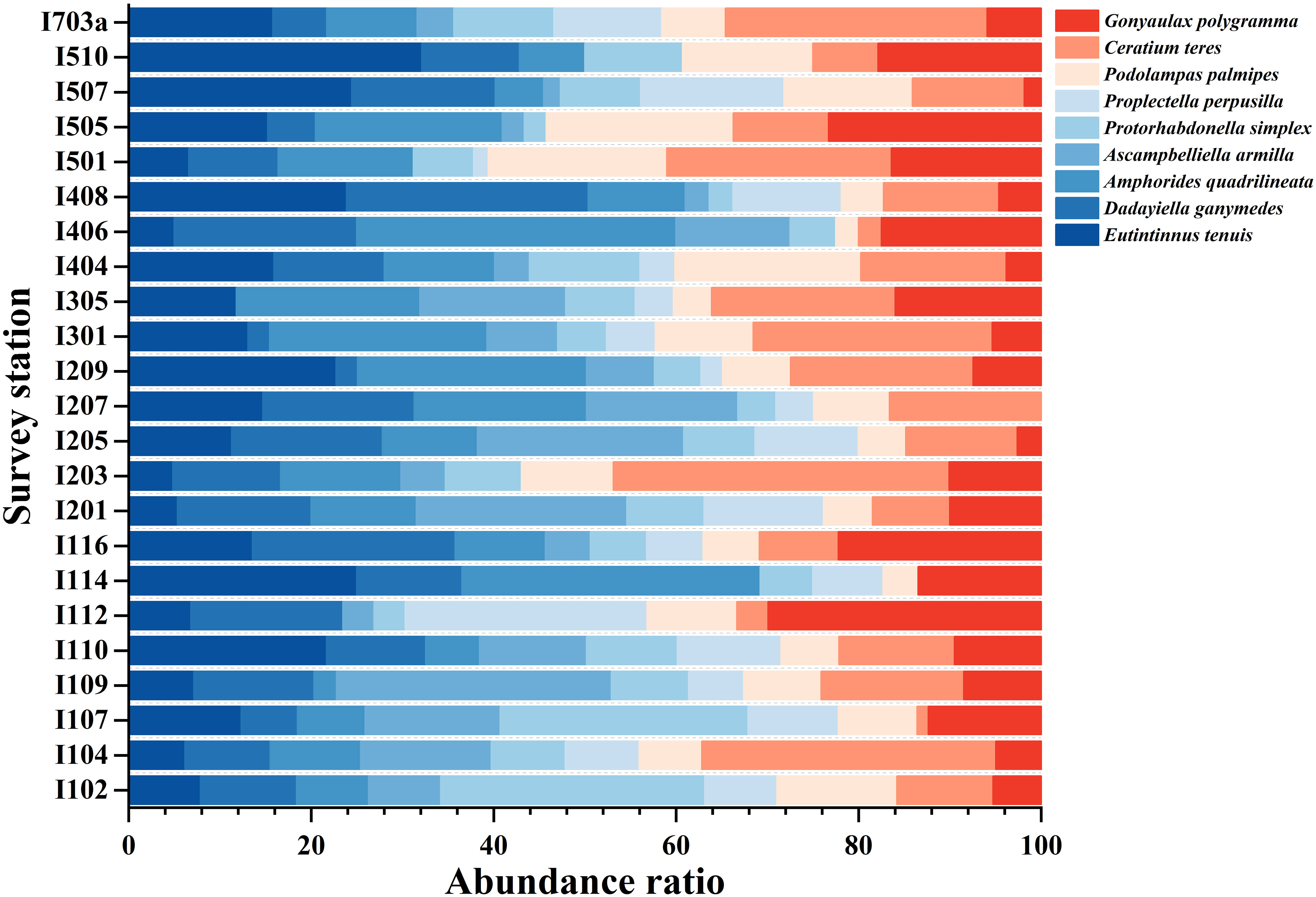
Figure 6 Abundance ratios of dominant species of microzooplankton in the eastern Indian Ocean. The blue line is the ciliates group; the light red is the heterotrophic dinoflagellates group.
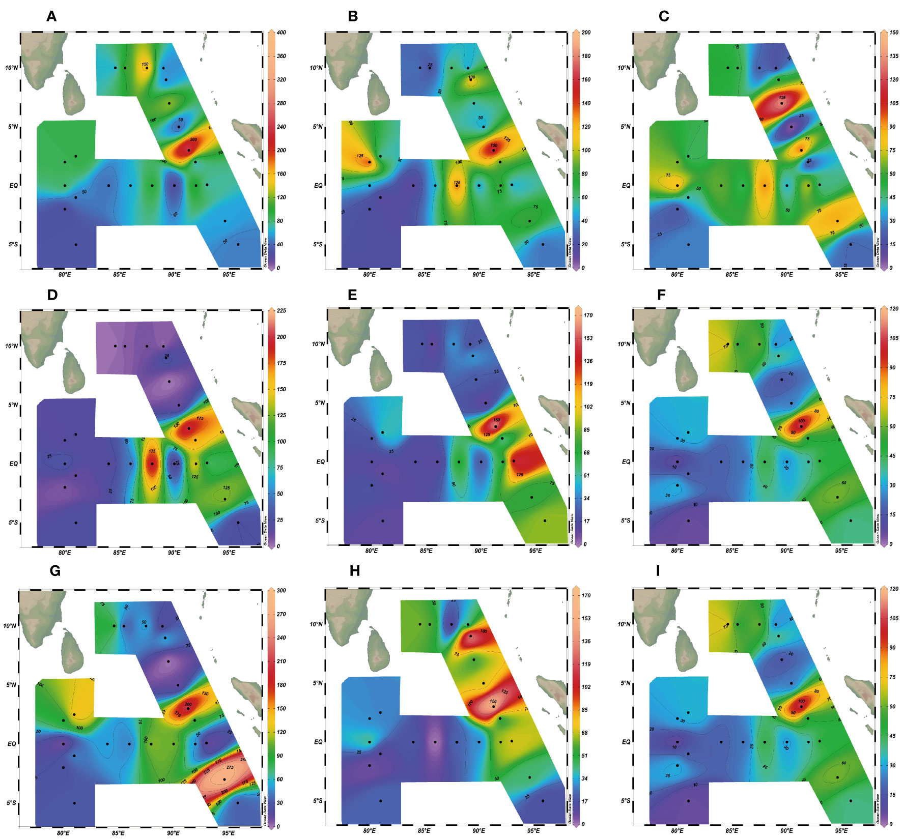
Figure 7 Spatial distribution of the abundance (ind. m-3) of dominant species of microzooplankton in the eastern Indian Ocean. (A) Eutintinnus tenuis; (B) Dadayiella ganymedes; (C) Amphorides quadrilineata; (D) Ascampbelliella armilla; (E) Protorhabdonella simplex; (F) Proplectella perpusilla; (G) Ceratium teres; (H) Gonyaulax polygramma; (I) Podolampas palmipes.
According to Table 2, among the CTS group, the most dominant species was Eutintinnus tenuis (Y=0.026) (Figure 7A), followed by Dadayiella ganymedes (Y=0.022) (Figure 7B). Tintinnids have protective lorica, and since their feeding is limited by the lorica oral diameter (LOD), generally, the optimal food size for CTS is generally about 25% of the LOD (Dolan et al., 2013a). Compared with lorica length (LL), the change rangeability in LOD of CTS is smaller; thus, LOD usually is a more stable and reliable trait of CTS in species identification. In this investigation, the LOD of E. tenuis ranged from 35 to 45 μm and LL from 180 to 220 μm (Supplementary Material Table 1). E. tenuis was found in all survey stations and widely distributed so that it often belonged to a cosmopolitan species in biogeography. The abundance of E. tenuis ranged from 12 to 379 ind. m-3 (mean value of 67 ind. m-3), accounting for 2.6% of the MZP community. The maximum population abundance occurred at station I110 (379 ind. m-3) and accounted for 4.1% total abundance of the MZP at the station.
Among the HDS group, the most dominant species was Ceratium teres (Y=0.025) (Figure 7G), followed by Gonyaulax polygramma (Y=0.017) (Figure 7H) and Podolampas palmipes (Y=0.015) (Figure 7I). The occurrence rate of C. teres was 96% at the survey stations and was not observed only at station I114. This species was found in many typical marine areas of the world, mainly in tropical seawaters with high temperature, and it belonged to the tropical zone oceanic species in biogeography. At all survey stations, the abundance of C. teres ranged from 6 to 286 ind. m-3 (mean value of 71 ind. m-3), and its abundance of population accounted for 2.63% of the total abundance of MZP. The maximum abundance of C. teres was found at station I104 (286 ind. m-3) and accounted for 5.9% of the MZP abundance at the station. The occurrence rate of G. polygramma was 96% at the survey stations and was not observed only at station I207. G. polygramma was a widely distributed species, with abundance ranging from 6 to 166 ind. m-3 (mean value of 47 ind. m-3). The maximum abundance was observed at station I110 (116 ind. m-3), which accounted for 1.8% of the MZP abundance at the station. The occurrence rate of P. palmipes in the survey station was 100%, and it also belonged to the tropical zone oceanic species in biogeography. The abundance of P. palmipes ranged from 6 to 111 ind. m-3 (mean value of 38 ind. m-3), accounting for 1.46% of the total abundance of MZP. The maximum abundance of P. palmipes was found at station I110 (111 ind. m-3) and accounted for 1.2% of the MZP abundance at the station.
We used the Margalef richness index (d), Shannon–Weaver diversity index (H'), and Pielou evenness index (J) to comprehensively describe and analyze the diversity of the MZP community structure in the equatorial eastern Indian Ocean (Table 3; Figure 8). The d of MZP ranged from 10.58 to 25.2 (mean value of 18.25 ± 3.56), H’ ranged from 5.1 to 6.7 (mean value of 6.1 ± 0.4), and J ranged from 0.88 to 0.95 (mean value of 0.91 ± 0.02). The maximum richness index and species diversity index of the MZP community were located at station I110 (Figure 8), and a total of 179 species of MZP were found at this station, followed by station I104 with 167 species. The levels of biodiversity indices were similar between the two stations, and the general changing trends of MZP and HDS were more similar in the two stations (Figure 8). This indicates that the diversity of the MZP community is mainly determined by the dominant HDS when the richness of MZP community is high. In addition, the two stations were similar in that they were both stations with the maximum abundance of HDS dominant species (Table 2), but the difference was that there was a significant discrepancy in the abundance of MZP at the two stations, among which the population abundance of I104 station was only 52% of the I110 station. This may indicate that the stability degree of MZP community in the two stations is similar, while the environmental carrying capacity of the two stations is significantly different. Station I112 had a low level of MZP community diversity with low abundance and carbon biomass, while the neighboring station I110 had a high level of diversity. The differences in species diversity indices of the MZP community among other stations were small. As for the evenness of the community, the difference in the evenness index at each station was not large in terms of distribution, and the evenness index also showed no obvious distribution pattern (Figures 8C, F, I).
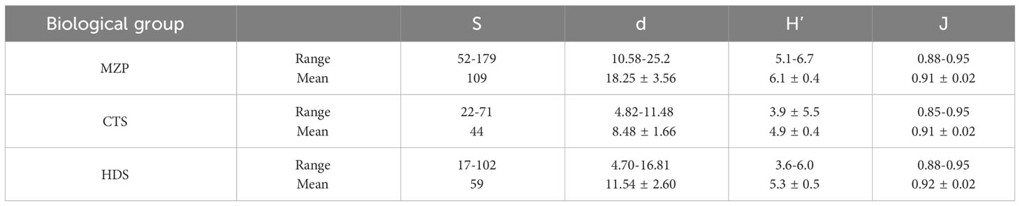
Table 3 Biodiversity indices (S, Species richness; d, Margalef richness index; H’, Shannon–Weaver diversity index; J, Pielou evenness index) of microzooplankton and their major groups.
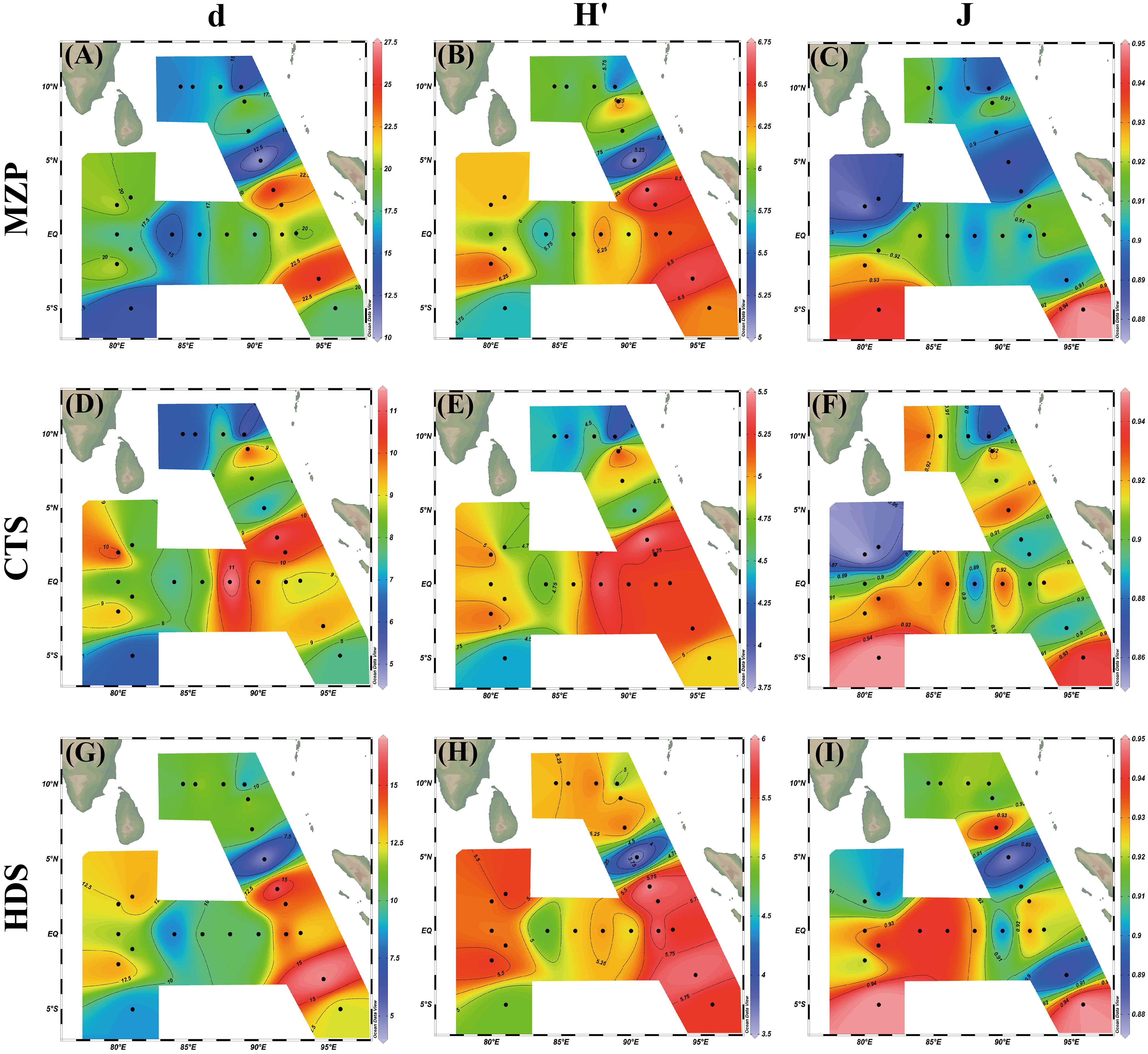
Figure 8 Spatial distribution of biodiversity indices of microzooplankton and its major groups. (A–C) are Margalef richness index (d), Shannon–Weaver diversity index (H’), Pielou evenness index (J) for total microzooplankton, respectively, (D–F) are Margalef richness index (d), Shannon–Weaver diversity index (H’), Pielou evenness index (J) for ciliates, (G–I) are Margalef richness index (d), Shannon–Weaver diversity index (H’), Pielou evenness index (J) for heterotrophic dinoflagellates.
When the environment is relatively stable, the biological communities in different regions tends to have a relatively high species composition similarity. Although there are usually no clear boundaries between different communities, they can still be distinguished after analysis. According to the species diversity and abundance of MZP in the 200 m water column at each sampling station, our study divided MZP in the eastern equatorial Indian Ocean roughly into five biological groups and completed the clustering analysis via Bray–Curtis similarity (about 50%) (Figure 9). Except station I112, the similarity of the MZP community in other stations was more than 40%. The maximum Bray–Curtis similarity between the stations was about 63%, and most other stations were 50%-60%. Among them, station I112 had a low similarity with other stations and was divided into group 1, which was consistent with our other analysis results. Combined with the analysis of environmental factors, the division of this community may be mainly influenced by the occurrence of lower temperatures in I112. I305 and I510 were divided into group 2, while I207 and I209 were divided into group 3. The average abundance of MZP in group 2 was 1240 ind. m-3, and CNP and A. quadrilineata occupied a large proportion in the abundance level of the community. Group 4, marked in blue, covered 47.8% of the survey stations, indicating that the basic characteristics of this group may represent the main situation of the MZP community in the survey area. Group 5, marked in orange, also covered a large proportion of the survey stations (30.4%).
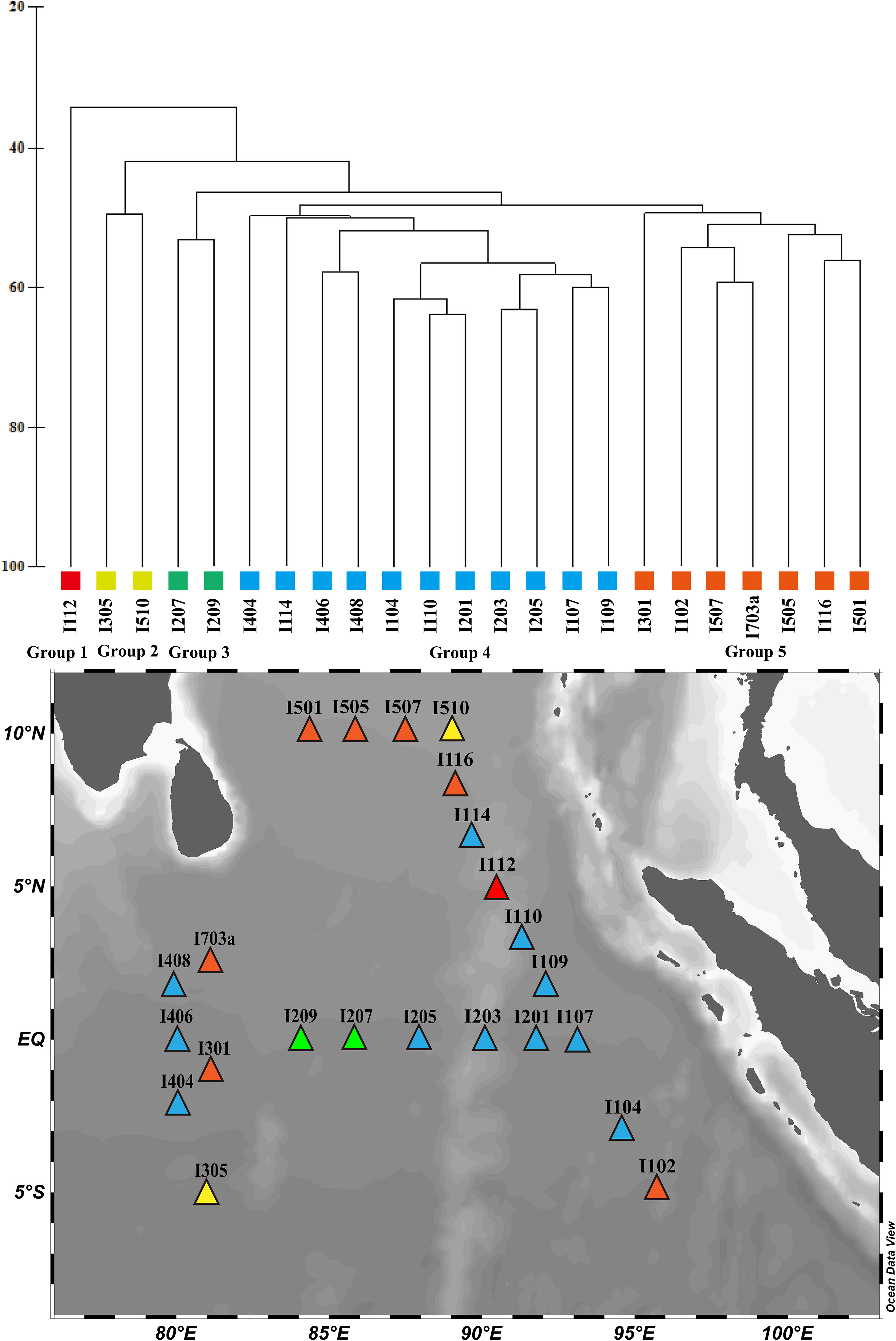
Figure 9 Cluster analysis of microzooplankton communities in the eastern Indian Ocean.
Understanding the characterization of changes in hydrological parameters in the eastern Indian Ocean may help us find the survival mechanism of MZP adapting to an oligotrophic environment. We can see that the temperature changes in the eastern equatorial Indian Ocean are much more pronounced than the salinity (Figure 2A). Because the eastern Indian Ocean is an important part of the Indian ocean–Pacific warm pool (Schott et al., 2009), and the sea surface temperature of the eastern Indian Ocean warm pool is very significantly affected by the heat flux of the sea surface (Lin et al., 2014), it is thus easily subject to interference and change, such as water mass blend, solar radiation intensity, and degree of cloud cover, etc. (Wiggert et al., 2006). Cooler seawater occurs off the west coast of Sumatra, while the Bay of Bengal’s mouth and the western part of the eastern Indian Ocean have relatively warmer waters. This may be due to the start occurrence of the southwest monsoon and the northeast monsoon fading away during the spring intermonsoon period. Therefore, the west coast of Sumatra may still be under the influence of the low-temperature NMC, but this influence is diminishing and being replaced by the warm SMC. In the comparison of the variation amplitude of temperature distribution in the longitude horizontal direction and latitude horizontal direction, it can be seen that the variation difference of temperature in the longitude direction is more prominent. This is likely due to the eastward advance of the Wyrtki jets (EJs) that are driven by equatorial west wind drifts during the spring intermonsoon, which mixes high-temperature water in the western Indian Ocean with relatively low-temperature seawater in the east (Wyrtki, 1973). These may indicate that in a short time series, the intrusion of currents has a more severe impact on the temperature distribution pattern in the eastern equatorial Indian Ocean.
In the equatorial transect, the salinity of seawater varies relatively little and is kept at a relatively high level, but there is a boundary where the salinity changes dramatically due to the convergence of water masses with different characteristics. The salinity in the spatial distribution shows obvious latitudinal changes (Figure 2B), and the salinity of the seawater at the mouth of the Bay of Bengal is relatively low and shows a clear boundary at 7°N. This phenomenon is mainly because the Bay of Bengal is the largest semi-enclosed bay in the world, with annual concentrated precipitation, sufficient runoff freshwater input, and weak seawater evaporation. This indicates that the salinity levels in the two transects are affected by water masses with different characteristics. At the smaller latitudes range, there is a boundary where the salinity of the sea changes dramatically, which may be caused by the intrusion of the current or water mass. Combining with Peng et al.’s analysis of ocean current distribution in the Indian Ocean (Peng et al., 2015), the dramatic changes in salinity at this latitude are more likely caused by the branch (Figure 1) of the weaker SMC at the mouth of the Bay of Bengal during the spring intermonsoon period as SMC gradually intensifies. This branch of the current driven by the southwest monsoon gradually invades the Bay of Bengal, carrying the high salinity seawater of the Arabian Sea from the western Indian Ocean. However, due to the gradual increase of spring intermonsoon rainfall in the Bay of Bengal and the abundant surface runoff into the bay causing stratification of the seawater in the bay (Kumar et al., 2002), the salinity of the Bay of Bengal is relatively low, and it is in an oligotrophic state. Finally, the salinity boundary is formed at the mouth of the Bay of Bengal, which shows that the salinity of the seawater in the bay to the north of the mouth of the bay is relatively low, and the salinity of the seawater in the south of the mouth of the bay is maintained in a state of high salinity.
The spatial distribution of integrated chlorophyll a show a high value in the western seawater and a low value in the eastern coastal seawater, especially in the equatorial transect (Figure 2C). This may be mainly due to the periodic occurrence of Wyrtki jets along the eastern Indian Ocean equator during the spring intermonsoon period. Driven by the equatorial west winds drifts, this current originates in the western Indian Ocean and carries the high temperature and high salt seawater of the Arabian Sea eastward to push into the oligotrophic eastern Indian Ocean (Wyrtki, 1973), thus providing better growth conditions for phytoplankton in western seawater in the eastern Indian Ocean and enabling a high value of integrated chlorophyll a concentration to appear in the sea area. The distribution characteristics of chlorophyll a in the eastern equatorial Indian Ocean showed a more significant correlation with the distribution of temperature (Figures 2A, C). Pearson’s correlation analysis (Figure 10) proved that integrated chlorophyll a concentration is significantly positively correlated with temperature (R=0.748, P=0.00004<0.01, n=23) and salinity (R=0.420, P=0.046<0.05, n=23). However, compared with salinity, the integrated chlorophyll a concentration has a stronger correlation with temperature, and this analysis result is consistent with the results shown by its distribution pattern. This may indicate that temperature is the main environmental factor affecting phytoplankton growth in the equatorial eastern Indian Ocean, and the feature of such distribution may be caused by the alternating strength of the Indian monsoon during the spring intermonsoon. In addition, through the analysis of the size-fractionated chlorophyll a concentration, we can see that the proportion of phytoplankton with smaller algal cell diameter is larger in the sea area. This shows that phytoplankton with smaller algal cell diameter (nanophytoplankton and picophytoplankton) may dominate the contribution to primary production in the low-latitude oligotrophic eastern Indian Ocean. This may be due to the larger cell surface area-to-volume ratio of phytoplankton with smaller algal cell diameter, which allows them to absorb the required nutrients more efficiently to adapt to the environment (Uitz et al., 2006). This result is similar to the research results of Calbet and Landry on MZP feeding in oligotrophy sea areas (Calbet and Landry, 1999), and this is in accord with the characteristics of MZP preferentially selective feeding (Evelyn and Barry, 2007). This may be evidence that in tropical oligotrophic oceans, the boom of smaller phytoplankton communities leads to the expansion of the MZP community (Caron and Hutchins, 2012).
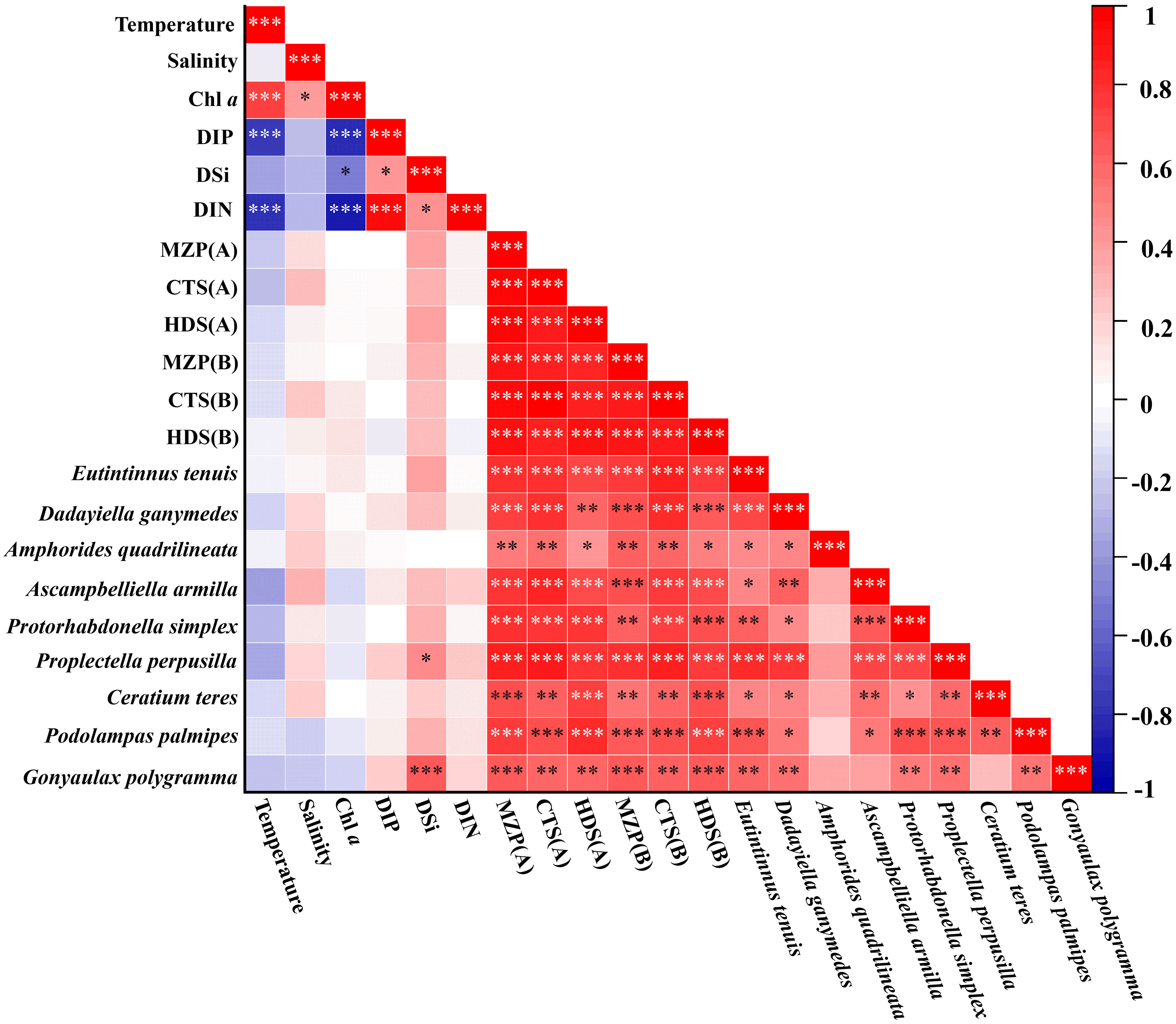
Figure 10 Correlation analysis of biological variables and environmental factors of microzooplankton. (A) Abundance; (B) Biomass; *, a significant correlation at the 0.05 confidence level; **, a significant correlation at the 0.01 confidence level; ***, a significant correlation at the 0.001 confidence level.
The level of environmental factors often determines the distribution and quantitative characteristics of organisms in the environment (Sun and Liu, 2004). Pearson’s correlation analysis was conducted between the biological variables (abundance and carbon biomass) of MZP, the major biological groups, and their dominant species at each survey station, and the environmental factors were observed simultaneously (Figure 10). In general, the total abundance and biomass of MZP and the major group showed a weak negative correlation with temperature and a weak positive correlation with salinity, which indicates that there is no significant correlation between the magnitude of the values of MZP biological variables and the degree of change in temperature and salinity. This may be because most MZP tend to be eurytopic organisms in terms of salinity and temperature, so changes in temperature or salinity are weakly correlated with the standing crop of MZP. In addition, the species richness of MZP in this survey was high, while the abundance and carbon biomass were relatively low, which is similar to the results of other studies (Zhang et al., 2017) that suggest that this may be mainly due to the low integrated chlorophyll a concentration. However, our analysis results showed a weak positive correlation between the concentration of integrated chlorophyll a and MZP or the major groups, so the integrated chlorophyll a may not be the determinant affecting the community structure of MZP. In addition, the weak correlation may be because MZP cannot effectively consume larger phytoplankton cells (Calbet, 2008). Therefore, we believe that it may be necessary to conduct accurate experiments to analyze the correlation between the abundance of MZP and the concentration of size-fractionated chlorophyll a. As for the low biological abundance in the surveyed seawater, we speculate that the possible reason is due to the limitation of sampling methods (Wang et al., 2016). Compared with the sampling method of MZP samples (Table 4), the vertically trawl sampling method may lose less than 20 μm of organisms (Dolan et al., 2021). In addition, the level of carbon biomass of MZP is related to the carbon:volume conversion coefficient, therefore, the selection of different conversion coefficients may lead to differences in experimental results (Putt and Stoecker, 1989).
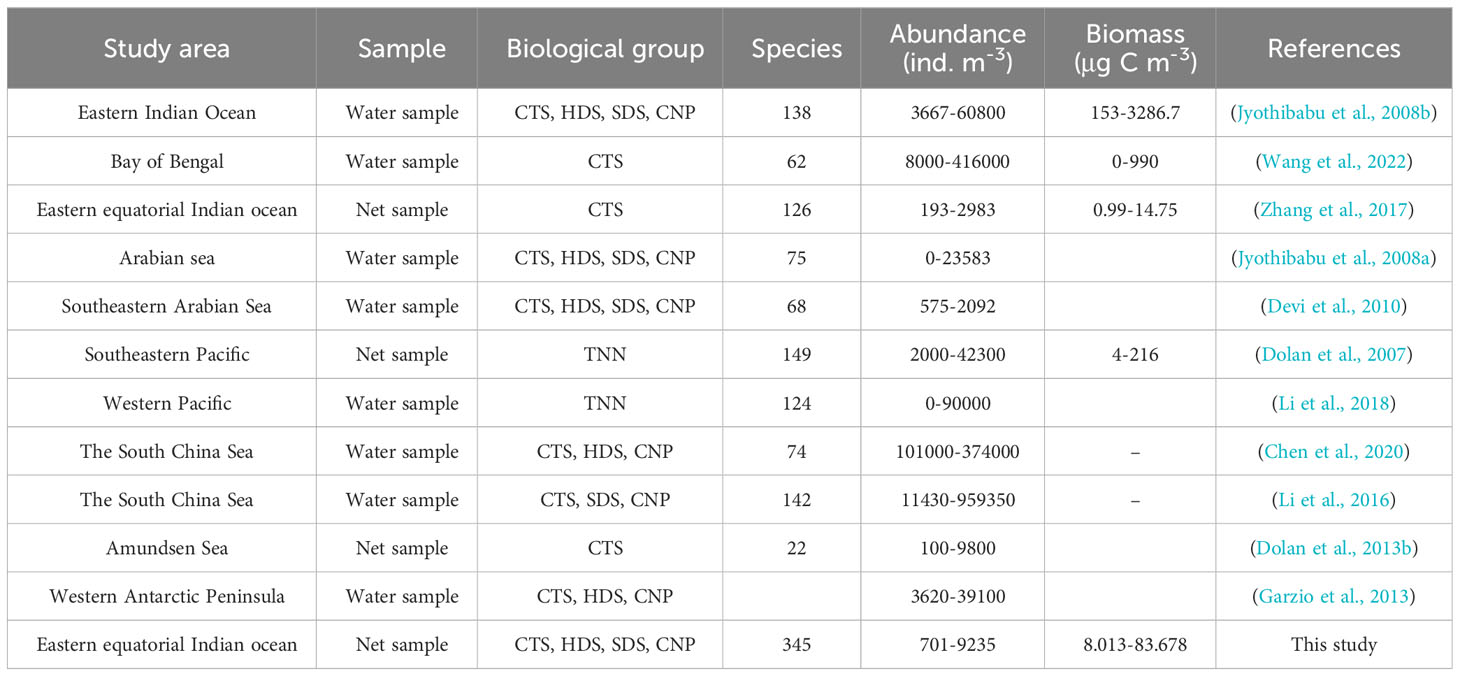
Table 4 Comparison of historical data on microzooplankton community structure in typical marine areas worldwide.
In the correlation analysis of nutrients and MZP biological variables, it can be seen that the concentration of DIP, DSi, and DIN showed a weak correlation with the biological variables of MZP, and they are generally positive. Among them, the abundances of P. perpusilla and G. polygramma showed significant positive correlation with DSi concentration at 0.05 and 0.001 confidence level. These results indicate that the abundance of MZP in the eastern equatorial Indian Ocean may be affected by the nutrient concentration levels of DSi, and different species may be affected by different dominant factors. This analysis is also supported by experiments in which nutrients affect the feeding of MZP (Calbet and Saiz, 2018). At the same time, we analyzed the correlation strength of the top 9 dominant species (Figure 10) and found that the abundance of A. armilla (Figure 5E) was relatively strongly correlated with various environmental factors. A. armilla is a kind of tintinnid with a lorica length of individual cells of about 25-33 μm (Supplementary Material Table 1), and the smaller the individual cell, the less tolerant it may be to environmental changes. This may be one of the reasons why CTS are often considered to serve as environmental indicator species (Jyothibabu et al., 2008a; Li et al., 2021; Wang et al., 2022). Therefore, this result may indicate that this species has a strong sensitivity to climate and current changes during the spring intermonsoon in the eastern Indian Ocean and may significantly change the population abundance with changes in external environmental factors. This may imply that A. armilla is a potential indicator of hydrologic changes in low-latitude oligotrophic oceans. However, we still need more detailed survey results and further analysis.
By comparing the historical research data in recent years (Table 4), we found relatively few studies on the whole group of MZP in the large area of the eastern equatorial Indian Ocean. They are mainly concentrated in the Arabian Sea and the western coastal area of the eastern Indian Ocean, while the investigation of the large area of the ocean current near the equator is still lacking, and some of the research is only for a specific group of studies. The results of this study of MZP in a large area of the eastern Indian Ocean are within the range of the known group in the tropical ocean (Jyothibabu et al., 2008b; Li et al., 2017; Zhang et al., 2017; Devi et al., 2020). However, the abundance and carbon biomass levels of each group of MZP in this survey were at a low level, while the survey results of species diversity were generally at a high level. We believe that the reason for this phenomenon may be due to the different methods of sample collection and the study of biological groups. Using a plankton net with 20 μm mesh sampling may lead to missing the organisms of MZP groups below 20 μm. However, the use of a plankton net to collect samples is helpful to increase the probability of studying most of the biological groups of MZP, to minimize the lack of data on the overall diversity of MZP, and to better understand the complete species diversity and community structure of MZP. In addition, the species composition of MZP in different sea areas also differs greatly. The diversity of MZP in tropical sea areas is higher, while the diversity of MZP in low-temperature sea waters at high latitudes is relatively low. Therefore, temperature may have an important impact on the species composition distribution of the MZP community. Our study area is a key location for the emergence of periodic ocean currents in the eastern Indian Ocean, and the emergence of intermonsoon Wyrtki jets may be one of the reasons for the difference from other studies. In summary, the survey of MZP in large areas of the eastern Indian Ocean still requires more data of similar standards to fully understand the level of MZP species diversity in the area.
By observing the species composition of MZP and comparing the levels of biotic variables and distribution patterns of different groups, we have gained a better understanding of the diversity and community structure of MZP in a tropical oligotrophic marine ecosystem. The species composition of the MZP community is controlled by protozoa. Among HDS and CTS as the dominant biological groups, the observations were consistent with those of Stoecker et al. (2014b) and Devi et al. (2010). CTS are more numerous at the genus level, while HDS are more numerous at the species level. That could mean CTS show greater variation in individual changes than HDS at the genus level, while HDS show greater variation in species changes than CTS at the species level. Their different trait may be to better adapt to environmental changes, so HDS may respond sensitively during periods of the monsoon reversal. The hyaline tintinnid tends to dominate the oceanic waters, and the agglutinated tintinnid is more prevalent in coastal waters. This may be due to the fact that coastal waters tend to have the phenomenon of phytoplankton flourishing, which leads to the existence of a large number of phytoplankton detritus from biological sources, and the input of surface runoff or atmospheric sedimentation brings a large number of abiotic mineral particles, all of which are conducive to the formation of the shell of the agglutinated tintinnid. For CNP, their traits are not very prominent in the immature stage, which may bring some limitations to species identification (Devi et al., 2020). SDS may be mainly benthic types, and as a result, studies about planktic groups living in seawater may not be adequate (Dolan et al., 2021). The abundance of CTS is greater than that of HDS, which might be explained by the greater retention of tintinnids (or their lorica) than HDS in seawater samples. CNP also accounted for a significant proportion of the abundance in each sample. This may be due to copepods often being the most abundant zooplankton in seawater throughout the world. Therefore, copepod larvae also have a high abundance level making them effective filter predators of phytoplankton with small algal cells (Li et al., 2017). In previous studies, there was a lack of research on the carbon biomass contribution of each group (Table 4). Our results indicate that HDS and CNP contribute to most of the carbon biomass of MZP in the eastern equatorial Indian Ocean, while CTS contributes relatively little carbon biomass. That may be due to the amount of carbon that CTS protoplasts can assimilate and conserve being more limited than that of other organisms such as cells of HDS and individuals of CNP. In addition, the selection of biovolume models and conversion factors may also influence the carbon biomass of MZP.
Generally, we believe that the diversity of a biological community is closely related to the stability of ecosystems. Among species relationships, the more complex and diverse a community is, the more stable the ecosystem tends to be. The biodiversity index is an important tool for analyzing the community structure, which helps us to describe the diversity of biotic populations from different focuses and compare the stability of different communities (Sun and Liu, 2004). Our experimental results showed large differences in the biodiversity indices of different taxa between stations I110 and I112. This may be because the habitat conditions of station I110 can support the survival of more MZP, especially for HDS. In fact, station I112 and station I110 are very similar in terms of hydrological and geographical distribution conditions, but they had completely different results. Therefore, we speculate that the spatial heterogeneity of the living environment may not be the main cause but is more likely to be caused by other disturbances and biological factors. The range of variation in evenness in our investigation is small (Table 3). This indicates that the individual number of each species occupies a similar proportion in the eastern Indian Ocean MZP community and its major groups, but there is no particularly prominent dominant species that can play a dominant role in the community, which may indicate that the ecological amplitude of MZP in the equatorial eastern Indian Ocean is relatively wide, so they do not need to live in a concentrated habitat. However, compared with HDS, the evenness variation of CTS groups was greater (Figures 8I, F). This may indicate that CTS is less tolerant to environmental changes than HDS; in other words, CTS is more sensitive to environmental changes than HDS. This may be one reason why CTS can be used as an indicator of environmental change (Pierce and Turner, 1992). In general, the biodiversity index of MZP and their major groups in the eastern Indian Ocean is at a high level, which indicates that the MZP community in the sea area is highly diverse, and the community structure may be in a relatively perfect and stable state. When analyzing the abundance and carbon biomass distribution (Figure 4) of various species in the community, especially the ecological types of dominant species (Figure 7), we found that the species with high abundance of MZP in the eastern equatorial Indian Ocean were mostly the eurytopic organisms. This demonstrates the MZP community in the eastern Indian Ocean may have strong community potential restoration. When the environment is damaged and then improved again, MZP communities can quickly return to their original levels in a relatively short period of time.
Combined with geographical analysis, it was found that group 4 is mainly distributed near the equator and may be strongly affected by Wyrtki jets during the spring intermonsoon (Figure 9). By analyzing the species composition of the top 5 in abundance ratio in these stations, it was found that A. armilla and C. teres had the largest proportion of repeats. The results of this analysis indicate that species such as A. armilla and C. teres are more dominant in MZP communities affected by Wyrtki jets. This species combination may play a positive role in explaining the function of the Wyrtki jets in dispersing and maintaining MZP populations in the eastern equatorial Indian Ocean during the spring intermonsoon period. However, the specific mechanism of the ocean current of influence on MZP remains to be further studied and discussed. Although the geographical distribution of these stations was not completely concentrated and uniform, most of the stations were consistent with the actual geographical locations, especially those stations that were affected by special ocean currents. This reflects the strong coupling effect between the MZP community and its external environment (Xue et al., 2016). Therefore, this kind of deviation should be understood and accepted because, under natural conditions, there is almost no uniform habitat, and the distribution of organisms in nature is not completely uniform and continuous.
Through this investigation, we studied the diversity and the relationship of major environmental factors to the change in the MZP community structure in the low-latitude oligotrophic eastern equatorial Indian Ocean during the spring intermonsoon. We identified a total of 63 genera and 340 species of MZP. The species diversity and abundance of the MZP community is dominated by HDS and CTS. The high species richness may indicate that the MZP community structure is relatively stable and could rapid recovery from environmental change. In contrast, the species diversity of HDS is higher and the abundance of CTS too, which may be due to the existence of a protective lorica of tintinnids, which makes it remain in seawater and more visible. However, CNP and HDS contribute more to the existing organic carbon stock, while the contribution of CTS to carbon biomass is small. Periodic currents such as Wyrtki jets in the eastern equatorial Indian Ocean during the spring intermonsoon strongly affect the hydrological characteristics of the 200 m depth seawaters of the eastern Indian Ocean, thus changing the abundance level and distribution pattern of MZP in the sea area. The environmental factors such as temperature, salinity, and integrated chlorophyll a were weakly correlated with the biological variables of MZP, negatively correlated with temperature, and positively correlated with salinity in general. In the spatial distribution pattern, there was a good similarity between MZP biological variables and environmental variables, in which temperature may be the dominant factor affecting the distribution of MZP. In the equatorial oligotrophic ocean, low temperatures can obviously limit the expansion of the MZP community. Most of the dominant species of the MZP community in the eastern equatorial Indian Ocean are cosmopolitan. The CNP may be the eurytopic group, the most dominant species in the group of CTS is Eutintinnus tenuis, and the most dominant species in the group of HDS is Ceratium teres. However, CTS may be more sensitive to environmental changes than HDS, and Ascampbelliella armilla may be a potential indicator species responding to the Wyrtki jet in the equatorial eastern Indian Ocean. In addition, DSi can influence the abundance or distribution pattern of the dominant species of MZP. In this article, we propose that more detailed experimental methods should be established to estimate the carbon biomass of MZP, which can reflect the actual situation of organisms, so as to provide a basis for further revealing the ecological functions of MZP in the microbial food web. In addition, detailed experiments or investigations are still needed to analyze the relationship between size-fractionated phytoplankton and MZP community changes, which has important significance in supporting the selective feeding behavior of MZP. Further study on the ecological types and indicator species of tintinnids in this sea area may help to reveal the interaction mechanism between the environment and organisms in this sea area.
The original contributions presented in the study are included in the article/Supplementary Materials, further inquiries can be directed to the corresponding author/s.
The manuscript presents research on animals that do not require ethical approval for their study.
JS: Conceptualization, Methodology, Project administration, Resources, Supervision, Visualization, and Review and editing. JZ: Sample identification, counting, and measurement, Data analysis, Writing the manuscript, and Visualization. All authors contributed to the article and approved the submitted version.
This research was financially supported by the National Nature Science Foundation of China grants (41876134, 41676112, and 41276124), the State Key Laboratory of Biogeology and Environmental Geology, China University of Geosciences (No. GKZ22Y656), and the Changjiang Scholar Program of Chinese Ministry of Education (T2014253) awarded to JS. JS also acknowledges support by Projects of Southern Marine Science and Engineering Guangdong Laboratory (Zhuhai) (SML2021SP204, SML2022005).
We would like to thank the Open Cruise Project in Eastern Indian Ocean of National Nature Science Foundation of China (Nos: 41276124) for sharing their research voyage (NORC2016-10). We are extremely grateful to the research team from the South China Sea Institute of Oceanology Chinese Academy of Sciences for providing the sea area temperature and salinity data. We thank the crew of the R/V “SHIYAN 1” for their help with the cruise operation. We also thank Xingzhou Wang and Guicheng Zhang for their valuable help.
The authors declare that the research was conducted in the absence of any commercial or financial relationships that could be construed as a potential conflict of interest.
All claims expressed in this article are solely those of the authors and do not necessarily represent those of their affiliated organizations, or those of the publisher, the editors and the reviewers. Any product that may be evaluated in this article, or claim that may be made by its manufacturer, is not guaranteed or endorsed by the publisher.
The Supplementary Material for this article can be found online at: https://www.frontiersin.org/articles/10.3389/fmars.2023.1249281/full#supplementary-material
Abrams P. A. (1989). Perspectives in ecological theory. Trends Ecol. Evol. 4, 220–221. doi: 10.1016/0169-5347(89)90082-7
Al-Yamani F., Madhusoodhanan R., Skryabin V., Al -Said T. (2019). The response of microzooplankton (tintinnid) community to salinity related environmental changes in a hypersaline marine system in the northwestern Arabian Gulf. Deep-Sea Res. Part Ii-Topical Stud. Oceanogr 166, 151–170. doi: 10.1016/j.dsr2.2019.02.005
Azam F., Fenchel T., Field J., Thingstad T. (1983). The ecological role of water-column microbes in the sea. Mar. Ecol. Prog. Series 10, 257–263. doi: 10.3354/meps010257
Beers J. R., Stewart G. L. (1969). Micro-zooplankton and its abundance relative to the larger zooplankton and other seston components. Mar. Biol. 4, 182–189. doi: 10.1007/BF00393891
Biswas H., Gadi S. D., Ramana V. V., Bharathi M. D., Priyan R. K., Manjari D. T., et al. (2012). Enhanced abundance of tintinnids under elevated CO2 level from coastal Bay of Bengal. BIODIVERSITY AND Conserv. 21, 1309–1326. doi: 10.1007/s10531-011-0209-7
Broglio E., Saiz E., Calbet A., Trepat I., Alcaraz M. (2004). Trophic impact and prey selection by crustacean zooplankton on the microbial communities of an oligotrophic coastal area (NW Mediterranean Sea). Aquat. Microbial Ecol. 35, 65–78. doi: 10.3354/ame035065
Calbet A. (2008). The trophic roles of microzooplankton in marine systems. Ices J. Mar. Sci. 65, 325–331. doi: 10.1093/icesjms/fsn013
Calbet A., Landry M. R. (1999). Mesozooplankton influences on the microbial food web: Direct and indirect trophic interactions in the oligotrophic open ocean. Limnology Oceanogr 44, 1370–1380. doi: 10.4319/lo.1999.44.6.1370
Calbet A., Landry M. R. (2004). Phytoplankton growth, microzooplankton grazing, and carbon cycling in marine systems. Limnology Oceanogr 49, 51–57. doi: 10.4319/lo.2004.49.1.0051
Calbet A., Saiz E. (2005). The ciliate-copepod link in marine ecosystems. Aquat. Microbial Ecol. 38, 157–167. doi: 10.3354/ame038157
Calbet A., Saiz E. (2018). How much is enough for nutrients in microzooplankton dilution grazing experiments? J. Plankton Res. 40, 109–117. doi: 10.1093/plankt/fbx070
Caron D. A., Hutchins D. A. (2012). The effects of changing climate on microzooplankton grazing and community structure: drivers, predictions and knowledge gaps. J. Plankton Res. 35, 235–252. doi: 10.1093/plankt/fbs091
Caron D. A., Michaels A. F., Swanberg N. R., Howse F. A. (1995). Primary productivity by symbiont-bearing planktonic sarcodines (Acantharia, Radiolaria, Foraminifera) in surface waters near Bermuda. J. Plankton Res. 17, 103–129. doi: 10.1093/plankt/17.1.103
Chen D. (2019). The study of microzooplankton grazing in the eastern Indian Ocean and South China sea (Tian Jin: Tianjin University of Science & Technology).
Chen D., Guo C., Yu L., Lu Y., Sun J. (2020). Phytoplankton growth and microzooplankton grazing in the central and northern South China Sea in the spring intermonsoon season of 2017. Acta Oceanologica Sin. 39, 84–95. doi: 10.1007/s13131-020-1593-1
Devi C. R. A., Jyothibabu R., Sabu P., Jacob J., Habeebrehman H., Prabhakaran M. P., et al. (2010). Seasonal variations and trophic ecology of microzooplankton in the southeastern Arabian Sea. Continental Shelf Res. 30, 1070–1084. doi: 10.1016/j.csr.2010.02.007
Devi C. R. A., Sabu P., Naik R. K., Bhaskar P. V., Achuthankutty C. T., Soares M., et al. (2020). Microzooplankton and the plankton food web in the subtropical frontal region of the Indian Ocean sector of the Southern Ocean during austral summer 2012. Deep Sea Res. Part II: Topical Stud. Oceanogr 178, 104849. doi: 10.1016/j.dsr2.2020.104849
Dolan J. R., Montagnes D., Agatha S., Coats W., Stoecker D. K. (2013a). The biology and ecology of tintinnid ciliates: models for marine plankton (Oxford: Wiley-Blackwell).
Dolan J. R., Moon J. K., Yang E. J. (2021). Notes on the Occurrence of Tintinnid Ciliates, and the Nasselarian Radiolarian Amphimelissa setosa of the Marine Microzooplankton, in the Chukchi Sea (Arctic Ocean) Sampled each August from 2011 to 2020. Acta Protozoologica 60, 1–11. doi: 10.4467/16890027AP.21.001.14061
Dolan J. R., Ritchie M. E., Ras J. (2007). The "neutral" community structure of planktonic herbivores, tintinnid ciliates of the microzooplankton, across the SE Tropical Pacific Ocean. Biogeosciences 4, 297–310. doi: 10.5194/bg-4-297-2007
Dolan J. R., Son W., La H. S., Park J., Yang E. J. (2022b). Tintinnid ciliates (marine microzooplankton) of the Ross Sea. Polar Res. 41, 82–83. doi: 10.33265/polar.v41.8382
Dolan J. R., Yang E. J., Lee S. H., Kim S. Y. (2013b). Tintinnid ciliates of Amundsen Sea (Antarctica) plankton communities. Polar Res. 32, 12. doi: 10.3402/polar.v32i0.19784
Evelyn B. S., Barry F. S. (2007). Heterotrophic dinoilagellates: a significant component of microzooplankton biomass and major grazers of diatoms in the sea. Mar. Ecol. Prog. Ser. 352, 187–197. doi: 10.3354/meps07161
Garzio L. M., Steinberg D. K., Erickson M., Ducklow H. W. (2013). Microzooplankton grazing along the Western Antarctic Peninsula. Aquat. Microbial Ecol. 70, 215–232. doi: 10.3354/ame01655
Gilron G. L., Lynn D. H. (1989). Assuming a 50% cell occupancy of the lorica overestimates tintinnine ciliate biomass. Mar. Biol. 103, 413–416. doi: 10.1007/BF00397276
Gomez F. (2007). Trends on the distribution of ciliates in the open Pacific Ocean. Acta Oecologica-International J. Ecol. 32, 188–202. doi: 10.1016/j.actao.2007.04.002
Hada Y. (1970). The protozoan plankton of the Antarctic and Subantarctic seas. JARE Sci. Rep. Ser. E Biol. 31, 1–51.
Hamilton E. I. (1984). A manual of chemical & biological methods for seawater analysis. Mar. pollut. Bull. 15, 419–420. doi: 10.1016/0025-326X(84)90262-5
Hillebrand H., Dürselen C.-D., Kirschtel D., Pollingher U., Zohary T. (1999). Biovolume calculation for pelagic and benthic microalgae. J. Phycology 35, 403–424. doi: 10.1046/j.1529-8817.1999.3520403.x
Isshiki K., Sohrin Y., Nakayama E. (1991). Form of dissolved silicon in seawater. Mar. Chem. 32, 1–8. doi: 10.1016/0304-4203(91)90021-N
Jyothibabu R., Devi C. R. A., Madhu N. V., Sabu P., Jayalakshmy K. V., Jacob J., et al. (2008a). The response of microzooplankton (20-200 μm) to coastal upwelling and summer stratification in the southeastern Arabian Sea. Continental Shelf Res. 28, 653–671. doi: 10.1016/j.csr.2007.12.001
Jyothibabu R., Madhu N. V., Maheswaran P. A., Jayalakshmy K. V., Nair K. K. C., Achuthankutty C. T. (2008b). Seasonal variation of microzooplankton (20-200 um) and its possible implications on the vertical carbon flux in the western Bay of Bengal. Continental Shelf Res. 28, 737–755. doi: 10.1016/j.csr.2007.12.011
Kofoid C. A., Campbell A. S. (1929). A conspectus of the marine and freshwater Ciliata belonging to the suborder Tintinnoinea, with descriptions of new species, principally from the Agassiz Expedition to the eastern tropical Pacific 1904-1905 (Berkeley, CA: University of California Publications in Zoology 34).
Kofoid C. A., Campbell A. S. (1939). “Reports on the scientific results of the expedition to the eastern tropical Pacific, in charge of Alexander Agassiz, by U.S. Fish Commission Steamer Albatross from October 1904 to March 1905,” in The Ciliata: The Tintinnoinea (Bulletin of the Museum of Comparative Zoology of Harvard College, vol. VII. (California: Cambridge University, Harvard (Lieut.-Commander LM Garrett, USN commanding).
Kumar S. P., Muraleedharan P. M., Prasad T. G., Gauns M., Ramaiah N., De Souza S. N., et al. (2002). Why is the Bay of Bengal less productive during summer monsoon compared to the Arabian Sea? Geophys Res. Lett. 29, 4. doi: 10.1029/2002GL016013
Landry M. R., Hassett R. P. (1982). Estimating the grazing impact of marine micro-zooplankton. Mar. Biol. 67, 283–288. doi: 10.1007/BF00397668
Lessard E. J., Swift E. (1985). Species-specific grazing rates of heterotrophic dinoflagellates in oceanic waters, measured with a dual-label radioisotope technique. Mar. Biol. 87, 289–296. doi: 10.1007/BF00397808
Li Z., Sun J., Liu H., Bing X., Zhang C., Rui Z. (2016). Microzooplankton communities in the northern south China sea in summer. Haiyang Xuebao 38, 31–42. doi: 10.3969/j.issn.0253-4193.2016.04.003
Li H. B., Xuan J., Wang C. F., Chen Z. H., Gregori G., Zhao Y., et al. (2021). Summertime tintinnid community in the surface waters across the north pacific transition zone. Front. Microbiol. 12, 16. doi: 10.3389/fmicb.2021.697801
Li K., Yin J., Tan Y., Huang L., Li G. (2017). Diversity and abundance of epipelagic larvaceans and calanoid copepods in the eastern equatorial Indian Ocean during the spring inter-monsoon. Indian J. Geo-Marine Sci. 46, 1371–1380. http://nopr.niscpr.res.in/handle/123456789/42242.
Li H. B., Zhang W. C., Zhao Y., Zhao L., Dong Y., Wang C. F., et al. (2018). Tintinnid diversity in the tropical West Pacific Ocean. Acta Oceanologica Sin. 37, 218–228. doi: 10.1007/s13131-018-1148-x
Lin X., Qi Y., Cheng X. (2014). Hydrographical features in the Eastern Indian Ocean during March–May. J. Trop. oceanogr 33, 1–9. doi: 10.3969/j.issn.1009-5470.2014.03.001
Liu H. B., Suzuki K., Saino T. (2002). Phytoplankton growth, and microzooplankton grazing in the subarctic Pacific Ocean and the Bering Sea during summer 1999. Deep-Sea Res. Part I-Oceanographic Res. Papers 49, 363–375. doi: 10.1016/S0967-0637(01)00056-5
MacArthur R. (1955). Fluctuations of animal populations and a measure of community stability. Ecology 36, 533–536. doi: 10.2307/1929601
Menden-Deuer S., Lessard E. J. (2000). Carbon to volume relationships for dinoflagellates, diatoms, and other protist plankton. Limnology Oceanogr 45, 569–579. doi: 10.4319/lo.2000.45.3.0569
Nagura M., Mcphaden M. J. (2018). The shallow overturning circulation in the Indian ocean. J. Phys. Oceanogr 48, 413–434. doi: 10.1175/JPO-D-17-0127.1
Pai S. C., Tsau Y. J., Yang T. I. (2001). pH and buffering capacity problems involved in the determination of ammonia in saline water using the indophenol blue spectrophotometric method. Analytica Chimica Acta 434, 209–216. doi: 10.1016/S0003-2670(01)00851-0
Paterson H. L., Knott B., Waite A. M. (2007). Microzooplankton community structure and grazing on phytoplankton, in an eddy pair in the Indian Ocean off Western Australia. Deep Sea Res. Part II: Topical Stud. Oceanogr 54, 1076–1093. doi:10.1016/j.dsr2.2006.12.011
Patey M. D., Rijkenberg M. J. A., Statham P. J., Stinchcombe M. C., Achterberg E. P., Mowlem M. (2008). Determination of nitrate and phosphate in seawater at nanomolar concentrations. Trac-Trends Analytical Chem. 27, 169–182. doi: 10.1016/j.trac.2007.12.006
Peng S., Qian Y., Lumpkin R., Du Y., Wang D., Li P. (2015). Characteristics of the near-surface currents in the Indian ocean as deduced from satellite-tracked surface drifters. Part I: pseudo-eulerian statistics. J. Phys. Oceanogr 45, 441–458. doi: 10.1175/JPO-D-14-0050.1
Pielou E. C. J. (1966). The measurement of diversity in different types of biological collections. J. Theor. Biol. 13, 131–144. doi: 10.1016/0022-5193(66)90013-0
Pierce R., Turner J. (1992). Ecology of plankton ciliates in marine food webs. Rev. Aquat. Sci. 6, 139–181.
Pomeroy L. R. (1974). The ocean's food web, A changing paradigm. BioScience 24, 499–504. doi: 10.2307/1296885
Putt M., Stoecker D. K. (1989). An experimentally determined carbon : volume ratio for marine \"oligotrichous\" ciliates from estuarine and coastal waters. Limnology Oceanogr 34, 1097–1103. doi: 10.4319/lo.1989.34.6.1097
Ramaiah N., Raghukumar S., Mangesh G., Madhupratap M. (2005). Seasonal variations in carbon biomass of bacteria, thraustochytrids and microzooplankton in the Northern Arabian Sea. Deep Sea Res. Part II: Topical Stud. Oceanogr 52, 1910–1921. doi: 10.1016/j.dsr2.2005.05.004
Rychert K. (2011). Dependence between volumes of protoplast and lorica in lugol-fixed tintinnid ciliates. Protist 162, 249–252. doi: 10.1016/j.protis.2010.05.004
Schott F. A., Xie S. P., Mccreary J. P. (2009). Indian Ocean CirculstIion and climate variability. Rev. Geophysics 47, 46. doi: 10.1029/2007RG000245
Shannon C. E. (1950). The mathematical theory of communication. Bell Labs Tech. J. 3, 31–32. doi: 10.1063/1.3067010
Shetye S. R., Shenoi S. S. C., Gouveia A. D., Michael G. S., Sundar D., Nampoothiri G. (1991). Wind-driven coastal upwelling along the western boundary of the Bay of Bengal during the southwest monsoon. Continental Shelf Res. 11, 1397–1408. doi: 10.1016/0278-4343(91)90042-5
Sieburth J. M., Smetacek V., Lenz J. (1978). Pelagic ecosystem structure: Heterotrophic compartments of the plankton and their relationship to plankton size fractions 1. Limnology Oceanogr 23, 1256–1263. doi: 10.4319/lo.1978.23.6.1256
Steinberg D. K., Landry M. R., Annual R. (2017). Zooplankton and the ocean carbon cycle. Annu. Rev. OF Mar. Sci. 9, 413–444. doi: 10.1146/annurev-marine-010814-015924
Stoecker D. K., Weigel A., Goes J. I. (2014a). Microzooplankton grazing in the Eastern Bering Sea in summer. Deep Sea Res. Part II: Topical Stud. Oceanogr 109, 145–156. doi: 10.1016/j.dsr2.2013.09.017
Stoecker D. K., Weigel A. C., Stockwell D. A., Lomas M. W. (2014b). Microzooplankton: Abundance, biomass and contribution to chlorophyll in the Eastern Bering Sea in summer. Deep-Sea Res. Part Ii-Topical Stud. Oceanogr 109, 134–144. doi: 10.1016/j.dsr2.2013.09.007
Strutton P. G., Coles V. J., Hood R. R., Matear R. J., Mcphaden M. J., Phillips H. E. (2015). Biogeochemical variability in the central equatorial Indian Ocean during the monsoon transition. Biogeosciences 12, 2367–2382. doi: 10.5194/bg-12-2367-2015
Sun J. (2011). Marine phytoplankton and biological carbon sink. Acta Ecologica Sin. 31, 7. doi: CNKI:SUN:STXB.0.2011-18-031
Sun J., Guo S. ,. J. (2011). Dinoflagellate heterotrophy. Acta Ecologica Sin. 31, 6270–6286. doi: CNKI:SUN:STXB.0.2011-20-048
Sun J., Liu D. (2002). The Preliminary notion on nomenclature of common phytoplankton in China seas waters. Oceanologia Et Limnologia Sin. 33, 271–286. doi: 10.1088/1009-1963/11/5/313
Sun J., Liu D. (2003). Geometric models for calculating cell biovolume and surface area for phytoplankton. J. Plankton Res. 25, 1331–1346. doi: 10.1093/plankt/fbg096
Sun J., Liu D. (2004). The application of diversity indices in marine phytoplankton studies. Haiyang Xuebao 26, 62. doi: 10.3321/j.issn:0253-4193.2004.01.007
Sun J., Song S. Q., Wang D., Xu Z. L. (2007). Estimating Calanus sinicus grazing on phytoplankton and microzooplankton. Acta EcoloGgica Sinca 27, 14. doi: 10.3969/j.issn.1673-5102.2003.02.007
Uitz J., Claustre H., Morel A., Hooker S. B. (2006). Vertical distribution of phytoplankton communities in open ocean: An assessment based on surface chlorophyll. J. Geophys Research-Oceans 111, 23. doi: 10.1029/2005JC003207
Uye S.-I., Nagano N., Tamaki H. (1996). Geographical and seasonal variations in abundance, biomass and estimated production rates of microzooplankton in the Inland Sea of Japan. J. Oceanogr 52, 689–703. doi: 10.1007/BF02239460
Verity P. G., Lagdon C. (1984). Relationships between lorica volume, carbon, nitrogen, and ATP content of tintinnids In Narragansett Bay. J. Plankton Res. 6, 859–868. doi: 10.1093/plankt/6.5.859
Wang C., Li H., Zhang W., Zhao L., Zhao Y., Xiao T. (2016). Analyzing the tintinnid community structure and distribution in the surface waters southeast of Hawaii from a cruise in 2013. Biodiversity Sci. 24, 831–837. doi: 10.17520/biods.2016030
Wang C., Zhao Y., Du P., Ma X., Li S., Li H., et al. (2022). Planktonic ciliate community structure and its distribution in the oxygen minimum zones in the Bay of Bengal (eastern Indian Ocean). J. Sea Res. 190, 15. doi: 10.1016/j.seares.2022.102311
Wiggert J. D., Murtugudde R. G., Christian J. R. (2006). Annual ecosystem variability in the tropical Indian Ocean: Results of a coupled bio-physical ocean general circulation model. Deep-Sea Res. Part Ii-Topical Stud. Oceanogr 53, 644–676. doi: 10.1016/j.dsr2.2006.01.027
Wishner K. F., Seibel B., Outram D. (2020). Ocean deoxygenation and copepods: coping with oxygen minimum zone variability. Biogeosciences 17, 2315–2339. doi: 10.5194/bg-17-2315-2020
Wyrtki K. (1973). An equatorial jet in the Indian ocean. Science 181, 262–264. doi: 10.1126/science.181.4096.262
Xu Z. L., Chen Y. Q. (1989). Aggregated intensity of dominant species of zooplankton in autumn in the East China Sea and Yellow Sea. J. Ecol. 8, 13–15. doi: 10.13292/j.1000-4890.1989.0055
Xue B., Sun J., Li T. (2016). Phytoplankton community structure of northern South China Sea in summer of 2014. Acta Oceanologica Sin. 38, 56–65. doi: 10.3969/j.issn.0253-4193.2016.04.005
Yang E. J., Choi J. K., Hyun J. H. (2008). Seasonal variation in the community and size structure of nano- and microzooplankton in Gyeonggi Bay, Yellow Sea. Estuar. Coast. Shelf Sci. 77, 320–330. doi: 10.1016/j.ecss.2007.09.034
Yong Y. L., Lee C. W., Bong C. W., Chew L., Chong V. C. (2022). The role of microzooplankton grazing in the microbial food web of a tropical mangrove estuary. Estuar. Coast. Shelf Sci. 275, 13. doi: 10.1016/j.ecss.2022.107969
Zhang W., Feng M., Yu Y., Zhang C., Xiao T. (2012). An Illustrated Guide to Contemporary Tintinnids in the World (Beijing: Science Press).
Zhang C., Sun J., Wang D., Song S., Zhang X., Munir S. (2017). Tintinnid community structure in the eastern equatorial Indian Ocean during the spring inter-monsoon period. Aquat. Biol. 26, 87–100. doi: 10.3354/ab00677
Zhang W., Wang R. (2000). Microzooplankton and their grazing pressure of phytoplankton in Bohai sea. Oceanologia Et Limnologia Sin. 31, 252–257. doi: 10.11693/hyhz200003004004
Keywords: microzooplankton, eastern Indian Ocean, hydrological environment, diversity, horizontal distribution, dominant species, carbon biomass
Citation: Zhai J and Sun J (2023) Diversity and community structure of microzooplankton in the eastern Indian Ocean during the inter-monsoon period. Front. Mar. Sci. 10:1249281. doi: 10.3389/fmars.2023.1249281
Received: 28 June 2023; Accepted: 23 October 2023;
Published: 15 November 2023.
Edited by:
Michael Rappe, University of Hawaii at Manoa, United StatesReviewed by:
Vankara Venkataramana, National Centre for Polar and Ocean Research (NCPOR), IndiaCopyright © 2023 Zhai and Sun. This is an open-access article distributed under the terms of the Creative Commons Attribution License (CC BY). The use, distribution or reproduction in other forums is permitted, provided the original author(s) and the copyright owner(s) are credited and that the original publication in this journal is cited, in accordance with accepted academic practice. No use, distribution or reproduction is permitted which does not comply with these terms.
*Correspondence: Jun Sun, cGh5dG9wbGFua3RvbkAxNjMuY29t
Disclaimer: All claims expressed in this article are solely those of the authors and do not necessarily represent those of their affiliated organizations, or those of the publisher, the editors and the reviewers. Any product that may be evaluated in this article or claim that may be made by its manufacturer is not guaranteed or endorsed by the publisher.
Research integrity at Frontiers
Learn more about the work of our research integrity team to safeguard the quality of each article we publish.